Bioclimatic inference based on mammal community using machine learning regression models: perspectives for paleoecological studies

1 Introduction

Paleoclimate studies allow quantitative inferences of the magnitudes, rates, and mechanisms of climate change and provide direct evidence on biodiversity responses to past environmental changes (Bertrand et al., 2011; Cerling et al., 2011; Lorenzen et al., 2011; Lyons et al., 2016; Clavel and Morlon, 2017; Nogués-Bravo et al., 2018; Mondanaro et al., 2021; Timmermann et al., 2022). Currently, a wide variety of climate proxy data can be gathered to infer past climatic conditions at various temporal and spatial coverage. Some of the most widely employed proxy data include tree rings, corals, ice cores, sediments, plankton, and pollen (see, e.g., Jansen et al., 2007; Jones et al., 2009; Birks et al., 2010; Bartlein et al., 2011; Krapp et al., 2021; Andrews et al., 2022). However, many key archeological and paleontological deposits do not preserve such sources of evidence. Where available, fossil faunas can alternatively be used to help decipher more spatiotemporally constrained environmental and climatic conditions, assuming that many taxa are indicative of ecosystem structure (Grayson, 1981; Andrews, 1995; Damuth and Janis, 2011; Lyman, 2017). Over the years, paleontologists and archeozoologists have developed a pool of new methods of paleoclimatic inference based on faunal fossil remains, especially those of mammals, with a distinction being drawn between taxonomic approaches (when fossils are identified to the highest taxonomic level, ideally the species) and taxon-free approaches (when analyses are independent of the taxonomy). Taxonomic approaches typically use distribution, ecological niche and habitat preference of modern related species, while taxon-free methods are based on functional morphology, species richness or community composition, for instance (for examples and syntheses, see Mendoza et al., 2005; Reed et al., 2013; Andrews and Hixson, 2014; Lyman, 2017). Opting for one method over another may result from several analytical and practical considerations such as the number of fossil specimens available for a fossil site, the spatial and temporal scale of the analysis, or the researcher’s expertise. However, the performance of a climatic reconstruction ultimately depends on the quality of the fossil record, which can be assessed using taphonomic analyses (e.g., identifiability of the remains, geochronology, taphonomic alterations).

More recently, advancements in multivariate statistical analysis have led to improved accuracy and spatio-temporal resolution in climatic inference methods based on faunal evidence, leveraging techniques such as linear discriminant analysis and transfer functions (in palaeoenvironmental research, a transfer function is a statistical function that models the relationship between paleobiotic data and climate or environmental parameters; see Sachs et al., 1977). Two common recent approaches are the Bioclimatic Analysis (Hernández Fernández, 2001; Hernández Fernández, 2006; Royer et al., 2020) and the Mutual Ecogeographic Range (Blain et al., 2009; Fagoaga et al., 2019), which can be used to predict categorical and/or numerical variables. Both methods are based on the geographical range of identified species and provide high accuracy for environmental interpretation. However, their application on fossil sites is not always straightforward: they were initially developed for fossil localities from across the Palearctic realm, which involved extensive collection of fauna data from modern localities within the same realm, and their applicability to other parts of the world thus require significant effort in additional data collection; they are not well suited to no-analog communities (i.e., those whose composition is unlike any found today); they require a high and homogeneous taxonomic resolution (ideally, all specimens should be identified to the species level). There are many fossil localities where such taxonomic determination is seldom achieved, such as pleistocene hominin-bearing deposits from southern and Eastern Africa (Avery, 2007). In these localities, faunal lists cannot achieve species resolution. In such a context, the application of the aforementioned paleoclimatic methods becomes challenging and does not guarantee high, consistent accuracy.

Over the past two decades, focus has been placed on advancing machine learning (ML) algorithms to effectively tackle predictions on increasingly larger datasets characterized by complex patterns and nonlinear interactions. ML techniques are now routinely used in environmental and ecological sciences for a wide range of complex tasks such as global weather forecasting (Dueben and Bauer, 2018; Gibson et al., 2021), air pollution estimation (Bellinger et al., 2017; Chen et al., 2019), wildfire management (Jain et al., 2020), or biodiversity assessment and monitoring (Knudby et al., 2010; Kwok, 2019; Tuia et al., 2021). However, there are two main challenges that often hamper the accuracy and applicability of ML methods to biological data: (1) the low number of observations available for constructing the dataset and (2) the difficulty of integrating various levels of taxonomic identifications. These two challenges are particularly prevalent with paleontological remains, due to the fragmentary nature of fossils and the chronological gaps between assemblages (Lyman, 2017).

In this study, we introduce a new ML approach for the automated prediction of various environmental and climatic variables based on the composition of the faunal community. This approach enables the generation of precise predictions using faunal lists with various taxonomic resolutions, irrespective of the geographic region, and without the requirement of a large dataset of modern faunal localities to ensure robust model performance. The objectives of this paper are to describe the methodology and evaluate its precision using modern fauna. We applied this approach to African rodent communities, as they have already been extensively used as proxy indicators for reconstructing Quaternary past environments (Andrews, 1990; Fernández-Jalvo et al., 1998; Avery, 2001; Avery, 2007; Matthews et al., 2011; Stoetzel et al., 2018; Matthews et al., 2020). We developed an integrative approach for constructing neo-ecological large-scale datasets and utilized a combination of seven linear and non-linear machine learning (ML) algorithms to achieve highly accurate predictions of climatic variables across various locations throughout Africa. We devised a specific geographical cross-validation in order to mitigate effects of spatial autocorrelation on the dependence of the data. We evaluated the performance of the algorithms to determine the most accurate ones for each variable, considering also their ease of implementation in our selection process, and validated the predictions using modern comparative reference data. This methodology can be easily adapted to other systems to meet specific requirements, for example, by including other biotic proxies (such as vegetation or other fauna) or by adjusting the geographical resolution (focusing on a specific area or covering the entire world). As this paper aims to present the new methodology, its application to fossil faunal lists is reserved for future research, which will provide an opportunity to further discuss issues specifically related to the fossil context. Our study showcases the versatility of ML techniques in reconstructing past and present environments, underscoring their promising potential for utilization in the fields of archaeology and paleontology.

2 Materials and methods

2.1 Data collection

We trained the algorithms to infer climatic variables based on the presence of taxa at a given locality. To achieve this, we constructed a large dataset comprising numerous localities (10x10 km grid covering the entire African continent) with associated bioclimatic conditions (using the Worldclim set of 19 bioclimatic variables), as well as the list of rodents present in each locality (Figure 1). In the sections below, we detail the procedure by which this dataset can be automatically built.

FIGURE 1

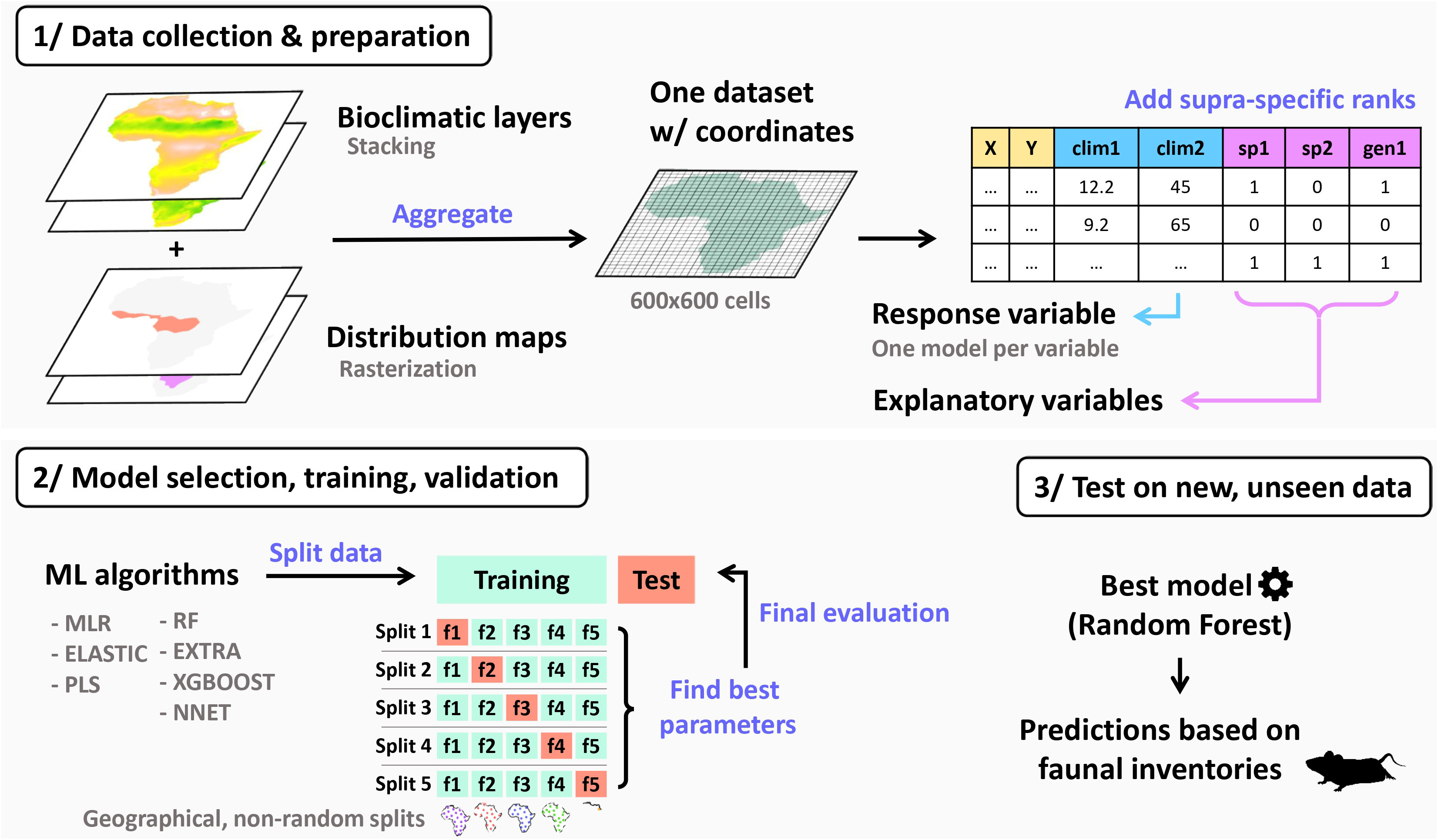
Figure 1 Data aggregation and machine learning (ML) workflow depicting the different analytical steps. The data used in this study were obtained by combining species distribution maps with bioclimatic layers into a single dataset. Explanatory variables, which include species and supra-specific occurrence information, are utilized to predict a single bioclimatic variable (response variable) through the application of various machine learning algorithms with a geographically-based cross validation procedure. Random forest algorithm achieved the highest predictive performance.

The efficacy of a ML method is dependent on the quality of the computation architecture and the availability of a large and appropriate amount of training data (Cui and Gong, 2018). The acquisition of data is therefore a crucial issue, yet ecologists rarely have access to an extended, quality annotated data set. This limitation can be a significant constraint in environmental studies, where the need for extrapolation is high (for instance, predicting changes in aridity) but the training and test data within the sought range of prediction are limited. Recent studies seeking to reconstruct past environmental conditions from fauna using statistical computing and ML methods (e.g. Žliobaitė, 2019; Spradley et al., 2019; Royer et al., 2020) have used limited datasets with a quantity of input data restricted by several factors, such as sampling effort or the availability of open and accessible published faunal lists. Occurrence data of fauna species typically come from sources such as the Global Biodiversity Information Facility (GBIF), published field surveys and park or game reserve lists (see, for instance, the Information Center for the Environment (ICE) Biological Inventories of the World’s Protected Areas), and primary literature. There are many factors that preclude the collection of species occurrence observations and thus affect the comprehensiveness and representativeness of these data (Rondinini et al., 2006), and the minimum sample size required for producing meaningful predictions is usually difficult to estimate. One way to address this problem while meeting data requirements is to combine gridded weather and climate data with range maps of modern African rodent species.

2.1.1 Bioclimatic data

Bioclimatic data was retrieved from Worldclim 2.1 (Fick and Hijmans, 2017) at a resolution of 5 minutes (10x10km). The Worldclim dataset consists of 19 spatial raster images representing average, minimum and maximum temperatures and precipitation (Table 1). Data were collected from various weather stations worldwide and represent averages for the years 1970–2000. An additional spatial map for evapotranspiration (ET, in mm/day) was obtained from the Consortium for Spatial Information (CGIAR-CSI) GeoPortal (https://cgiarcsi.community). In total, we used approximately 350,000 10x10 km cells with associated climatic measurements to ensure complete coverage throughout the African continent. This resolution offers a dataset that is large enough to obtain high accuracy and of sufficient resolution to capture the influence of habitat heterogeneity on the structure of African rodent communites.

TABLE 1

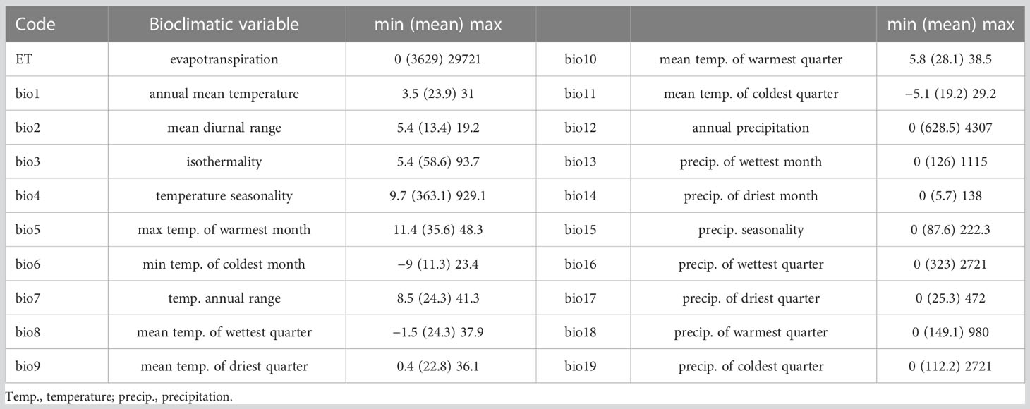
Table 1 The 20 bioclimatic variables used for the study.

In this study, we focused on modelling the 20 climatic variables independently, based on the presence or absence of rodent taxa. We chose to consider not only annual trends (e.g., mean annual temperature or precipitation) but also extreme or limiting environmental factors (e.g., temperature of the warmest month or precipitation of the wettest quarter) as relevant for reconstructing climate conditions. Integrating these “secondary” variables allows us to represent not only global climate conditions, but also seasonality components, which are essential to understand ecological systems and species distribution and abundance patterns (White and Hastings, 2020).

2.1.2 Species distribution data

For each grid cell with associate X, Y coordinates, we then recorded presence or absence of each African rodent species based on species distribution data. Current distributions of rodents across Africa were gathered from expert range maps published by Wilson et al. (2016, 2017), and from the IUCN (International Union for Conservation of Nature) red list database. Range maps of all non-domesticated mammal species from various expert sources were also recently made available for bulk download on the Map of Life’s website at https://mol.org/datasets/?dt=range&sg=Mammals (Marsh et al., 2022). We used 464 rodent species with partial or exclusive African distribution (except for Madagascar and small islands) out of the total of 468 species listed in Wilson et al. (2016, 2017). The four remaining species Apodemus sylvaticus, Mus musculus, Rattus norvegicus and Rattus rattus were excluded from the dataset due to their recent introduction to the African territory. Our overall rodent dataset includes representatives from 92 genera belonging to at least 15 families. Rodent distribution maps were superimposed on the climatic raster layers, and the presence or absence of a species in a cell was recorded as a binary variable with values labeled 0 (absence) or 1 (presence). In addition to the 464 species variables, we added supplementary variables corresponding to supraspecific taxonomic ranks (genus, tribe, subfamily, and family) of all species included in the dataset, following Wilson et al. (2016, 2017) for taxonomic classification. These variables take the value of 0 or 1 when at least one species within the designated taxonomic rank is present on a cell. For example, if two species of Arvicanthis are found in the same place, the variables “Muridae”, “Murinae”, “Arvicanthini” and “Arvicanthis” will also get a value of 1 in the data set. This addition raised to 600 the number of predictive variables. The main advantage of this method is that equal weight is given to different taxonomic ranks involved in the prediction, and not only species. In this way, faunal lists or surveys with different taxonomic levels can be used to predict climatic conditions, including fossil data with few identifications at the species level for instance.

There is a frequent debate among ecologists concerning the use of range map instead of occurrence point locations to carry out broad-scale ecological analyses (Hurlbert and White, 2005; Hurlbert and Jetz, 2007), and both forms have their own shortcomings. Range maps often overestimate species occurrences with false presence rate, whereas occurrence points tend to underestimate it. Nevertheless, the use of range maps in this study brought considerable benefits: the most notable are that (1) it substantially expanded the number of observations, (2) it prevented sampling bias resulting from geographically variable expert knowledge and (3) facilitated automatic implementation of species data without the need for control of quality and accuracy of georeferenced specimens. The level of precision and uncertainty of model-based animal distributions are difficult to quantify, and there will be inevitably some inaccuracies in the demarcation of the species’ range. In general, endemic species with restricted ecological tolerance and thus potentially good ecosystem asset proxy indicators will have a higher level of spatial detail, whereas species with wide distribution will result in range maps being less accurate. Furthermore, the extant distribution of species may not coincide with their past range and it may also not reflect habitat suitability alone. These issues do not have completely satisfactory answers, and we used a resolution of 100km² grid cells to recognize the spatial grain limitations of the range maps. Furthermore, it is expected that the multiple interaction paths connecting the 463 species in the global community will balance the influence of one with dubious distribution data on the predictions. If finer species ranges become available in the future, one can easily replace a species distribution variable to reflect habitat restriction with greater precision.

2.2 Machine learning for regression

Machine learning (ML) techniques now support the capture of complex interactions and behaviours such as the influence of the environment on species’ patterns of distribution (Botella et al., 2018; Beery et al., 2021). In this work, we test and compare a variety of ML algorithms for regression to predict climatic features based on rodent faunas (Table 2). The algorithms were selected for their suitability to binary high-dimensional taxon data and because they were expected to provide good results for climate modeling.

TABLE 2

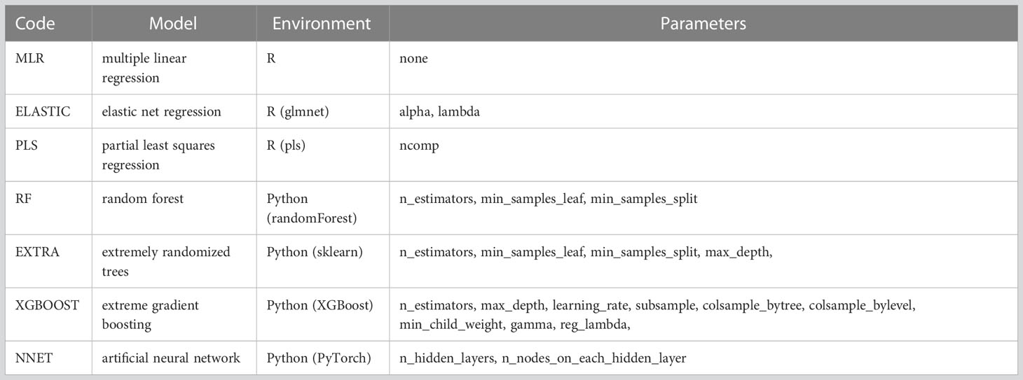
Table 2 Machine learning models used in the study and associate tuned hyperparameters.

Linear regression is a straightforward algorithm based on supervised learning, where the predicted output is continuous and has a constant slope. It is one of the fundamental ML models due to its relative simplicity and clear properties. A multiple linear regression (MLR) model extends linear regression to several explanatory variables (Jobson, 1991). However, MLR loses efficiency when the number of explanatory variables is large or when the variables are highly correlated (collinear). Regularization techniques offer a solution to this problem by incorporating additional information or constraints into the model training process. The goal is to control the complexity of the model and to reduce the potential for overfitting. During training, a penalty term is added to the loss function, encouraging smaller coefficient values and mitigating the impact of correlated variables. There are two main types of regularization techniques: ridge regression and lasso regression. Ridge regression is effective for handling multicollinearity as it adds an L2 penalty term, penalizing the sum of squared coefficients. This encourages the model to distribute the influence of the explanatory variables across all features, reducing the dominance of any single variable. On the other hand, lasso regression applies an L1 penalty, driving some coefficients exactly to zero by penalizing the sum of their absolute values. This sparsity-inducing property makes lasso regression useful for feature selection and identifying the most important variables in the model. By pushing the coefficient of correlated variable towards zero, lasso regression results in fewer features being included in the final model while still preserving relevant regression information. Elastic net regression (ELASTIC) is a regularized regression method that combines both the L1 and L2 penalties of the lasso and ridge methods. In addition to regularization, dimensionality reduction techniques such as partial least squares regression (PLS) can seek a lower-dimensional representation of the features that retains essential relationships in the data. PLS achieves this by projecting the predicted and observable variables into a new space, extracting factors that capture most of the variation in the response (Vinzi et al., 2010).

We also investigated several non-linear ML methods that could probably better address climatic predictions. Regression trees (RT) are the regression version of decision trees (Breiman et al., 1984), which are ML algorithms that partition the data into subsets. RT are constructed by splitting training dataset into smaller subsets based on an attribute value test, which are then fitted along the tree branches. The partitioning process starts with binary split and proceeds until no further splits can be made, resulting to various tree paths of variable length. RT can handle high dimensional data, but they are prone to overfitting and can be unstable, as a slight change in the input dataset can greatly affect the predictions. Tree-based ensemble methods have emerged to improve the predictive power of decision trees. Ensemble methods involve using multiple trees and combining their results to produce a single optimal prediction. Random forest (RF) models aggregate an ensemble of successive fully-grown individual regression trees, which are decision trees expanded until each leaf node contains only one data point or all data points in the node share the same target value (Breiman, 2001). This allows the trees to capture intricate relationships and potential overfitting to the training data. The random forest model is trained through bootstrap aggregating, also known as bagging, which involves creating multiple subsets of the original training data by randomly sampling with replacement. Each subset, called a bootstrap sample, is of the same size as the original dataset but may include duplicate instances and exclude some instances. Extremely randomized trees (EXTRA) are similar to RF, but they do not resample observations when building a tree and use a small number of randomly chosen splits-points for each of the selected predictors (Geurts et al., 2006). Extreme gradient boosting (XGBOOST) is a gradient boosting algorithm, i.e., an ensemble model that fits consecutive weak trees, also known as shallow decision trees, on the residuals from the previous iterations. These weak trees have limited depth or complexity and are combined using a gradient descent algorithm to minimize the fitting errors in each iteration of the boosting process.(T. Chen and Guestrin, 2016). An Artificial Neural Network (NNET) is based on interconnected units called artificial neurons that are typically arranged in a series of layers (Haykin, 1999). Each neuron receives input from the neurons on the previous layer, undergoes a weighted transformation of this input, and sends an output signal to the neurons of the next layer. The weights assigned to the connections between neurons represent the strengths or importance of the respective inputs. During the training process, these weights are adjusted iteratively using optimization algorithms that minimize the difference between the network’s predicted outputs and the actual targets. This adjustment of weights enables the network to learn complex patterns and relationships in the training data, allowing it to make predictions on new, unseen inputs based on the learned patterns. A Deep Learning Network refers to a NNET architecture that uses multiple layers of neurons to extract higher-level features from the raw input.

All analyses were performed using R 4.0.2 (R Core Team, 2020) and Python 3.8.8 (van Rossum and Drake, 2009), using various packages and libraries for model fitting and parameterisation (Table 2). The R and Python scripts for our analyses are provided in the supplementary material.

2.2.1 Model configuration

Each ML model has specific internal parameters, called hyperparameters, which help to control the learning process for a given problem. Different ML algorithms require different hyperparameters, e.g., number of trees in random forests or the number of hidden layers and units in artificial neural networks, which must be set before training. In this study, we used grid search and randomized search with cross-validation for hyperparameter optimization according to the trained model. The selected hyperparameters that were tuned for each model are provided in Table 2.

2.2.2 Model validation

This study utilized geographically-based partitioning to create training/validation and test sets with a 0.75 partitioning ratio. The aim was to address spatial autocorrelation and to prevent excessive similarity between observations used during training and test phases, ensuring their statistical independence (Dormann et al., 2007). Certain geographical areas exhibit low internal climatic variability as well as homogeneity in their faunal community composition. This effect is likely to be more pronounced in regions characterized by low species richness. In a random split, selecting neighboring locality observations for training and validation will thus result in dependencies. To tackle this issue, the entire data was partitioned into geographically distributed blocks across Africa (Figure 2), with continuous latitudinal and longitudinal bands serving as dividers (see other strategies to account for spatial autocorrelation in Dormann et al., 2007; Wenger and Olden, 2012; Le Rest et al., 2014; Roberts et al., 2017; Mendoza and Araujo, 2022). The size of the blocks (2.1 x 2.1 degrees) was determined to achieve a balance between accommodating species with limited geographic ranges and providing sufficient coverage for evaluating the models’ adaptability to climatic conditions without direct analogues. Approximately 75% of the dataset was encompassed within the blocks, constituting the training set, while the remaining 25% of observations within the latitudinal and longitudinal bands formed the test set. These bands introduce disruptions in the geographical continuity observed in the blocks that will be employed for cross-validation. To assess model performance and optimize the hyperparameters of models over grid searches, the geographical blocks were then randomly assigned to five folds for cross-validation, using one fold for testing and the remaining four folds for model fitting. After the process is iterated until the five folds have been used for testing once, we calculated the average performance metrics (details below) across the five iterations in order to estimate the model’s generalization performance (summarized in Table S1). Finally, we selected the best-performing model based on the average performance and used it to make predictions on unseen test data.

FIGURE 2

Figure 2 The dataset was divided into a training set, consisting of non-adjacent blocks distributed uniformly (75% of the data, in blue), and a test set (25% of the data, in pink). Blocks from the training set were assigned randomly to five folds, each marked with a distinct color that shows allocation of blocks to folds, for 5-fold cross validation.

Although this strategy limits sources of error and bias in the predictions, it is worth mentioning that autocorrelation cannot be fully addressed satisfactorily in our presence–absence design problem, for occurrences are highly imbalanced between species: for instance, the distribution of the Natal multimammate mouse Mastomys natalensis covers almost all Africa south of the Sahelian zone, while Issel’s groove-toothed swamp rat Pelomys isseli is restricted to a few islands in Lake Victoria. This situation leads to blocks lacking either presences or absences, which will affect the model’s ability to generalize patterns effectively. To assess the predictive performance of the fitted models, we used root mean square error (RMSE), mean absolute error (MAE), coefficient of determination (R²) and adjusted coefficient of determination (aR²) metrics. RMSE, MAE, R², and aR² are calculated as follows:

$$RMSE= \sqrt{\frac{1}{N}\sum _{ i=1}^N\left(y_i-\widehat{y} \right)2}$$

$$MAE= \frac{1}{N}\sum _{ i=1}^N|y_i-\widehat{y}|$$

$$R^2=1-\frac{\sum \left(y_i-\widehat{y} \right)2}{\sum \left(y_i-\overline{y} \right)2}$$

$$a{R}^2=1-\frac{\left(1-R^2\right)\left(N-1\right)}{N-p-1}$$

where N is the number of samples for validation, y_i, $\widehat{y}$ and $\overline{y}$ are observed, predicted and mean values of y respectively, and p is the number of input variables (predictors). RMSE is the square root of MSE, which represents the average of the squared difference between the original and predicted values; it measures the standard deviation of the residuals. MAE represents the average magnitude of the differences between the original and predicted values, regardless of the direction of the errors. R² represents the proportion of variance for a dependent variable that is explained by an independent variable; it is a scale-free score, represented as a value between 0 and 1. The adjusted R² is a modification of the R² that penalizes the inclusion of unnecessary predictors in a regression model, providing a more conservative estimate of the model’s performance while accounting for its complexity. It is a measure that balances the goodness of fit with the number of predictors. RMSE, MAE,R², and aR² are four common of many quantifiable ways to check how predicted values are closely related to actual observed values (Chai and Draxler, 2014).

2.2.3 Model interpretation

Variable importance, also called feature importance, allows ranking the relative contributions of input variables for predicting the output variable (Friedman, 2001). It also provides an interesting global insight into the model’s behavior. There are many methods to compute variable importance scores in a fitted model, some model-specific, others model-independent (e.g., Archer and Kimes, 2008; Williamson et al., 2021). In this contribution, Random Forests (RF) demonstrated superior predictive performance compared to other models, leading us to focus on this algorithm. To assess the importance of variables, we used a built-in feature importance evaluation from the RF algorithms, which is based on the mean decrease in residual sum of squares (Breiman, 2001).

2.3 Testing the models on new faunal datasets

As the dataset on which the models have been trained is derived from range maps rather than point-occurrence records, predictions are based on a scenario of full occurrence of the maximum possible species on each cell. For example, the highest species richness is found in the Central African rainforest with a total of 62 sympatric species. In practice, however, faunal data from field inventories or archeological excavations rarely represent exhaustive inventories. There is much variety when it comes to survey (e.g. owl pellet counts, pitfall and snap traps, acoustic techniques, camera surveys), with a potential impact on sampling efficiency that can alter richness and abundance estimates (Andrews, 1990; Umetsu et al., 2006). To ensure the reliability of climatic inferences and their extrapolation to local rodent surveys where sample success is lower, trained models were tested on eight faunal lists derived from published rodent surveys from various African countries (Table 3). These lists show discrepancies between the number of identified species and the theoretical maximal specific diversity according to the literature. Climatic conditions predicted with the fitted models can then be compared with real local conditions, allowing estimating the reliability of our method. Of course, it is not expected that predictions from a small number of species will exactly match climatic records at the eight locations; however, the comparison of actual and predicted bioclimatic values can be viewed as an easy “test case” and a first demonstration of the exportability of our methods to no-analog small mammal communities.

FIGURE 3

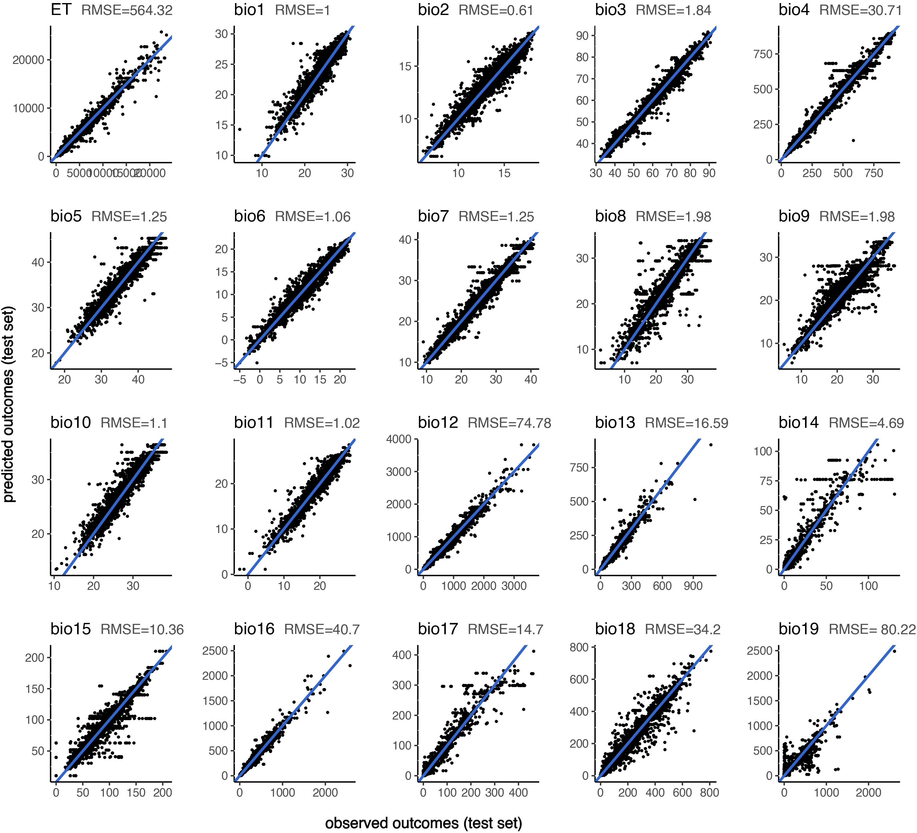
Figure 3 Actual (observed) and predicted values of the 20 bioclimatic variables for the test data set (n = 89420) with the random forest model.

TABLE 3

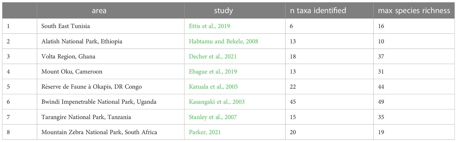
Table 3 List of published rodent inventories from various African localities, with the number of identified taxa (various taxonomic ranks included) used in the predictions and the theoretical maximum number of species at this location based on the literature.

To visually identify the areas with the highest similarity in terms of climatic conditions to the predictions derived from faunal lists, maps have been generated by rasterizing the Euclidean distance values between the output vector containing the 20 predicted variables and each cell of the dataset.

3 Results

3.1 Performance of ML models

Performances of the seven algorithms for predicting the 20 target climatic variables after cross-validation are shown in Table 4 (RMSE and aR²) and Supplementary Table 1 (MAE and R²). Each of the non-linear ML models achieved substantially better prediction performances than the linear models. The highest performing model is RF, closely followed by XGBOOST and NNET, based on the RMSE and aR² values on the test set. The lowest performing model is PLS, regardless of the output variable. Relationship between the observed and predicted outcomes using RF models on test setare illustrated with scatter plots for each variable in Figure 3. There are also differences in the models’ performances with respect to the predicted output variable: evapotranspiration (ET), annual precipitation (bio12) and temperature seasonality (bio4) are consistently predicted very accurately (aR² = 0.98 for the three variables with RF model); by contrast, the mean temperature of the driest quarter (bio9) and the precipitation of the coldest quarter (bio19) are the most difficult variables to predict using the faunal input variables. Based on these scores, we adopted the random forest (RF) as the most efficient ML regression model for the rest of the analysis.

TABLE 4

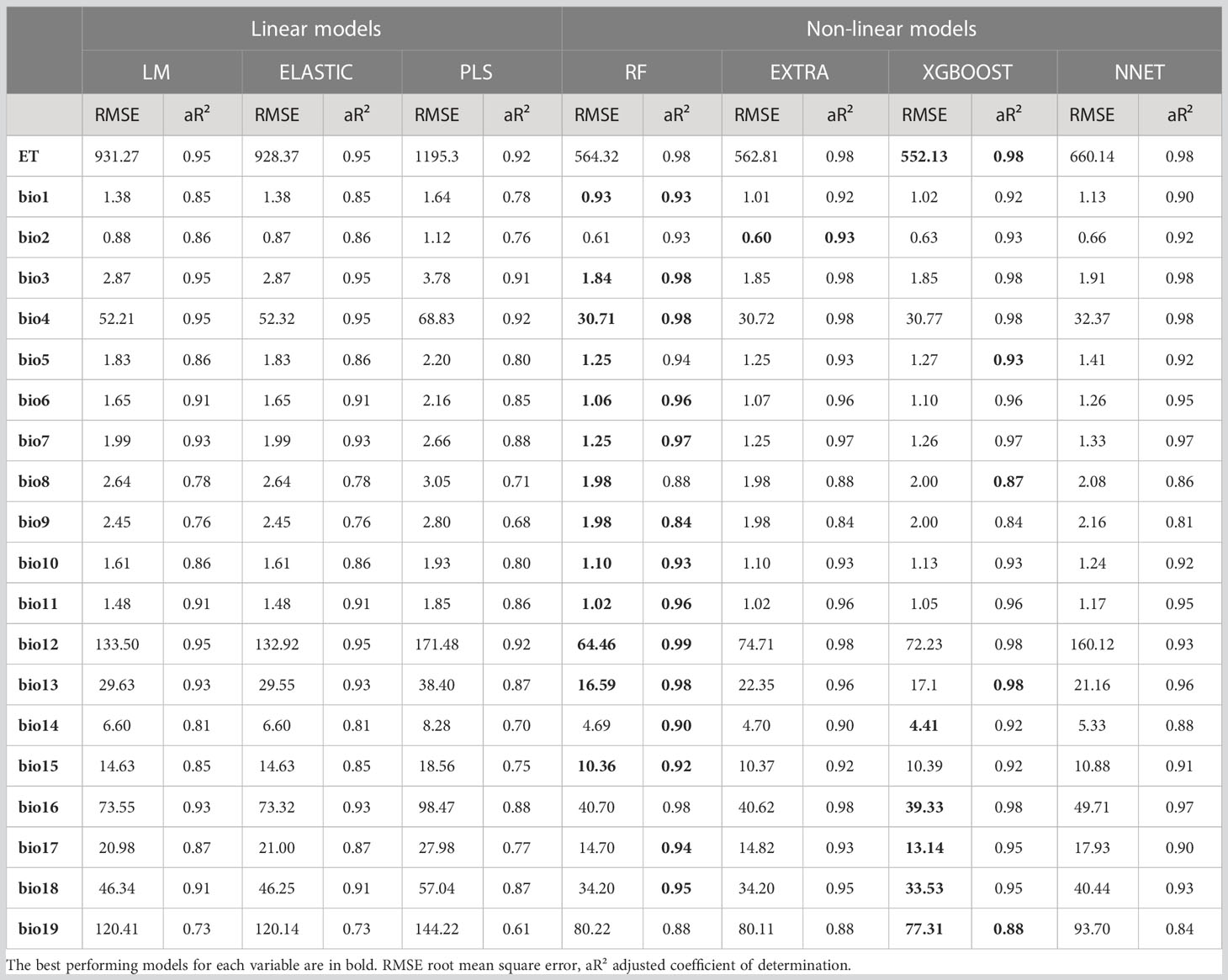
Table 4 Performance evaluation of ML regression methods.

FIGURE 4

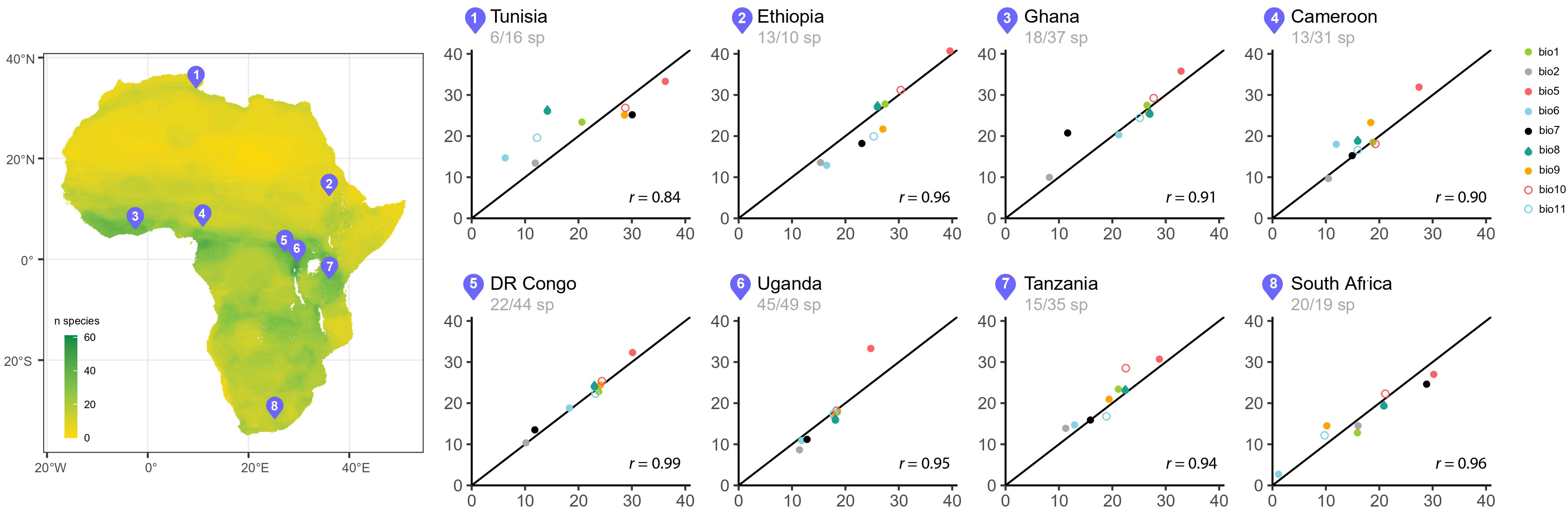
Figure 4 On the left, map of Africa showing rodent species richness and the location of eight nature reserves associated with rodent surveys (see Table 3 for the references of the locations); on the right, scatter plots of observed and predicted values for nine temperature variables using RF algorithm based on each rodent survey. The black diagonal line represents the line of perfect prediction. The numbers under the countries correspond to the number of species identified in the publication and therefore used for the predictions/theoretical maximum number of species at the same location.

3.2 Climatic predictions on new dataset

RF-based prediction of the distinct bioclimatic conditions from several published rodent lists (details in Table 3) provided results that are in most cases matching closely with records from weather stations around the areas. Figure 4 shows the predictions from the RF models for nine temperature parameters compared to the temperature records from the climate stations in the study areas.

There is a high correspondence between the observed temperature records from the weather stations and the values of temperature variables predicted by the RF algorithms based on the rodent lists. This is all the more striking, since these inferences are made with original faunal data beyond the data set used for model fitting.

4 Discussion

4.1 Nonlinear vs. linear models

Unsuprisingly, all the nonlinear ML models consistently provided better performances than the linear models. In particular, RF, XGBOOST, and NNET appear to be the most promising algorithms for predicting climatic variables based on the presence or absence of rodents. Unlike linear models, they are successful in capturing nonlinear patterns and interactions (Bishop, 2006). The actual spatial limits of distribution of rodent species are controlled by complex interactions between several biotic (e.g., competition, predation, vegetation) and abiotic (e.g., soil nutrients, anthropogenic land-use change, water availability, fires, etc.) factors. As a result, bioclimatic factors can drive differential responses on the abundance and presence of some species that can hardly be captured by linear statistical models. This is not particularly surprising, as similar observations were also made for other climate predictions with ML based on pollen samples (Salonen et al., 2019; Sobol et al., 2019). The corollary to this is that RF identified important contributing taxa that were not or were little considered by linear models, such as the genera Euxerus or Hystrix for predicting annual mean temperature (see Figure 5). This provides an example of how non-linear models captured more detailed effects that allow to better characterize the climatic components of an environment. However, an overly sophisticated, complex statistical model may be prone to overfitting; this occurs when a model fits exactly against its training data and learns detail and noise to the extent that it negatively impacts its performances on unseen data (Dietterich, 1995; Hawkins, 2004). It is nevertheless possible to avoid overfitting bias in several ways such as using cross-validation, backtesting, regularization or by carefully tuning the hyperparameters pertaining to the model.

FIGURE 5

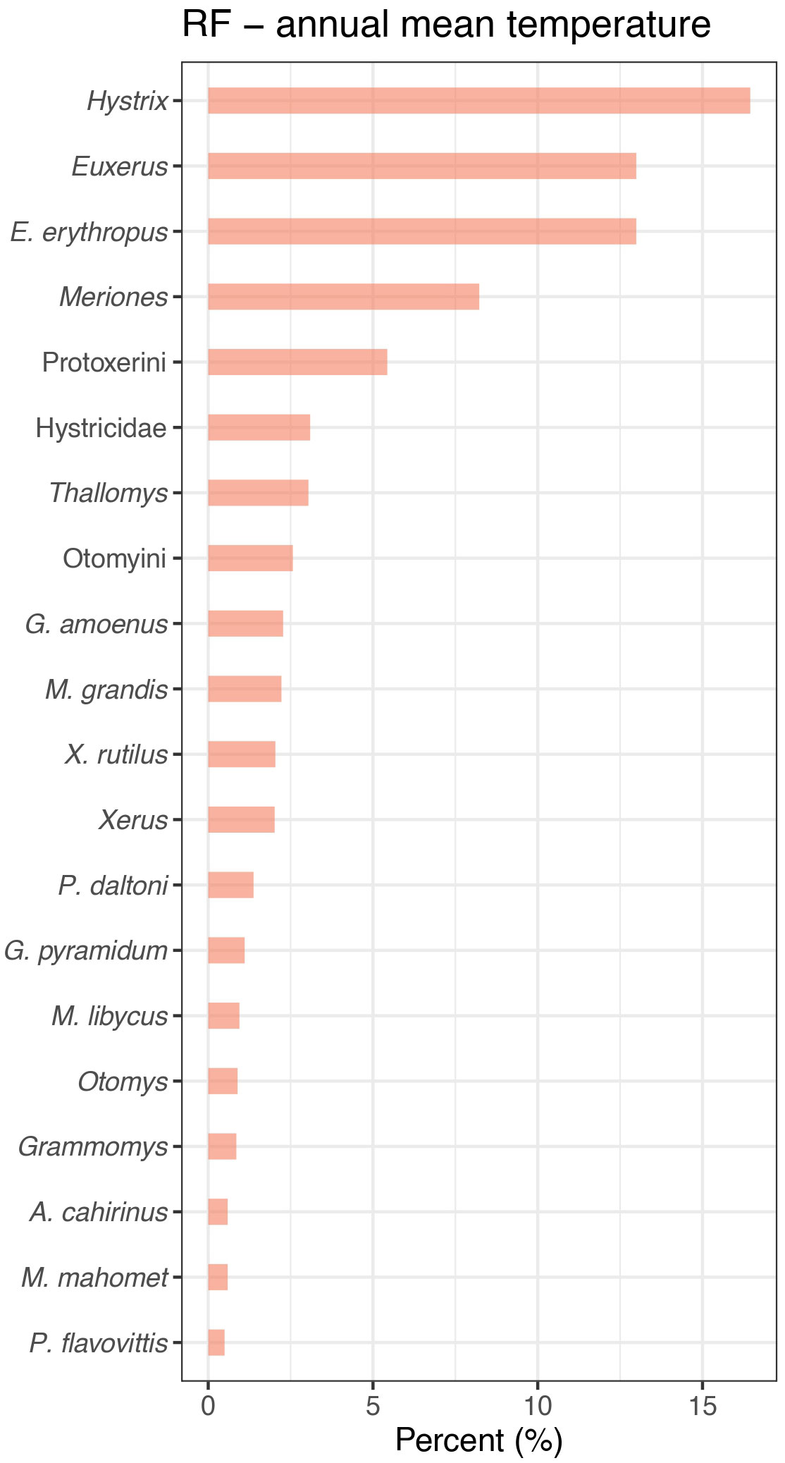
Figure 5 Comparison of the 20 most important relative variables of the random forest (RF) model used to predict the annual mean temperature (bio1).

4.2 Performance of the RF algorithm

Using tree-based ensemble methods, we successfully predicted bioclimatic components of multiple African environments based on rodent communities. Although the actual distribution of most rodent species is driven by many environmental and anthropogenic factors that are hardly quantifiable (including type and density of vegetation, soil physical characteristics, elevation, predator status, farm management practices, for instance), rodents are primary consumers with strict ecological requirements for most of them; thus, we were expecting to predict bioclimatic variables with a fair degree of accuracy. The striking performance achieved by our RF models provides support for the contribution of ML approaches to predictive environmental modelling from species distribution.

The set of 19 bioclimatic variables from Worldclim is derived from monthly temperature (minimum and maximum temperatures) and rainfall values. Our models achieved the best performances for primary variables that derive directly from these values, such as annual precipitation, temperature seasonality, precipitation of the wettest quarter, etc. By contrast, predicted variables for which we obtained more mixed performances are secondary variables, i.e., combinations of the temperature and precipitation values, such as mean temperature of wettest quarter, precipitation of coldest quarter, and mean temperature of driest quarter. This can have a significant impact on depicting climate or environment when one chooses to select for any reason only a few response variables.

One of the advantages of the RF regression algorithm is the possibility of easily including many covariates with minimal tuning (see Table 2) and supervision in comparison with other nonlinear methods such as XGBOOST or NNET. However, there are several obstacles that may hamper the accuracy and performance of our models. The most obvious one relates to the reliability of species distribution data. As a rule, the geographic range for widespread species is less precise than for species with restricted distributions. This may result in a further overrepresentation of widespread taxa in the dataset (with an impact on the relative important variables for each model) and mask the distribution of species along climatic gradients. By using range maps instead of observed points of occurrence, however, it will be easy to quickly refine predictor variables as more detailed data on rodent species occurrence will be available in the future. In addition, although no less than 463 species of African rodents were used as predictors, this large number of variables may still be insufficient for highly accurate climate modelling at the scale of the entire African continent. In the wild, the same association of rodent species can occur in different places with different climatic characteristics. Among the 350k localities recorded in our dataset, around 40% only display a unique combination of occurring species, while the remaining 60% of the localities have one or more replicates. This is especially the case for environments with low specific diversity, such as the central Sahara or the Namib Desert, for example.

4.3 Paleoclimate reconstruction

Our method using RF algorithm has strong potential to be used as new quantitative paleoclimate and paleoenvironmental reconstruction tool from fossil data. The discovery of new paleontological and archeological deposits is continuing apace, which often yield abundant and well-preserved faunal fossil remains that constitute the prime material for describing past environmental conditions. Our method may provide additional details on paleoenvironmental conditions within which such fossil assemblages were accumulated and deposited by retrodicting primary and secondary variables independently with a great performance.

The aggregation of spatial data in the initial dataset allows to produce visually impactful similarity maps to compare predicted environments with the current environmental conditions (see Figure 6). In the context of reconstructing fossil hominid environments, for instance, these maps could illustrate potential dispersal routes or paleodistribution maps.

FIGURE 6

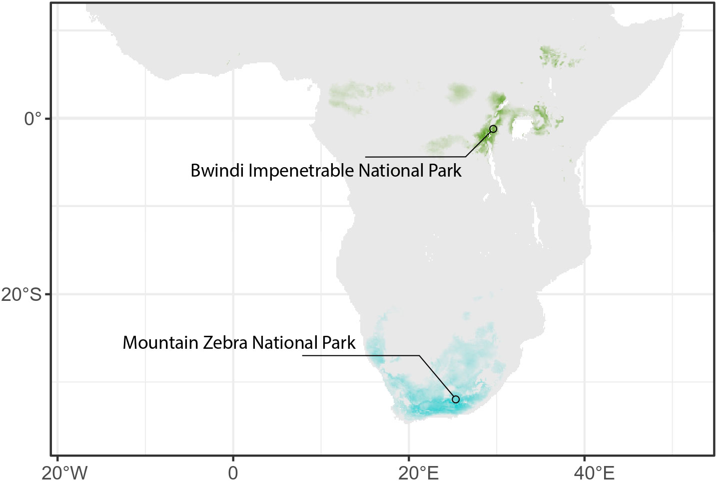
Figure 6 Map of Africa showing areas with bioclimatic conditions analogous to those predicted by RF algorithms based on the list of rodents from Mountain Zebra National Park, South Africa (in blue), and from Bwindi Impenetrable National Park, Uganda (in green). Areas of more intense colors indicate highest climatic similarity.

The capacity of our models for coping with heterogeneous taxonomic distinction may also help to refine ecological inferences based on published faunal lists. In archeological and paleontological context, fossils are not always identifiable at the species level using traditional morphological characters. For instance, the smallest species of rodents such as Mus, Dendromus or Graphiurus species can be hard to identify due to higher fragmentation rate in sediments and the lack of patent specific dental or cranial characters (Linchamps et al., 2021). The task is even more complicated for remote periods for which few comparative specimens are available. With fossil assemblages where such problems occur, only methods that consider variable taxonomic resolution are useful for faithful paleoclimate reconstruction. Calculating the most important variables that contribute to the overall prediction showed that not only the species level, but also the broader taxonomic levels, such as the subfamily or the family (see Figure 5), can be particularly indicative for modeling the climatic components of an environment.

It is assumed that confidence in the validity and performance of a paleoenvironmental reconstruction usually decreases as the faunal assemblage examined is older (Avery, 2007; Reed, 2007; Lyman, 2017). This is primarily due to the potential evolutionary changes in species’ tolerances over time, which may introduce uncertainty into the reconstructions. Holocene and Upper Pleistocene faunal collections therefore usually provide the most accurate and reliable interpretations, while the Quaternary faunas, characterized by the emergence and establishment of modern lineages, may still offer a reliable requisite degree of temporal distance. To check how well do our RF models perform with fossil data, predicted values could be compared with those from other quantitative methods independent of the taxonomy such as isotopic analyses (e.g. Cerling et al., 1997; Garrett et al., 2015), ecomorphology (e.g. Kovarovic and Andrews, 2007; Plummer et al., 2015) or teeth meso- and micro-use wear (e.g. Hopley et al., 2006). Combining medium and large fauna would also give a more comprehensive signal. Due to different modes of accumulation, micromammals and larger mammals are seldom fossilized together, although they coexisted (Andrews, 1990; Fernández-Jalvo and Andrews, 2016). It can therefore be difficult to link different taxonomic groups as taphonomic biases may have favored the over-representation of one group. This issue comes up frequently among researchers, and the most successful attempts at a holistic approach often involve laborious and time-demanding crossing of the disciplines in paleosciences (Lotter, 2005). At the same time, future knowledge of the distribution and habitats of extinct species for which little information is available may result in better integration of fossil taxa.

Although this method can deal with uncertainties in taxonomic identification, it would still require data from clear stratigraphic context with a proper sampling effort to ensure the representativeness of the mammal community. In this perspective, some taphonomic calibration tools would benefit from being combined with our method for finer paleoenvironmental interpretations. In the case of vertebrate accumulations, various taphonomic processes may alter the faunal composition from living to dead to fossil assemblage, such as predation, breakage, or dispersion of bones (Brain, 1981; Behrensmeyer, 1984; Andrews, 1990). A way to adapt the method to these particular conditions is to define various exclusion thresholds for taxa not likely to occur in a specific context, based on expert knowledge.

5 Conclusions

In this study, we develop a new well-performing method for bioclimatic predictions using faunal communities as proxy data with a ML regression approach. Among the different algorithms, the random forest regression algorithm provided the highest performance in predicting bioclimatic variables. Our standardized protocol for compiling and processing mammal distribution data as input source for environmental predictions allowed us to overcome traditional obstacles in faunal-based climate reconstructions related to the incompleteness and heterogeneity of the sample. This approach has the potential to be a useful tool for landscape and climate reconstructions of paleontological and archeological sites where faunal remains are available. It may further be generalized to embed other important types of environmental archives for even finer climatic reconstructions.

Data availability statement

Publicly available datasets were analyzed in this study. This data can be found here: R and Python codes related to this paper were archived with Figshare at https://figshare.com/s/740b9a6cdf1f5a2a7e3a. Species distribution maps can be found at https://www.iucnredlist.org/ (accessed on 1st of February 2023) and at https://mol.org/ (accessed on 1st of February 2023) for the different African rodent species. Bioclimatic variables can be found at https://worldclim.org/data/bioclim.html (accessed on 1st of February 2023). The evapotranspiration variable is available at https://cgiarcsi.community (accessed on 1st of February 2023).

Author contributions

PLi, RH, FR, PLa and RC conceived the ideas and designed methodology. PLi collected and analyzed the data. ES helped supervise the project. PLi led the writing of the manuscript. All the authors contributed critically to the drafts and gave final approval for publication. All authors contributed to the article and approved the submitted version.

Acknowledgments

We would like to acknowledge Fayçal Allouti (Muséum national d’Histoire naturelle) and the intensive computing platform « Plateforme de Calcul Intensif et Algorithmique PCIA, Muséum national d’Histoire naturelle, Centre national de la recherche scientifique, UAR 2700 2AD, CP 26, 57 rue Cuvier, F-75231 Paris Cedex 05, France » for allowing model training. We also thank Maël Doré (Muséum national d’Histoire naturelle) for his help and useful comments that enhanced the quality of this work.

Conflict of interest

The authors declare that the research was conducted in the absence of any commercial or financial relationships that could be construed as a potential conflict of interest.

Publisher’s note

All claims expressed in this article are solely those of the authors and do not necessarily represent those of their affiliated organizations, or those of the publisher, the editors and the reviewers. Any product that may be evaluated in this article, or claim that may be made by its manufacturer, is not guaranteed or endorsed by the publisher.

Supplementary material

The Supplementary Material for this article can be found online at: https://www.frontiersin.org/articles/10.3389/fevo.2023.1178379/full#supplementary-material

References

Andrews P. (1990). Owls, caves and fossils: predation, preservation and accumulation of small mammal bones in caves, with an analysis of the pleistocene cave faunas from westbury-Sub-Mendip (Somerset, U.K: University of Chicago Press).

Google Scholar

Andrews P. (1995). Mammals as palaeoecological indicators. Acta Zool. Cracoviensia 38, 1.

Google Scholar

Andrews P., Hixson S. (2014). Taxon-free methods of palaeoecology. Annales Zoologici Fennici 51, 269–284. doi: 10.5735/086.051.0225

CrossRef Full Text | Google Scholar

Andrews P., Reynolds S. C., Bobe R. (2022). “Approaches to the study of past environments,” in African Paleoecology and human evolution. Eds. Bobe R., Reynolds S. C. (Cambridge: Cambridge University Press). doi: 10.1017/9781139696470.002

CrossRef Full Text | Google Scholar

Archer K. J., Kimes R. V. (2008). Empirical characterization of random forest variable importance measures. Comput. Stat Data Anal. 52 (4), 2249–2260. doi: 10.1016/j.csda.2007.08.015

CrossRef Full Text | Google Scholar

Avery D. M. (2001). The plio-pleistocene vegetation and climate of sterkfontein and swartkrans, south Africa, based on micromammals. J. Hum. Evol. 41 (2), 113–132. doi: 10.1006/jhev.2001.0483

PubMed Abstract | CrossRef Full Text | Google Scholar

Avery D. M. (2007). Micromammals as palaeoenvironmental indicators of the southern African quaternary. Trans. R. Soc. South Afr. 62 (1), 17–23. doi: 10.1080/00359190709519193

CrossRef Full Text | Google Scholar

Bartlein P., Harrison S., Brewer S., Connor S., Davis B., Gajewski K., et al. (2011). Pollen-based continental climate reconstructions at 6 and 21 ka: a global synthesis. Climate Dyn. 37, 775–802. doi: 10.1007/s00382-010-0904-1

CrossRef Full Text | Google Scholar

Beery S., Cole E., Parker J., Perona P., Winner K. (2021). “Species distribution modeling for machine learning practitioners: a review,” in ACM SIGCAS Conference on Computing and Sustainable Societies (COMPASS) (COMPASS ’21); June 28–July 2, 2021; Virtual Event, Australia. New York, NY, USA: ACM. doi: 10.1145/3460112.3471966

CrossRef Full Text | Google Scholar

Behrensmeyer A. K. (1984). Taphonomy and the fossil record: the complex processes that preserve organic remains in rocks also leave their own traces, adding another dimension of information to fossil samples. Am. Scientist 72 (6), 558–566.

Google Scholar

Bellinger C., Mohomed Jabbar M. S., Zaïane O., Osornio-Vargas A. (2017). A systematic review of data mining and machine learning for air pollution epidemiology. BMC Public Health 17 (1), 907. doi: 10.1186/s12889-017-4914-3

PubMed Abstract | CrossRef Full Text | Google Scholar

Bertrand R., Lenoir J., Piedallu C., Riofrío-Dillon G., de Ruffray P., Vidal C., et al. (2011). Changes in plant community composition lag behind climate warming in lowland forests. Nature 479, 7374. doi: 10.1038/nature10548

CrossRef Full Text | Google Scholar

Birks H., Heiri O., Bjune A. (2010). Strengths and weaknesses of quantitative climate reconstructions based on late-quaternary biological proxies. Open Ecol. J. 3, 68–110. doi: 10.2174/1874213001003020068

CrossRef Full Text | Google Scholar

Bishop C. M. (2006). Pattern recognition and machine learning (New York: Springer).

Google Scholar

Blain H.-A., Bailon S., Cuenca-Bescós G., Arsuaga J. L., Bermúdez de Castro J. M., Carbonell E. (2009). Long-term climate record inferred from early-middle pleistocene amphibian and squamate reptile assemblages at the gran dolina cave, atapuerca, Spain. J. Hum. Evol. 56 (1), 55–65. doi: 10.1016/j.jhevol.2008.08.020

PubMed Abstract | CrossRef Full Text | Google Scholar

Botella C., Joly A., Bonnet P., Monestiez P., Munoz F. (2018). “A deep learning approach to species distribution modelling,” in Multimedia tools and applications for environmental and biodiversity informatics. Eds. Joly A., Vrochidis S., Karatzas K., Karppinen A., Bonnet P. (Cham: Springer International Publishing). doi: 10.1007/978-3-319-76445-0_10

CrossRef Full Text | Google Scholar

Brain C. K. (1981). The hunters or the hunted?: an introduction to African cave taphonomy (Chicago: University of Chicago Press).

Google Scholar

Breiman L. (2001). Random forests. Mach. Learn. 45 (1), 5–32. doi: 10.1023/A:1010933404324

CrossRef Full Text | Google Scholar

Breiman L., Friedman J. H., Olshen R. A., Stone C. J. (1984). Classification and regression trees (Boca Raton: Routledge).

Google Scholar

Cerling T. E., Harris J. M., MacFadden B. J., Leakey M. G., Quade J., Eisenmann V., et al. (1997). Global vegetation change through the Miocene/Pliocene boundary. Nature 389 (6647), 153–158. doi: 10.1038/38229

CrossRef Full Text | Google Scholar

Cerling T. E., Wynn J. G., Andanje S. A., Bird M. I., Korir D. K., Levin N. E., et al. (2011). Woody cover and hominin environments in the past 6 million years. Nature 476 (7358), 51–56. doi: 10.1038/nature10306

PubMed Abstract | CrossRef Full Text | Google Scholar

Chai T., Draxler R. R. (2014). Root mean square error (RMSE) or mean absolute error (MAE)? – arguments against avoiding RMSE in the literature. Geosci. Model. Dev. 7 (3), 1247–1250. doi: 10.5194/gmd-7-1247-2014

CrossRef Full Text | Google Scholar

Chen J., de Hoogh K., Gulliver J., Hoffmann B., Hertel O., Ketzel M., et al. (2019). A comparison of linear regression, regularization, and machine learning algorithms to develop Europe-wide spatial models of fine particles and nitrogen dioxide. Environ. Int. 130, 1–14. doi: 10.1016/j.envint.2019.104934

CrossRef Full Text | Google Scholar

Chen T., Guestrin C. (2016). “XGBoost: a scalable tree boosting system,” in Proceedings of the 22nd ACM SIGKDD International Conference on Knowledge Discovery and Data Mining. KDD ’16, August 13–17, 2016, San Francisco, CA, USA (arXiv:2107.10400v1), 785–794. doi: 10.1145/2939672.2939785

CrossRef Full Text | Google Scholar

Clavel J., Morlon H. (2017). Accelerated body size evolution during cold climatic periods in the Cenozoic. Proc. Natl. Acad. Sci. U.S.A. 114 (16), 4183–4188. doi: 10.1073/pnas.1606868114

PubMed Abstract | CrossRef Full Text | Google Scholar

Cui Z., Gong G. (2018). The effect of machine learning regression algorithms and sample size on individualized behavioral prediction with functional connectivity features. NeuroImage 178, 622–637. doi: 10.1016/j.neuroimage.2018.06.001

PubMed Abstract | CrossRef Full Text | Google Scholar

Damuth J., Janis C. (2011). On the relationship between hypsodonty and feeding ecology in ungulate mammals, and its utility in palaeoecology. Biol. Rev. Cambridge Philos. Soc. 86, 733–758. doi: 10.1111/j.1469-185X.2011.00176.x

CrossRef Full Text | Google Scholar

Decher J., Norris R., Abedi-Lartey M., Oppong J., Hutterer R., Weinbrenner M., et al. (2021). A survey of small mammals in the Volta region of Ghana with comments on zoogeography and conservation. Zoosystema 43, 253–281. doi: 10.5252/zoosystema2021v43a14

CrossRef Full Text | Google Scholar

Dietterich T. (1995). Overfitting and undercomputing in machine learning. ACM Comput. Surveys 27 (3), 326–327. doi: 10.1145/212094.212114

CrossRef Full Text | Google Scholar

Dormann C., McPherson J., Araújo M., Bivand R., Bolliger J., Carl G., et al. (2007). Methods to account for spatial autocorrelation in the analysis of species distributional data: a review. Ecography 30 (5), 609–628. doi: 10.1111/j.2007.0906-7590.05171.x

CrossRef Full Text | Google Scholar

Dueben P. D., Bauer P. (2018). Challenges and design choices for global weather and climate models based on machine learning. Geosci. Model. Dev. 11 (10), 3999–4009. doi: 10.5194/gmd-11-3999-2018

CrossRef Full Text | Google Scholar

Ebague G. M., Missoup A. D., Chung E. K., Tindo M., Denys C. (2019). Terrestrial small mammal assemblage from pellets of three sympatric owl species in the mount oku area (Northwest Cameroon), with implications for conservation. Bonn xool. Bull. 68 (1), 13–19. doi: 10.20363/BZB-2019.68.1.013

CrossRef Full Text | Google Scholar

Ettis K., Chammem M., Khorchani T. (2019). Biodiversity of rodents in the agro-systems of southeastern Tunisia: case of olive groves and fields of barley. J. New Sci. 62, 3924–3931.

Google Scholar

Fagoaga A., Blain H.-A., Marquina-Blasco R., Laplana C., Sillero N., Hernández C. M., et al. (2019). Improving the accuracy of small vertebrate-based palaeoclimatic reconstructions derived from the mutual ecogeographic range. a case study using geographic information systems and UDA-ODA discrimination methodology. Quaternary Sci. Rev. 223, 1–12. doi: 10.1016/j.quascirev.2019.105969

CrossRef Full Text | Google Scholar

Fernández-Jalvo Y., Andrews P. (2016). Atlas of taphonomic identifications: 1001+ images of fossil and recent mammal bone modification (New York: Springer). doi: 10.1007/978-94-017-7432-1

CrossRef Full Text | Google Scholar

Fernández-Jalvo Y., Denys C., Andrews P., Williams T., Dauphin Y., Humphrey L. (1998). Taphonomy and palaeoecology of olduvai bed-I (Pleistocene, Tanzania). J. Hum. Evol. 34 (2), 137–172. doi: 10.1006/jhev.1997.0188

PubMed Abstract | CrossRef Full Text | Google Scholar

Fick S. E., Hijmans R. J. (2017). WorldClim 2: new 1-km spatial resolution climate surfaces for global land areas. Int. J. Climatol. 37 (12), 4302–4315. doi: 10.1002/joc.5086

CrossRef Full Text | Google Scholar

Friedman J. H. (2001). Greedy function approximation: a gradient boosting machine. Ann. Stat 29 (5), 1189–1232. doi: 10.1214/aos/1013203451

CrossRef Full Text | Google Scholar

Garrett N. D., Fox D. L., McNulty K. P., Faith J. T., Peppe D. J., Van Plantinga A., et al. (2015). Stable isotope paleoecology of late pleistocene middle stone age humans from the lake Victoria basin, Kenya. J. Hum. Evol. 82, 1–14. doi: 10.1016/j.jhevol.2014.10.005

PubMed Abstract | CrossRef Full Text | Google Scholar

Geurts P., Ernst D., Wehenkel L. (2006). Extremely randomized trees. Mach. Learn. 63 (1), 3–42. doi: 10.1007/s10994-006-6226-1

CrossRef Full Text | Google Scholar

Gibson P. B., Chapman W. E., Altinok A., Delle Monache L., DeFlorio M. J., Waliser D. E. (2021). Training machine learning models on climate model output yields skillful interpretable seasonal precipitation forecasts. Commun. Earth Environ. 2 (1), 159. doi: 10.1038/s43247-021-00225-4

CrossRef Full Text | Google Scholar

Grayson D. (1981). A critical view of the use of archaeological vertebrates in paleoenvironmental reconstruction. J. Ethnobiol. 1, 28–38.

Google Scholar

Habtamu T., Bekele A. (2008). Habitat association of insectivores and rodents of alatish national park, northwestern Ethiopia. Trop. Ecol. 49, 1–11.

Google Scholar

Hawkins D. M. (2004). The problem of overfitting. J. Chem. Inf. Comput. Sci. 44 (1), 1–12. doi: 10.1021/ci0342472

PubMed Abstract | CrossRef Full Text | Google Scholar

Haykin S. S. (1999). Neural networks: a comprehensive foundation (Upper Saddle River: Prentice Hall).

Google Scholar

Hernández Fernández M. (2001). Bioclimatic discriminant capacity of terrestrial mammal faunas. Global Ecol. Biogeogr. 10 (2), 189–204. doi: 10.1046/j.1466-822x.2001.00218.x

CrossRef Full Text | Google Scholar

Hernández Fernández M. (2006). Rodent paleofaunas as indicators of climatic change in Europe during the last 125,000 years. Quaternary Res. 65, 308–323. doi: 10.1016/j.yqres.2005.08.022

CrossRef Full Text | Google Scholar

Hopley P. J., Latham A. G., Marshall J. D. (2006). Palaeoenvironments and palaeodiets of mid-pliocene micromammals from makapansgat limeworks, south Africa: a stable isotope and dental microwear approach. Palaeogeogr. Palaeoclimatol. Palaeoecol. 233 (3), 235–251. doi: 10.1016/j.palaeo.2005.09.011

CrossRef Full Text | Google Scholar

Hurlbert A. H., Jetz W. (2007). Species richness, hotspots, and the scale dependence of range maps in ecology and conservation. Proc. Natl. Acad. Sci. 104 (33), 13384–13389. doi: 10.1073/pnas.0704469104

CrossRef Full Text | Google Scholar

Hurlbert A. H., White E. P. (2005). Disparity between range map- and survey-based analyses of species richness: patterns, processes and implications. Ecol. Lett. 8 (3), 319–327. doi: 10.1111/j.1461-0248.2005.00726.x

CrossRef Full Text | Google Scholar

Jain P., Coogan S. C. P., Subramanian S. G., Crowley M., Taylor S., Flannigan M. D. (2020). A review of machine learning applications in wildfire science and management. Environ. Rev. 28 (4), 478–505. doi: 10.1139/er-2020-0019

CrossRef Full Text | Google Scholar

Jansen E., Overpeck J., Briffa K. R., Duplessy J.-C., Joos F., Masson-Delmotte V., et al. (2007). “Palaeoclimate,” in Climate change 2007: the physical science basis. contribution of working group I to the fourth assessment report of the intergovernmental panel on climate change. Eds. Solomon S., Qin D., Manning M., Chen Z., Marquis M., Averyt K. B., Tignor M. (Cambridge: Cambridge University Press).

Google Scholar

Jobson J. D. (1991). “Multiple linear regression,” in Applied multivariate data analysis: regression and experimental design. Ed. Jobson J. D. (New York: Springer). doi: 10.1007/978-1-4612-0955-3_4

CrossRef Full Text | Google Scholar

Jones P. D., Briffa K. R., Osborn T. J., Lough J. M., van Ommen T. D., Vinther B. M., et al. (2009). High-resolution palaeoclimatology of the last millennium: a review of current status and future prospects. Holocene 19 (1), 3–49. doi: 10.1177/0959683608098952

CrossRef Full Text | Google Scholar

Kasangaki A., Kityo R., Kerbis J. (2003). Diversity of rodents and shrews along an elevational gradient in bwindi impenetrable national park, south-western Uganda. Afr. J. Ecol. 41 (2), 115–123. doi: 10.1046/j.1365-2028.2003.00383.x

CrossRef Full Text | Google Scholar

Katuala P. G. B., Hart J. A., Hutterer R., Leirs H., Dudu A. (2005). Biodiversity and ecology of small mammals (Rodents and shrews) of the “Réserve de faune à okapis”, demo- cratic republic of the Congo. Belgian J. Zool. 135, 191–196.

Google Scholar

Knudby A., LeDrew E., Brenning A. (2010). Predictive mapping of reef fish species richness, diversity and biomass in Zanzibar using IKONOS imagery and machine-learning techniques. Remote Sens. Environ. 114 (6), 1230–1241. doi: 10.1016/j.rse.2010.01.007

CrossRef Full Text | Google Scholar

Kovarovic K., Andrews P. (2007). Bovid postcranial ecomorphological survey of the laetoli paleoenvironment. J. Hum. Evol. 52 (6), 663–680. doi: 10.1016/j.jhevol.2007.01.001

PubMed Abstract | CrossRef Full Text | Google Scholar

Krapp M., Beyer R. M., Edmundson S. L., Valdes P. J., Manica A. (2021). A statistics-based reconstruction of high-resolution global terrestrial climate for the last 800,000 years. Sci. Data 8 (1), 1–18. doi: 10.1038/s41597-021-01009-3

PubMed Abstract | CrossRef Full Text | Google Scholar

Kwok R. (2019). AI Empowers conservation biology. Nature 567 (7746), 133–134. doi: 10.1038/d41586-019-00746-1

PubMed Abstract | CrossRef Full Text | Google Scholar

Le Rest K., Pinaud D., Monestiez P., Chadoeuf J., Bretagnolle V. (2014). Spatial leave-one-out cross-validation for variable selection in the presence of spatial autocorrelation. Global Ecol. Biogeogr. 23 (7), 811–820. doi: 10.1111/geb.12161

CrossRef Full Text | Google Scholar

Linchamps P., Stoetzel E., Hanon R., Denys C. (2021). Neotaphonomic study of two tyto alba assemblages from Botswana: palaeoecological implications. J. Archaeol. Sci.: Rep. 38. doi: 10.1016/j.jasrep.2021.103085

CrossRef Full Text | Google Scholar

Lorenzen E. D., Nogués-Bravo D., Orlando L., Weinstock J., Binladen J., Marske K. A., et al. (2011). Species-specific responses of late quaternary megafauna to climate and humans. Nature 479 (7373), 359–364. doi: 10.1038/nature10574

PubMed Abstract | CrossRef Full Text | Google Scholar

Lotter A. (2005). “Multi-proxy climatic reconstructions,” in Global change in the Holocene (New York: Routledge).

Google Scholar

Lyman R. L. (2017). Paleoenvironmental reconstruction from faunal remains: ecological basics and analytical assumptions. J. Archaeol. Res. 25 (4), 315–371. doi: 10.1007/s10814-017-9102-6

CrossRef Full Text | Google Scholar

Lyons K. S., Amatangelo K. L., Behrensmeyer A. K., Bercovici A., Blois J. L., Davis M., et al. (2016). Holocene Shifts in the assembly of plant and animal communities implicate human impacts. Nature 529 (7584), 80–83. doi: 10.1038/nature16447

PubMed Abstract | CrossRef Full Text | Google Scholar

Marsh C., Sica Y., Burgin C., Dorman W., Anderson R., Mijares I., et al. (2022). Expert range maps of global mammal distributions harmonised to three taxonomic authorities. J. Biogeogr. 49, 1–14. doi: 10.1111/jbi.14330

CrossRef Full Text | Google Scholar

Matthews T., Marean C. W., Cleghorn N. (2020). Past and present distributions and community evolution of muridae and soricidae from MIS 9 to MIS 1 on the edge of the palaeo-agulhas plain (south coast, south Africa). Quaternary Sci. Rev. 235, 1–29. doi: 10.1016/j.quascirev.2019.05.026

CrossRef Full Text | Google Scholar

Matthews T., Rector A., Jacobs Z., Herries A. I. R., Marean C. W. (2011). Environmental implications of micromammals accumulated close to the MIS 6 to MIS 5 transition at pinnacle point cave 9 (Mossel bay, Western cape province, south Africa). Palaeogeogr. Palaeoclimatol. Palaeoecol. 302, 3–4. doi: 10.1016/j.palaeo.2011.01.014

CrossRef Full Text | Google Scholar

Mendoza M., Araujo M. B. (2022). Biogeography of bird and mammal trophic structures. Ecography 2022 (7), 1–13. doi: 10.1111/ecog.06289

CrossRef Full Text | Google Scholar

Mendoza M., Janis C., Palmqvist P. (2005). Ecological patterns in the trophic-size structure of large mammal communities: a “taxon-free” characterization. Evol. Ecol. Res. 7, 505–530.

Google Scholar

Mondanaro A., Di Febbraro M., Melchionna M., Maiorano L., Di Marco M., Edwards N. R., et al. (2021). The role of habitat fragmentation in pleistocene megafauna extinction in Eurasia. Ecography 44 (11), 1619–1630. doi: 10.1111/ecog.05939

CrossRef Full Text | Google Scholar

Nogués-Bravo D., Rodríguez-Sánchez F., Orsini L., de Boer E., Jansson R., Morlon H., et al. (2018). Cracking the code of biodiversity responses to past climate change. Trends Ecol. Evol. 33 (10), 765–776. doi: 10.1016/j.tree.2018.07.005

PubMed Abstract | CrossRef Full Text | Google Scholar

Parker D. M. (2021). Mammals in the mountains: an historical review and updated checklist of the mammals of the mountain zebra national park. Koedoe 63 (1), 1–10. doi: 10.4102/koedoe.v63i1.1683

CrossRef Full Text | Google Scholar

Plummer T. W., Ferraro J. V., Louys J., Hertel F., Alemseged Z., Bobe R., et al. (2015). Bovid ecomorphology and hominin paleoenvironments of the shungura formation, lower omo river valley, Ethiopia. J. Hum. Evol. 88, 108–126. doi: 10.1016/j.jhevol.2015.06.006

PubMed Abstract | CrossRef Full Text | Google Scholar

R Core Team (2020). R: a language and environment for statistical computing (Vienna, Austria: R Foundation for Statistical Computing). Available at: https://www.eea.europa.eu/data-and-maps/indicators/oxygen-consuming-substances-in-rivers/r-development-core-team-2006.

Google Scholar

Reed D. N. (2007). “Serengeti micromammals and their implications for Olduvai paleoenvironments”, in Hominin Environments in the East African Pliocene. Eds. Bobe R., Alemseged Z., Behrensmeyer A. (New York: Springer).

Google Scholar

Reed K., Spencer L., Rector A. L. (2013). Faunal approaches in early hominin paleoecology. Early Hominin Paleoecol., 3–34. doi: 10.5876/9781607322252:C01

CrossRef Full Text | Google Scholar

Roberts D. R., Bahn V., Ciuti S., Boyce M. S., Elith J., Guillera-Arroita G., et al. (2017). Cross-validation strategies for data with temporal, spatial, hierarchical, or phylogenetic structure. Ecography 40 (8), 913–929. doi: 10.1111/ecog.02881

CrossRef Full Text | Google Scholar

Rondinini C., Wilson K. A., Boitani L., Grantham H., Possingham H. P. (2006). Tradeoffs of different types of species occurrence data for use in systematic conservation planning. Ecol. Lett. 9 (10), 1136–1145. doi: 10.1111/j.1461-0248.2006.00970.x

PubMed Abstract | CrossRef Full Text | Google Scholar

Rossum G. V., Drake F. L. (2009). Python 3 reference manual: CreateSpace independent publishing platform (Hampton, NH: CreateSpace Independent Publishing Platform).

Google Scholar

Royer A., García Yelo B. A., Laffont R., Hernández Fernández M. (2020). New bioclimatic models for the quaternary palaearctic based on insectivore and rodent communities. Palaeogeogr. Palaeoclimatol. Palaeoecol. 560, 1–18. doi: 10.1016/j.palaeo.2020.110040

CrossRef Full Text | Google Scholar

Sachs H. M., Webb T., Clark D. R. (1977). Paleoecological transfer functions. Annu. Rev. Earth Planet. Sci. 5 (1), 159–178. doi: 10.1146/annurev.ea.05.050177.001111

CrossRef Full Text | Google Scholar

Salonen J. S., Korpela M., Williams J. W., Luoto M. (2019). Machine-learning based reconstructions of primary and secondary climate variables from north American and European fossil pollen data. Sci. Rep. 9 (1), 1–13. doi: 10.1038/s41598-019-52293-4

PubMed Abstract | CrossRef Full Text | Google Scholar

Sobol M. K., Scott L., Finkelstein S. A. (2019). Reconstructing past biomes states using machine learning and modern pollen assemblages: a case study from southern Africa. Quaternary Sci. Rev. 212, 1–17. doi: 10.1016/j.quascirev.2019.03.027

CrossRef Full Text | Google Scholar

Spradley J. P., Glazer B. J., Kay R. F. (2019). Mammalian faunas, ecological indices, and machine-learning regression for the purpose of paleoenvironment reconstruction in the Miocene of south America. Palaeogeogr. Palaeoclimatol. Palaeoecol. 518, 155–171. doi: 10.1016/j.palaeo.2019.01.014

CrossRef Full Text | Google Scholar

Stanley W. T., Rogers M. A., Senzota R. B. M., Mturi F. A., Kihaule P. M., Moehlman P. D., et al. (2007). Surveys of small mammals in tarangire national park, Tanzania. J. East Afr. Natural History 96 (1), 47–71. doi: 10.2982/0012-8317(2007)96[47:SOSMIT]2.0.CO;2

CrossRef Full Text | Google Scholar

Stoetzel E., Sime W. B., Pleurdeau D., Asrat A., Assefa Z., Desclaux E., et al. (2018). Preliminary study of the rodent assemblages of goda buticha: new insights on late quaternary environmental and cultural changes in southeastern Ethiopia. Quaternary Int. 471, 21–34. doi: 10.1016/j.quaint.2017.08.050

CrossRef Full Text | Google Scholar

Timmermann A., Yun K.-S., Raia P., Ruan J., Mondanaro A., Zeller E., et al. (2022). Climate effects on archaic human habitats and species successions. Nature 604 (7906), 495–501. doi: 10.1038/s41586-022-04600-9

PubMed Abstract | CrossRef Full Text | Google Scholar

Tuia D., Kellenberger B., Beery S., Costelloe B. R., Zuffi S., Risse B., et al. (2021) Seeing biodiversity: perspectives in machine learning for wildlife conservation. ArXiv:2110.12951 [Cs]. Available at: http://arxiv.org/abs/2110.12951.

Google Scholar

Umetsu F., Naxara L., Pardini R. (2006). Evaluating the efficiency of pitfall traps for sampling small mammals in the neotropics. J. Mammal. 87, 757–765. doi: 10.1644/05-MAMM-A-285R2.1

CrossRef Full Text | Google Scholar

Vinzi V. E., Chin W. W., Henseler J., Wang H. (2010). Handbook of partial least squares: concepts, methods and applications (1st ed.) (New York: Springer Publishing Company, Incorporated).

Google Scholar

Wenger S., Olden J. (2012). Assessing transferability of ecological models: an underappreciated aspect of statistical validation. Methods Ecol. Evol. 3 (2), 260–267. doi: 10.1111/j.2041-210X.2011.00170.x

CrossRef Full Text | Google Scholar

White E. R., Hastings A. (2020). Seasonality in ecology: progress and prospects in theory. Ecol. Complex. 44, 1–6. doi: 10.1016/j.ecocom.2020.100867

CrossRef Full Text | Google Scholar

Williamson B. D., Gilbert P. B., Carone M., Simon N. (2021). Nonparametric variable importance assessment using machine learning techniques. Biometrics 77 (1), 9–22. doi: 10.1111/biom.13392

PubMed Abstract | CrossRef Full Text | Google Scholar

Wilson D. E., Lacher T. E., Mittermeier R. A. (2016). Handbook of the Mammals of the World – Vol. 6, Lagomorphs and Rodents I (Barcelona: Lynx Edicions).

Google Scholar

Wilson D. E., Lacher T. E., Mittermeier R. A. (2017). Handbook of the Mammals of the World – Vol. 7, Rodents II (Barcelona: Lynx Edicions).

Google Scholar

Žliobaitė I. (2019). Concept drift over geological times: predictive modeling baselines for analyzing the mammalian fossil record. Data Min. Knowl. Discov. 33 (3), 773–803. doi: 10.1007/s10618-018-0606-6

CrossRef Full Text | Google Scholar