Modeling timing and size of juvenile Chinook salmon out-migrants at three Elwha River rotary screw traps: a window into early life history post dam removal

1 Introduction

The salmon life cycle includes early freshwater life stages dependent on suitable stream habitat conditions (Quinn, 2018). These conditions are particularly important to salmonids because mortality tends to be high during these stages. As exotherms, their growth, survival, and movement are linked to stream temperature (Quinn, 2018). Understanding how stream temperature affects these processes is therefore fundamental to predicting freshwater survival of juvenile salmonids (Groot and Margolis, 1991).

The freshwater life stages of salmon have been dramatically impacted by anthropogenic activities that have disconnected, simplified, and degraded freshwater habitats (Nehlsen et al., 1991). These impacts are associated with the large declines over the last 150 years in Chinook salmon (Oncorhynchus tshawytscha) populations (e.g., Munsch et al., 2022). Dams and other barriers longitudinally disconnect upstream habitats that salmon occupied historically, reducing their access to the full diversity of stream temperatures expressed in these habitats, and therefore reducing life history diversity (Myers, 1998). For example, today there are fewer Puget Sound Chinook salmon populations dominated by the stream-type life history where juveniles rear a full year in freshwater before migrating to the ocean. This has been attributed in part to the construction of dams that prevent migration into cooler higher elevation reaches (Beechie et al., 2006).

Dam and barrier removal can allow for the reconnection of these habitats and the re-emergence of life history strategies that increase population resilience for salmon, steelhead, and other species (Greene et al., 2009; Brenkman et al., 2019; Munsch et al., 2023; Pess et al., In Press). The construction of two hydroelectric dams in the Elwha River, Washington, USA, in 1912 and 1927, completely cut off access to 90% of the watershed for Chinook salmon and other anadromous fishes (Pess et al., 2008). Removal of these dams between 2011 and 2014 provided a unique opportunity to see if life history diversity “re-awakened” and increased with the longitudinal re-connection of upstream and downstream riverine habitats and the resulting increased range of temperatures available during Chinook salmon egg incubation and freshwater juvenile growth (Munsch et al., 2023). Increased life history diversity in the Elwha River, post dam removal, has already been demonstrated for coho salmon (O. kisutch, Liermann et al., 2017; Munsch et al., 2023), bull trout (Salvelinus confluentus, Quinn et al., 2017; Brenkman et al., 2019), Steelhead (Oncorhynchus mykiss, Munsch et al., 2023; Pess et al., In Press), and Pacific Lamprey (Entosphenus tridentatus, Hess et al., 2021).

Differences in salmonid life history are typically initiated during egg incubation and the juvenile life stages (Connor et al., 2002). However, observing juvenile salmonids during this critical period can be challenging because individuals are often spread over and moving through a large and complex riverine network. Rotary screw traps, which collect migrating juvenile salmon as they move downstream, are present in many Pacific Northwest rivers and tributaries, with many enumerating out-migration of juvenile Chinook salmon. Observed patterns in juvenile Chinook salmon out-migration timing and sizes at these traps provide an opportunity to test hypotheses about, and advance our understanding of, juvenile Chinook salmon early life history (e.g., Zimmerman et al., 2015). However, these patterns are the product of multiple processes including spawn timing and location, egg incubation, movement, survival, and growth, all of which are regulated by temperature (Kaylor et al., 2021; Kaylor et al., 2022). Therefore, interpreting patterns in out-migrant timing and sizes requires combining our understanding of these biological processes along with spatially and temporally explicit estimates of water temperature upstream of the traps.

Extensive laboratory and field studies of these early life history processes have provided models that can be combined to integrate over these juvenile stages (e.g., Kaylor et al., 2021). The period between egg deposition and fry emergence from the gravel (incubation time) has been well characterized in the laboratory (e.g., Beacham and Murray, 1990; Geist et al., 2010; Steel et al., 2012) and is more certain than other stages since development is primarily dependent on temperature and egg size (e.g., Beer and Anderson, 1997). Models of juvenile salmonid temperature-dependent growth have also been well developed and are generally based on laboratory studies (e.g., Perry et al., 2015). However, factors such as habitat conditions, food availability, predation pressure, and competition introduce additional uncertainty when making predictions in natural settings (e.g., Al-Chokhachy et al., 2022). Juvenile or Chinook salmon movement downstream, ending in ocean entry, is less well understood. The Elwha River Chinook salmon population primarily follows the ocean-type life history strategy (Taylor, 1990b) where juveniles either migrate to the ocean soon after emerging from redds (nests) in late winter to early spring, or stay in freshwater for up to 2 to 3 months to feed before entering the ocean in late spring or summer. Factors linked to downstream movement include flow, light, and available habitat (Taylor, 1990a; Taylor, 1990b; Sykes et al., 2009; Apgar et al., 2021) as well as density dependence (Zimmerman et al., 2015; Apgar et al., 2021).

We used incubation and growth models to predict Chinook salmon emergence timing and growth trajectories for locations throughout the Elwha River based on spatially and temporally explicit estimates of spawning intensity and water temperature from 2018 to 2021. We then combined the incubation and growth models with a spawn timing and movement model to predict out-migration timing and sizes for juvenile Chinook salmon migrating downstream past three rotary screw traps in the Elwha River. We identified combinations of model parameters that provided plausible fits to the observed data for each trap and year and then looked for patterns in these parameters shared across traps and years. Where no combination of parameter values could explain the observed data, we examined the underlying assumptions, associated models, and the data—which provided an opportunity to critique our hypotheses and highlight opportunities for improved data collection. Finally, we discussed how the dam removals and continued expansion of adults into the upper river has increased the diversity of potential life history strategies and the effects that these new life history strategies may have on the Elwha River Chinook salmon population’s persistence and resilience.

2 Materials and methods

2.1 Study site

The Elwha River is located on the Olympic Pennisula in Washington, USA (Figure 1) draining 833 $\text{k}{\text{m}}^2$, 83% of which is in the Olympic National Park. Historically, the Elwha River is thought to have supported a Chinook salmon population of approximately 10,000 to 30,000 adults (Department of Interior, 1996; Pess et al., 2008) and was known for its large fish with reports of individuals weighing as much as 45 kg (Wunderlich et al., 1994). In 1912, the Elwha Dam was constructed at river kilometer (rkm) 7.9 (i.e., 7.9 km upstream of the river mouth). This completely blocked access to all habitat above the dam (~90% of the total habitat) for Chinook salmon and other anadromous fishes. Fifteen years later in 1927, the Glines Canyon Dam was installed at rkm 21. The dams also restricted movement of sediment and wood downstream, resulting in the simplification of the remaining accessible habitat below the Elwha dam (e.g., Pess et al., 2008). Starting in 2011 and ending in 2014, the two dams were removed, which restored access to the upper watershed, most of which was in pristine condition. For the period immediately preceding dam removal (1986–2010), the adult Chinook salmon returns averaged 2,827 fish, although this population was and still is heavily influenced by a hatchery program (Pess et al., In Press). Indeed, over the last four decades, an average of 2.4 million juvenile Chinook salmon per year have been released into the river (unpublished data) as part of a long-running hatchery program operated by the Washington Department of Fish and Wildlife (WDFW) since the 1930s. As a result, hatchery-reared fish have comprised over 90% of returning adults between 2009 and 2020 (Pess et al., In Press).

FIGURE 1

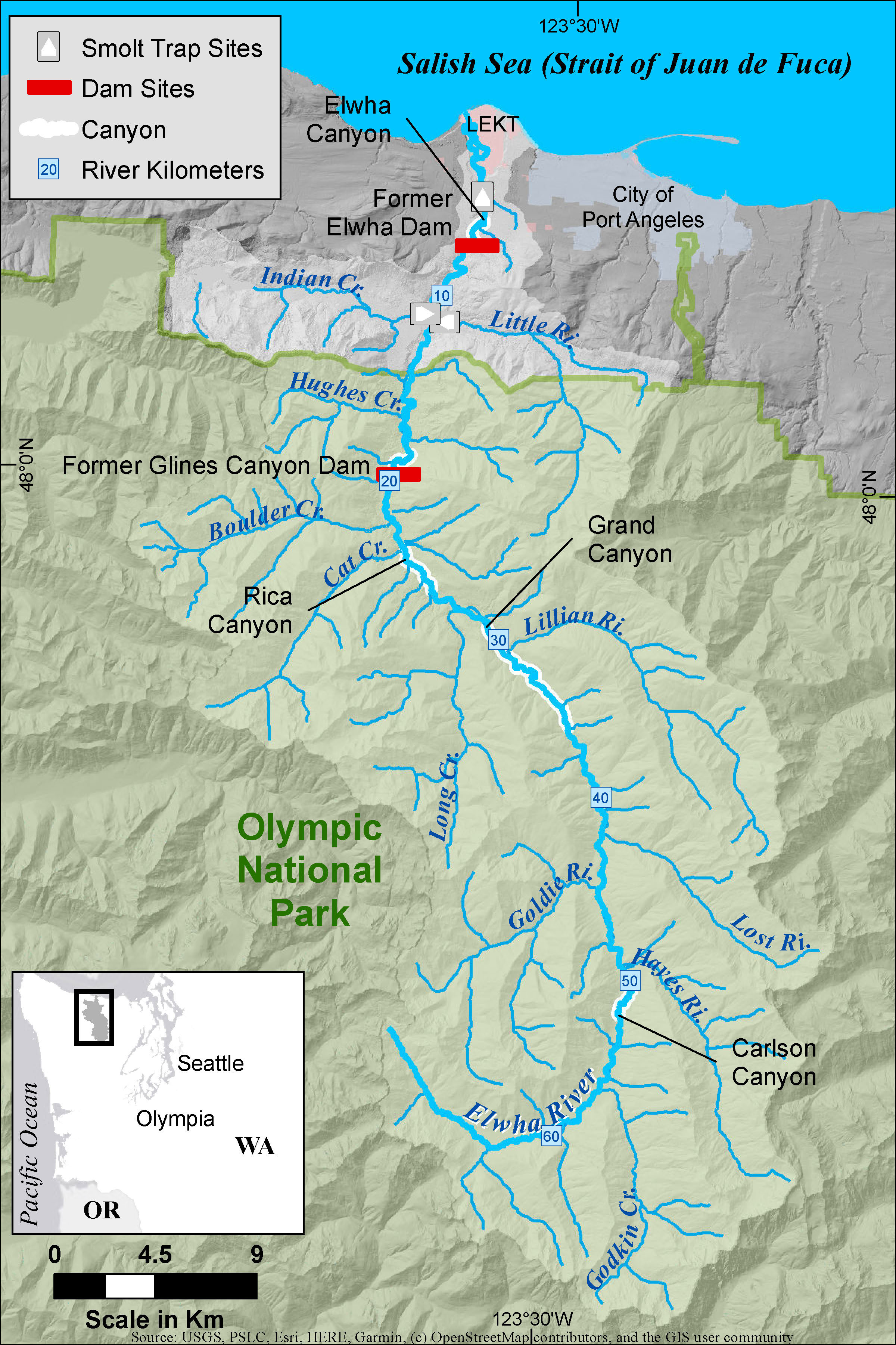
Figure 1 A map of the Elwha River with the locations of the three rotary screw traps, the former dams (red rectangles), and other features discussed in the manuscript. The Lower Elwha Klallam Tribal (LEKT) reservation is shown in pink.

We focused on two study tributaries which enter the Elwha River mainstem across from each other at rkm 12.9, Indian Creek from the west draining 62 $\text{k}{\text{m}}^2$, and Little River from the east draining 50 $\text{k}{\text{m}}^2$. Little River is relatively steep (mean gradient ~3.5%), cold (mean yearly water temperature ~7.5°C, Washington Department of Ecology, 2016), shaded, and snow melt dominated with headwaters originating at 1,615 m. Indian Creek is lower gradient (mean gradient < 1%), has a broad floodplain, is warmer (mean yearly water temperature ~9.0°C, Washington Department of Ecology, 2016), and is heavily influenced by its source, Lake Sutherland at an elevation of 155 m. We refer to locations in the mainstem and tributaries using rkm, which is defined here as the distance upstream from where the mainstem enters the ocean or from where the tributaries enter the mainstem.

2.2 Data

2.2.1 Smolt trap data

We used data from three rotary screw traps that captured juvenile fish as they migrated downstream (McHenry et al., 2023b). One trap was located in the mainstem river at rkm 4.0, a second in Little River at rkm 0.2, and a third in Indian Creek at rkm 0.6 (Figure 1) (McHenry et al., 2023b). The mainstem trap [2.44 m (8’) diameter] was located upstream of all hatcheries and downstream of the two tributaries. In both tributaries, smaller 1.22 m (4’) diameter traps were used. Traps were generally checked daily, and mark–recapture efficiency trials were conducted every 1 to 2 weeks at each trap. For each efficiency trial, a group of age zero (0+) fish were marked with a stain (Bismarck Brown) and released 500 m and 100 m above the mainstem and tributary traps, respectively. For the tributary traps, most fish used in the efficiency trials were 0+ Chinook or coho salmon captured in the traps. Recapture probabilities (efficiencies) averaged approximately 15% using releases averaging 100 fish. For the mainstem trials, hatchery 0+ Chinook salmon were used, with most release groups consisting of 1,000 fish. Mainstem efficiencies were considerably lower, averaging 3%. For all traps, the majority of the recaptured fish arrived within a few days of release. The total number of fish migrating past the trap was estimated by adjusting the catches using the period and trap-specific efficiencies (e.g., Carlson et al., 1998). Approximately once a week at each trap, lengths ( ± 1 mm) and weights ( ± 0.1 g) were measured for a subset of up to 20 Chinook salmon. All traps were installed in January or February and typically fished through July. Catch of juvenile Chinook salmon often started immediately upon installation of the trap, suggesting that a portion of the out-migration had already occurred. Catch of Chinook salmon out-migrants at the time of trap removal was typically negligible.

In this paper, we limit our analyses to age zero (0+) fish that comprise the majority of the fish captured in the traps. We identify potential age one fish (1+) by fitting a cubic smoothing spline (smooth.spline in R with 4 degrees of freedom) to the logged length versus date relationship for each year and trap independently, and then identifying points with model residuals greater than log(1.5). On the un-logged scale, this translates to lengths that were greater than 1.5 times the predicted median length at a given date. This rule was developed based on visual inspection of the data. When plotting fish lengths against time, we also identified groups of large fish captured in the tributary traps that we believed were hatchery fish used in the efficiency trials that stayed above the traps long enough to lose their marks. The Bismarck Brown stain usually begins to fade after a week and hatchery fish are generally larger than natural origin fish. After discussions with field biologists and determining the timing of efficiency trials in which hatchery fish were used, we identified potential anomalous lengths and excluded them. These included all lengths measured at the Indian Creek and Little River traps on 6 April 2022, and all Little River fish in 2021 with lengths greater than 45 mm before May 1. We used the models described below to further assess the validity of these assumptions (see Results). In total, less than 4% of the length data was excluded.

2.2.2 Redd survey data

To describe the spatial distribution of Chinook salmon spawning activity, redd (nest) surveys were conducted by foot each year during the predicted period of peak spawning (McHenry et al., 2023a). Redds were identified based on differences in the substrate coloration and stream bed morphology produced by the redd construction process and/or the presence of adults (Johnson et al., 2007). The redd surveys extended from the mouth of the Elwha River to rkm 63.4 (Figure 1), and included side channel and larger tributary habitat (McHenry et al., 2023a). Redd surveys in the two study tributaries, Little River and Indian Creek, extend from rkm 0 to rkm 1.9 (McHenry et al., 2023a), which included most of the observed spawning extent. For each year, we aggregated the redds by reach, where mainstem reaches were defined by rkm (e.g., rkm 1, rkm 2, …), and the tributary reaches included the entire survey reach (rkm 0–1.9) (Figure 2).

FIGURE 2

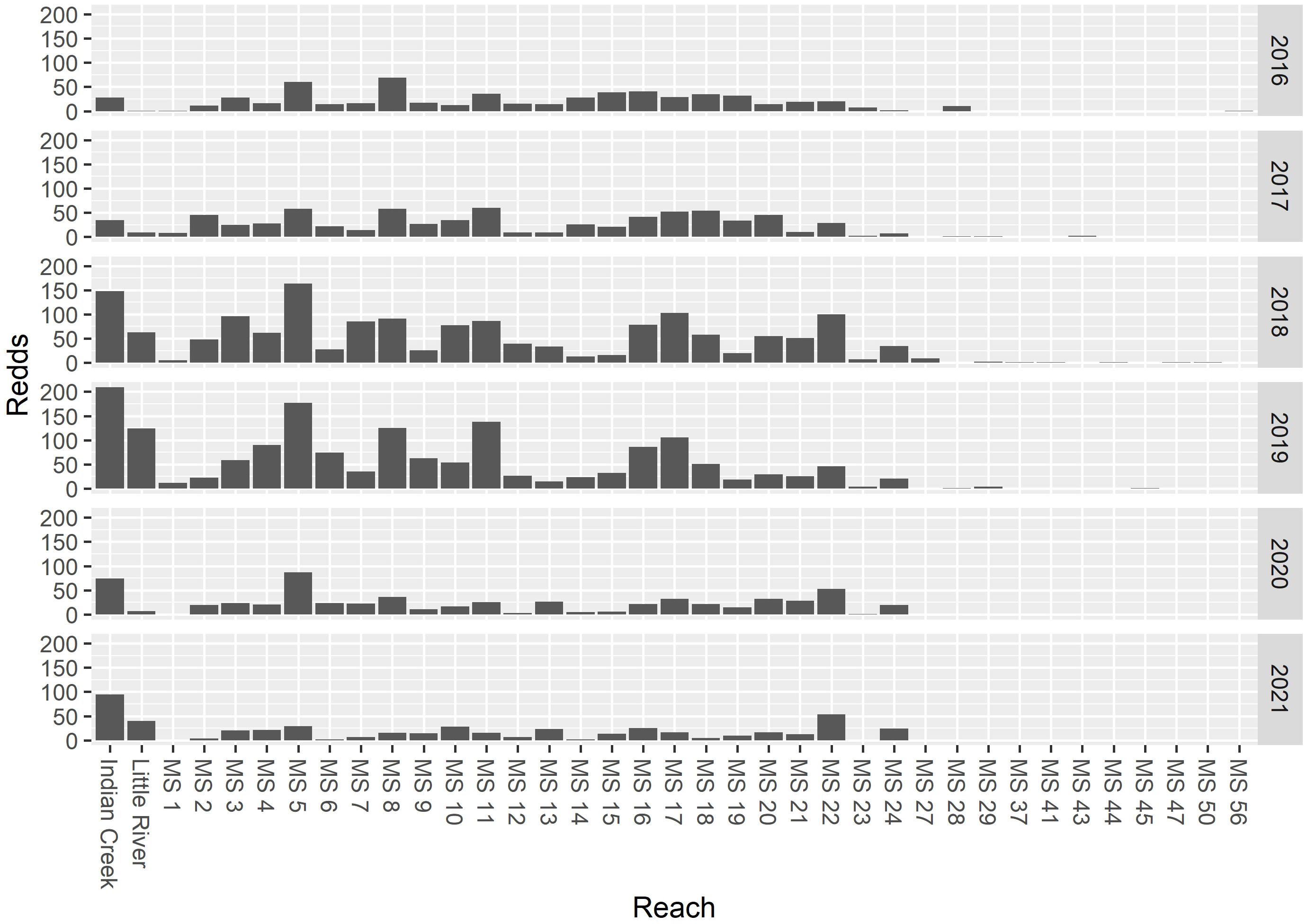
Figure 2 The total number of redds observed in 1-km mainstem reaches and in the two study tributaries, Indian Creek and Little River. The mainstem reach rkm X indicates the 1-km reach from river kilometer X−1 to river kilometer X.

The surveys were intended to describe spatial distribution (not abundance) and hence are timed to coincide with the peak of spawning based on historical averages and recent observations. Therefore, the spawn timing distribution is not captured in these surveys. However, spawning typically extends from the beginning of September to early to mid-October, peaking in mid- to late September (unpublished data).

2.2.3 Temperature data

During the study period (2018–2023), HOBO Water Temperature Pro v2 and TidbiT MX Temperature 400’ data loggers (± 0.2°C) (Onset Computer Corporation, Bourne, Massachusetts, USA) were deployed in the Elwha River basin to measure average daily water temperature at a number of locations. Loggers were set to record hourly and were cabled underwater to large wood. Loggers were encased in sun shields to protect from solar radiation and downloaded quarterly. The temperature loggers were located throughout the spawning range of Chinook salmon in the Elwha River, from rkm 2.5 to rkm 42.5 in the mainstem and at rkm 0.3 in Indian Creek and rkm 1.1 in Little River, respectively. Due to logistical issues, including the COVID pandemic, there were no loggers that were recording for the entire period and there were periods when no loggers were recording. For this study, we used the available logger data and data from a site on the Quinault River (also on the Olympic Peninsula) to build a model that predicted mainstem water temperature within the spawning range based on date (between 2018 and 2023) and rkm. In addition, we filled in water temperature data in the sites in the two study tributaries (Little River and Indian Creek), using a model describing the seasonal temperature relationship between the two tributaries and a mainstem site. See Supplementary material Appendix A for details of how the temperature series were constructed.

2.2.4 Emergence size

The size at emergence of juvenile Chinook salmon varies considerably between and within redds, and between populations (Beacham and Murray, 1990). While we do not have direct estimates of size at emergence for Elwha River fish, we can infer size based on the observed distribution of egg weights and the estimated relationship between egg weight, temperature, and emergence size reported in Beacham and Murray (1990, Equation 11). Using an average egg weight, 246 mg, and standard deviation, 37 mg, based on measurements from 205 Chinook salmon examined at the WDFW Elwha River hatchery facility between 2015 and 2021 (unpublished data), a predicted average fry length of 35.9 mm was produced, for an average incubation temperature of 7°C. Predicted fry length changed slightly with changes in incubation temperatures, with 5, 6, 7, 8, and 9°C producing lengths of 35.7, 36, 35.9, 35.8, and 35.5 mm, respectively. Egg weight had a larger impact. Adding and subtracting one standard deviation from the mean egg weight, with an incubation temperature of 7°C, produced lengths of 35.1 and 36.7 mm. For the primary analysis, we used an emergence length of 36 mm but we explored the sensitivity of the results to this assumption in Supplementary material Appendix B. Emergence lengths in other studies were comparable to this value (e.g., Murray and Beacham, 1987; Geist et al., 2010).

2.3 Models

For each trap–year combination (12 in total), we sequentially applied the spawn timing model, emergence model, and growth model to produce estimates of emergence timing and juvenile length at date for different years and locations in the watershed. We then combined these models with the movement model to predict the timing and lengths of juveniles captured in the three rotary screw traps (Figure 3). Comparing these aggregate model predictions to the observed timing and lengths allowed us to identify potential problems with the model assumptions and describe combinations of spawn timing and movement model parameter values that best predicted the observations. Parameters for each sub-model are described in Table 1. We attempted to keep the models simple enough to use for inference, while allowing sufficient complexity to explain important biological and demographic processes. We acknowledge that there are many plausible explanations for the observed patterns, only some of which are accommodated by the models we used. We explored the sensitivity of our results to additional changes in the model form in Supplementary material Appendix B. For the incubation and growth models, we adopted the parameter and variable naming conventions used in the manuscripts where the models were developed.

FIGURE 3

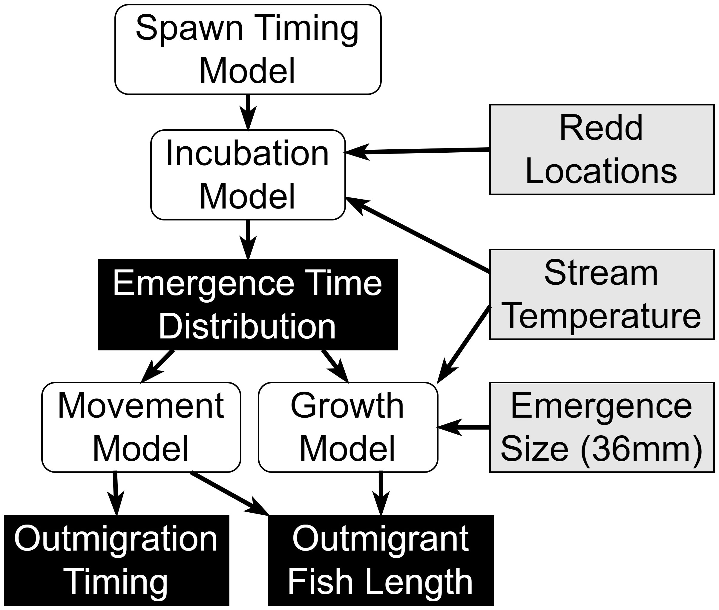
Figure 3 A diagram illustrating the different model components (white), input assumptions and data (gray), and model predictions (black).

TABLE 1

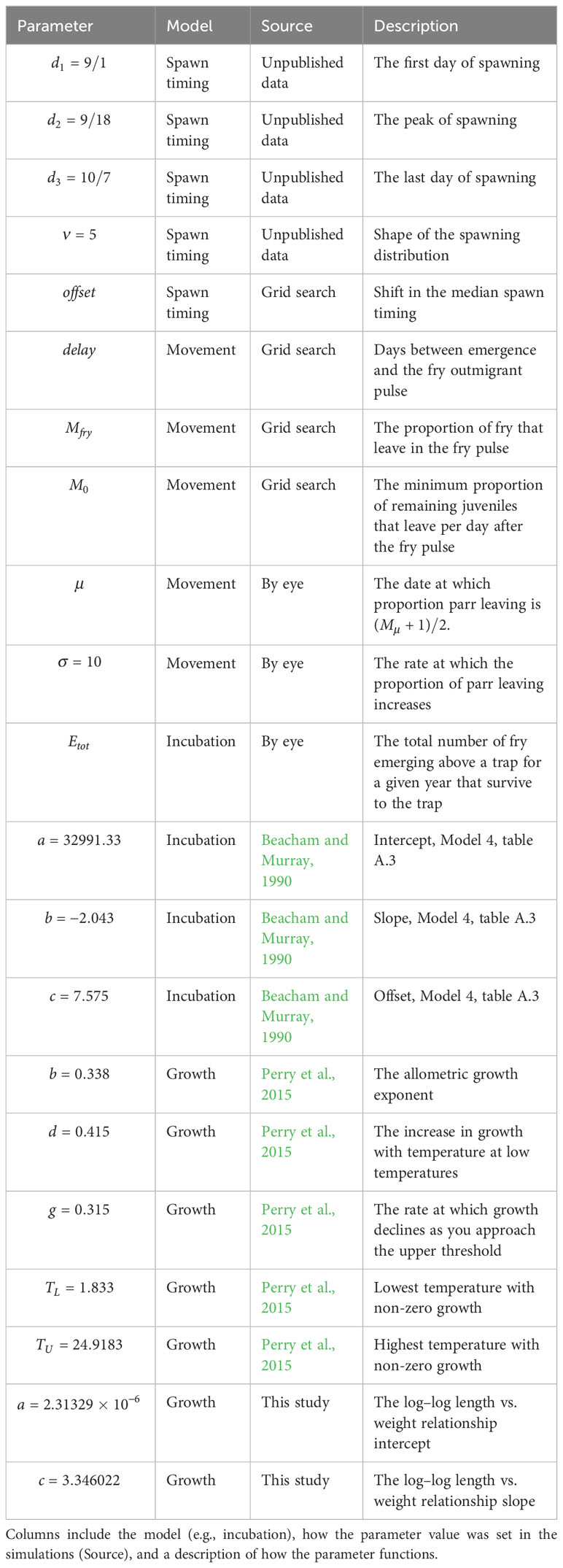
Table 1 Description of the model parameters.

2.3.1 Spawn timing

The spawn time distribution was assumed to follow a generalized beta distribution starting on September 1, peaking on September 18, and ending on October 7 (Figure 4A; see Supplementary material Appendix C). These dates are based on observations by biologists familiar with the river and represent an average timing across multiple years (unpublished data). To accommodate differences in spawn timing between years and across locations, we included an offset parameter, $offset$, that shifted the distribution earlier or later in time by up to 14 days.

FIGURE 4

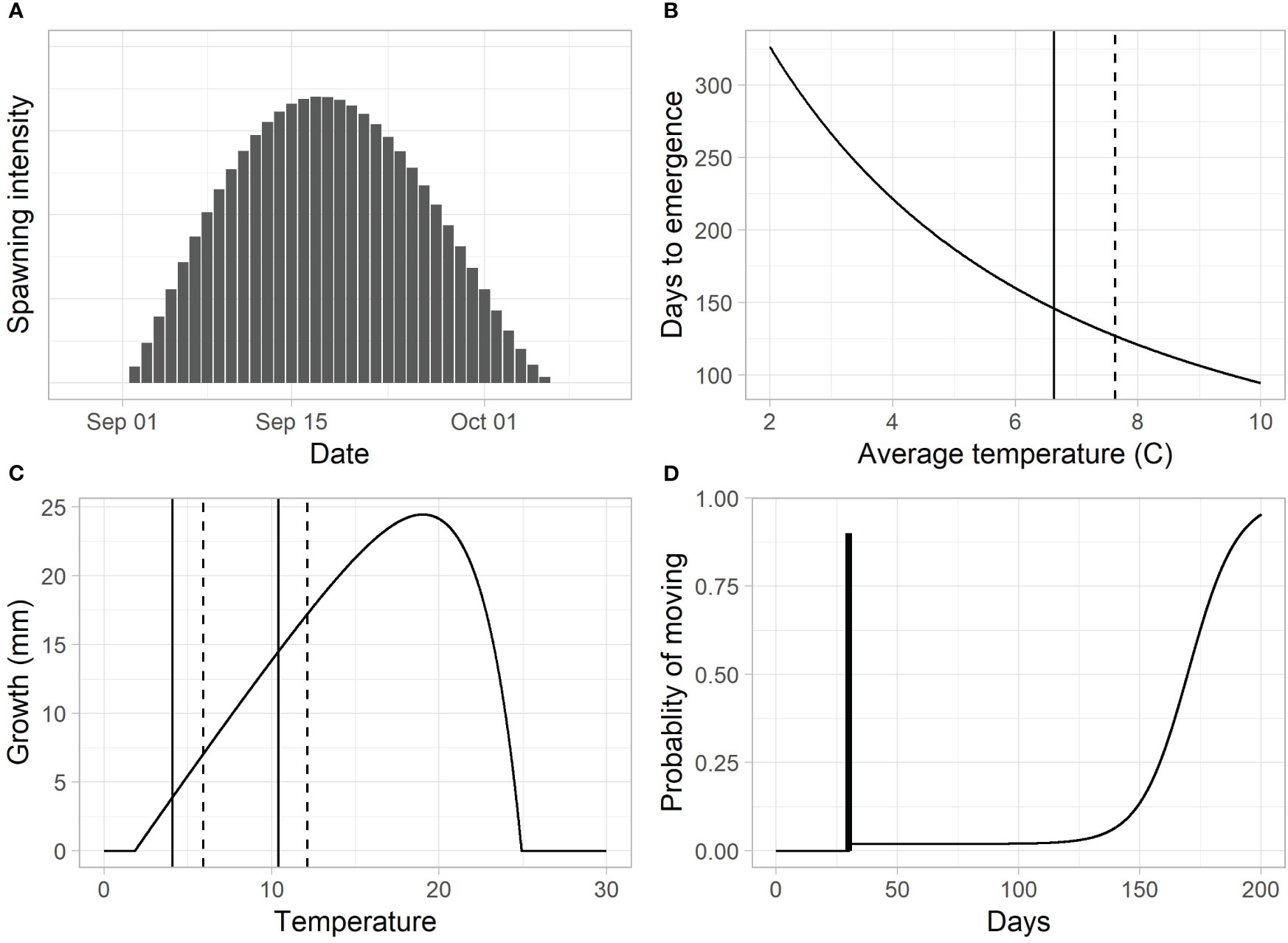
Figure 4 (A) The assumed spawn time distribution based on the generalized beta function. (B) Predicted emergence times for different average incubation temperatures (vertical lines = average incubation temperatures for the mainstem, solid, and Indian Creek, dashed). (C) Growth for a 40-mm fish over a 28-day period (vertical lines represent average temperatures in February and June for the mainstem, solid, and Indian Creek, dashed). (D) The proportion of fish above the trap that move past the trap per day. In this example, the dark vertical bar represents the pulse of fry (90%) leaving 30 days after emergence. The increasing function after day 30 represent the parr migration, with a rapid increase in out-migration at approximately day 150.

2.3.2 Incubation

The length of the egg incubation period, $D$, was modeled using a model described in Beacham and Murray (1990, model 4) (Figure 4B).

$$loɡ\left(D\right)=loɡ\left(a\right)+b\times loɡ\left(T-c\right)$$

where $T$ is the average temperature during the incubation period. The parameters $a$, $b$, and $c$ are estimated in Beacham and Murray (1990, Table 1). Because fish from an individual redd emerge over multiple days, we used a normal distribution centered on the predicted emergence date with standard deviation two, to spread the emerged fry across multiple days (e.g., Field-Dodgson, 1988). For the mainstem trap, with a diverse set of upstream temperature regimes, we divided the river into reaches (Figure 2), used reach specific temperatures to calculate the emergence times for redds from each reach and year, and combined the emergence times into a single aggregate emergence time distribution for each year, weighting by the relative number of redds in each reach. For each of the tributaries, we modeled incubation using a single temperature series since the spawning extent was relatively compact (rkm 0 to rkm 1.9). The end product for each year and trap was the proportion of total fish, $P_t$, that emerged on each day, $t$.

2.3.3 Growth

We used a length-based version of a juvenile Chinook salmon growth model, $f_{ɡ}$, developed by Perry et al. (2015), which predicts length, $L_t$, at day $t$ based on an initial length at day 0, $L_0$, and the average temperature during the growth period, $T$ (Figure 4C, see Supplementary material Appendix C for model details),

$$L_t=f_{ɡ}\left(L_0,t,T\right)={\left(L_0^{cb}+d\left(T-T_L\right)(1-e^{ɡ(T-T_U)})\frac{bt}{a^{b}100}\right)}^{\frac{1}{cb}}$$

The model parameters $T_L$ and $T_U$ (the minimum and maximum temperatures at which growth is positive), $d$ and $g$ (rate parameters), and $b$ (an allometric growth exponent) were all estimated in Perry et al. (2015) (Table 1). The parameters $a$ and $c$ define the log–log relationship between lengths and weights and were estimated in this study based on captured fish measured at the three traps during the study period (Table 1). For the tributaries, we used the same temperature series that was used in the incubation model, while for the mainstem, we used temperatures for rkm 13, which is near the center of the redd distribution post dam removal, in an attempt to describe average conditions during migration to the trap.

2.3.4 Combined model with movement

To translate the predicted emergence times and growth trajectories into estimated out-migrant timing and size at the smolt trap, we modeled stream residence and migration past the trap. Juvenile movement is a complex process occurring across space and time. Here, we simplified the process to movement from above to below the smolt trap, combining all fish that emerged on a specific day above the trap into a single group.

The number of fish that emerged on day $t_e$ was modeled as the predicted proportion of fish that emerged on that day, $P_{t_e}$ (from the incubation model), times the total number of fish that emerged that season, $E_{tot}$ (a model parameter).

$$N_{t_e,t_e}=E_{tot}{P}_{t_e}$$

Here, the first index on $N$ indicates the emergence day for this group. Thus, $N_{t_e,t}$ represents the number of fish that emerged on day $t_e$ that are above the trap on day $t$, where $t\ge t_e$. Day $t$ represents Julian date (i.e., days since January 1 of the given trap year + 1). The value of $N_{t_e,t}$ was updated each day until the end of summer to reflect downstream migration past the trap,

$$N_{t_e,t}=N_{t_e,t-1}\left(1-m_{t-t_e,t}\right)$$

where the rate of movement past the trap, $m_{a,t}$, on day $t$ is a function of the days since emergence, $a=t-t_e$, and the current day, $t$. Fish moving past the trap were therefore:

$$O_{t_e,t}=N_{t_e,t-1}{m}_{t-t_e,t}$$

The movement model assumed a fraction, $M_{fry}$, of the fish left as a pulse at a specified number of days, $a=delay$, after emergence. Probability of movement after the pulse was assumed to be a function of day, $t$, starting at a baseline migration rate of at least $M_0$ and increasing to 1 with a logistic form (Figure 4D).

$$m_{a,t}=\{\begin{array}{cc}0& \text{if }a\le delay\\ M_{fry}& \text{if }a=delay+1\\ M_0+\left(1-M_0\right){\left(1+e^{\left(t-\mu \right)/\sigma }\right)}^{-1}& \text{if }a>delay+1\end{array}$$

Here, $\mu$ regulated the timing of the increase in parr migration rate, and $\sigma$ controlled how quickly the rate increased (Figure 4D).

Because simultaneously estimating mortality and the total number of fish that emerged would be difficult with these data, we modeled fish that would eventually survive to move past the trap.

Length for the group corresponding to each emergence day, $t_e$, was initialized at 36 mm ($L_{t_e,t_e}=36$) and then updated daily thereafter using the growth model (see above), the temperature on that day, $T_t$, the length on the previous day, $L_{t_e,t-1}$, and a growth period of 1 day.

$$L_{t_e,t}=f_{ɡ}\left(L_{t_e,t-1},1,T_t\right)$$

To create summaries that could be compared to the daily numbers and lengths of out-migrants observed at the traps, we summed across emergence day to get total out-migrants for each day $t$.

$$O_t={\displaystyle \sum _{t_e=d1}^{d2}{O}_{t_e,t}}$$

Here, $d1$ and $d2$ are the first and last days that fish emerged for the given trap and year. We calculated the median predicted length of fish on each day.

$$L_t=median\left(rep\left(L_{·,t},O_{·,t}\right)\right)$$

Here, $rep\left(L_{·,t},O_{·,t}\right)$, is a vector with lengths for each of the $O_t$ out-migrants on day $t$, where the length for fish that emerged on day $t_e$ was replicated $O_{t_e,t}$ times. The vectors $L_{·,t}$ and $O_{·,t}$ represent all of the lengths or out-migrants for the different emergence days, predicted on day $t$.

2.4 Model evaluation

Because the models were deterministic and ignored many complexities of early life history, we used simple metrics to describe how well the predicted timing and sizes captured the observed values. For example, out-migration timing tends to occur in pulses regulated by factors such as patchy timing of redd construction, river discharge, and other physical habitat factors. Instead of trying to capture those pulses, we described more general characteristics that are less sensitive to small-scale patterns. While the simulation model produced a daily distribution of out-migrant lengths, we made no effort to realistically represent this variability and therefore focused on metrics based on the median predicted out-migrant length at each day. See Supplementary material Appendix C for further discussion about the model evaluation approach and method of parameter space exploration.

2.4.1 Model fit

We used four metrics to evaluate model agreement with the data. The first compared the predicted and observed date of transition from fry to parr migrants, the second and third compared predicted to observed fry and parr migrant lengths, and the final metric compared the observed and predicted proportion of out-migrants leaving between trap installation and the transition from fry to parr migrants. We focused only on the relative out-migrant timing (i.e., the shape of the curve) ignoring comparisons between total numbers of observed and predicted out-migrants.

Fry-to-Parr Transition (Δf2p): Ocean-type juvenile Chinook salmon tend to migrate downstream as fry soon after emergence or rear in the river for a few additional weeks or months before migrating as parr in late spring or summer (e.g., Zimmerman et al., 2015; Anderson and Topping, 2018). For the Elwha River trap–year combinations covered in this manuscript, the fry migrants outnumber the parr by at least 10 to 1, resulting in a sudden drop in out-migrants at the end of the fry migration. We use the number of days between the observed and predicted date of this transition as a measure of fit (Δf2p). The date of this transition, f2p, was estimated by smoothing the daily out-migrant series with a 7-day moving average and then finding the first date at which the smoothed series fell below 5% of the previous maximum value. Notice that using observed lengths to identify this transition was not possible due to large temporal gaps in the length data for some trap–year combinations.

$$\Delta f2p=\left|f2p_{pred}-f2p_{obs}\right|$$

Fry and Parr Length (ΔlenF, ΔlenP): We subtracted the log of the observed and predicted lengths of each measured fish during the fry migration period and parr migration period. The fry and parr migration periods were defined using the fry-to-parr transition calculated for the observed data, $f2p_{obs}$. The predicted out-migrant length for a specific day is defined as the median of the predicted sizes (see above). We took the mean of these differences to calculate the bias, and then took the absolute value of the bias, exponentiated the result, and subtracted this value from one to get a metric on the original scale. This meant that the bias was multiplicative. Therefore, predictions that were on average x times the observations would produce the same result as observations that were on average x times the predictions.

$$\Delta lenF=1-exp\left(\left|{\displaystyle \sum _{i=1}^{N_{fry}}\left(log\left(L_{t\left[i\right]}\right)-log\left(L_{obs,i}\right)\right)/N_{fry}}\right|\right)$$

$$\Delta lenF=1-exp\left(\left|{\displaystyle \sum _{i=1}^{N_{fry}}\left(log\left(L_{t\left[i\right]}\right)-log\left(L_{obs,i}\right)\right)/N_{parr}}\right|\right)$$

Here, $L_{t\left[i\right]}$ is the predicted median length on day $t\left[i\right]$ where $t\left[i\right]$ is the day of the $i^{th}$ observed fry or parr length, $N_{fry}$ and $N_{parr}$ are the total number of observed fry and parr lengths, respectively, and $L_{obs,i}$ is the $i^{th}$ observed fry or parr length.

Percent fry migrants (ΔpFry): For both the observed and predicted out-migrants, we calculated the proportion of juveniles that migrated past the trap between the installation of the trap and the transition from fry to parr migrants, pFry. We used the observed date of transition from fry to parr as described in the fry-to-parr transition metric above ($f2p_{obs}$). The fit metric was defined as the absolute value of the difference between the observed and predicted metrics.

$$\Delta pFry=\left|pFr{y}_{pred}-pFr{y}_{obs}\right|$$

2.4.2 Plausible parameter combinations

We defined plausible fits as those parameter combinations for which the differences between the observed and predicted values were less than parameter-specific tolerances. Specifically, a set of parameters was defined as plausible when the difference in fry-to-parr transition between the observed and predicted data, Δf2p, was less than 4 days, the absolute length bias for both fry and parr, ΔlenF and ΔlenP, was less than 10% (0.1), and the difference between the proportion of observed and predicted fry migrants, ΔpFry, was less than 2% (0.02). These criteria were derived by looking at fits and making a subjective decision about which fits appeared believable. We highlighted a specific parameter combination for plotting by minimizing the following objective function:

$$\frac{\Delta f2p}{4}+\frac{\Delta lenF}{0.1}+\frac{\Delta lenP}{0.1}+\frac{\Delta pFry}{0.02}+max\left(1,\frac{\Delta f2p}{4}\right)+max\left(1,\frac{\Delta lenF}{0.1}\right)+max\left(1,\frac{\Delta lenP}{0.1}\right)+max\left(1,\frac{\Delta pFry}{0.02}\right)$$

The last four terms of the expression penalize parameter values outside of the plausible parameter ranges (i.e., they are 1 within the plausible range and >1 outside of the plausible range).

2.4.3 Parameter exploration

The parameters for the emergence and growth models were taken from the respective papers and assumed fixed (Table 1). We used a grid search to explore possible parameter combinations for the spawn timing offset and movement model parameters primarily responsible for patterns captured in the fit metrics described above ($offset$, $delay$, $M_{fry}$, $M_0$). For each of these parameters, we chose a set (size = n) of values that spans a biologically reasonable range, and then examined all possible combinations of these values for the different parameters. The grid search parameters included the number of days between emergence and fry out-migration, $delay$ (0 to 30, n = 31), the adjustment to median spawn timing, $offset$ (−14 to 14, n = 29), the initial rate of parr migration, $M_0$ (0.001 to 0.01, n = 11), and the proportion of out-migrants that leave as fry, $M_{fry}$ (0.905 to 0.995, n = 10). For all sets, we used equal steps except for $M_0$ where we used equal steps on the log scale (${10}^{-\left(2 to3by0.1\right)}$). The total number of parameter combinations was $31\times 29\times 11\times 10=98,890$, which was repeated for the 12 different trap–year combinations. The date at which parr migration increases in the summer, $\mu$, and the total number of out-migrants, $E_{tot}$, were determined through trial and error using graphical comparisons of the observed and predicted out-migrants for each trap–year combination. The rate at which the parr migration increased, $\sigma$, was set to 10 for all trap–year combinations again based on graphical analysis. Because the fit metrics focus on the transition from fry to parr migrants and lengths, they were not as sensitive to these three parameters. For each trap–year combination, fits based on all parameter combinations were determined to be plausible or not plausible based on the criteria above, and the combination with the lowest value of the objective function described above was used to identify a single parameter combination for plotting. To explore the sensitivity of the results to different emergence sizes and growth rates, we repeated the analysis for three additional scenarios in Supplementary material Appendix B.

3 Results

3.1 Temperatures

Stream temperatures differed between years and reaches (Figure 5). Relative to the mainstem (rkm 13), temperatures in Indian Creek were 1 to 2°C warmer in the winter and 1 to 2°C cooler in the summer, with temperatures increasing earlier in the spring. Little River had similar temperatures to the mainstem in the winter, but was cooler in the summer by 1 to 3°C.

FIGURE 5

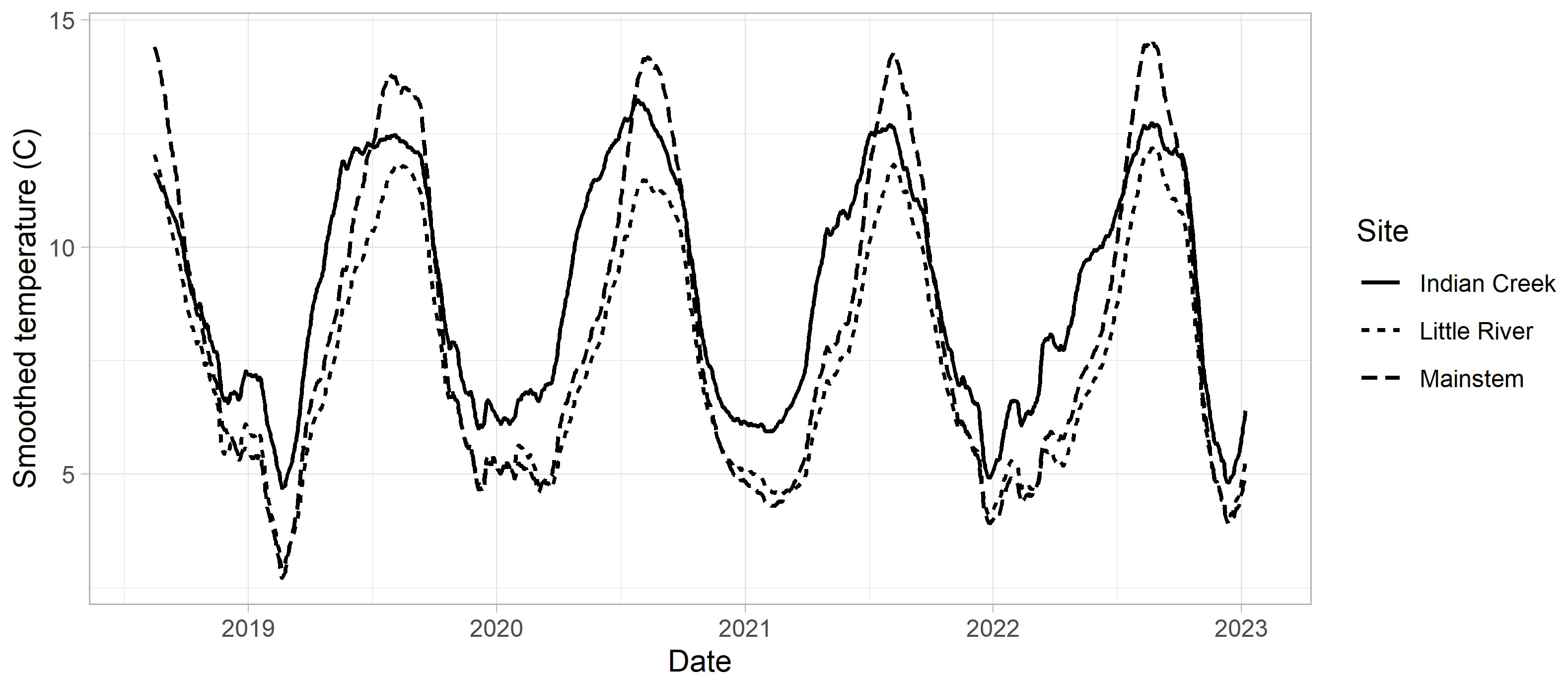
Figure 5 Temperature data for Indian Creek, Little River, and the mainstem site adjacent to the USGS gage (rkm 13, near the center of the redd distribution post dam removal). A 31-day moving average was applied to all series to improve visualization. See Supplementary material Appendix A for details of how these temperature series were prepared.

3.2 Emergence timing

Predicted emergence time varied by habitat type (mainstem vs. tributaries), reach, and year when the spawn time distribution was held constant (Figure 6A). Warmer stream temperatures in lower Indian Creek during incubation led to predicted emergence times that were approximately a month earlier than in Little River for the same spawn timing (Figure 7). There were similar differences between sites in the lower Elwha (rkm 2) and upper Elwha (rkm 42) mainstem sites. The predicted aggregate emergence time distribution for the Elwha mainstem, weighting by Chinook salmon redds per reach, fell in between Indian Creek and Little River distributions and tended to be more protracted relative to the tributaries or individual mainstem reaches. There were also predicted differences in emergence timing by year, with median emergence for the 2021 spawners (2022 out-migrants) predicted to occur close to a half of a month later than for the 2018 spawners (2019 out-migrants) (Figure 6A). Water temperature tends to decrease during the incubation period, which meant that eggs from redds constructed earlier were predicted to develop faster. This resulted in emergence time distributions that were broader than the spawn timing distributions (Figure 7).

FIGURE 6

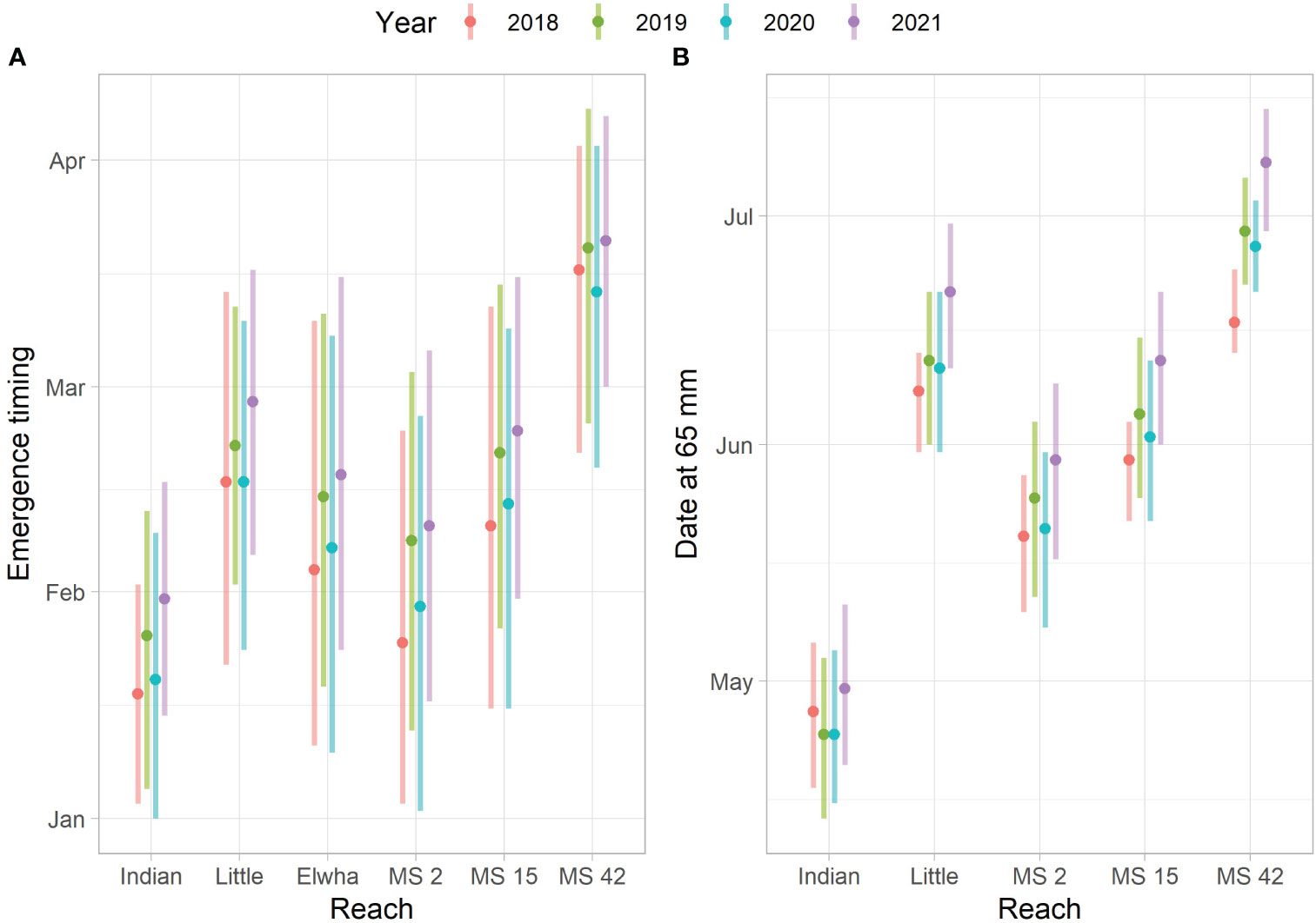
Figure 6 Predicted emergence timing and date at which fish have grown to 65 mm. (A) The 10th, 50th, and 90th quantiles for the predicted emergence time distributions for each reach and year. The Indian Creek (Indian) and Little River (Little) reaches represent the lower 1.9 km where most spawning occurs. The Elwha reach refers to the aggregate predicted emergence based on reach and year-specific temperature series and redd numbers. MS 2, MS 15, and MS 42 indicate mainstem reaches at rkm 2, rkm 15, and rkm 42 respectively. (B) The predicted dates at which fish have grown to 65 mm for fish emerging on the 10th, 50th, and 90th date quantiles (see left panel).

FIGURE 7

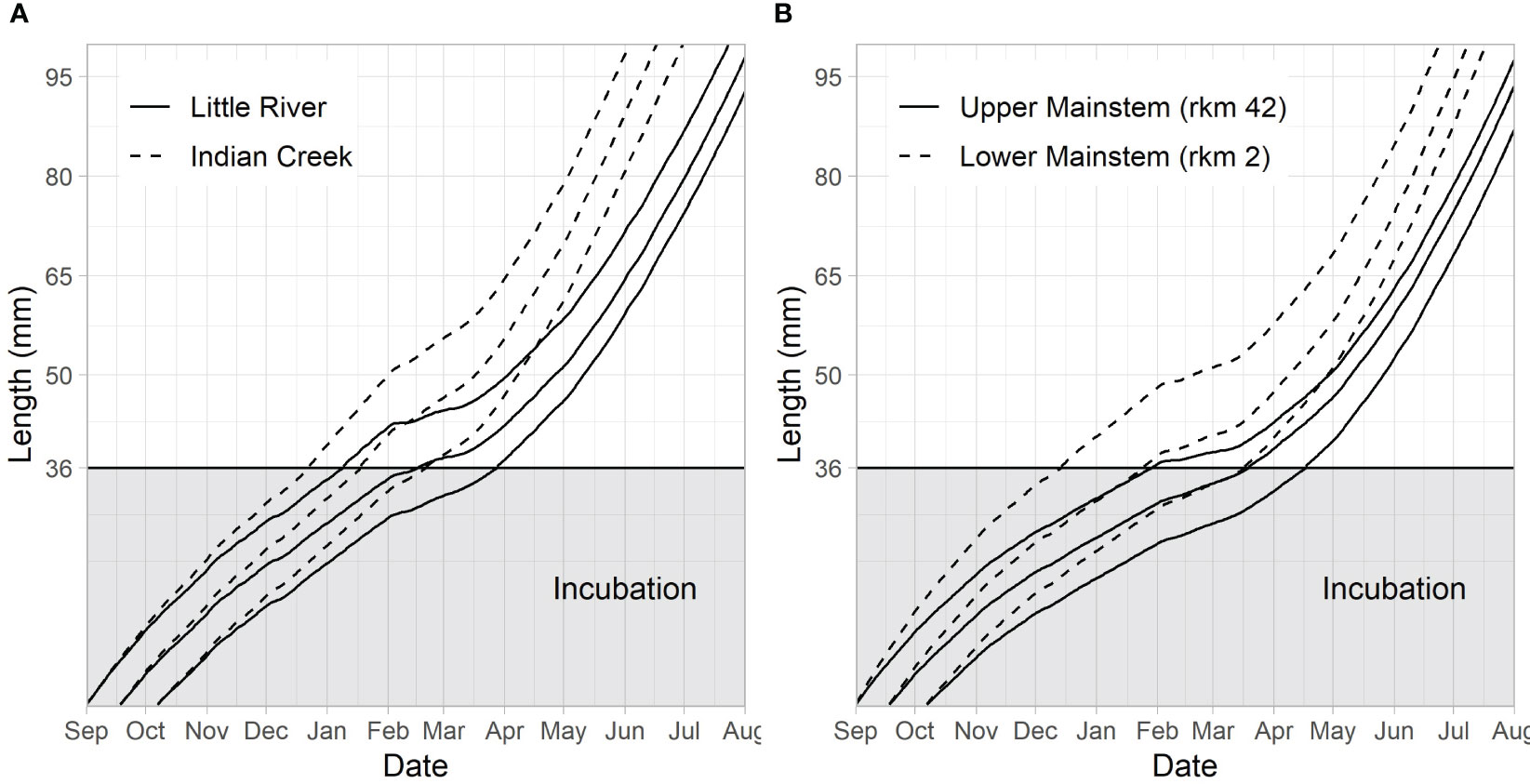
Figure 7 Embryo development and juvenile fish growth in 2018 from redds at the beginning (Sept 1), middle (Sept 18), and end (Oct 7) of the assumed spawn time distribution. The y-axis during incubation is the percent development of the embryo, with 100% development coinciding with a size of 36 mm (the assumed emergence size). Percent development at time t is defined as (degree days at time t)/(degree days at emergence)×100. (A) Compares trajectories for the two tributaries, Little River and Indian Creek. (B) Compares trajectories for a reach in the lower river (rkm 2) and a reach in the upper river (rkm 42).

3.3 Growth

Emerging Chinook salmon fry were predicted to experience different stream temperatures due to differences in emergence time and location. This led to differences in predicted growth rates (Figure 7). Differences in the date at which juvenile Chinook salmon were predicted to reach 65 mm were similar to differences identified in predicted emergence timing, although increasing temperatures after emergence tended to result in narrower date ranges at which fish reach 65 mm (when compared to emergence dates) because earlier emerging fish grow slower and later emerging fish grow faster (Figures 6, 7). Predicted differences between Indian Creek and Little River were pronounced, with most Indian Creek juvenile Chinook salmon predicted to achieve 65 mm by the beginning of May while Little River juvenile Chinook salmon were predicted to reach this size primarily in June (Figures 6B, 7A).

3.4 Full model predictions

When the movement model was added to the spawn timing, incubation, and growth models, the combined model was able to explain the observed fish lengths and the timing of the fry-to-parr transition for most trap–year combinations (Figure 8; Table 2). Specifically, the grid search produced plausible parameter combinations for all but 2 years in Indian Creek (Figure 9). In most cases, there were many plausible parameter combinations. In fact, for 8 of the 12 trap–year combinations, the range of plausible $delay$ values was more than 20 days (Figure 9). As the $delay$ parameter increased, the plausible spawn timing shifted earlier (i.e., smaller $offset$) in order to explain the same out-migrant timing. For example, the observed timing and lengths of 2019 Little River out-migrants could be explained by a late spawn timing (offset = 14) and immediate fry out-migration (delay = 0) or early spawn timing (offset = −5) and a delayed fry out-migration (delay = 30). For some trap–year combinations, the fit to the length data also constrained the plausible set. For example, in 2022, the mainstem and Little River parr lengths could only be explained with earlier spawning and a longer delay between emergence and fry out-migration. In Indian Creek, there were only 2 years in which the grid search produced parameter combinations that satisfied the parr length criteria (2019 and 2021). However, if the growth rate was reduced by 25% to reflect food limited growth, there were plausible fits for all years (Supplementary material Appendix B). Even though there were often many plausible parameter combinations, there were some consistent patterns in the plausible sets across traps. For example, if delay was assumed to be constant across years, then the plausible spawn timings were later for juveniles in 2020 and earlier for those in 2022 for all traps. The decision to exclude some fish lengths that were inconsistent with the other length data (orange points in Figure 8) was supported by the model results. In almost all cases, the excluded points were far from the predicted lengths. For some trap–year combinations, it appeared that the trap was installed after significant numbers of fry had migrated past the trap (e.g., Little River 2020, Indian Creek 2021, and mainstem 2019 Figure 8). For trap–year combinations where it appeared that the traps were installed before substantial out-migration, the predicted and observed timing of out-migration initiation was not always consistent. In particular, in some years, it appeared that the observed initiation of out-migration occurred as much as a month after the predicted initiation (e.g., Little River 2019 and Indian Creek 2022, Figure 8). While we did not focus on timing of the parr out-migration, using a single hand fit value for the parameter defining the end of parr migration, $\mu$, the model approximately captures the shape of the parr migration for the different trap–year combinations (Figure 1 in Supplementary material Appendix D).

FIGURE 8

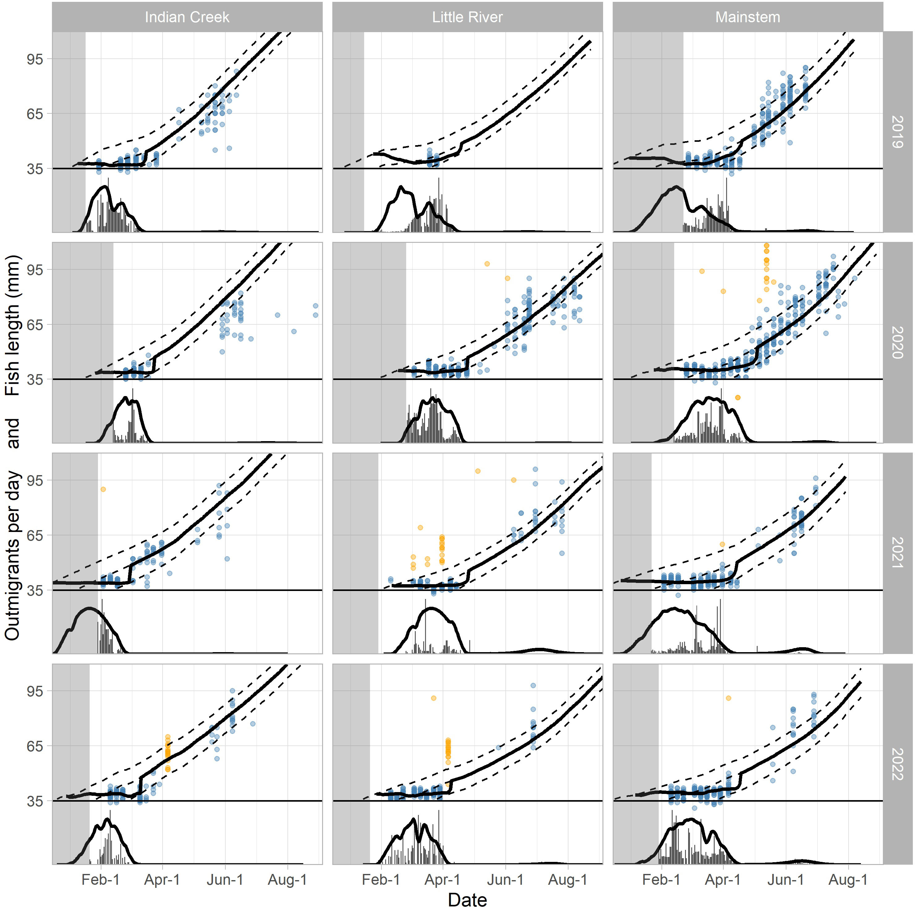
Figure 8 Observed and predicted out-migrant timing and lengths for the three traps and 4 years. Out-migrant timing is plotted below the solid horizontal line at y = 35, and the y-axis represents the daily number of out-migrants scaled by year and trap to fit within the available space. Out-migrant lengths are plotted above the solid line at y = 35 and the y-axis represents out-migrant length in mm. For both out-migrant timing and lengths, the thick black lines are the predictions corresponding to the best fit (black points in Figure 9). The dashed lines above y = 35 are the growth trajectories for fish emerging at the start, middle, and end of the predicted emergence time distribution corresponding to the best fit. The observed number of daily out-migrants is plotted as gray vertical bars (below y = 35) and the observed lengths for individual fish captured and measured in the traps are represented by points (above y = 35). The orange points are lengths that were not included when calculating the fit statistics due to discrepancies with the other length data (see Materials and Methods). The light gray region delineates the period before the trap was installed.

TABLE 2

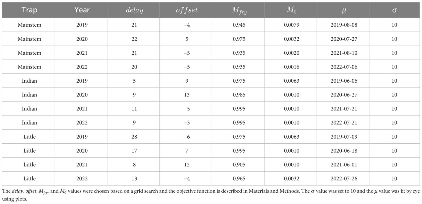
Table 2 The best-fit parameter combinations used for plotting the predictions in Figure 8.

FIGURE 9

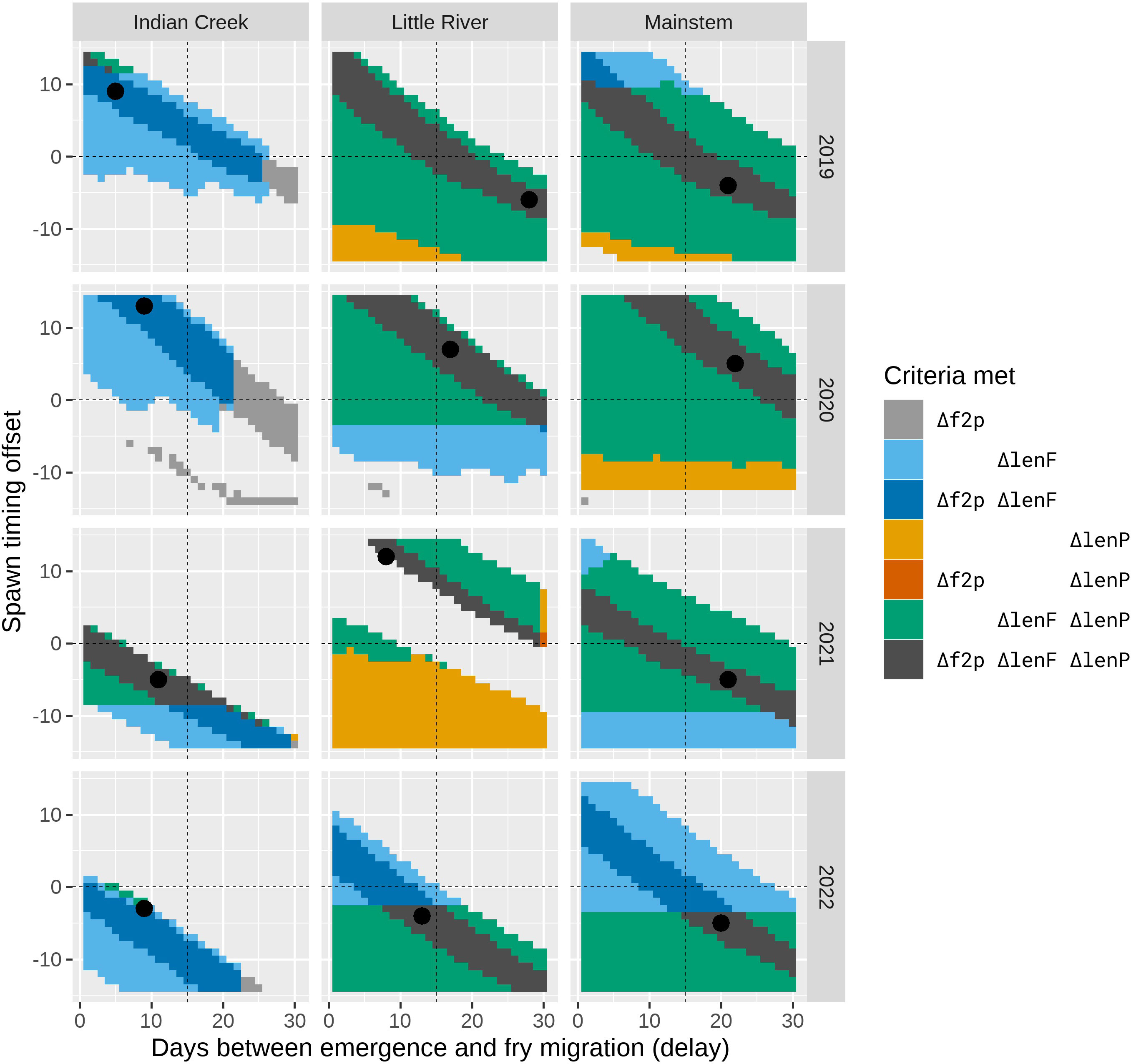
Figure 9 The combinations of the delay and offset parameters that resulted in plausible fits to the observed data as defined by the different fit criteria. The shaded areas represent combinations of the delay and offset parameters where at least one of the fit criteria Δf2p, ΔlenF, or ΔlenP was met and the criterion ΔpFry was also met. The dark gray area indicates that all criteria were met (i.e., plausible fits), and the black point identifies the parameter combination corresponding to the best fit as defined by the objective function in Materials and Methods. Other colors indicate parameter pairs where different combinations of the fit criteria were achieved (see the legend).

4 Discussion

The removal of two dams in the Elwha River increased the diversity of stream temperature regimes available to Chinook salmon (Figure 5), resulting in increased variability in predicted emergence timing and growth trajectories (Figures 6, 7). Predicted median emergence times and the date at which juveniles reached 65 mm differed by up to 2 months across locations within the watershed. We postulate that this diversity of emergence times and growth trajectories increases the chances that there will be juveniles that are well suited to year-specific conditions, resulting in higher population resiliency when compared to the pre-dam conditions (Greene et al., 2009; Schindler et al., 2010; Thorson et al., 2014).

This increased diversity of emergence times and growth trajectories may also result in the expansion of life history strategies that spend more time in the river rearing before ocean entry. Currently, there are very few natural origin juvenile Chinook salmon rearing above the traps past the fry stage, with fry comprising over 95% of out-migrants in most years (McHenry et al., 2023b) (Figure 8). The stream-type life history, where juveniles enter the ocean at age 1, is linked to colder rearing temperatures (Beckman and Dickhoff, 1998; Beechie et al., 2006) and may become more prevalent as spawning continues to expand into the upper watershed, characterized by colder temperatures. In addition, variable emergence timing and growth rates may provide more efficient utilization of the available rearing habitat through sequential use and size specific habitat preferences (Everest and Chapman, 1972). Attaining a larger size before leaving the river may be particularly important for population recovery in the Elwha River where estuary habitat is limited relative to other Puget Sound rivers reducing opportunities for growth before ocean entry. Campbell and Claiborne (2017), for example, found that in Puget Sound watersheds with little available intact estuary habitat, very few returning adult Chinook salmon had adopted the fry migrant strategy as juveniles, suggesting low marine survival of this life history strategy.

When the individual models were combined to predict out-migrant timing and lengths at the three screw traps, we found parameter combinations that satisfied all fit criteria for 10 of the 12 trap–year combinations (Figures 8, 9). While there were many plausible combinations of the $delay$ and $offset$ parameters for most trap–year combinations, if the $delay$ parameter was assumed to be consistent across years, spawn timing was likely late for trap year 2020 fish and early for trap year 2022 fish (Figure 9). In general, it also appears that the delay between emergence and out-migration ($delay$) was smaller for Indian Creek than for Little River and the mainstem. This may be due to the short distance between the bulk of spawning and the trap, and high densities of juveniles resulting in density dependent processes that accelerated movements in Indian Creek.

Inconsistencies between the model predictions and observations provided opportunities to examine our model assumptions and data. In Little River, there was a pulse of large juvenile Chinook salmon around the beginning of April in both 2021 and 2022, which could not be explained by the emergence and growth models (Figure 8, orange points). These fish may be larger hatchery fish released as part of an efficiency trial that stayed above the trap long enough to lose their Bismarck Brown mark (typically fades after 7–10 days). For example, in 2021, there were releases with 100 hatchery fish on March 9, 16, and 23 in Little River, which align with groups of longer-than-expected fish (Figure 8, orange points). These results suggest that alternatives to these hatchery fish or more permanent marks may be helpful.

For 2 years in Indian Creek, no plausible fits were found due to the model’s tendency to over-predict parr lengths. There are a number of possible explanations. Indian Creek produces a large number of juvenile Chinook salmon in a small area (lower 1.9 km), likely due to high spawner densities (Figure 2) and stable incubation conditions resulting in high egg-to-fry survival. This creates the potential for intense density-dependent competition, which may result in slower growth. Warmer temperatures in Indian Creek during early growth (Figure 5) would also increase metabolic costs increasing the likelihood of food-limited growth (e.g., Myrick and Cech, 2002). Reducing the growth rate by 25% in Indian Creek improved the fit and resulted in plausible parameter combinations in all years (Supplementary material Appendix B), supporting but not confirming this hypothesis. Indian Creek may also be attracting smaller spawners, which would result in smaller eggs and therefore emergence sizes. However, reducing the assumed emergence size to 34 mm from 36 mm did not increase the number of years with plausible fits in Indian Creek (Supplementary material Appendix B). The conversion of the growth model (Perry et al., 2015) from weight based to length based may also be contributing to inconsistencies between the predicted and observed lengths. The length–weight relationship in salmonids tends to be different during the period immediately after emergence (Nika, 2013), which was not accounted for in our conversion. A careful exploration of the length–weight relationship in Elwha fish may produce more consistent results. Finally, smaller fry may be lost in the trap box through predation by larger captured fish, slipping through the screen, or becoming adhered to the rotating screen at the back of the trap box and being moved downstream. Fitting to the larger remaining fry lengths would then result in overestimating parr lengths. This has suggested further investigation with releases of marked recently emerged fry into the trap box.

The observed initiation of fry out-migration appeared to occur much later than predicted for some trap–year combinations (Figure 8). This was particularly evident in the tributaries and may have resulted from narrower spawn timing distributions for those trap–year combinations. This would make sense given that the tributary spawning reaches are much smaller and more homogeneous than the spawning habitat in the mainstem river. Additional redd surveys to better characterize the shape of the spawn timing curve may help explain these patterns.

The least understood part of the full model is the movement component. While there is a general understanding of ocean-type Chinook salmon movement during early life history (e.g., Taylor, 1990b), there are many possible and realized trajectories of juvenile fish through the river network over time, due to the many Chinook salmon life history strategies. We use a very simple movement model that combines all fish above the trap that emerged on a specific day, and then assumes the same growth rate and movement probabilities for this group over time. Fry migration is simplified to a single pulse a fixed number of days after emergence followed by a protracted date-based parr movement model, again, shared by all fish in a group. While this simple model can produce fits that agree relatively well with the data, there are clearly ways in which the model could be made more realistic. For example, the timing of the fry pulse could extend over multiple days, the delay could depend on distance to the trap, and movement could be cued off of changes in river discharge, water temperature or light (Taylor, 1990a; Taylor, 1990b; Sykes et al., 2009; Apgar et al., 2021). We had some limited success explaining patterns in the out-migrants using patterns in discharge, but these relationships were not sufficient to justify inclusion in the predictive model. We also tried a parr movement model based on days since emergence instead of date and found that fits to the length data tended to be less accurate. Age-based movement models tend to reduce the number of larger fish later in the season because the fish leave before reaching the larger sizes seen in the observed data (Figure 8). Density dependence has also been linked to juvenile Chinook salmon migration (Zimmerman et al., 2015; Apgar et al., 2021) and as more years of data become available, we should be able to investigate this hypothesis. While the movement model was simple, it still included four parameters that were not well defined by the literature or the data, resulting in a large set of plausible parameter combinations. Therefore, including additional complexity in the model will provide limited utility without additional information from the literature or data from the Elwha River to constrain the plausible set of models.

These results suggest a number of opportunities to further improve the full model. Spawn timing is not well characterized for Elwha River Chinook salmon since redd surveys are only conducted during peak spawning, which provides little information about the shape of the spawn timing distribution. Our current model reflects this with a fixed shape that is shifted in time using the $offset$ parameter. Additional redd surveys, throughout the spawning period, would constrain the $offset$ parameter, in turn providing more information about movement timing (e.g., the $delay$ parameter). In addition, year- and location-specific data could be used to refine the spawn timing model with, for example, changes to the width of the distribution. The timing of adult entry into the river is estimated precisely every year using Imaging sonar (Denton et al., 2021). When combined with year-specific environmental data, such as flow and temperature, this may also inform the spawn timing distribution. The size and age of adult Chinook salmon affect the size of eggs (e.g., Gallinat and Ross, 2007) and thus fry (Beacham and Murray, 1990). Therefore, lengths collected during carcass surveys may allow for better explanation of trap and year differences in juvenile sizes, through expansion of the model to include year- and trap-specific emergence size. This is especially true for the tributary traps, where spawning is confined to a relatively small area, and therefore more easily characterized. The temperature data available during the study period was incomplete, with large gaps in the available series (Supplementary material Appendix A). Error introduced when filling these gaps (Supplementary material Appendix A) may have contributed to some of the inconsistencies between the predictions and observations. More recently, efforts have intensified to improve the consistency of these data, which will reduce this source of error. We ignored mortality in this work by modeling the fish that would eventually survive to move past the trap. This assumes that egg-to-out-migrant survival is consistent across locations and years. Violations of this assumptions could create additional errors in the model predictions. For example, in some years, the estimated number of Chinook salmon fry leaving Indian Creek is comparable to the estimated fry passing the mainstem trap (Pess et al., In Press). However, the Indian Creek redds only comprise a small fraction of the total redds above the mainstem trap (Figure 2), and therefore are assumed, by the model, to produce a small percentage of the out-migrants passing the mainstem trap. This would only be true if mortality between the Indian Creek trap and mainstem trap was very high. An alternative hypothesis is that the egg-to-emergence survival for Indian Creek, with stable rearing conditions, is often much higher than the mainstem, where large winter flows may scour redds. Releases of marked fish from the Indian Creek trap that are later observed in the mainstem trap may help address this question, and may also inform the relationship between mainstem egg-to-fry survival and environmental covariates such as peak flow.

The Elwha River Chinook salmon population is dominated by hatchery fish with typically over 90% of returning fish traced back to the hatchery (Pess et al., In Press). While this illustrates the importance of the hatchery in maintaining the population, these high proportions may also have negative effects. Hatchery origin fish differ from natural origin fish in a number of ways relevant to recolonization. Hatchery practices may result in a shift in run timing counter to patterns observed in natural populations, owing to different patterns of selection in the hatchery vs. natural environment (Quinn et al., 2002; Tillotson et al., 2019; Austin et al., 2021). The spatial distribution of spawning may also be affected by hatchery programs (Ford et al., 2015), and may result in hatchery origin fish spawning in locations where the redds (nests) are more susceptible to environmental sources of mortality (Hughes and Murdoch, 2017). In the Elwha River, hatchery origin fish were released from a discrete location in the lower river whereas natural origin fish were spawned and fry emerged across a much a broader spatial distribution (Figure 2), potentially creating differences for olfactory imprinting and subsequent adult homing. Lastly, we have shown that diversity of thermal regimes contributes to juvenile life history diversity. In general, naturally spawned fish experience a greater diversity of temperature profiles across the landscape than fish reared in the more controlled hatchery setting. A narrowing of life history diversity associated with hatchery-rearing might alter ecosystem processes such as marine food web dynamics (Nelson et al., 2019), ultimately affecting patterns of smolt-to-adult survival.

Finally, prior to moving the primary mainstem rotary screw trap to above the state hatchery in 2019, there were a large number of captured out-migrant parr that were likely hatchery origin (Figure 11 in McHenry et al., 2023b). Hatchery origin fish rearing in freshwater may contribute to density-dependent movement (e.g., Zimmerman et al., 2015), growth (e.g., Crozier et al., 2010), and mortality for natural origin fish rearing below the hatchery. The increasing numbers of natural origin juvenile Chinook salmon produced above the hatchery since dam removal (McHenry et al., 2023b; Pess et al., In Press) may lead to more extensive and longer rearing above the hatchery, where natural origin fish would not be exposed to competition with hatchery fish. If this translated into larger natural origin fish leaving the river, then ocean survival may also increase, resulting in more natural origin spawners.

It may be tempting to view increases in habitat capacity and population abundance as the primary conservation benefit of dam removals. However, increasing the range of habitat types available to migratory fish may also be a crucial component of species recovery by promoting life history diversity. More diverse life history strategies buffer populations against episodic disturbances (Greene et al., 2009; Schindler et al., 2010; Thorson et al., 2014) and allow for adaptation in the face of climate change (e.g., Atlas et al., 2023), increasing population persistence and resilience. Therefore, conservation managers should explicitly consider opportunities to increase life history diversity when planning dam removals and other salmon habitat restoration actions. Mechanistic modeling, like the work described in this manuscript, can help managers predict how barrier removal and other forms of habitat restoration will affect the suite of life history strategies expressed by a population, moving beyond simple capacity models. In the Elwha River, the individual and combined models provided insight into how the varied thermal habitats available post dam removal translated into diverse early life history trajectories, and allowed for predictions of how these trajectories might change if spawner distribution shifted within the watershed. While using the emergence and growth models independently was useful, taking the additional step to integrate these predictions with a movement model and comparing the results to observed out-migrant timing and lengths allowed us to test the underlying hypotheses implicit in the models. Although agreement between predictions and observations does not validate the hypotheses, model failures provided opportunities for further work both in refining hypotheses (i.e., models) and in collecting better data. There are many smolt traps operated throughout the Pacific Northwest, capturing many different species and life history types. The type of modeling approach outlined here provides an opportunity to extract more value from this data and gain new understanding about the critical early life history stages of anadromous salmonids.

Data availability statement

The original contributions presented in the study are included in the article/Supplementary material. Further inquiries can be directed to the corresponding author.

Ethics statement

We received US federal and state permits to work with the fish in this study. The study was conducted in accordance with the local legislation and institutional requirements.

Author contributions

Concept Development, Analysis Writing: ML; Writing and synthesis: AF, GP, SM, and JA; Data collection, Site and biological expertise: MM, mT, JS, ME, and TB; GIS analysis, map and help with writing: RM. All authors contributed to the article and approved the submitted version.

Funding

Data collection and analysis were funded by the United States National Park Service—Olympic National Park (contract nos. 1443PC00296, P14PC00364, and P16PC00005), the Lower Elwha Klallam Tribe, the Bureau of Indian Affairs, the United States Fish and Wildlife Service, and the Environmental Protection Agency (Puget Sound Partnership) through the Northwest Indian Fisheries Commission (contract no. PA-01J64601-1).

Acknowledgments

We thank Stuart Munsch, Neala Kendall, Laurie Peterson, and two reviewers for thorough and constructive reviews that substantially improved the manuscript. This work relied heavily on extensive data collected through the collaboration of the Lower Elwha Klallam Tribe (LEKT), the National Park Service (NPS), the Washington Department of Fish and Wildlife (WDFW), the National Marine Fisheries Service (NMFS), the US Fish and Wildlife Service (USFWS), the US Geological Survey (USGS), the Bureau of Recreation (BOR), Clallam County Streamkeepers, and Seattle University. We specifically thank Raymond Moses, Ernest Sampson, Wilson Wells, Vanessa Castle, Allyce Miller, Rebecca Paradis, John Mahan, Kim Williams, Joshua Weinheimer, Randy Cooper, Andrew Simmons, Chris O’Connell, Scott Williams, Troy Tisdale, Michael Ackley, Mike Mizell, Pat Crain, Heidi Connor, Anna Geffre, Josh Geffre, Philip Kennedy, Alex Pavlinovic, James Starr, Kathryn Sutton, Steve Corbett, and Wes Anderson.

Conflict of interest

The authors declare that the research was conducted in the absence of any commercial or financial relationships that could be construed as a potential conflict of interest.

Publisher’s note

All claims expressed in this article are solely those of the authors and do not necessarily represent those of their affiliated organizations, or those of the publisher, the editors and the reviewers. Any product that may be evaluated in this article, or claim that may be made by its manufacturer, is not guaranteed or endorsed by the publisher.

Author disclaimer

Any use of trade, firm, or product names is for descriptive purposes only and does not imply endorsement by the U.S. Government.

Supplementary material

The Supplementary Material for this article can be found online at: https://www.frontiersin.org/articles/10.3389/fevo.2023.1240987/full#supplementary-material

References

Al-Chokhachy R., Letcher B. H., Muhlfeld C. C., Dunham J. B., Cline T., Hitt N. P., et al. (2022). Stream size, temperature and density explain body sizes of freshwater salmonids across a range of climate conditions. Can. J. Fisheries Aquat. Sci. 79, 1729-1744. doi: 10.1139/cjfas-2021-0343

CrossRef Full Text | Google Scholar

Anderson J. H., Topping P. C. (2018). Juvenile life history diversity and freshwater productivity of Chinook salmon in the green river, Washington. North Am. J. Fisheries Manage. 38, 180–193. doi: 10.1002/nafm.10013

CrossRef Full Text | Google Scholar

Apgar T. M., Merz J. E., Martin B. T., Palkovacs E. P. (2021). Alternative migratory strategies are widespread in subyearling Chinook salmon. Ecol. Freshw. Fish 30, 125–139. doi: 10.1111/eff.12570

CrossRef Full Text | Google Scholar

Atlas W. I., Sloat M. R., Satterthwaite W. H., Buehrens T. W., Parken C. K., Moore J. W., et al. (2023). Trends in Chinook salmon spawner abundance and total run size highlight linkages between life history, geography and decline. Fish Fisheries 24, 595–617. doi: 10.1111/faf.12750

CrossRef Full Text | Google Scholar

Austin C. S., Essington T. E., Quinn T. P. (2021). In a warming river, natural-origin Chinook salmon spawn later but hatchery-origin conspecifics do not. Can. J. Fisheries Aquat. Sci. 78, 68–77. doi: 10.1139/cjfas-2020-0060

CrossRef Full Text | Google Scholar

Beacham T. D., Murray C. B. (1990). Temperature, egg size, and development of embryos and alevins of five species of pacific salmon: A comparative analysis. Trans. Am. Fisheries Soc. 119, 927–945. doi: 10.1577/1548-8659(1990)119<0927:TESADO>2.3.CO;2

CrossRef Full Text | Google Scholar

Beckman B. R., Dickhoff W. W. (1998). Plasticity of smolting in spring Chinook salmon: relation to growth and insulin-like growth factor-I. J. Fish Biol. 53, 808–826. doi: 10.1111/j.1095-8649.1998.tb01834.x

CrossRef Full Text | Google Scholar

Beechie T., Buhle E., Ruckelshaus M., Fullerton A., Holsinger L. (2006). Hydrologic regime and the conservation of salmon life history diversity. Biol. Conserv. 130, 560–572. doi: 10.1016/j.biocon.2006.01.019

CrossRef Full Text | Google Scholar

Beer W. N., Anderson J. J. (1997). Modelling the growth of salmonid embryos. J. Theor. Biol. 189, 297–306. doi: 10.1006/jtbi.1997.0515

PubMed Abstract | CrossRef Full Text | Google Scholar

Brenkman S. J., Peters R. J., Tabor R. A., Geffre J. J., Sutton K. T. (2019). Rapid recolonization and life history responses of bull trout following dam removal in Washington’s Elwha River. North Am. J. Fisheries Manage. 39, 560–573. doi: 10.1002/nafm.10291

CrossRef Full Text | Google Scholar

Campbell L. A., Claiborne A. M. (2017). Successful juvenile life history strategies in returning adult Chinook from five Puget Sound populations, Salish Sea Marine Survival Project 4: 2016 Annual Report. Available at: https://marinesurvivalproject.com/wp-content/uploads/Campbell-et-al.-2017-Chinook-life-history-and-growth-Tech-Rept.pdf.

Google Scholar

Carlson S., Coggins L., Swanton C. (1998). A simple stratified design for markrecapture of salmon smolt abundance. Alaska Fisheries Res. Bull. 5, 88–102.

Google Scholar

Connor W. P., Burge H. L., Waitt R., Bjornn T. C. (2002). Juvenile life history of wild fall Chinook salmon in the snake and clearwater rivers. North Am. J. Fisheries Manage. 22, 703–712. doi: 10.1577/1548-8675(2002)022<0703:JLHOWF>2.0.CO;2

CrossRef Full Text | Google Scholar

Crozier L. G., Zabel R. W., Hockersmith E. E., Achord S. (2010). Interacting effects of density and temperature on body size in multiple populations of Chinook salmon. J. Anim. Ecol. 79, 342–349. doi: 10.1111/j.1365-2656.2009.01641.x

PubMed Abstract | CrossRef Full Text | Google Scholar

Denton K., McHenry M., Liermann M., Ward E., Stefankiv O., Wells W., et al. (2021). 2020 Elwha River chinook escapement estimate based on DIDSON/ARIS multi-beam SONAR data, unpublished report to Olympic National Park by the Lower Elwha Klallam Tribe. (Port Angeles, WA).

Google Scholar

Department of Interior (1996). Elwha River ecosystem restoration implementation, final environmental impact statement. NPS D-271A (Port Angeles, WA: Department of Interior, National Park Service, Olympic National Park).

Google Scholar

Everest F. H., Chapman D. W. (1972). Habitat selection and spatial interaction by juvenile Chinook salmon and steelhead trout in two idaho streams. J. Fisheries Res. Board Canada 29, 91–100. doi: 10.1139/f72-012

CrossRef Full Text | Google Scholar

Field-Dodgson M. S. (1988). Size characteristics and diet of emergent Chinook salmon in a small, stable, New Zealand stream. J. Fish Biol. 32, 27–40. doi: 10.1111/j.1095-8649.1988.tb05333.x

CrossRef Full Text | Google Scholar

Ford M. J., Murdoch A., Hughes M. (2015). Using parentage analysis to estimate rates of straying and homing in Chinook salmon (Oncorhynchus tshawytscha). Mol. Ecol. 24, 1109–1121. doi: 10.1111/mec.13091

PubMed Abstract | CrossRef Full Text | Google Scholar

Gallinat M. P., Ross L. A. (2007). Tucannon river spring Chinook salmon captive broodstock program: 2006 annual report. Available at: https://wdfw.wa.gov/sites/default/files/publications/00684/wdfw00684.pdf.

Google Scholar

Geist D. R., Deng Z., Mueller R. P., Brink S. R., Chandler J. A. (2010). Survival and growth of juvenile Snake River fall Chinook salmon exposed to constant and fluctuating temperatures. Trans. Am. Fisheries Soc. 139, 92–107. doi: 10.1577/T09-003.1

CrossRef Full Text | Google Scholar

Greene C. M., Hall J. E., Guilbault K. R., Quinn T. P. (2009). Improved viability of populations with diverse life-history portfolios. Biol. Lett. 6, 382–386. doi: 10.1098/rsbl.2009.0780

PubMed Abstract | CrossRef Full Text | Google Scholar

Groot C., Margolis L. (1991). Pacific salmon life histories. (Vancouver, BC, Canada: UBC Press).

Google Scholar

Hess J. E., Paradis R. L., Moser M. L., Weitkamp L. A., Delomas T. A., Narum S. R. (2021). Robust recolonization of pacific lamprey following dam removals. Trans. Am. Fisheries Soc. 150, 56–74. doi: 10.1002/tafs.10273

CrossRef Full Text | Google Scholar

Hughes M. S., Murdoch A. R. (2017). Spawning habitat of hatchery spring Chinook salmon and possible mechanisms contributing to lower reproductive success. Trans. Am. Fisheries Soc. 146, 1016–1027. doi: 10.1080/00028487.2017.1336114

CrossRef Full Text | Google Scholar

Johnson D. H., Shrier B. M., O’Neal J. S., Knutzen J. A., Augerot X., O’Neil T. A., et al. (2007). Salmonid field protocols handbook: Techniques for assessing status and trends in salmon and trout (Portland, OR: American Fisheries Society). doi: 10.47886/9781888569926.ch12

CrossRef Full Text | Google Scholar

Kaylor M. J., Armstrong J. B., Lemanski J. T., Justice C., White S. M.. (2022). Riverscape heterogeneity in estimated Chinook Salmon emergence phenology and implications for size and growth. Ecosphere 13, e4160. doi: 10.1002/ecs2.4160

CrossRef Full Text | Google Scholar

Kaylor M. J., Justice C., Armstrong J. B., Staton B. A., Burns L. A., Sedell E., et al. (2021). Temperature, emergence phenology and consumption drive seasonal shifts in fish growth and production across riverscapes. J. Anim. Ecol. 90, 1727–1741. doi: 10.1111/1365-2656.13491

PubMed Abstract | CrossRef Full Text | Google Scholar

Liermann M., Pess G., McHenry M., McMillan J., Elofson M., Bennett T., et al. (2017). Relocation and recolonization of coho salmon in two tributaries to the Elwha River: Implications for management and monitoring. Trans. Am. Fisheries Soc. 146, 955–966. doi: 10.1080/00028487.2017.1317664

CrossRef Full Text | Google Scholar

McHenry M., Anderson J., Connor H., Pess G. (2023a). Spatial distribution of Chinook salmon (Oncorhynchus tshawytscha) spawning in the Elwha River, washington state during dam removal and early stages of recolonization, (2012-2022). Unpublished report submitted to Olympic National Park by the Lower Elwha Klallam Tribe. (Port Angeles, WA).

Google Scholar

McHenry M., Elofson M., Taylor M., Liermann M., Hinkley L., Bennett T., et al. (2023b). 2022 Elwha River smolt enumeration project report. Unpublished report submitted to Olympic National Park by the Lower Elwha Klallam Tribe. (Port Angeles, WA).

Google Scholar

Munsch S. H., Greene C. M., Mantua N. J., Satterthwaite W. H. (2022). One hundred-seventy years of stressors erode salmon fishery climate resilience in California’s warming landscape. Global Change Biol. 28, 2183–2201. doi: 10.1111/gcb.16029

CrossRef Full Text | Google Scholar

Munsch S. H., McHenry M., Liermann M. C., Bennett T. R., McMillan J., Moses R., et al. (2023). Dam removal enables diverse juvenile life histories to emerge in threatened salmonids repopulating a heterogeneous landscape. Front. Ecol. Evol. 11. doi: 10.3389/fevo.2023.1188921

CrossRef Full Text | Google Scholar

Murray C. B., Beacham T. D. (1987). The development of Chinook (Oncorhynchus tshawytscha) and chum salmon (Onchorhynchus keta) embryos and alevins under varying temperature regimes. Can. J. Zoology 65, 2672–2681. doi: 10.1139/z87-406

CrossRef Full Text | Google Scholar

Myers J. M. (1998). Status review of Chinook salmon from Washington, Idaho, Oregon, and California. NOAA tech. Memo. NMFS-NWFSC-35. Available at: https://repository.library.noaa.gov/view/noaa/3034.

Google Scholar

Myrick C. A., Cech J. (2002). Growth of American River fall-run Chinook salmon in California’s central valley: Temperature and ration effects. California Fish Game 88, 35–44.

Google Scholar

Nehlsen W., Williams J. E., Lichatowich J. A. (1991). Pacific Salmon at the Crossroads: Stocks at Risk from California, Oregon, Idaho, and Washington. Fisheries 16, 4–21. doi: 10.1577/1548-8446(1991)016<0004:PSATCS>2.0.CO;2

CrossRef Full Text | Google Scholar

Nelson B. W., Shelton A. O., Anderson J. H., Ford M. J., Ward E. J. (2019). Ecological implications of changing hatchery practices for Chinook salmon in the Salish Sea. Ecosphere 10, e02922. doi: 10.1002/ecs2.2922

CrossRef Full Text | Google Scholar

Nika N. (2013). Change in allometric lengthweight relationship of Salmo trutta at emergence from the redd. J. Appl. Ichthyology 29, 294–296. doi: 10.1111/jai.12008

CrossRef Full Text | Google Scholar

Perry R. W., Plumb J. M., Huntington C. W. (2015). Using a laboratory-based growth model to estimate mass- and temperature-dependent growth parameters across populations of juvenile Chinook salmon. Trans. Am. Fisheries Soc. 144, 331–336. doi: 10.1080/00028487.2014.996667

CrossRef Full Text | Google Scholar

Pess G. R., McHenry M. L., Beechie T. J., Davies J. (2008). Biological impacts of the Elwha River dams and potential salmonid responses to dam removal. Northwest Sci. 82, 72–90. doi: 10.3955/0029-344X-82.S.I.72

CrossRef Full Text | Google Scholar

Pess G. R., McHenry M. L., Denton K. P., Anderson J., Liermann M. C., Peters R., et al. (In Press). Initial response of Chinook salmon (Oncorhynchus tshawytscha) and steelhead (Oncorhynchus mykiss) to removal of two dams on the Elwha River, Washington State, USA. Front. Ecol. Evol.

Google Scholar

Quinn T. P. (2018). The behavior and ecology of Pacific salmon and trout (Seattle, WA: University of Washington Press).

Google Scholar

Quinn T. P., Bond M. H., Brenkman S. J., Paradis R., Peters R. J. (2017). Re-awakening dormant life history variation: stable isotopes indicate anadromy in bull trout following dam removal on the Elwha River, Washington. Environ. Biol. Fishes 100, 1659–1671. doi: 10.1007/s10641-017-0676-0

CrossRef Full Text | Google Scholar

Quinn T. P., Peterson J. A., Gallucci V. F., Hershberger W. K., Brannon E. L. (2002). Artificial selection and environmental change: countervailing factors affecting the timing of spawning by coho and Chinook salmon. Trans. Am. Fisheries Soc. 131, 591–598. doi: 10.1577/1548-8659(2002)131<0591:ASAECC>2.0.CO;2

CrossRef Full Text | Google Scholar

Schindler D. E., Hilborn R., Chasco B., Boatright C. P., Quinn T. P., Rogers L. A., et al. (2010). Population diversity and the portfolio effect in an exploited species. Nature 465, 609–612. doi: 10.1038/nature09060

PubMed Abstract | CrossRef Full Text | Google Scholar

Steel E. A., Tillotson A., Larsen D. A., Fullerton A. H., Denton K. P., Beckman B. R. (2012). Beyond the mean: The role of variability in predicting ecological effects of stream temperature on salmon. Ecosphere 3, art104. doi: 10.1890/ES12-00255.1

CrossRef Full Text | Google Scholar

Sykes G. E., Johnson C. J., Shrimpton J. M. (2009). Temperature and flow effects on migration timing of Chinook salmon smolts. Trans. Am. Fisheries Soc. 138, 1252–1265. doi: 10.1577/T08-180.1

CrossRef Full Text | Google Scholar

Taylor E. B. (1990a). Environmental correlates of life-history variation in juvenile Chinook salmon, Oncorhynchus tshawytscha (Walbaum). J. Fish Biol. 37, 1–17. doi: 10.1111/j.1095-8649.1990.tb05922.x

CrossRef Full Text | Google Scholar

Taylor E. B. (1990b). Phenotypic correlates of life-history variation in juvenile Chinook salmon, Oncorhynchus tshawytscha. J. Anim. Ecol. 59, 455–468. doi: 10.2307/4874

CrossRef Full Text | Google Scholar

Thorson J. T., Scheuerell M. D., Buhle E. R., Copeland T. (2014). Spatial variation buffers temporal fluctuations in early juvenile survival for an endangered Pacific salmon. J. Anim. Ecol. 83, 157–167. doi: 10.1111/1365-2656.12117

PubMed Abstract | CrossRef Full Text | Google Scholar

Tillotson M. D., Barnett H. K., Bhuthimethee M., Koehler M. E., Quinn T. P. (2019). Artificial selection on reproductive timing in hatchery salmon drives a phenological shift and potential maladaptation to climate change. Evolutionary Appl. 12, 1344–1359. doi: 10.1111/eva.12730

CrossRef Full Text | Google Scholar

Washington Department of Ecology. (2016). Flow monitoring network. Available at: https://fortress.wa.gov/ecy/eap/flows/regions/state.asp.

Google Scholar

Wunderlich R. C., Winter B. D., Meyer J. H. (1994). Restoration of the Elwha River ecosystem. Fisheries 19, 11–19. doi: 10.1577/1548-8446(1994)019<0011:ROTERE>2.0.CO;2

CrossRef Full Text | Google Scholar

Zimmerman M. S., Kinsel C., Beamer E., Connor E. J., Pflug D. E. (2015). Abundance, survival, and life history strategies of juvenile Chinook salmon in the Skagit River, Washington. Trans. Am. Fisheries Soc. 144, 627–641. doi: 10.1080/00028487.2015.1017658

CrossRef Full Text | Google Scholar