Challenges and pitfalls of inferring microbial growth rates from lab cultures

1 Introduction

Measuring batch culture growth curves is a standard method used by nearly all who work with single-celled organisms in the laboratory. Growth curves allow experimenters to readily measure population phenotypes, like the dynamics and efficiency of growth in particular environments, for microscopic organisms whose individual cell phenotypes are often laborious or expensive to quantify. The growth rate is an essential trait for evolutionary microbiologists and microbial ecologists. The growth rate is crucial because it is related to fitness in population biology. It is used to estimate the number of generations a microbial culture has been growing for (e.g., Wein and Dagan, 2019), it is more responsive to selection than other traits in microbial evolution experiments (Wahl and Zhu, 2015), and it is central in describing competition for limited resources (Miller et al., 2005; Bernhardt et al., 2020). Overall, growth curves are commonly used because they are easy to obtain, have been used for a long time, and usually give consistent results within an experiment. The importance of growth curves is increasing in the age of high-throughput experimental screens of microbial populations, from which conclusions are drawn about responses to ecological challenges, antimicrobial drugs, and optimal strains for biotechnology applications. Nevertheless, despite the popularity of gathering growth curve data and the proliferation of software for extracting growth parameters (e.g., Delaney et al., 2013; Hall et al., 2014; Jung et al., 2015; Sprouffske and Wagner, 2016; Krishnamurthi et al., 2021; Midani et al., 2021), it is not clear what is the best method for estimating values of interest from this data.

The idea behind the batch culture growth curve is simple: inoculate a sterile culture medium with a small number of individuals N₀ and track the increase in population size over time using any available method to estimate population size (e.g., colony forming units, optical density, microscopy cells counts, flow cytometry). Figure 1 shows an idealized growth curve, in which each panel shows the same simulated data but with a different y-axis. When an experimenter assesses a growth curve, they may first observe a “lag phase” with little growth (or growth at too low concentrations to be detectable by the measuring instrument). Then, a phase of rapid growth will occur, alternately called the “log phase” or “linear phase” by different researchers (hereafter referred to as the “log phase”), where growth is linear when shown with the y-axis on a log-scale (Figure 1B). Figure 1C shows the first derivative of Figure 1B: in other words, the instantaneous per capita growth rate. The fastest growth rate is usually reached during the “log phase” (Figure 1C; Monod, 1949). As the population reaches high density, the growth rate slows down. The shape of the growth curve as the population approaches its maximum size depends on biological factors of the strain and the media environment. Some strains and media exhibit biphasic/diauxic growth (not further detailed herein), where population growth decelerates or plateaus and then accelerates again. Even in the absence of biphasic growth, the trend of the per capita growth rate as it approaches the stationary phase can depend on changes in the media environment (e.g., depletion of resources or accumulation of waste products) and/or on some types of intraspecific density-dependent effects (i.e., Allee effects) caused by cell interactions (e.g., facilitation, competition/interference, or quorum sensing; but see Mallet, 2012). For optical density data, the shape of the growth curve is usually impacted by changes in average cell size (Stevenson et al., 2016). Population growth slows to a halt at the “stationary phase”, reaching the final carrying capacity (denoted K in linear-scale, Figure 1A, or A in log-scale, Figure 1B) when all the usable resources are depleted from the batch culture. Eventually, after a much longer time, the population size will decrease as cell death intensifies. This late phase of the batch culture yields less consistent data, so growth curve data is usually gathered only until the stationary phase.

Figure 1

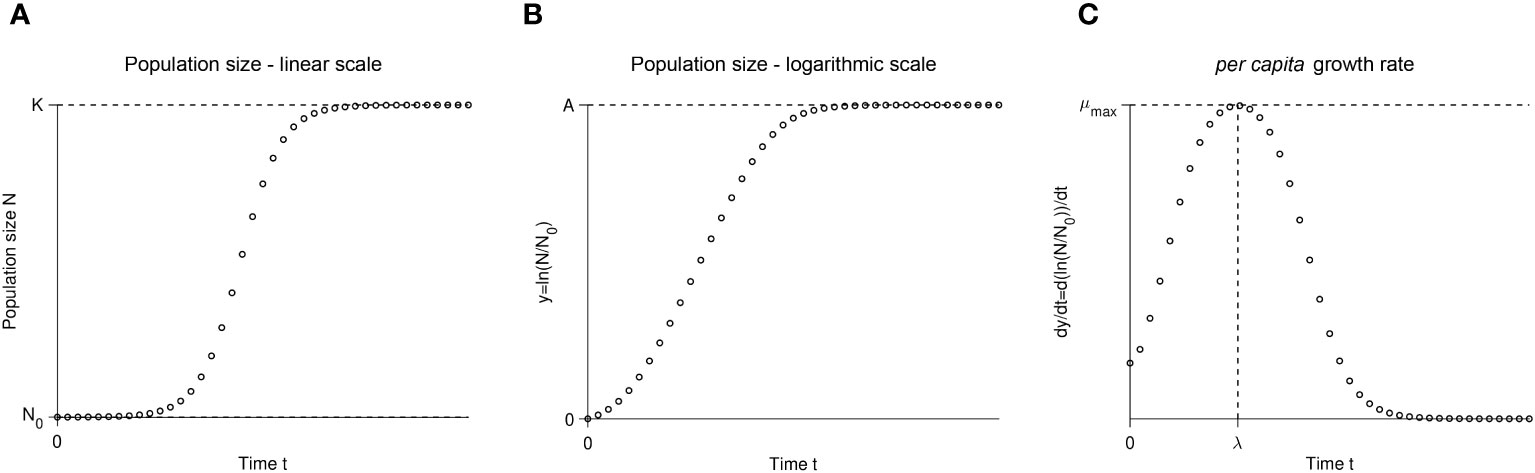
Figure 1 A schematic illustration of the same simulated batch culture population growth curve, plotted in three different ways. (A) Population size N versus time t. The quantity K corresponds to the carrying capacity and N₀ to the initial population size. The initial population fraction is given by N₀/K. (B) Logarithm of the population size divided by the initial population size y = ln(N/N₀) versus time t. Note that in other publications, the quantity ln(N/N₀) is sometimes denoted as y. The quantity A = ln(K/N₀) is the logarithm of the fold increase over the initial population size at carrying capacity. (C) First derivative of the logarithm of the population size divided by the initial population size dy/dt = d ln(N/N₀)/dt versus time t. The function dy/dt may be interpreted as the per capita growth rate. The quantity µ_max is the per capita maximum growth rate and λ the lag phase duration.

Growth curves are often used to estimate the per capita growth rate and fitness. The per capita growth rate is important in population biology because it is used to calculate the growth of a mutant strain compared to a wild-type strain: the relative growth rate or the relative fitness (w). The relative fitness is particularly important in evolutionary biology since it classifies a mutant as deleterious (w< 1), neutral (w = 1), or beneficial (w > 1) with respect to natural selection. Indeed, when the relative fitness is greater than 1, the mutant reproduces faster than the wild-type, and conversely, when w is less than 1. Although there is still discussion in the field about whether the relative growth rates measured from monoculture growth curves are predictive of competitive fitness (Concepción-Acevedo et al., 2015; Ram et al., 2019), many biologists use the growth rate as a measure of fitness (e.g., Knopp and Andersson, 2018).

Microbial batch culture protocols have been used for over 100 years in microbiology (e.g., Slator, 1916) and population ecology (e.g., Carlson, 1913) and remain a mainstay of experimental evolution and ecology. During this time, many experimental protocols (Delaney et al., 2013; Hall et al., 2014; Stevenson et al., 2016; Kurokawa and Ying, 2017) and estimation methods (Zwietering et al., 1990; Baranyi and Roberts, 1994; Jung et al., 2015) have been developed for this type of data. Since the early 1990s, automated plate readers that incubate and periodically scan the opacity of the cultures growing in the microwells have simplified the process of gathering data for hundreds of bacterial populations simultaneously growing in (relatively) homogeneous batch culture environments. Sources of inconsistency, like the batch effect (Blomberg, 2011), can be mitigated, for example, by growing all cultures of interest on the same day(s) to arrive at consistent data. Nevertheless, despite the long tradition and good recommendations for setting up experiments, programs and papers detailing methods for estimating growth rates (and other growth parameters) from this data continue to be published and highly sought after. Many of these estimation methods implement classical models (e.g., Sprouffske and Wagner, 2016; Petzoldt, 2020). This shows that after 100+ years of generating growth curve data, microbial ecologists and evolutionary biologists are still struggling to find the best way of estimating the growth rate from their data.

The main goal of our paper is to demonstrate that there are significant limitations to existing methods for using batch culture growth curve data to estimate the intrinsic growth rate µ, which is the fastest per capita number of divisions per time unit theoretically possible when the cell’s resources are infinite or otherwise optimal. These limitations impact the calculation of quantities of interest, such as the selection coefficient and the relative fitness. We first take stock of how the community analyzes growth curve data by semi-quantitatively reviewing the literature to survey which methods are used in evolution and ecology. After explaining different approaches for modeling growth curves, we use math and simulations to show that many currently used approaches are inappropriate for accurately estimating the intrinsic growth rate µ. We quantify the errors for the intrinsic growth rate µ when the maximum observed growth rate µ_max is used as an estimator and the generating model is known. Next, we present the limited set of conditions in which an exponential approximation can be used for estimating µ. Importantly, we demonstrate that using inaccurate estimates of µ to estimate the relative fitness often leads to inaccurate fitness estimates and sometimes even wrongly classifying a beneficial mutation as deleterious. Finally, we apply our theoretical insights to previously published data and show that absolute and relative growth rate estimates may vary greatly depending on the method. Overall, we present a systematic evaluation of different methods, with recommendations for best practices.

2 Results & discussion

2.1 Literature review: How does the community analyze the data?

We reviewed 50 papers from evolution and ecology that estimated growth curves for all types of microbial data (see Table S1 and Methods section).

Most of the data (90%) were acquired by an automated microplate reader tracking optical density (OD) over time. Other data types included cell counts or fluorescent yields over time. Several papers (6%) did not report the starting inoculum size. Of those papers that reported the inoculum size, 52% used a fixed absolute initial population size ( $\widehat{N_0}$) for inoculation, whereas 44% had a variable absolute initial population size because the inoculating-culture was diluted by some fixed dilution factor (i.e., $\widehat{N_0}=\widehat{K}\times dilutionfactor$). For the latter type of experiments, the absolute population size of the inoculum, N₀, differed between strains/treatments when the carrying capacities, K, were different. The reported dilution factor varied between 10⁻⁴ to 10⁻¹ with a geometric mean value of 10^−2.37.

We found that the growth rate was by far the most commonly estimated growth parameter (94% of all papers reviewed). The other estimated growth parameters were the carrying capacity (44%), the lag time (34%), and the area under the curve (AUC; 12%). The growth rate was usually reported as an absolute value for each strain/treatment. Moreover, 24% of papers estimated the relative growth rate, or relative fitness, of different strains as compared to the wild-type.

Methods that explicitly fit a model of population growth were used about as often as “model-free” or “nonparametric” approaches (i.e., methods that do not require a model; Figure 2A). One particular model-free approach, the “Easy Linear” method, was especially popular (right doughnut chart of Figure 2A): it was used in about a third of all papers. When models were used, only one model was usually reported to have been fit (left doughnut chart of Figure 2A).

Figure 2

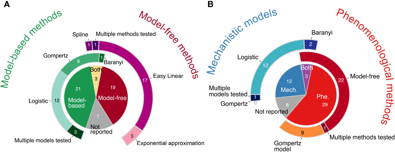
Figure 2 Pie and doughnut charts of literature review results. (A) Model-free methods were used about as often as model-based methods across all 50 papers reviewed. “Both” refers to when both a model-free and a model-based method were used in the same paper. The doughnut charts surrounding the central pie chart illustrate how frequently different models, including both phenomenological and mechanistic models, were used (left, shades of green) and how frequently different phenomenological model-free methods were used (right, shades of purple). (B) Phenomenological approaches (Phe) were used more often than mechanistic models (Mech). “Both” refers to when both a mechanistic model(s) and a phenomenological approach(es) were used in the same paper. The doughnut charts surrounding the central pie chart illustrate how frequently different mechanistic models were used (left, shades of blue) and how frequently different phenomenological approaches were used (right, shades of red-orange). The Gompertz model is listed twice because it is either a mechanistic model or a phenomenological model, depending on the equation; however, no paper was found to use a mechanistic Gompertz model. Both of the phenomenological Gompertz models listed in Table 1, Gompertz and modified Gompertz, are grouped together. For more details on the methods and equations used by each paper, see Table S1. Slices within each pie and doughnut chart show the counts of papers included.

We classified the growth curve analysis methods as either mechanistic or phenomenological (Figure 2B). A mechanistic model estimates the intrinsic growth rate, µ, and allows researchers to simulate the underlying process. In contrast, a phenomenological approach enables researchers to estimate the maximum growth rate, µ_max, and describe/quantify the pattern of interest but without simulating the underlying process (see next section). We found that phenomenological approaches were used more often than mechanistic models (Figure 2B). The most popular methods within the phenomenological approach were the various model-free methods (right doughnut of Figure 2B). The logistic model was by far the most popular mechanistic model used (left doughnut of Figure 2B). Depending on its equation, the Gompertz model is either a phenomenological or a mechanistic model (Table 1); however, we found that the mechanistic Gompertz model was never fitted, whereas the phenomenological Gompertz model was popular (18% of all papers and 28% of all phenomenological methods used).

Table 1

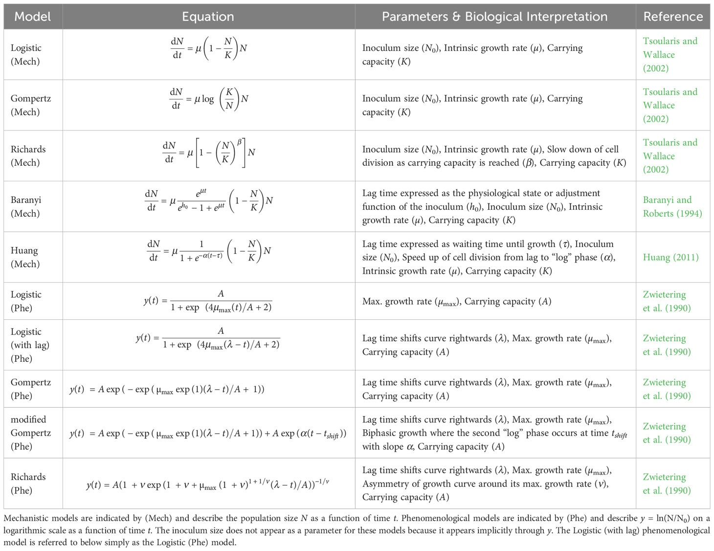
Table 1 Different population growth models: The population growth models considered in this paper with their equation and parameters.

We found that many growth curve experimental methods, data, and analyses do not yet conform with recommendations for reproducible research (e.g., Wilkinson et al., 2016; Munafò et al., 2017). Over 10% of the papers reviewed reported insufficient information about how growth curves were analyzed and therefore could not be classified for Figure 2. Some highly-cited papers (e.g., Gullberg et al., 2011; Trindade et al., 2012) neither cited an established method nor included a sufficient description of their ad hoc methods for estimating growth rates (see Table S1). Beyond reporting of experimental methods, the data set itself was often not shared: about half (46%) of all papers do not show any figures of nor provide any of the growth curve data (see Table S1). 40% of papers provided plots of at least a subset of the growth curves, and 14% of all papers published their raw growth curve data.

Our finding from Figure 2 that ∼13% of articles provide insufficient information regarding their growth curve analysis methods likely underestimates the magnitude of the problem. This is because we found articles for inclusion in the review by searching among the citations to previously published growth curve analysis methods papers (see Methods). Therefore, most of the papers we included cited an established method for analyzing growth curve data. Hopefully, these issues of methods under-reporting will improve as scientists become more knowledgeable about recommendations for open science and data management (Wilkinson et al., 2016; Munafò et al., 2017).

Our finding of insufficiently reported information regarding the analysis of growth curves corroborates previous concerns about the lack of a standard method for growth curve analysis (Fernandez-Ricaud et al., 2016). The remainder of our article discusses different methods for analyzing growth curves and, thus, will hopefully contribute to an increased appreciation of why it is important to provide sufficiently detailed methodological information on data analyses.

2.2 Exposition of existing models and methods

2.2.1 Conceptual distinctions between parametric vs non-parametric methods and phenomenological vs mechanistic models

A variety of approaches have been developed over the years to describe and quantify growth curves, as shown in Figure 2. Below, we explain the main differences between the most commonly used approaches and models. Then, we compare the advantages of each.

2.2.1.1 Model-free vs model-based methods

One way to classify the different methods is to distinguish between model-free (or non-parametric) methods and model-based (or parametric) methods. Model-free methods use an algorithm to find an estimate of the growth rate that is relatively robust to any noise error in the data. For example, in the classical exponential approximation from Monod (1949) that is featured in many introductory microbiology textbooks, the growth rate is estimated by measuring cell concentrations (N₁ and N₂) at two time points (t₁ and t₂) during the “log phase” of growth, then calculating R = (log₂ N₂ − log₂ N₁)/(t₂ − t₁). This is an algorithm that can easily be used by hand or performed by a computer. The Easy Linear method (Hall et al., 2014; Mira et al., 2017) is a more complex algorithm that uses a sliding window of five successive data points to calculate the maximum slope among many linear regressions fitted to the log-scale growth curve data. Another example is the Spline method that calculates the maximum value of the first derivative of the log-scale growth curve data by either using the mean of three successive pairs of points (e.g., Ashino et al., 2019) or kernel smoothing of the growth curve (e.g., Kahm et al., 2010; Petzoldt, 2020) to remove experimental noise. The parameters of these algorithms are usually tunable, for example, the size of the sliding window used by the Easy Linear method. Although no explicit assumptions are made about the shape of the growth curves, all of the examples cited above rely on the implicit assumption that the data is in the exponential growth phase. Also methods that ostensibly make no assumptions (e.g., Midani et al., 2021) extract particular summary statistics of interest from the data (e.g., the maximum observed per capita growth rate).

On the other hand, model-based methods use equations to describe the relationship between time explicitly, the independent variable, and population size (or a proxy of population size, like OD), the dependent variable. A model-fitting algorithm is then used to find the model parameters that best fit the observed data, usually by minimizing the residual sum of squares. Model-based methods tend to be preferred by theoretical and statistical biologists because models specifically define the assumptions that are being made, model-based methods have defined protocols for assessing goodness of fit, and model-fitting allows quantification of the (frequentist or Bayesian) error of the estimates (Bolker, 2008; Otto and Day, 2011). Nevertheless, methods with explicit models can still hide their assumptions and, worse still, may introduce a level of abstraction that prohibits productive discussions between theoreticians and empiricists.

Empiricists tend to prefer to apply model-free approaches to biological growth curve data both because it is technically more difficult to fit and compare models and because of the inflexibility of existing models to fit the data (source: personal communication). In other words, the main advantage of model-free approaches is that they do not require a model. Model-free approaches have drawbacks, however: since there is no model, it is not clear how to compare the likelihood or goodness-of-fit between different methods, and bootstrapping is necessary to quantify the error around estimates (for example, to generate confidence intervals).

2.2.1.2 Mechanistic vs phenomenological models

Within the class model-based methods, there is a difference between mechanistic and phenomenological models. Mechanistic models may also be called process models, and phenomenological models can be called statistical/pattern models (Bolker, 2008; Liberles et al., 2013). We define mechanistic models as representations that simulate or at least bear some resemblance to the underlying process(es) that produced the data. Therefore, the parameters estimated from mechanistic models are interpretable with respect to the underlying process. For population growth curve models in particular, the per capita growth rate of a mechanistic model is, by definition, the intrinsic growth rate µ when the cell’s resources are limitless or otherwise optimal.

Phenomenological models can be thought of as ‘black-box empirical models’ (Chezeau and Vial, 2019). They are created by selecting functions that have a similar shape as the pattern of interest. Then, the parameters of those functions are given a biologically relevant meaning. For growth curves in particular, phenomenological population growth models are defined such that the point on the curve with the fastest rate of per capita growth (i.e., the inflection point of y = ln(N/N₀)) corresponds to the maximum growth rate µ_max (Zwietering et al., 1990, equations 4 & 5). Model-free (non-parameteric) methods all belong to the phenomenological category, as shown in Figure 2B, as they quantify specific parameters of interest without simulating the underlying process.

Although the distinction between mechanistic models and phenomenological methods may seem arcane, it is crucial because parameters estimated from phenomenological methods cannot be treated as unbiased estimators of parameters for mechanistic models (Rodrigue and Philippe, 2010). We explain below how serious pitfalls in estimating growth rates are a direct result of the differences between growth rates estimated by mechanistic models (i.e., the intrinsic growth rate µ) and phenomenological methods (i.e., the maximum growth rate µ_max).

2.2.2 Biological interpretation of commonly used models and their parameters

We summarized the equations and parameters of the most prevalent models found by our literature review in Table 1, distinguishing mechanistic models (Mech) from phenomenological models (Phe). As mentioned above and further explained in the next section, a main difference to note is that mechanistic models are defined in terms of the intrinsic growth rate µ. In contrast, phenomenological models are defined in terms of the maximum growth rate µ_max.

The common feature of all models listed in Table 1, whether mechanistic or phenomenological, is that they assume an exponential phase of growth eventually followed by a cessation of growth as the carrying capacity is reached. In other words, the models assume that the data has a sigmoid or “S” shape (Zwietering et al., 1990). All models consider single-strain, well-mixed bacterial populations starting with an inoculum (i.e., initial population) size of N₀ microbes. Every individual in the population is assumed to divide at the same per capita rate, although the division rate varies over time.

The models differ in important ways. Most of the models are based on the logistic model but seek to add additional features (Tsoularis and Wallace, 2002). For example, a lag phase can be added to the phenomenological Logistic model by adding a parameter (λ) that shifts the curve towards the right (Table 1). In contrast, the Baranyi model adds a mechanistic lag phase to the model by including a parameter (h₀) that describes the physiological state of the inoculum (Baranyi and Roberts, 1994, Baranyi and Roberts, 1995). When cells go from a saturated culture to a fresh culture or otherwise change their environment, this adjustment function describes the build-up of a critical cellular substance to a threshold necessary for cell growth. The Huang model, another mechanistic model with a lag phase, describes a similar lag phase as the Baranyi model but uses a less detailed process.

Similarly, there are different ways to model population growth at high densities. For example, the Richards model (mechanistic or phenomenological) includes a parameter (β or ν, respectively) that changes how the per capita growth rate slows down from its maximum value to the stationary phase. Therefore, the mechanistic β parameter in the Richards model incorporates processes that occur at high cell density (i.e., due to changes in the media environment or other intra-specific density-dependent effects). Finally, Gompertz models differ from Logistic models by assuming a different process for how the population approaches its carrying capacity. Namely, Gompertz models have a higher per capita growth rate but approach the carrying capacity more slowly than Logistic models for the same set of parameters. We stress that during experiments, violation of the Beer-Lambert law and changes in cell size at high density can lead to spurious inference of complex phenomena like those listed above when optical density data has not been calibrated appropriately to cell counts (Stevenson et al., 2016).

2.2.3 What is the difference between µ and µ_max?

It is important to distinguish between three growth rate estimators: the maximum population growth rate (max (dN/dt)), the per capita maximum growth rate (µ_max), and the per capita intrinsic growth rate (µ). The maximum population growth rate (max (dN/dt)) is the fastest increase in size achieved by the entire population. We are not interested in the maximum population growth rate parameter since it is not estimated by any of the methods or models we discuss here; we only mention it so that the reader does not mistake it for the maximum growth rate (µ_max). The maximum growth rate µ_max is the fastest per capita number of divisions per unit of time actually achieved in the observed growth curve. In more quantitative terms, µ_max is the maximum value of the curve d ln(N/N₀)/dt (Figures 1B, C). As mentioned above, the maximum growth rate µ_max is a value estimated using phenomenological approaches. Finally, the intrinsic growth rate µ (sometimes denoted as r (Sprouffske and Wagner, 2016), called the Malthusian parameter of population growth, or the intrinsic rate of increase) is the fastest per capita number of divisions per unit of time theoretically possible and, because it is a mechanistic model parameter, it is used for simulating population growth processes. We here focus on the intrinsic growth rate µ and the maximum growth rate µ_max because these are the two quantities estimated by the most used methods.

An important conceptual difference exists between the intrinsic growth rate µ and the maximum growth rate µ_max. The intrinsic growth rate µ is the theoretical maximum number of cell divisions per time unit, assuming population dynamics that follow an exponential law. Importantly, µ is an idealized parameter. No real population achieves an infinite size because the division process is limited by space and/or nutrients, for instance. Thus, the number of divisions per time unit is not constant over time, so the maximum division rate µ_max is the largest per capita value observed during the population growth. Therefore, the intrinsic growth rate µ can quantify the strain-specific division rate theoretically independently of the environment or experimental conditions. On the other hand, the maximum growth rate µ_max (like other values estimated by phenomenological methods) is always specific to the experiment itself and cannot be generalized as a strain-specific value that applies to different environments or conditions. As will be shown below, in the best case scenario, µ_max approximates µ, but in other scenarios, µ_max is a composite parameter that depends on other values like the inoculum size and lag time.

Previous work has pointed out confusions between different growth rate estimators (Perni et al., 2005). The confusion between these terms is so prevalent that some papers mistook µ for µ_max (Yang et al., 2006), vice versa (Wu et al., 2017), or distinguished between the two but swapped the names (Khan et al., 2017). Furthermore, some authors wrote the mechanistic logistic equation as dN/dt = µ_max(1 − N/K)N (Petzoldt, 2020), whereas other authors preferred dN/dt = µ(1 − N/K)N and µ_max = max(d ln(N(t)/N₀)/dt) (Sprouffske and Wagner, 2016). Different naming conventions become even more misleading for models in which the intrinsic growth rate is a function of the resource concentration, such as the Monod class of models that have their own specific, mechanistic definition for µ_max (Monod, 1949; Chezeau and Vial, 2019). We will not discuss substrate-use models herein. Having explained the conceptual differences between the µ_max maximum growth and µ intrinsic growth rates above, we now expand on the mathematical differences.

2.2.3.1 Deriving the difference between µ_max vs µ

In the following, we mathematically explain why µ_max is not always a good proxy for µ, especially at large initial population fractions, N₀/K. Analytical math is combined with simulations to show for which initial population fractions an experimenter can estimate the intrinsic growth rate µ from the maximum growth rate µ_max.

We assumed that the population dynamics follow one of the mechanistic growth models from Table 1 and mathematically derived µ_max for the five mechanistic models. As reported in Table 2, µ_max depends on the system parameters, namely the initial population fraction N₀/K as well as the parameters β and h₀ for the Richards and the Baranyi models, respectively.

Table 2

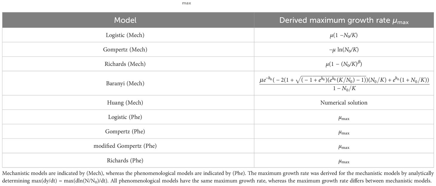
Table 2 Maximum growth rates: The maximum growth rate µ_max for the population growth models considered in this paper.

The results of Table 2 are illustrated by the points in Figure 3A. The estimated maximum growth rate (µ_max) values differ between models with the same parameter values (intrinsic growth rate µ = 1 and carrying capacity K = 10⁵). In general, the maximum growth rate is approximately equal to the intrinsic growth rate when the initial population fraction satisfies $N_0/K\ll 1$ and ${(N_0/K)}^{\beta }\ll 1$ in the Logistic and Richards models, respectively. Indeed, these conditions lead to µ_max = µ(1 − N₀/K) ≈ µ and µ_max = µ(1 − (N₀/K)^β) ≈ µ for the Logistic and Richards models, respectively (see Table 2). The Gompertz model is a special case since the maximum division rate is a good proxy for the intrinsic division rate when the initial population fraction is large, roughly equal to exp(−1) ≈ 0.37 (i.e., an inoculum size corresponding to a dilution factor for the stationary phase batch culture of between one-third and two-fifths).

Figure 3

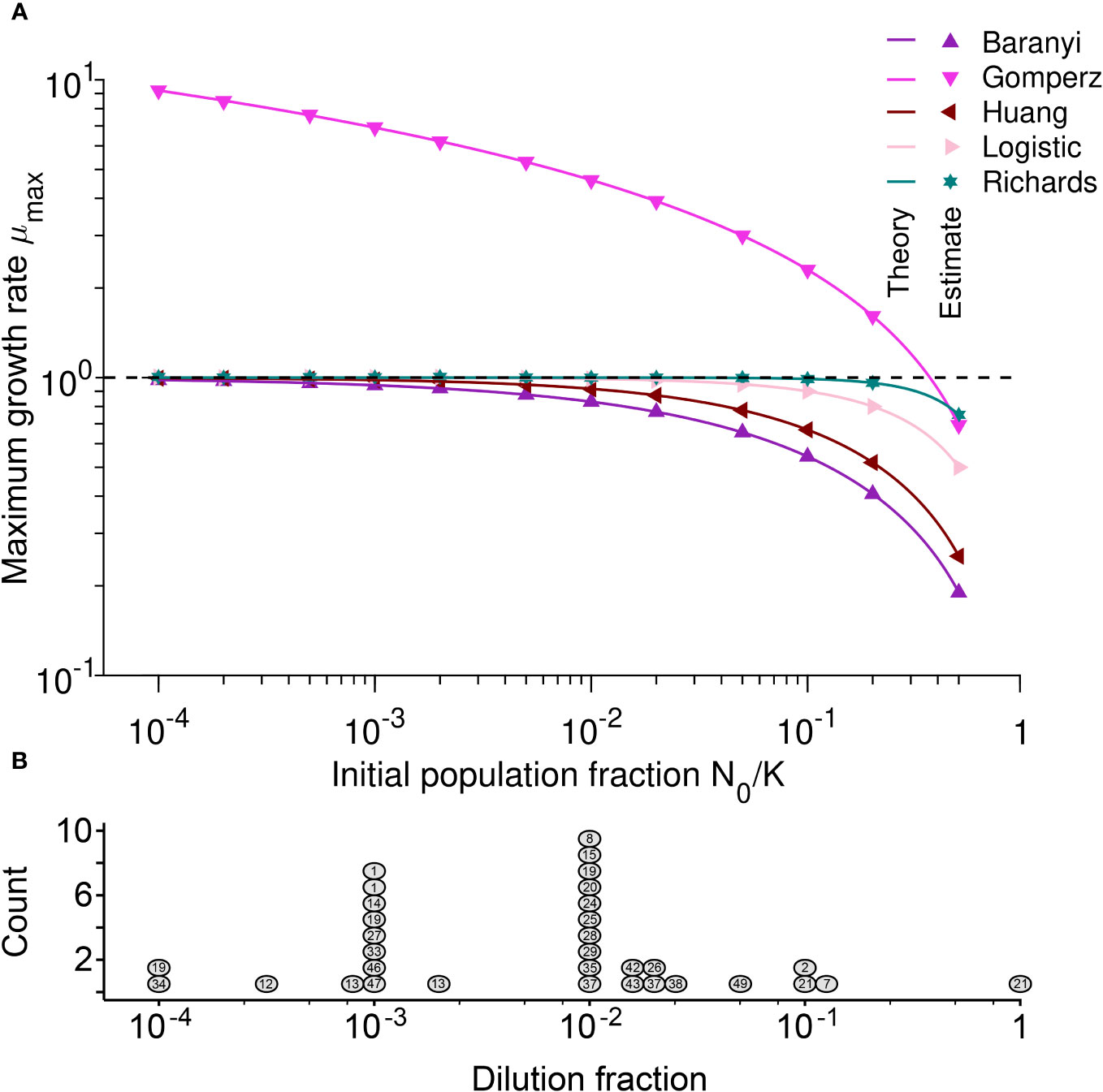
Figure 3 (A) The Gompertz model and large initial population fractions make the maximum growth rate a poor proxy for the intrinsic growth rate: Maximum growth rate µ_max versus initial population fraction N₀/K for different mechanistic population growth models, where µ = 1. Each point represents estimated values by Spline (from Petzoldt, 2020) from simulated data averaged over 10⁴ stochastic realizations. The solid lines correspond to the analytical predictions of the maximum growth rate (see Table 2). The dashed line shows the intrinsic growth rate value µ. Parameter values: K = 10⁵, µ = 1, α = 2, β = 2, h_{0 =} 2 and τ = 2. (B) For the most commonly used dilution fractions in the literature, the maximum growth rate is a good proxy for the intrinsic growth rate: Histogram of the estimated dilution fractions observed for the 27 (out of 50) papers that provided sufficient information to estimate this value. Each circle represents a publication, and the number inside the circle indicates the number of the reference, as given in Supplementary Table S1. Several publications appear more than once because they used more than one dilution fraction for different experiments.

In order to test the analytical predictions from Table 2, we evaluated the growth rates as estimated by model-free methods using data simulated under each of the five population growth models. Unlike experimental data, for which the true µ value that generated the data is never known, estimating the growth rate from simulated data allowed us to check the accuracy of the estimates as compared to the known µ parameter that the data was simulated under.

We focus on two model-free methods, the popular Easy Linear (Hall et al., 2014) and the Spline (e.g., Adkar et al., 2017; Ashino et al., 2019) methods, to determine the maximum growth rate µ_max. Both methods assume that only the exponential stage of growth is useful to estimate the maximum growth rate. We generated data using individual-based stochastic simulations for the Gompertz, Richards, Logistic, Huang, and Baranyi models. Then, we used the two different model-free methods, Spline and Easy Linear, to compute the maximum growth rate µ_max for different parameter values. In practice, both model-free methods provided us with the same results. That is because our simulated data, averaged over several stochastic realizations, did not include the myriad sources of noise present in experiments.

As shown by the lines in Figure 3A, there is an excellent agreement between our analytical predictions (lines) and the estimates from simulated data (points). As predicted analytically, the estimated maximum growth rate µ_max does not equal the known intrinsic growth rate µ value used to create the simulations unless $N_0/K\ll 1$. For the Baranyi, Huang, Logistic, and Richards models, the smaller the initial population fraction, the better the maximum growth rate performs as a proxy for estimating the intrinsic bacterial growth rate, µ. However, this is not the case for the Gompertz model. For the Baranyi and Richards models (Supplementary Figures S4A, B), the smaller the parameter h₀ and the larger the parameter β, the closer is the maximum growth rate µ_max to the intrinsic growth rate µ. Similarly, for the Huang model, the higher the curvature defined by α and the shorter the duration τ of the lag phase, the better µ_max is as a proxy for µ (see Figures S4C, D).

We showed that the maximum growth rate µ_max is not always equivalent to the intrinsic growth rate µ. Therefore, methods that estimate the maximum growth rate µ_max but then (often implicitly) assume that this value can be treated as the µ of a mechanistic model must be applied with caution. As we have demonstrated in Table 2 and Figure 3A, µ_max tends to underestimate the true intrinsic growth rate µ – except when population growth follows the Gompertz mechanistic model, in which case the maximum growth rate µ_max mostly overestimates the true intrinsic growth rate µ. This is because the per capita growth rate is generally smaller than the intrinsic one. Hence, we recommend that a clear distinction must be made between the intrinsic growth rate µ and the maximum growth rate µ_max.

2.2.3.2 The initial population fraction, N₀/K, is a key parameter determining the relationship of µ_max and µ

Above, we showed that (for most models) we can use the estimated maximum growth rate µ_max as an approximation of µ when initial population fractions N₀/K are small. We estimated the dilution fractions used in different experiments (Figure 3B) to ascertain whether most studies are using appropriately small initial population fractions. Papers reporting experiments with multiple, different batch culture starting conditions are included as multiple points with the same number. For example, Ganucci et al., 2018 (labeled as 21) used a dilution fraction near 1. The authors used cell viability counts to track yeast growth in media with increasing ethanol concentrations, sometimes resulting in almost no growth. Two values from Ganucci et al. (2018) are summarized in Figure 3B, indicating the largest (0.1) and the smallest (0.94) dilution fractions observed. Since methods differ between publications, with some using a mid-exponential phase culture and others using a stationary phase culture for inoculation (see Supplementary Table S1), the estimated dilution fraction should be considered as an upper bound for the initial population fraction used in each paper.

More than two-thirds of papers use at least one estimated dilution fraction smaller than 10⁻²; the geometric-mean observed dilution fraction was 10^−2.7. For such small dilution fractions, if there is no lag time, and if growth follows one of the population growth models except Gompertz, the maximum growth rate µ_max tends to be a good estimator of the intrinsic growth rate µ. When the true growth curve dynamics in the experiments follows one of the mechanistic models other than Gompertz, the relative difference between the maximum growth rate and the intrinsic growth rate for the mean initial population fraction N₀/K = 10^−2.7 is between 0-12%. Here, the largest difference between µ_max and µ is obtained for the Baranyi model. However, for the Gompertz model, the relative difference between the maximum growth rate and the intrinsic growth ranges from -821% to 31% (see Figure 3).

2.2.3.3 Consequences of the difference between µ_max and µ

We showed that the µ_max values calculated from mechanistic models depend on other parameters in addition to µ, such as the initial population fraction. Conversely, one cannot obtain µ from µ_max alone. For mechanistic models, additional parameters such as the initial population size and carrying capacity are required (see Table 1) to be able to calculate µ from µ_max. For phenomenological approaches, which are specified directly in terms of µ_max, µ is not defined. Nevertheless, even when µ_max is estimated by phenomenological models, its estimated value will be different when experimental quantities such as the initial population size and carrying capacity change. In reality, the estimated values for both µ_max and µ may also vary with the experimental conditions (such as genotype, medium, temperature, etc).

We emphasize that the main difference between the maximum growth rate µ_max and the intrinsic growth rate µ is that µ_max is a phenomenological quantity, whereas µ is a model parameter. Therefore, obtaining different estimates of µ and µ_max is expected and not a sign of bad performance of a model or method, especially for large initial population fractions. For example, the manual of one software (Delaney, 2014) provides options for fitting various phenomenological models and a single mechanistic model but discourages users from applying the mechanistic model because “it predicts fastest growth” as compared to the other implemented models. Our results can readily explain this observation and debunk the implied worse performance of the mechanistic model. Indeed, the publication associated with this software recommends a large inoculum size (Delaney et al., 2013; associated studies labeled as 8, 22, 25, 42, and 43 in Figure 3B and Supplementary Table S1), for which we showed that µ_max should consistently overestimate µ.

Given the differences between µ_max and µ, which should be estimated? Unfortunately, there is no one-size-fits-all answer to this question. From a theoretician’s perspective, one might recommend that researchers estimate the intrinsic growth rate µ. Most studies perform growth curve experiments to characterize growth for specific strains, treatments, or environments in the (either explicit or implicit) context of population ecology or mechanistic models, defined in terms of µ. Only the intrinsic growth rate µ can be used to simulate mechanistic models and identify the mechanisms that best explain the observed dynamics. On the other hand, the maximum growth rate µ_max is phenomenological: it describes what is observed in the data contingent on the population’s starting conditions and the experimental environment. At best, µ_max approximates µ. However, from an experimenter’s perspective, estimating µ_max has the advantage that model-free methods are technically easier to use than estimators of mechanistic models, especially for data that displays an uncommon trend (e.g., biphasic growth) different from the usually modeled exponential or “S”/sigmoid shapes. We strongly encourage researchers who decide to estimate µ_max to use (and report) a small initial population fraction and to assert that the data does not have a significant lag time.

When using phenomenological methods, a second decision about whether to use model-based or model-free methods is necessary. In our noise-free, simulated data, model-based and model-free phenomenological methods yielded the same estimates for µ_max (Figure 3A); future work should elaborate on their performance in the presence of different sources of noise (e.g., to expand previous work by Mira et al. (2017) for the Easy Linear method). Although model-based methods may be preferable from a theoretician’s view, certain types of experimental data (for example, displaying biphasic growth, curves without samples in the stationary phase, and other unusually shaped data as well as very noisy data) may not be fitted well by models of exponential or sigmoidal growth. In this case, the data may be better summarized by a model-free phenomenological method. Importantly, we recommend that the choice of method is justified clearly and in writing, no matter which method is used.

2.3 Guidelines for estimating growth rates

2.3.1 Ad-hoc fitting of an exponential model to growth curves should be avoided

One common approximation (Monod, 1949; Kassen, 2014) that is used to obtain an estimate of the intrinsic growth rate µ is to fit an exponential equation, like N(t) = N₀e^µt, to the early phases of growth (i.e., during the “log” phase, before the deceleration and stationary phases). This method is explained in many introductory microbiology textbooks, as previously summarized in the explanation of model-free methods in section 2.2.1 above, and we refer to this approach as an exponential approximation. Under the exponential approximation, the intrinsic growth rate is given by µ = ln(N(t)/N₀)/t.

To test the accuracy of the exponential approximation when applied to batch culture population growth, we expressed the intrinsic growth rate as a function of population size and other possible parameters for different mechanistic population growth models (Table 3 and Supplementary Figure S5).

Table 3

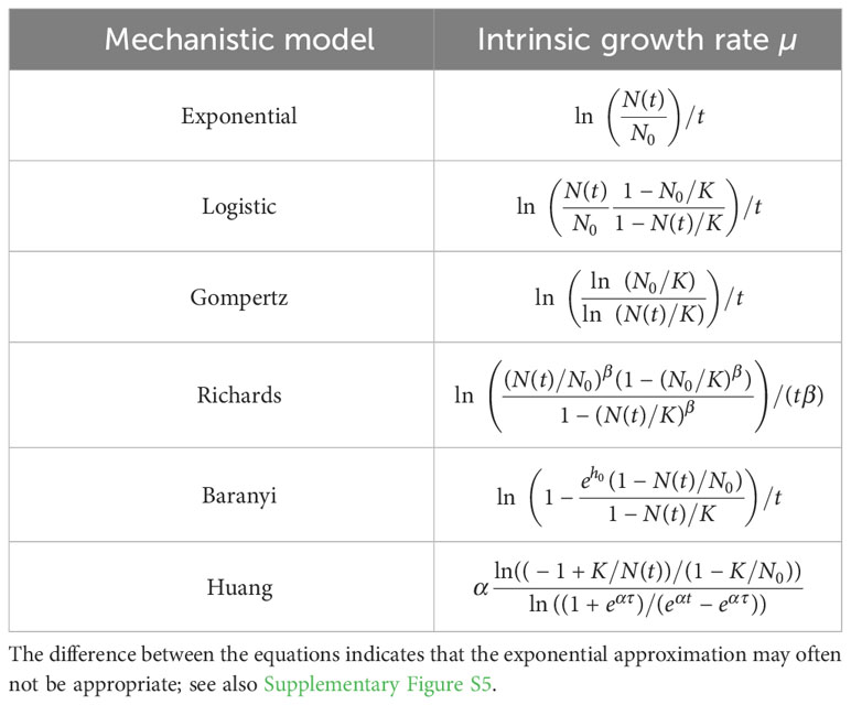
Table 3 Intrinsic growth rate as a function of the model parameters at time t for different mechanistic population growth models.

We found that the exponential approximation is frequently a poor estimator of the intrinsic growth rate µ. The exponential approach is never valid for a population following the Gompertz growth. There is no parameter range for which the equation ln(ln(N₀/K)/ln(N(t)/K))/t reduces to ln(N(t)/N₀)/t (see Table 3). The exponential approach is valid for the logistic growth when the initial population size is very small in comparison to the carrying capacity (i.e., $N_0\ll K$) and for time points at which the population size remains small in comparison to the carrying capacity (i.e., $N(t)\ll K$). These conditions lead to ln(N(t)(1 − N₀/K)/(N₀(1 − N(t)/K)))/t ≈ ln(N(t)/N₀)/t (see Table 3). This makes sense since the phase during which these conditions are satisfied corresponds to the regime in which logistic growth can be reduced to exponential growth. The same conditions apply to Baranyi growth, with the additional condition that the lag phase must be short (i.e., $h_0\ll 1$), so that one obtains ln $1-e^{h_0}(1-N(t)/N_0)/(1-N(t)/K))/t\approx \ln (N(t)/N_0)/t$ (see Table 3). If the lag phase is not short, the exponential phase starts later, whereas the exponential approach assumes that it starts at the beginning of the growth. The Richards growth is more complex. Here, the quantities (N₀/K)^β and (N(t)/K)^β must be much less than 1 to make the exponential approach valid. The larger the deceleration parameter β is when $N_0\ll K$ and $N\ll K$, the more abruptly the “log” phase transitions into the stationary phase, and the more valid the exponential approximation becomes, so that $\text{ln}{((N(t)/N_0)}^{\beta }(1-{(N_0/K)}^{\beta })/(1-{(N(t)/K)}^{\beta }))/(t\beta )\approx \text{ ln}(N(t)/N_0)/t$ (see Table 3). Consequently, the exponential approximation is valid only in a very restricted set of conditions: when there is no lag phase, the initial population fraction is very small, and the measured population sizes remain small as compared to the carrying capacity. Most experimental data probably does not meet this necessary set of conditions.

It is of note that throughout the literature, including introductory textbooks, the term “exponential growth rate” tends to be used to describe the intrinsic growth rate µ and is sometimes deemed the same as the maximum growth rate µ_max (e.g., Novak et al., 2009; Basra et al., 2018). We here strongly caution against this conflation of potentially very different quantities. In particular, we recommend that approximating batch culture growth with an exponential curve to get an estimate for the intrinsic growth rate µ requires careful assurance that the assumption is valid for the data at hand.

2.3.2 Theory predicts that using µ_max or the exponential approximation for estimating relative fitness can yield wrong results

In evolution and population biology, the relative fitness w of a mutant strain (M) compared to a wild-type strain (WT) is classically defined as the ratio of their intrinsic growth rates, µ^M/µ^WT. The relative fitness or the selection coefficient, defined as s ≡ w−1 = µ^M/µ^WT −1, is used to classify a mutant as deleterious (w < 1 or s < 0), neutral (w = 1 or s = 0), or beneficial (w > 1 or s > 0). Thus, to infer how natural selection favors one strain over another from monoculture growth curves, microbial ecologists and evolutionary biologists need to estimate the intrinsic growth rate, which is obtained by fitting a mechanistic model.

It is often argued that the concerns regarding miscalculation of the intrinsic growth rate µ discussed above are important for absolute growth rate estimates but can be disregarded when considering relative estimates. The argumentation is that whereas absolute estimates cannot be compared between data sets, relative growth rates can be estimated within a data set by using a common reference sample, and these relative growth rates can then be compared between data sets. Moreover, the sign of an estimated selection coefficient may be more important than the absolute value. Namely, incorrect absolute estimates should yield correct rankings of growth rate estimates and thus correctly estimated signs of the selection coefficient. Below, we demonstrate that these assumptions are wrong and that incorrect estimates of the growth rates (for example, by assuming that µ_max = µ) can severely affect the classification of strains into beneficial, neutral, or deleterious.

To demonstrate the effects of assuming µ_max = µ on relative fitness estimates, we simulated growth curve data from separate batch monocultures for two strains. We estimated their maximum growth rates µ_max using the growth curves. Then, we assumed (erroneously) that the maximum growth rate µ_max was a good approximation of the intrinsic growth rate µ. We calculated the relative fitness of the mutant with respect to the wild-type as $w={\mu }_{\max }^M/{\mu }_{\max }^{WT}$ (or the selection coefficient as $s={\mu }_{\max }^M/{\mu }_{\max }^{WT}-1$).

Figure 4A shows that using µ_max to estimate the relative fitness generally infers incorrect values for the relative fitness (as well as the selection coefficient), unless both strains have the same initial population fraction (N₀/K). Even more concerningly, this estimation sometimes categorizes the mutant as deleterious when it is beneficial and vice versa. This is especially problematic because we assumed noise-free data and an ideal case in which both bacterial strains followed the same population dynamics. In summary, we conclude that equivocating µ_max with µ will likely lead to wrong fitness and selection coefficient estimates.

Figure 4

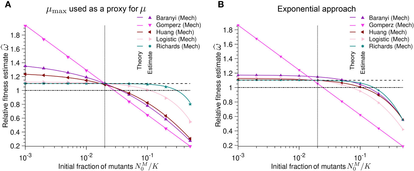
Figure 4 Different initial population fractions between wild-type and mutant batch cultures result in poor estimates of relative fitness: Relative fitness $\widehat{\omega }$ estimate versus initial population fraction N_0,M/K of mutants for different mechanistic population growth models. As a reminder, ω = µ_M/µ_WT. (A) the maximum growth rate µ_max is used as a proxy for the intrinsic growth rate µ. Each point represents estimated values by Spline (growthrates package) from simulated data averaged over 10⁴ stochastic realizations. The solid lines correspond to the analytical predictions of the relative fitness using estimates of the maximum growth rate (see Table 2). (B) the intrinsic growth rate is obtained applying the exponential approximation. Solid lines correspond to the analytical predictions of the relative fitness using estimates of the maximum growth rate (see Table 3). In both panels the dashed line shows the real relative fitness value w. The dotted line represents the configuration in which the growth model parameters of the mutant are equal to the parameters of the wild-type (except their intrinsic growth rates). The dash-dotted line corresponds to the neutral case, i.e. when both the mutant and the wild-type have the same growth rate. Parameter values: K_WT= K_M= K = 10⁵, µ_WT= 1, µ_M= 1.1, α_WT= α_M= 2, β_WT= β_M= 2, h0,WT = h0,M = 2, τWT = τM = 2 and t = 1.

Mis-estimating the selection coefficient also occurs when calculating relative growth rate values using the exponential approximation. Lenski et al. (1991) extended the exponential approximation to calculate the fitness of a mutant strain (M) relative to the fitness of a wild-type strain (WT), $w=\ln (N^M(t)/N_0^M)/\ln (N^{WT}(t)/N_0^{WT})$ (or the selection coefficient $s\equiv w-1=\text{ ln}(N^M(t)/N_0^M))/\text{ ln}(N^{WT}(t)/N_0^{WT}\mathrm{)-1}$. Note that under the assumption of exponential growth, both the relative fitness and the selection coefficient measured by the equation stated above are time-independent. Both Lenski et al. (1991) and Ram et al. (2019) empirically set the time interval of measurements t to 24 hours.

Similarly to using µ_max as a proxy for µ, the exponential approximation yields wrong estimates for the relative fitness (as well as the selection coefficient) in many cases (Figure 4B). For growth curves (except for the Gompertz model) in which the initial population fraction of the mutant is smaller than that of the wild-type, the exponential approximation is a more conservative estimator than µ_max; it is less likely to overestimate the relative fitness. However, when the initial population fraction of the mutant is larger than that of the wild-type, the exponential approximation is likely to incorrectly infer that a beneficial mutant is deleterious (Figure 4B). Thus, the exponential approximation potentially misestimates and misclassifies selection coefficients throughout much of the experimentally reasonable parameter range.

2.3.3 Implications for the estimation of selection coefficients from growth rates

We showed that using µ_max as a proxy for µ to calculate the relative growth rates or relative fitness can lead to biased estimates (Figure 4). The bias in the estimate becomes larger as the difference in the true growth parameters between the two studied strains becomes larger. Accordingly, we strongly recommend that experimenters use the intrinsic growth rate µ to estimate relative fitness. According to population biology, relative fitness is defined as the ratio of the intrinsic growth rate of the mutant strain over the wild-type strain, µ^M/µ^WT (Lenski et al., 1991; Crow and Kimura, 2009; Chevin, 2011). From this point of view, relative fitness can only be estimated using the intrinsic growth rate µ. Nevertheless, fitness-related phenotypes, like ${\mu }_{\max }^M/{\mu }_{\max }^{WT}$, are sometimes used as a summary statistic of population growth that is contextual to the environmental, temporal, and population conditions (e.g., Adkar et al., 2017). Above, we showed that a proxy of the intrinsic growth rate (like µ_max or the exponential approximation) can accurately estimate the relative fitness only if specific criteria are met. When these criteria are not met, µ_max becomes a composite parameter that depends on other experimental quantities that should be reported, like the initial population fraction and lag time. Only if experiments are set up with small and equal initial population fractions of the mutant and wild-type strains and if the strains do not exhibit a lag phase, using µ_max as a proxy for µ to estimate the relative fitness may be justified.

2.4 Application of theory: Re-analyzing 4 published data sets

To clarify the theoretical considerations discussed above, we re-analyzed four published data sets using the diversity of methods discussed above. Then, we compared how the different methods were performed on the same data. Among the 50 studies reviewed, we identified four appropriate for re-analysis since these papers provided their complete data set and reported their estimated values (Adkar et al., 2017; Ram et al., 2019; Todd and Selmecki, 2020; Hammer et al., 2021). Each bacterial growth curve data set reports optical density versus time for different bacterial strains, with 142 curves across all studies. We used three publicly available R packages, Growthcurver, grofit, and growthrates, to estimate growth parameters (Kahm et al., 2010; Sprouffske and Wagner, 2016; Petzoldt, 2020). We tested two model-free methods (Spline and Easy Linear) and the model-based methods listed in Table 1. These models are based on different equations that are phenomenological (Zwietering et al., 1990) or mechanistic (Baranyi and Roberts, 1994; Tsoularis and Wallace, 2002; Huang, 2011). We focused on inferring the maximum growth rate (µ_max), both because it is of greatest relevance to the work discussed above and because it is the only quantity common to all methods we tested. For mechanistic models (which are defined in terms of µ), we estimated µ_max by using derivatives to find the maximum slope of ln(N/N₀) (as shown in Figure 1C; see Table 2).

The maximum growth rate (µ_max) values estimated from the same data vary widely depending on the method used (Figure 5A, and Figures S1A, S2A and S3A). Assessing the accuracy of the estimates for the model-free methods is not possible. However, we used goodness-of-fit tests to assess the model-based methods by calculating the residual sum of squares (RSS). The RSS measures the discrepancy between the data and the fitted model. Thus, the smaller the RSS, the better the model. Since the models we tested have different numbers of parameters, we also calculated Akaike’s Information Criterion (AIC) for mechanistic models using the method of López et al. (2004). The results of the AIC are consistent with those of the RSS (see Supplementary Material). Despite the discrepancy in the inferred maximum growth rate, many of the models fit the data well in most cases because the RSS values are low and similar (Figures 5B, C, and Supplementary Figures S1B, C, S2B, C and S3B-C).

Figure 5

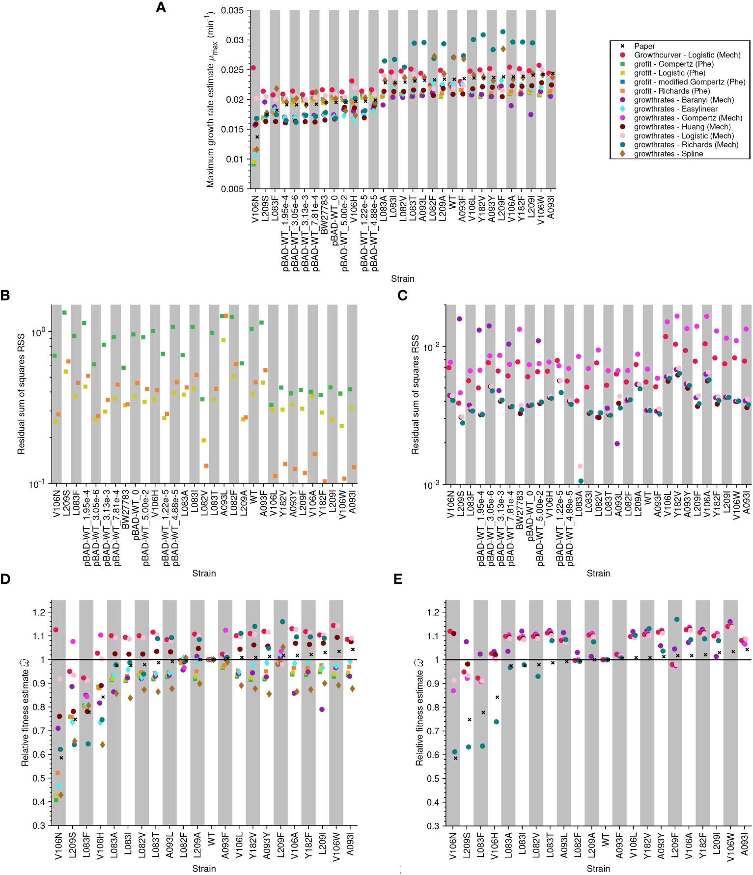
Figure 5 Analysis of published data-sets (Adkar et al., 2017) shows that estimates differ vastly depending on the method: (A) Maximum growth rate ${\widehat{\mu }}_{\max }$ estimate for each strain. Each growth curve was analyzed using three different R packages, including both model-free and model-based methods. The crosses show the values reported in the paper, the circles are obtained by methods based on mechanistic models, the squares by methods based on phenomenological models, and the diamonds by model-free methods. The model grofit - Logistic (Phe) describes a Logistic model with lag. (B) Goodness-of-fit measured as the residual sum of squares (RSS) by strain for the phenomenological models. (C) RSS by strain for the mechanistic models. We include the RSS of phenomenological and mechanistic models in different plots as the scale of the y-axes differs between these models: phenomenological models operate on a logarithmic scale since y = ln(N/N₀) but mechanistic models operate on a linear scale N(t). Relative fitness: (D, E) Relative fitness estimate $\widehat{\omega }$ versus strain. In (D), the relative fitness is computed using µ_max whereas in (E), it is computed using µ.

A visual inspection of the fits corroborates our findings that all models fit the data well (visualizations are available as part of the archived code repository on Zenodo 10.5281/zenodo.6629064). We emphasize that a visual inspection is important to ensure the estimated values are appropriate. Indeed, in a few cases, the fits proved unsatisfactory, although the summary statistics were good (see, e.g., Supplementary Figure S6).

No model is consistently preferred for all samples of a data set. This highlights the difficulty of choosing ‘the one’ right model, although this choice greatly impacts the growth parameter estimates. Whether phenomenological or mechanistic, the Gompertz equation frequently yielded the worst statistics, although our literature review indicated the phenomenological Gompertz equation as the most frequently used model. Moreover, the models used in the original data publications were not always the models we found to obtain the best statistics.

As previously stated, model-free methods may be preferred for some research questions, especially when neither the underlying mechanisms nor relative fitness estimates are of interest. Model-free methods obtain the maximum growth rate by determining the maximum of the function d ln(N(t)/N₀)/dt (see Figure 1C). A quick comparison with the derivative of the experimental data ensures the validity of the estimate. We found that Easy Linear gave slightly different results from the Spline method because the former requires the user to specify how many data points to include to analyze the log-linear part of the growth curve. Note that model-free methods are likely more accurate than model-based methods for estimating µ_max because the latter type involves more parameters and a data fit.

2.4.1 Relative growth rate estimates from empirical data

Adkar et al. (2017) used µ_max estimates from a phenomenological Gompertz model to estimate relative fitnesses. Therefore, this study allowed us to evaluate our concerns about using µ_max for relative fitness estimates. First, we used all approaches (model-free methods, phenomenological models, and mechanistic models) to estimate µ_max for the wild-type and mutant strains from this data set. Assuming (erroneously) that µ_max was a proxy for µ, we then calculated the relative fitness. Figure 5D shows that mechanistic models (circles) estimate more beneficial fitness values than methods that estimate µ_max directly (diamonds for model-free methods and squares for phenomenological models). Especially for strains estimated by Adkar et al., 2017 (crosses) to have especially low fitness, we found a large variation in the fitness values estimated by different methods.

Next, we used mechanistic models to estimate the intrinsic growth rate µ for the wild-type and mutant strains from this data set and subsequently calculated the relative fitness. In Figure 5E, we compared our estimated values with those published by Adkar et al. (2017). Again, many models estimate larger fitness values than those reported in the original study. This is especially pronounced for samples estimated by Adkar et al., 2017 (crosses) to have especially low fitness.

The overall conclusion of this section is that estimating relative fitness using inaccurate estimates of µ likely propagates to the level of relative fitness and causes large discrepancies between relative fitness values estimated using different methods. Importantly, these discrepancies are most pronounced for samples of special interest in an experiment.

2.4.2 Implications of data re-analysis

Our analysis indicates that choosing the best method to analyze growth curve data is very difficult. Identifying the ‘right’ model that best fits all strains/treatments within a data set seems daunting. This difficulty might explain why such a diversity of methods for analyzing growth curve data exists, as we found in the literature review. Interestingly, we saw that most articles only report using one data analysis method. We suspect that different labs and researchers have their preferences and habits on how to obtain growth rate estimates. In the interest of time (and sanity), researchers may be using the model and method they know best and for which they have obtained reasonable-looking results rather than trying out many unfamiliar computational tools.

One clear finding from our re-analysis of published data is that the Gompertz family of models – both phenomenological and mechanistic – are usually not the best choice. This point was previously made by López et al. (2004). We corroborate their empirical results with mathematical arguments. However, our literature review showed that the Gompertz models have remained popular long after López et al.’s study in 2004. We recommend that experimenters fit and compare more than one model when analyzing data. In light of our results, it will be important to develop one easy-to-use framework that allows for model choice and comparison, which would easily single out inappropriate models.

Our results confirmed the finding of (Peleg and Corradini, 2011) that standard statistical techniques for model selection were often unhelpful (Figures 5B, C): when comparing the fit of different models to the same data, the goodness-of-fit statistics did not always select the model that looked best upon visual inspection and/or there was not much difference between models in terms of goodness-of-fit. This corroborates our communications with empiricists that they are reluctant to use models for fitting their growth curve data.

3 Recommendations & conclusions

Despite the long-established study of batch culture growth curve data, estimating growth rates is still not straightforward. Using a literature review, math, simulations, and analysis of previously published data, our work highlights experimental and theoretical pitfalls encountered by many researchers who work with batch monoculture growth curves. We have summarized our recommendations for better growth rate estimates as a checklist in Figure 6.

Figure 6

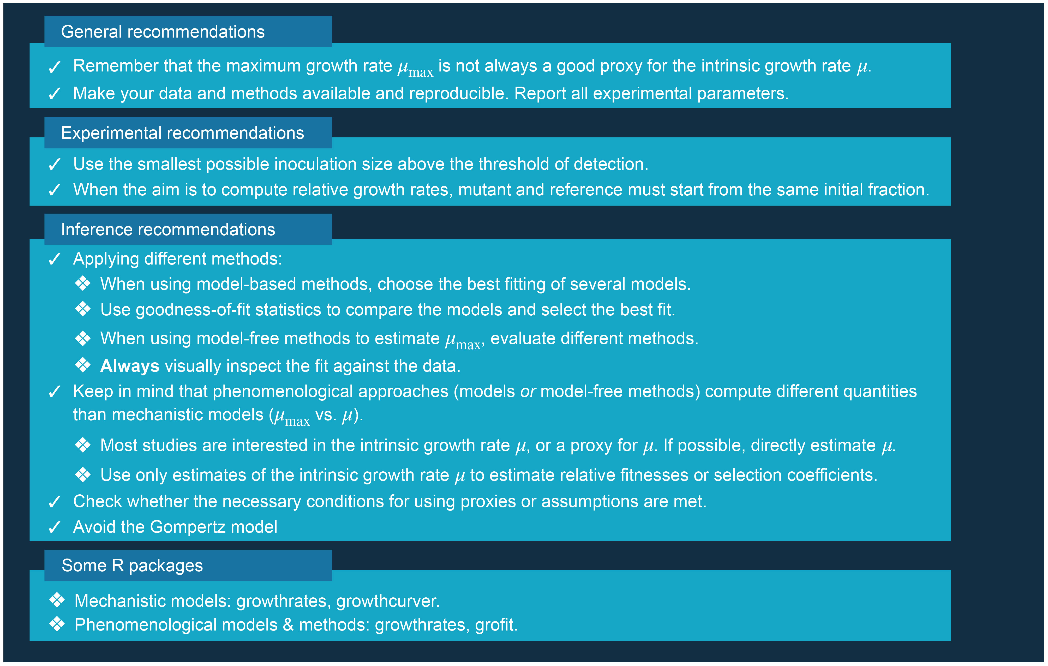
Figure 6 A list of recommendations for better growth rate inference from monoculture growth curves.

3.1 General recommendations

We urge readers to remember that the intrinsic growth rate µ, a model parameter estimated from mechanistic models, is not the same as the maximum growth rate µ_max, a summary-statistic estimated using phenomenological models or by model-free methods. Although µ_max is often used as a proxy for µ, this assumption is not always justified. In particular, this assumption can only be justified when small and equal initial population fractions of the mutant and wild-type strains are used and if the strains do not exhibit a lag phase.

We recommend that researchers make their raw data and methods available and reproducible. In particular, this involves reporting all experimental parameters like inoculum size (for experiments with a fixed N₀) or carrying capacity/density of the inoculating-culture and the dilution factor (for experiments with a fixed dilution fraction), and lag time. During our literature review, we were surprised by the lack of sufficient information on experimental methods, estimated values, and data availability.

3.2 Experimental recommendations

Good data begins with good experimental methods. In the absence of a lag phase, the fastest growth rate (both for the maximum growth rate µ_max and for the intrinsic growth rate µ) is observed at the very start of the growth curve. As we show in Figures 3A and 4, estimates of interest can be highly sensitive to the inoculum size. Also, when a lag phase is suspected, reliable data from the start of the growth curve is necessary to quantify the lag time and growth rate. Therefore, we recommend that experimenters use the smallest inoculation size possible that is still reliably above the detection threshold. If cell counts are to be approximated using optical density, then it is imperative that the data be appropriately calibrated following the recommendations of Hall et al., 2014; Stevenson et al., 2016; Mira et al., 2022.

For accurate estimation of the relative growth rate, we stress that the mutant and reference/wild-type strains should start from the same initial population fraction ( $N_0^M/K_M=N_0^{WT}/K_{WT}$; Figure 4), which is not necessarily the same absolute size. Suppose the strains have the same carrying capacity (K_M = K_WT) at the stationary phase. In that case, it is possible to either dilute the cultures used for inoculation by the same dilution factor or begin the growth curves at the same absolute inoculum size ( $N_0^M=N_0^{WT}$). However, if the carrying capacities differ between strains, then the same absolute inoculum size cannot be used. We found in our literature review that about half of the papers use a fixed absolute inoculum size to start their growth curve experiments. In contrast, the other half uses a fixed dilution factor, usually without justifying either choice. We recommend that experimenters interested in calculating relative growth rates use a fixed dilution factor. A pilot experiment is ideal for predicting the carrying capacities and corresponding optimal inoculum sizes.

By following these recommendations, monoculture growth curves can be used to predict relative growth rate/fitness and to better understand interactions between strains/species. Estimated growth rates from monocultures can be used to generate a priori predictions for the outcome of a direct competition (for example, using mechanistic consumer resource models). Comparison of the predicted outcome and the observed outcome of competition can distinguish between interactions due to differences in growth rates alone as compared to the presence of direct interactions (reviewed in Picot et al., 2023).

3.3 Inference recommendations

Regarding inference methods, our main recommendation is to try out several different methods on the same data. We recommend that a computational method be used to estimate the growth rate. (Manual) Fitting of an exponential model should be avoided (Table 3), regardless of whether the exponential model is fit explicitly or implicitly by using the equation R =(log₂ N₂ − log₂ N₁)/(t₂ − t₁).

Model-free computational methods tend to be technically easier to use than model-based methods, but they can only estimate µ_max. Model-based methods often require more computational knowledge for fitting, but we still recommend that researchers try to fit more than one model. For those familiar with the R statistical programming language, we recommend the growthrates package because all of the mechanistic models presented in Table 1, as well as model-free methods for estimating µ_max, can easily be fitted with this package. We recommend that researchers use goodness-of-fit summary statistics (like the RSS, AIC, etc.) to compare models and select the best fit. Additional visual inspection of the estimated value and the data is essential because goodness-of-fit statistics can be misleading (e.g., Supplementary Figure S6).

Our work explains and demonstrates that and why the maximum growth rate µ_max is different from the intrinsic growth rate µ, which is a key point to take away and remember from this paper. We suggest that researchers attempt to estimate µ directly from their data using mechanistic models. However, we have shown that using the phenomenological quantity µ_max as a proxy for the model parameter µ can be justified, if certain conditions are met. We recommend that experimenters decide which makes more sense for the experimental question at hand and, based on that decision, select the types of models or model-free approaches to use. If µ_max is to be inferred, model-free methods or fits of phenomenological models can be used. Model-based methods can either be used to estimate the maximum growth rate µ_max of phenomenological models or the intrinsic growth rate µ of mechanistic models. We urge experimenters to refrain from comparing estimates obtained from mechanistic and phenomenological models because these different model types estimate different growth rate parameters. Researchers should know that confusion between the two quantities is common and that different authors/fields use different naming conventions. We hope this paper provides readers with the necessary conceptual understanding to navigate the literature critically. Finally, we note that only the intrinsic growth rate µ (and not µ_max or the exponential approximation) should be used for estimating the relative fitness (Figure 4) from monoculture growth curves.

It is important to verify that the necessary conditions are met for the inference method(s) to be used. For example, the exponential approximation should only be used when the inoculum size is much smaller than the carrying capacity ($N_0\ll K$, e.g., by at least 2 orders of magnitude), only time points at which the population size remains much smaller than the carrying capacity are considered ($N(t)\ll K$), and the lag time is very short or absent (e.g., $h_0\ll 1$ for growth following a Baranyi model). Given these restrictive assumptions, rather than demonstrating that the conditions for the exponential approximation are met, it may be more feasible for researchers to directly fit one of the mechanistic models listed in Table 1. Another approximation that requires justification is the use of µ_max as a proxy for µ. This approximation is only valid for small initial population fractions (Figure 3) and short (or absent) lag times. To demonstrate that this is the case, it is essential that experimenters report the initial population fraction(s) and the lag time(s) when using µ_max as a proxy for µ.

Finally, we recommend that researchers avoid fitting the Gompertz model for both absolute and relative estimates of µ. In our study, the mechanistic Gompertz model consistently showed wrong estimates for simulated data (Figures 3, 4) and unusually large estimates for empirical data (Figure 5).

4 Methods

4.1 Literature review

We quantified the most frequently used methods of analyzing growth curve data for extracting summary statistics. In July-September 2021, we queried Web of Knowledge and Google Scholar for papers from 1990-2021 using the following search terms: “Bioscreen C”, “growth curve”, “OD”, “optical density”, “growth rate”, “batch culture”, or “bacterial OR microbial”. Two papers (Gullberg et al., 2011; Trindade et al., 2012) were selected using the former criteria. However, these search terms proved too vague to yield useful results. Instead, most papers were found because they cited one of the following growth curve methods papers, Zwietering et al. (1990); Hall et al. (2014); Sprouffske and Wagner (2016); or Delaney et al. (2013). The total citations to these papers were filtered to include only those published in journals related to evolution, ecology, or evolutionary/ecological microbiology. The resultant 262 publications were considered for inclusion in the literature review if they gathered any type of growth curve data proportional to the number of individuals growing in a homogeneous, liquid culture and estimated growth parameters from that data. Papers that quantified binary presence/absence of growth (e.g., to assay lag time or spore viability), quantified only the areaunder-the curve (AUC), or investigated biofilms were excluded. A sample of 48 papers was selected using the latter criteria. From each paper, we extracted information about whether the method used to analyze growth curves is explicitly cited or described, what type(s) of growth curve summary statistic was used, whether a model-free or model-based approach was used, whether the growth rate is from a phenomenological or mechanistic approach, which model(s) were fitted (if no equation is given, then the name of the model as reported by the author), whether the growth curves were inoculated from a fixed starting value or the inoculating-culture was diluted by a fixed dilution factor, and whether the growth curve raw data is publicly available or, at least, plotted (summarized in Table S1). For papers where growth curves were inoculated using a dilution of the inoculating-culture, the dilution factor itself was used as an estimator of the dilution fraction. If given, we extracted the initial dilution factor and any accompanying information about the inoculum (e.g., length of overnight culture) to indicate whether the dilution factor is a good proxy for the initial population fraction (N₀/K). For papers where growth curves were inoculated using a fixed absolute initial population size, we estimated the dilution fraction only if sufficient information about the inoculum size and carrying capacity was provided in the methods. Finally, we categorized different model-free growth rate estimation methods that were applied ad hoc as either “Easy Linear” if a consistent method was given for selecting which points to include in the regression (since this is the main feature of popular model-free methods like that of Hall et al., 2014), or as “exponential approximation” if there was no information about which points were included in the regression or as “spline” if pairs of successive measurements were used to estimate the local slope of the curve.

4.2 Analyzing 4 published data sets

Data sets appropriate for our analysis were found during our literature review, and the data was accessed as indicated in each paper.

We used the following R (version 4.1.1) packages to re-analyze the data: Growthcurver (version 0.3.1), grofit (version 1.1.1-1), and growthrates (version 0.8.2). Each of them was downloaded from the CRAN repository except grofit, which we obtained from Kahm et al. (2010). Indeed, the latter was found to have been removed from the CRAN repository. The package Growthcurver is based on the mechanistic logistic model, whereas grofit includes four phenomenological models (Logistic, Gompertz, modified Gompertz, and Richards). The package growthrates provides both model-free methods (Easy Linear and Spline) as well as methods based on mechanistic models (Logistic, Gompertz, Richards, Baranyi, and Huang).

We analyzed 143 population growth curves (31 from Adkar et al., 2017; 6 from Ram et al., 2019; 66 from Todd and Selmecki, 2020; and 40 from Hammer et al., 2021) using all methods mentioned above. We focused on the maximum growth rate µ_max, because it is the only quantity common to all models and methods. Since the mechanistic models are defined based on the intrinsic growth rate µ, we used Table 1 to calculate the maximum growth rate µ_max from the respective model.

To test the accuracy of the fits obtained by the model-based methods, we calculated the residual sum of squares (RSS). We used the definition from López et al. (2004):

$$\text{RSS }={\displaystyle \sum _{i=1}^n{(O{D}_i-\widehat{O{D}_i})}^2.}$$

Here, n is the number of data points, OD_i is the i^th optical density value to be estimated and $\widehat{O{D}_i}$ is the i^th estimated optical density value. Since the models have different numbers of parameters, we also calculated the Akaike’s Information Criterion (AIC) for the mechanistic models as given in López et al. (2004) and explained in the Supplementary Methods.

4.3 Simulations

We generated data representing the dynamics of microbial populations using a Gillespie algorithm for the mechanistic Gompertz, Richards and Logistic models (Gillespie, 1976; Gillespie, 1977). For the Baranyi and Huang models, a modified Next-Reaction algorithm was required since these models have time-dependent growth rates (Anderson, 2007). All simulation code was written in C and is available at https://github.com/LcMrc/GrowthRates (Zenodo 10.5281/zenodo.6629064). We detail below the algorithms used.

Gillespie algorithm: Let us denote by N the number of individuals. The only elementary event that can happen is division of a microbe, whose rate is denoted by k_N→N+1. Let us note that k_N→N+1 = µ log(K/N)N, k_N→N+1 = µ(1 − N/K)N and k_N→N+1 = µ(1 − (N/K)^β)N for the mechanistic Gompertz, Logistic and Richards models, respectively. Simulation steps are as follows:

1. Initialization: The population starts from N₀ microorganisms at time t = 0.

2. Time update: The time increment Δt is sampled randomly from an exponential distribution with mean 1/k_N→N+1 and the time t is updated such that t ← t + Δt.

3. Number of individuals update: a division occurs and the population size N increases by one such that N ← N + 1.

4. We go back to Step 2 and iterate until the desired time limit is reached.

Next-Reaction algorithm: Let us denote by N the number of individuals. The only elementary event that can happen is division of a microbe, whose time-dependent rate is denoted by k_N→N+1(t). Let us note that k_N→N+1(t) = µe^µt(1 − N/K)N/(e^h0 − 1 + e^µt) and k_N→N+1(t) = µ(1 − N/K)N/(1 + e^α(t−τ)) for the mechanistic Baranyi and Huang models, respectively. In the following, we will denote by P the first firing time and T the internal time.

1. initialization: The population starts from N₀ microorganisms at time t = 0. The first firing time P is sampled from an exponential distribution of mean 1 and the internal time T is set to 0.

2. Time update: The time increment Δt is computed solving ${\displaystyle {\int }_t^{t+\Delta t}{k}_{N\to N+1}(u)\text{d}u=P-T}$ and the time t is updated such that t ← t + Δt.

3. Number of individuals update: a division occurs and the population size N increases by one such that N ← N + 1.

4. Internal time update: The internal time T is updated such that T ← T + ΔT, where $\Delta T={\displaystyle {\int }_t^{t+\Delta t}{k}_{N\to N+1}(u)\text{d}u.}$

5. First firing time update: The first firing time P is updated such that P ← P + ΔP, where ΔP is sampled from an exponential distribution of mean 1.

6. We go back to Step 2 and iterate until the desired time limit is reached.

4.4 Data availability

The authors state that all data necessary for confirming the conclusions presented in the article are represented fully within the article or Supplemental Material. Annotated C implementations of numerical simulations, annotated code to reproduce all computationally produced graphs, and additional figures and tables reporting the data re-analysis fits and estimates are available on Zenodo 10.5281/zenodo.6629064.

Data availability statement

The original contributions presented in the study are included in the article/Supplementary Files. Further inquiries can be directed to the corresponding authors.

Author contributions

LM: Conceptualization, Data curation, Formal analysis, Investigation, Methodology, Project administration, Resources, Software, Validation, Visualization, Writing – original draft, Writing – review & editing. A-HG: Conceptualization, Data curation, Formal analysis, Funding acquisition, Investigation, Methodology, Project administration, Resources, Software, Validation, Visualization, Writing – original draft, Writing – review & editing. CB: Conceptualization, Funding acquisition, Project administration, Supervision, Writing – review & editing.

Funding

The author(s) declare financial support was received for the research, authorship, and/or publication of this article. A-HG thanks FCT PhD funding grant PD/BD/138215/2018. CB is grateful for funding from ERC Starting Grant 804569 (FIT2GO) and SNSF Project Grant “MiCo4Sys”.

Acknowledgments

The authors thank the Evolutionary Biology group at IGC for stimulating discussions and the THEE Group at UniBe for feedback on the manuscript.

Conflict of interest

The authors declare that the research was conducted in the absence of any commercial or financial relationships that could be construed as a potential conflict of interest.

Publisher’s note

All claims expressed in this article are solely those of the authors and do not necessarily represent those of their affiliated organizations, or those of the publisher, the editors and the reviewers. Any product that may be evaluated in this article, or claim that may be made by its manufacturer, is not guaranteed or endorsed by the publisher.

Supplementary material

The Supplementary Material for this article can be found online at: https://www.frontiersin.org/articles/10.3389/fevo.2023.1313500/full#supplementary-material

Glossary

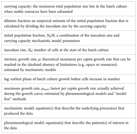
References

Adkar B. V., Manhart M., Bhattacharyya S., Tian J., Musharbash M., Shakhnovich E. I. (2017). Optimization of lag phase shapes the evolution of a bacterial enzyme. Nat. Ecol. Evol. 1 (6), 149. doi: 10.1038/s41559-017-0149

PubMed Abstract | CrossRef Full Text | Google Scholar

Anderson D. F. (2007). A modified next reaction method for simulating chemical systems with time dependent propensities and delays. J. Chem. Phys. 127 (21), 214107. doi: 10.1063/1.2799998

PubMed Abstract | CrossRef Full Text | Google Scholar

Ashino K., Sugano K., Amagasa T., Ying B.-W. (2019). Predicting the decision making chemicals used for bacterial growth. Sci. Rep. 9, 7251. doi: 10.1038/s41598-019-43587-8

PubMed Abstract | CrossRef Full Text | Google Scholar

Baranyi J., Roberts T. A. (1994). A dynamic approach to predicting bacterial growth in food. Int. J. Food Microbiol. 23 (3), 277–294. doi: 10.1016/0168-1605(94)90157-0

PubMed Abstract | CrossRef Full Text | Google Scholar

Baranyi J., Roberts T. A. (1995). Mathematics of predictive food microbiology. Int. J. Food Microbiol. 26 (2), 199–218. doi: 10.1016/0168-1605(94)00121-L

PubMed Abstract | CrossRef Full Text | Google Scholar

Basra P., Alsaadi A., Bernal-Astrain G., O’Sullivan M. L., Hazlett B., Clarke L. M., et al. (2018). Fitness tradeoffs of antibiotic resistance in extraintestinal pathogenic Escherichia coli. Genome Biol. Evol. 10 (2), 667–679. doi: 10.1093/gbe/evy030

PubMed Abstract | CrossRef Full Text | Google Scholar

Bernhardt J. R., Kratina P., Pereira A. L., Tamminen M., Thomas M. K., Narwani A. (2020). The evolution of competitive ability for essential resources. Philos. Trans. R. Soc. B 375 (1798), 20190247. doi: 10.1098/rstb.2019.0247

CrossRef Full Text | Google Scholar

Blomberg A. (2011). Measuring growth rate in high-throughput growth phenotyping. Curr. Opin. Biotechnol. 22 (1), 94–102. doi: 10.1016/j.copbio.2010.10.013

PubMed Abstract | CrossRef Full Text | Google Scholar

Bolker B. M. (2008). Ecological models and data in R. (Princeton, New Jersey, USA: Princeton University Press).

Google Scholar

Carlson T. (1913). Übergeschwindigkeit und grösse der hefevermehrung in würze. Biochem. Ztschr. Bd. 57, 313–334.

Google Scholar

Chevin L.-M. (2011). On measuring selection in experimental evolution. Biol. Lett. 7 (2), 210–213. doi: 10.1098/rsbl.2010.0580

PubMed Abstract | CrossRef Full Text | Google Scholar

Chezeau B., Vial C. (2019). Modeling and simulation of the biohydrogen production processes Vol. 19 (Amsterdam, Netherlands: Elsevier B.V. All), 445–483. doi: 10.1016/C2017-0-03531-

CrossRef Full Text | Google Scholar

Concepci´on-Acevedo J., Weiss H. N., Chaudhry W. N., Levin B. R. (2015). Malthusian parameters as estimators of the fitness of microbes: a cautionary tale about the low side of high throughput. PloS One 10 (6), e0126915. doi: 10.1371/journal.pone.0126915

PubMed Abstract | CrossRef Full Text | Google Scholar

Crow J. F., Kimura M. (2009). An introduction to population genetics theory. (Caldwell, New Jersey, USA: Blackburn Press). Available at: https://books.google.pn/books?id=VWqKPwAACAAJ, ISBN: 9781932846126.

Google Scholar

Delaney N. (2014) Curve Fitter - software for growth curve fitting and visualization. Available at: http://www.evolvedmicrobe.com/CurveFitter/ (Accessed 2021-11-23).

Google Scholar

Delaney N. F., Kaczmarek M. E., Ward L. M., Swanson P. K., Lee M.-C., Marx C. J. (2013). Development of an optimized medium, strain and high-throughput culturing methods for Methylobacterium extorquens. PloS One 8 (4), e62957. doi: 10.1371/journal.pone.0062957

PubMed Abstract | CrossRef Full Text | Google Scholar

Fernandez-Ricaud L., Kourtchenko O., Zackrisson M., Warringer J., Blomberg A. (2016). Precog: a tool for automated extraction and visualization of fitness components in microbial growth phenomics. BMC Bioinf. 17 (1), 1–15. doi: 10.1186/s12859-016-1134-2

CrossRef Full Text | Google Scholar

Ganucci D., Guerrini S., Mangani S., Vincenzini M., Granchi L. (2018). Quantifying the effects of ethanol and temperature on the fitness advantage of predominant Saccharomyces cerevisiae strains occurring in spontaneous wine fermentations. Front. Microbiol. 9, 1563. doi: 10.3389/fmicb.2018.01563

PubMed Abstract | CrossRef Full Text | Google Scholar

Gillespie D. T. (1976). A general method for numerically simulating the stochastic time evolution of coupled chemical reactions. J. Comput. Phys. 22 (4), 403–434. doi: 10.1016/0021-9991(76)90041-3

CrossRef Full Text | Google Scholar

Gillespie D. T. (1977). Exact stochastic simulation of coupled chemical reactions. J. Phys. Chem. 81 (25), 2340–2361. doi: 10.1021/j100540a008

CrossRef Full Text | Google Scholar

Gullberg E., Cao S., Berg O. G., Ilbäck C., Sandegren L., Hughes D., et al. (2011). Selection of resistant bacteria at very low antibiotic concentrations. PloS Pathog. 7 (7), e1002158. doi: 10.1371/journal.ppat.1002158

PubMed Abstract | CrossRef Full Text | Google Scholar

Hall B. G., Acar H., Nandipati A., Barlow M. (2014). Growth rates made easy. Mol. Biol. Evol. 31 (1), 232–238. doi: 10.1093/molbev/mst187

PubMed Abstract | CrossRef Full Text | Google Scholar

Hammer T. J., Le E., Moran N. A. (2021). Thermal niches of specialized gut symbionts: the case of social bees. Proc. R. Soc. B: Biol. Sci. 288 (1944), 20201480. doi: 10.1098/rspb.2020.1480

CrossRef Full Text | Google Scholar

Huang L. (2011). A new mechanistic growth model for simultaneous determination of lag phase duration and exponential growth rate and a new bĕlehdrádek-type model for evaluating the effect of temperature on growth rate. Food Microbiol. 28 (4), 770–776. doi: 10.1016/j.fm.2010.05.019

PubMed Abstract | CrossRef Full Text | Google Scholar

Jung P. P., Christian N., Kay D. P., Skupin A., Linster C. L. (2015). Protocols and programs for high-throughput growth and aging phenotyping in yeast. PloS One 10 (3), e0119807. doi: 10.1371/journal.pone.0119807

PubMed Abstract | CrossRef Full Text | Google Scholar

Kahm M., Hasenbrink G., Lichtenberg-Frat´e H., Ludwig J., Kschischo M. (2010). grofit: Fitting biological growth curves with R. J. Stat. Software 33 (7), 1–21. doi: 10.18637/jss.v033.i07

CrossRef Full Text | Google Scholar

Kassen R. (2014) Experimental evolution and the nature of biodiversity. Macmillan learning. Available at: https://books.google.ch/books?id=LL8YnwEACAAJ.

Google Scholar

Khan S., Beattie T. K., Knapp C. W. (2017). The use of minimum selectable concentrations (MSCs) for determining the selection of antimicrobial resistant bacteria. Ecotoxicology 26 (2), 283–292. doi: 10.1007/s10646-017-1762-y

PubMed Abstract | CrossRef Full Text | Google Scholar

Knopp M., Andersson D. I. (2018). Predictable phenotypes of antibiotic resistance mutations. MBio 9 (3), e00770–18. doi: 10.1128/mBio.00770-18

PubMed Abstract | CrossRef Full Text | Google Scholar

Krishnamurthi V. R., Niyonshuti I. I., Chen J., Wang Y. (2021). A new analysis method for evaluating bacterial growth with microplate readers. PloS One 16 (1), e0245205. doi: 10.1371/journal.pone.0245205

PubMed Abstract | CrossRef Full Text | Google Scholar

Kurokawa M., Ying B.-W. (2017). Precise, high-throughput analysis of bacterial growth. J. Visualized Experiments: JoVE 127, e56197. doi: 10.3791/56197

CrossRef Full Text | Google Scholar

Lenski R. E., Rose M. R., Simpson S. C., Tadler S. C. (1991). Longterm experimental evolution in escherichia coli. i. adaptation and divergence during 2,000 generations. Am. Nat. 138 (6), 1315–1341. doi: 10.1086/285289

CrossRef Full Text | Google Scholar

Liberles D. A., Teufel A. I., Liu L., Stadler T. (2013). On the need for mechanistic models in computational genomics and metagenomics. Genome Biol. Evol. 5 (10), 2008–2018. doi: 10.1093/gbe/evt151

PubMed Abstract | CrossRef Full Text | Google Scholar

López S., Prieto M., Dijkstra J., Dhanoa M. S., France J. (2004). Statistical evaluation of mathematical models for microbial growth. Int. J. Food Microbiol. 96 (3), 289–300. doi: 10.1016/j.ijfoodmicro.2004.03.026

PubMed Abstract | CrossRef Full Text | Google Scholar

Mallet J. (2012). The struggle for existence. how the notion of carrying capacity, k, obscures the links between demography, darwinian evolution and speciation. Evolutionary Ecol. Res. 14, 627–665.

Google Scholar

Midani F. S., Collins J., Britton R. A. (2021). Amiga: software for automated analysis of microbial growth assays. Msystems 6 (4), e00508–21. doi: 10.1128/mSystems.00508-21

PubMed Abstract | CrossRef Full Text | Google Scholar

Miller T. E., Burns J. H., Munguia P., Walters E. L., Kneitel J. M., Richards P. M., et al. (2005). A critical review of twenty years’ use of the resource-ratio theory. Am. Nat. 165 (4), 439–448. doi: 10.1086/428681

PubMed Abstract | CrossRef Full Text | Google Scholar

Mira P., Barlow M., Meza J. C., Hall B. G. (2017). Statistical package for growth rates made easy. Mol. Biol. Evol. 34 (12), 3303–3309. doi: 10.1093/molbev/msx255

PubMed Abstract | CrossRef Full Text | Google Scholar

Mira P., Yeh P., Hall B. G. (2022). Estimating microbial population data from optical density. PloS One 17 (10), e0276040. doi: 10.1371/journal.pone.0276040

PubMed Abstract | CrossRef Full Text | Google Scholar

Monod J. (1949). The growth of bacterial cultures. Annu. Rev. Microbiol. 3 (1), 371–394. doi: 10.1146/annurev.mi.03.100149.002103

CrossRef Full Text | Google Scholar

Munafò M. R., Nosek B. A., Bishop D. V. M., Button K. S., Chambers C. D., du Sert N. P., et al. (2017). A manifesto for reproducible science. Nat. Hum. Behav. 1 (1), 1–9. doi: 10.1038/s41562-016-0021

CrossRef Full Text | Google Scholar

Novak M., Pfeiffer T., Ackermann M., Bonhoeffer S. (2009). Bacterial growth properties at low optical densities. Antonie Van Leeuwenhoek 96 (3), 267–274. doi: 10.1007/s10482-009-9342-7

PubMed Abstract | CrossRef Full Text | Google Scholar

Otto S. P., Day T. (2011). A biologist’s guide to mathematical modeling in ecology and evolution. (Princeton, New Jersey, USA: Princeton University Press).

Google Scholar

Peleg M., Corradini M. G. (2011). Microbial growth curves: what the models tell us and what they cannot. Crit. Rev. Food Sci. Nutr. 51 (10), 917–945. doi: 10.1080/10408398.2011.570463

PubMed Abstract | CrossRef Full Text | Google Scholar

Perni S., Andrew P. W., Shama G. (2005). Estimating the maximum growth rate from microbial growth curves: definition is everything. Food Microbiol. 22 (6), 491–495. doi: 10.1016/j.fm.2004.11.014

CrossRef Full Text | Google Scholar

Petzoldt T. (2020) growthrates: estimate growth rates from experimental data. Available at: https://CRAN.R-project.org/package=growthrates.

Google Scholar

Picot A., Shibasaki S., Meacock O. J., Mitri S. (2023). Microbial interactions in theory and practice: when are measurements compatible with models? Curr. Opin. Microbiol. 75, 102354. doi: 10.1016/j.mib.2023.102354

PubMed Abstract | CrossRef Full Text | Google Scholar

Ram Y., Dellus-Gur E., Bibi M., Karkare K., Obolski U., Feldman M. W., et al. (2019). Predicting microbial growth in a mixed culture from growth curve data. Proc. Natl. Acad. Sci. 116 (29), 14698–14707. doi: 10.1073/pnas.1902217116

CrossRef Full Text | Google Scholar

Rodrigue N., Philippe H. (2010). Mechanistic revisions of phenomenological modeling strategies in molecular evolution. Trends Genet. 26 (6), 248–252. doi: 10.1016/j.tig.2010.04.001

PubMed Abstract | CrossRef Full Text | Google Scholar

Slator A. (1916). Ii. the rate of growth of bacteria. J. Chem. Soc. Trans. 109, 2–10. doi: 10.1039/CT9160900002

CrossRef Full Text | Google Scholar

Sprouffske K., Wagner A. (2016). Growthcurver: an R package for obtaining interpretable metrics from microbial growth curves. BMC Bioinf. 17 (1), 172, 4. doi: 10.1186/s12859-016-1016-7

CrossRef Full Text | Google Scholar

Stevenson K., McVey A. F., Clark I. B. N., Swain P. S., Pilizota T. (2016). General calibration of microbial growth in microplate readers. Sci. Rep. 6 (1), 1–7. doi: 10.1038/srep38828

PubMed Abstract | CrossRef Full Text | Google Scholar

Todd R. T., Selmecki A. (2020). Expandable and reversible copy number amplification drives rapid adaptation to antifungal drugs. eLife 9, e58349. doi: 10.7554/eLife.58349

PubMed Abstract | CrossRef Full Text | Google Scholar

Trindade S., Sousa A., Gordo I. (2012). Antibiotic resistance and stress in the light of fisher’s model. Evolution 66 (12), 3815–3824. doi: 10.1111/j.1558-5646.2012.01722.x

PubMed Abstract | CrossRef Full Text | Google Scholar

Tsoularis A., Wallace J. (2002). Analysis of logistic growth models. Math. Biosci. 179 (1), 21–55. doi: 10.1016/S0025-5564(02)00096-2

PubMed Abstract | CrossRef Full Text | Google Scholar

Wahl L. M., Zhu A. D. (2015). Survival probability of beneficial mutations in bacterial batch culture. Genetics 200 (1), 309–320. doi: 10.1534/genetics.114.172890

PubMed Abstract | CrossRef Full Text | Google Scholar

Wein T., Dagan T. (2019). The effect of population bottleneck size and selective regime on genetic diversity and evolvability in bacteria. Genome Biol. Evol. 11 (11), 3283–3290. doi: 10.1093/gbe/evz243

PubMed Abstract | CrossRef Full Text | Google Scholar

Wilkinson M. D., Dumontier M., Aalbersberg I. J., Appleton G., Axton M., Baak A., et al. (2016). The FAIR guiding principles for scientific data management and stewardship. Sci. Data 3 (1), 1–9. doi: 10.1038/sdata.2016.18

CrossRef Full Text | Google Scholar

Wu X., Jacobs N. T., Bozio C., Palm P., Lattar S. M., Hanke C. R., et al. (2017). Competitive dominance within biofilm consortia regulates the relative distribution of pneumococcal nasopharyngeal density. Appl. Environ. Microbiol. 83 (16), e00953–e00917. doi: 10.1128/AEM.00953-17

PubMed Abstract | CrossRef Full Text | Google Scholar

Yang R.-J., Wang X.-L., Zhang Y.-Y., Zhan Y.-J. (2006). Influence of cell equivalent spherical diameter on the growth rate and cell density of marine phytoplankton. J. Exp. Mar. Biol. Ecol. 331 (1), 33–40. doi: 10.1016/j.jembe.2005.09.015

CrossRef Full Text | Google Scholar

Zwietering M. H., Jongenburger I., Rombouts F. M., Van’t Riet K. (1990). Modeling of the bacterial growth curve. Appl. Environ. Microbiol. 56 (6), 1875–1881. doi: 10.1128/aem.56.6.1875-1881.1990

PubMed Abstract | CrossRef Full Text | Google Scholar