Latitudinal diversity of planktonic copepods in the Eastern Pacific: overcoming sampling biases and predicting patterns

Introduction

The latitudinal diversity gradient (LDG) is one of the most striking features in ecology and biogeography. Contrary to the classic notion of an increase in diversity from the poles towards the equator (Rohde, 1992), studies in marine systems have shown that diversity is higher at mid-latitudes and decreases towards the equator (Rombouts et al., 2009; Barton et al., 2010; Chaudhary et al., 2016; Saeedi et al., 2017; Rivadeneira and Poore, 2020; Lin et al., 2021), which constitutes a pattern that has remained constant for millions of years (Yasuhara et al., 2012).

Over a large latitudinal gradient, the highest diversity of marine organisms has been reported in subtropical areas of the Northern Hemisphere, and a tropical-subtropical plateau in the Southern Hemisphere (Rutherford et al., 1999; Rombouts et al., 2009; Fautin et al., 2013; Chaudhary et al., 2016; O’Brien et al., 2016; Saeedi et al., 2017; Saeedi et al., 2019b; Rivadeneira and Poore, 2020; Chaudhary et al., 2021; Lin et al., 2021), together with a decrease in species richness near the equator (Chaudhary et al., 2016; Menegotto and Rangel, 2018). Although this pattern has been attributed to sampling biases (Menegotto and Rangel, 2018), empirical evidence supports this latitudinal trend (e.g., Chaudhary et al., 2016, 2017; Saeedi et al., 2017; Chaudhary and Costello, 2023, 2019b), reported for mollusks (Saeedi et al., 2017, 2019b), foraminifera (Brayard et al., 2005), coccolithophores (O’Brien et al., 2016), ophiuroids (Woolley et al., 2016), crustaceans (Rivadeneira and Poore, 2020), polychaete worms (Pamungkas and Glasby, 2021), brown macroalgae (Fragkopoulou et al., 2022), and higher trophic level organisms, such as fishes, sharks, squids, and cetaceans (Rutherford et al., 1999; Tittensor et al., 2010). This spatial pattern among taxonomically distant species suggests the existence of a common underlying mechanism that supports their similar distributions (Worm et al., 2005; Rombouts et al., 2011), which has been mainly attributed to the energy or temperature hypothesis (Hawkins et al., 2003; Rombouts et al., 2011).

The geographic patterns of diversity in marine environments have long been described (see Tittensor et al., 2010; Beaugrand et al., 2013; Miller et al., 2018); however, the ecological and evolutionary mechanisms of these patterns are not well understood (Roy et al., 1998; Gagné et al., 2020; Melo-Merino et al., 2020; Moreno et al., 2021). Most hypotheses attempting to explain contemporary patterns of diversity are based on the link between the abiotic environment and species diversity (Pianka, 1966; Currie, 1991; Rutherford et al., 1999; Kerr, 2001). Nevertheless, there is a lack of consensus regarding the mechanisms that cause such relationships (Stokes, 2018). Indeed, a particular set of environmental ecological hypotheses (e.g., energy, productivity, and environmental heterogeneity) has been suggested to explain the processes underlying the distribution of diversity in the oceans (e.g., Tittensor et al., 2010; Worm and Tittensor, 2018; Brandão et al., 2021). Among these factors, temperature and productivity may exhibit the highest explanatory power (Rutherford et al., 1999; Tittensor et al., 2010). Thus, they have been proposed as the main driver of diversity in multiple marine taxa (Irigoien et al., 2004; Brayard et al., 2005; Tittensor et al., 2010; Saeedi et al., 2019a; Lin et al., 2021).

In the same context, studies on planktonic copepods’ diversity and geographic variability in relation to environmental parameters have been performed (Rutherford et al., 1999; Rombouts et al., 2009, 2011; Hooff and Peterson, 2006; Medellín-Mora et al., 2016; González et al., 2020), showing a strong temperature dependence, resulting from the effect of this variable on the vital rates and ecological responses of copepods. Nevertheless, despite their ecological importance and the relatively high amount of data available on their distribution, open ocean studies on their biogeographic patterns are scarce and underrepresented in global biodiversity assessments, with studies mostly concentrated on local systems of the Pacific (e.g., Williamson and McGowan, 2010; Medellín-Mora et al., 2016; González et al., 2020, 2021). Furthermore, the mechanisms or factors that explain and modulate diversity on a wide scale are insufficiently understood, and too few studies have been conducted using explicit spatial analysis to understand and predict biogeographic patterns (Wilson et al., 2016; Brandão et al., 2021; Rivera et al., 2023).

When studying biogeographic patterns, the total diversity in a region (gamma diversity) can be decomposed into alpha and beta diversity. Alpha diversity refers to diversity within a local community, whereas beta diversity refers to variability between different communities or sites. It is relevant to note that the factors underlying alpha, or beta diversity are different (Leprieur et al., 2011), including historical and environmental processes. Therefore, it is important to explicitly know the factors that modulate the spatial structure of copepods along broad environmental gradients when evaluating ecological hypotheses (e.g., energy, heterogeneity, productivity) that would explain these diversity trends.

Beta-diversity is a less studied attribute of copepod diversity over a broad geographic scale. Beta diversity represents the extent of change in community composition or the degree of community differentiation in relation to environmental gradients (Whittaker, 1960). The importance of beta diversity lies in the fact that it not only accounts for the relationship between local and regional diversity, but also informs about the degree of differentiation among biological communities (Baselga, 2010). Therefore, knowing the beta diversity of copepods allows us to understand and evaluate the ecological drivers that modulate it, as well as and predict patterns in non-surveyed regions. At the ocean scale, biological sampling is often sparse and biased to certain regions; however, environmental data, such as satellite images, are often more readily available and cover a wide geographic space (Ferrier et al., 2007; McArthur et al., 2010), constituting useful inputs for estimating and predicting the geographic patterns of beta diversity through modeling. It is well-known that large areas of the open ocean remain unexplored or greatly under-sampled; thus prediction models may be considered highly valuable tools to overcome sampling gaps with low sampling coverage (Dornelas et al., 2018).

Planktonic copepods are a key basal component of the trophic web in marine ecosystems, linking primary production to all higher trophic levels. They have relatively short life cycles and respond quickly to oceanographic variations, such as fluctuations in temperature, oxygenation, stratification, primary production, and upwelling (Hays et al., 2005; Hooff and Peterson, 2006). Therefore, planktonic copepods constitute a suitable study model to assess biodiversity patterns in the ocean for animals with restricted migration and free-drifting assemblies. An important aspect in the study of spatial biodiversity patterns in copepods is that they can be conditioned by the quantity and gaps in the information (Hughes et al., 2021). Regarding the quantity, in recent decades, the availability of data on species occurrences in global databases has greatly improved, such as the Ocean Biodiversity Information System (OBIS) (Klein et al., 2019) together with the Geographic Information Systems (GIS) platforms, allowing us to evaluate spatial patterns and infer the underlying ecological processes. This progress also allows for the testing of multiple hypotheses explaining the geographical distribution of the richness and composition of planktonic organisms (Tittensor et al., 2010; Righetti et al., 2019). Regarding information bias, occurrences from field and online databases have temporal and geographic biases (Beck et al., 2014; Isaac and Pocock, 2015; Dornelas et al., 2018), which can mask the patterns of diversity (Hughes et al., 2021). In some cases, occurrences are directed toward certain groups of economic or ecological importance (taxonomic bias and societal preferences) (Titley et al., 2017; Troudet et al., 2017), proximity to research centers, or easily accessible areas (see Hortal et al., 2008; Ball-Damerow et al., 2019). Nevertheless, this is not an impediment to study large-scale diversity patterns given the development of approaches that allow the evaluation and consideration of biased information (Rocchini et al., 2011; Ruete, 2015; Monsarrat et al., 2019; Boyd et al., 2021; Tessarolo et al., 2021; Zizka et al., 2021; D’Antraccoli et al., 2022). These methodologies allow the estimation of diversity based on the wide spatial coverage of environmental predictors (Hortal and Lobo, 2011; Alves et al., 2020), allowing the elucidation of the modulating factors of copepod diversity.

The objectives of this study were: (i) evaluate the relationships between the latitudinal gradient of copepod diversity and multiple environmental variables, (ii) predict copepod richness in regions where sampling is currently deficient, and (iii) estimate and predict beta diversity patterns and their underlying environmental factors. Our analytical approaches aim to overcome biases and limitations derived from data gaps, while providing insights into key drivers modulating spatial patterns of diversity and composition for planktonic free-drifting organisms over a large scale in the ocean.

Materials and methods

Study area and occurrences

The study area corresponds to the Eastern Pacific (66.5°N to 60°S, and 180°W to 67°W). Georeferenced occurrences of copepods were obtained from the COPEPOD database (https://www.st.nmfs.noaa.gov/copepod) (O’Brien, 2014) and OBIS database (http://www.iobis.org) using the ‘robis’ package (Provoost and Bosch, 2022) and OBIS mapper application (https://mapper.obis.org). All online databases were accessed on January 10, 2022 (see Supplementary Table S1). Initial zooplankton observations gathered 81.417 occurrences. The search was limited to the 0–4000 m depth range, given the higher availability of occurrences for this layer in the water column, which constitutes the average depth of the oceans (3.682 m). Occurrences without geographic coordinates, coordinate duplicates, equal to zero, or located within continents were excluded.

The taxonomic validity of 692 species names was assessed by checking all names of the World Register of Marine Species (WoRMS, http://www.marinespecies.org) through the match_taxa function of the ‘robis’ package (Provoost and Bosch, 2022). Taxonomic assignment was performed at the species level, eliminating the occurrences at higher taxonomic levels. Only the species name classification was considered for occurrences classified as subspecies. Unaccepted species names have been corrected and synonyms and misspellings have been reconciled. After the data-screening and filtering procedures, 37.158 valid records of 525 species were retained for downstream analyses (see Supplementary Table S1).

Diversity of copepods

Species richness (SR) is the total number of different species present in a community, or specific geographic area. Unlike SR, taxonomic distinctiveness is a measure of biological diversity that is used to evaluate the uniqueness of species in a community or ecosystem. We thus calculated the average taxonomic distinctness (Δ+) and variation in taxonomic distinctness (Λ+) to estimate the average and expected deviation of diversity for the study area when compared with a species inventory. These indices show the average and expected deviations for the study area when compared to an inventory of species (aggregation matrix). For the region, Razouls et al. (2023) indicates 849 species (Zones 20, 24, 25 and 26) (https://copepodes.obs-banyuls.fr/en/searching.php). With the list of registered species, an aggregation matrix was built at the level of class, order, family, genus and species. The average (${\mathrm{\Delta }}^{+}$) (Equation 1) and variation in taxonomic diversity (Λ+) (Equation 2) are defined according to the following equations:

$\begin{array}{ll}{\mathrm{\Delta }}^{+} =2\frac{\sum \sum i <j wij}{N(N-1)}& (1)\end{array}$

$\begin{array}{ll}{\text{Λ}}^{+}=2\frac{\sum \sum \text{i }<\text{j}{(\omega ij- {\mathrm{\Delta }}^{+})}^2}{N(N-1)}& (2)\end{array}$

Where the double sum is applied to all species i, j. N is the sample number, and ωij is the assigned taxonomic path length of branch between i and j species (Clarke and Warwick, 1998). Λ+ is the variance of the taxonomic distances (ωij) between each pair of species i and j from their mean value (Δ+). The aggregation matrix was organized, and a classification tree was built from a random selection (n = 1000) of species from the general species inventory, thus comparing the indices and establishing a confidence interval of 95%. The TAXDTEST routine available in PRIMER 7 software was used (Clarke and Gorley, 2015).

To assess the spatial variability of the copepod diversity in the eastern Pacific, we created a map of the study area using a hexagonal cell. Each hexagonal cell covered an area of approximately 3 degrees. The species richness and rarefied species richness (ES50) were calculated for each hexagonal cell. We calculated the ES50 among 50 random samples, repeatedly sampled to standardize the data, and accounted for the sampling effort (Gotelli and Colwell, 2011; Saeedi et al., 2019a). It repeatedly resampled 50 randomly chosen records from all available records and calculated the average number of species per 50 records (Oksanen et al., 2022; Saeedi et al., 2022). It is important to highlight that if the data are not standardized by reference to the sampling effort, it is not possible to distinguish whether the patterns are biased or not (Fernandez and Marques, 2017). The ES50 estimates the total number of species in a community, including those which may have not been observed in the sample. This is based on the abundance of rare species present in the sample to infer the presence of non-observed species. It differs from rarefaction in that the latter standardizes the comparison of species richness between different samples, especially when the samples have different sizes. ES50 was calculated using the ‘vegan’ package (Oksanen et al., 2022).

To assess the modality in the number of species and the ES50, Hartigan’s dip statistic (HDS) (Hartigan and Hartigan, 1985) was used through the ‘diptest’ package (Maechler, 2021). Unimodality is assumed when p > 0.05 (i.e., not significant) and not unimodal if p < 0.05 (bi- or multimodal) (Hartigan and Hartigan, 1985).

Environmental database

Twenty-three environmental variables were selected to define candidate predictors for modeling the distribution of richness, ES50, and beta diversity. Chlorophyll-a concentration (chla-a) (maximum, minimum, and average), dissolved oxygenconcentration (maximum, minimum, and average), mixed layer depth (MLD), nitrate (mean), net primary productivity (NPP) (maximum, minimum, and average), photosynthetically active radiation (PAR), pH, phosphate concentration, particulate organic carbon (POC), sea surface salinity (SSS) (maximum, minimum, average, and range) and sea surface temperature (SST) (maximum, minimum, average, and range). These variables are recognized for their relationship with the physiology of copepods and for constraining their distribution (Escribano and Hidalgo, 2000). The oceanographic variables were obtained from Bio-ORACLE v 2.2 (Assis et al., 2018) at a spatial resolution of 5 arcminutes (0.08° or 9.2 km at the equator) (https://www.bio-oracle.org), spanning from 2000 to 2014. The variables PAR and POC were downloaded from the Global Marine Environment Dataset (GMED Version 2.0) https://gmed.auckland.ac.nz/index.html. The MLD was obtained from the Copernicus database (https://www.copernicus.eu) at a resolution of 0.25 degree. All the environmental variables were aggregated at a spatial resolution of 0.08 degree. To obtain the average value and range of the environmental variables for each 3° cell, zonal statistics were used. This method allows calculating descriptive statistics of the data that are associated with specific zones and how these vary within different geographic units (i.e., 3° cells).

Variable selection

Multicollinearity between environmental predictors was tested using the Variance Inflation Factor (VIF) and Spearman’s rank correlation coefficient. Highly correlated variables were considered if VIF > 3 and ρ > 0.85 (Dormann et al., 2013). This procedure ensures the removal of collinear descriptors and reduces overfitting (Guillaumot et al., 2020). Based on the low correlation and available empirical evidence (e.g., Escribano and Hidalgo, 2000; Rombouts et al., 2009), eight predictors were retained and used to develop the Regression-Kriging and Generalized Dissimilarity Modelling (described below): MLD, NPP (max), NPP (min), pH, POC, SSS (max), SSS (range) and SST (range) (Supplementary Table S2; Supplementary Figure S1). VIF analysis was performed using the ‘usdm’ package (Naimi et al., 2014), and correlation analyses were performed using the ‘raster’ (Hijmans, 2023) and ‘corrplot’ (Wei and Simko, 2021) packages.

Relationships between species richness and environmental variables

To evaluate the relationships between oceanographic variables and the number of species, as well as ES50, we used a Boosted Regression Tree (BRT) (Elith et al., 2008). Exploratory analysis highlighted that species richness and ES50 data have non-linear relationships with the explanatory variables; therefore, we used BRT because it deals with non-linear and non-monotonic relationships between response and explanatory variables (Elith et al., 2008). The BRT parameters were selected to optimize the model using the ‘caret’ (Kuhn, 2008) and ‘dismo’ packages (Hijmans et al., 2021). The tree complexity of the model was fixed at 2, and the learning rate was 0.01. Although BRT is a flexible technique and has shown high performance relative to other algorithms (see Elith et al., 2008), it does not explicitly consider spatial autocorrelation. Therefore, we used the residual autocovariate (RAC) technique to address spatial autocorrelation. Spatial autocorrelation was accounted for by adding an autocovariate term to the final selected BRT. The RAC represents the influence of neighboring observations on the response variable at a specific location (Escalle et al., 2016). First, the BRT model was computed using uncorrelated variables (Supplementary Figure S1 and Supplementary Table S2). The residuals calculated for each grid cell were used to compute the autocovariate using focal calculation. The residual autocovariate was considered an explanatory variable in the BRT model (Crase et al., 2012). Second, the best fitting model was selected as the model with the lowest Akaike Information Criterion (Burnham and Anderson, 2004) and the highest deviance was explained. The Moran index was calculated to evaluate the autocorrelation of the residuals of BRT without RAC (simple BRT) and BRT+RAC models using the ‘spdep’ package (Bivand, 2022). The models were estimated using a Poisson distribution, and model selection was performed using forward and backward approaches considering the total explained deviance. The BRT models were performed using the ‘gbm’ package (Greenwell et al., 2022).

Estimation of species richness

To predict the geographic gradient of species richness, regression-kriging (R-K) was performed (see Alves et al., 2020). This method considers the richness-environment relationship and its autocorrelation structure to predict the richness gradients (Alves et al., 2020). First, well-sampled cells were selected to calculate the semi-variogram. A fitted species accumulation curve was calculated using a rational function to describe the association between species richness and sampling effort for each cell (Lobo et al., 2018). Following the proposal of Alves et al. (2020), three sampling effort metrics were combined: a) completeness (i.e., percentage of species richness estimated by the accumulation curve), b) the ratio between the number of occurrences within the cell and the observed species richness, and c) the slope between the accumulated number of species and the number of occurrences (Lobo et al., 2018). First, the values to establish well-sampled cells were selected according to the values proposed by Alves et al. (2020): completeness > 95%, ratio > 15, slope < 0.02, and minimum number of occurrences (10). The number of well-sampled cells was estimated by using the ‘KnowBR’ package (Lobo et al., 2018). Secondly, the semi-variance values of the variogram were fitted with a spherical function because it presented the lowest root mean squared error (RMSE) (see Supplementary Table S3). Generalized Linear Models (GLM) were fitted only from well-sampled cells to identify the significant predictors. A model selection approach was performed to retain the subset of variables that best explained species richness, and these variables were predicted by R-K (Figure S2). Finally, species richness was predicted using ‘automap’ (Hiemstra et al., 2009) and ‘gstat’ packages (Pebesma, 2004; Pebesma and Graeler, 2021).

Geographic pattern of beta diversity and clustering of species composition

To model and evaluate the spatial pattern of beta diversity, we used Generalized Dissimilarity Modelling (GDM). This method relates biological distance to ecological distance, and estimates and predicts spatial patterns of turnover in community composition across large areas (Ferrier et al., 2007; Brown et al., 2014). GDM is an extension of the GLM, allowing the modeling of community dissimilarity against a set of environmental predictors (Ferrier et al., 2007). GDM estimates the magnitude and rate of turnover along environmental gradients, representing the dissimilarity between pairs of sampling units as a function of environmental differences and geographical distances (Fitzpatrick et al., 2013). GDM was fitted to the presence of species at each site, and compositional dissimilarity was predicted at unsampled localities based on environmental data. Eight environmental covariates were used: MLD, NPP (max), NPP (min), pH, POC, SSS (max), SSS (range), and SST (range) (Supplementary Figure S2; Supplementary Table S2). The possible influence of spatial processes was evaluated by including the geographic distance between pairs of locations as a predictor variable. The importance of the variables was assessed by a permutation test (n = 100). The analyzes were performed with the ‘gdm’ package (Fitzpatrick et al., 2020).

To determine regions with similar species composition (GDM analysis), we performed cluster analysis using the unsupervised classification algorithm K-means (Lloyd’s algorithm) to partition the data into a set of K clusters. To estimate the optimal number of clusters, we used the Silhouette method with the ‘factoextra’ package (Kassambara and Mundt, 2020), and a map of this classification was created using the ‘ecbtools’ package (Williamson, 2016).

Finally, we followed best-practice standards in species distribution modeling, providing a full description of the modeling steps following the ODMAP (Overview, Data, Model, Assessment and Prediction) protocol (Zurell et al., 2020) (Supplementary Table S4). All statistical analyzes were performed in the R software (R Core Team, 2023) and the environmental variables were processed in ArcGIS 10.4.1 (ESRI, 2016).

Results

Species richness

Based on the inventory of 692 species of copepods described in the Eastern Pacific and the list of 525 species recorded in this study, the mean (Δ+) and variation taxonomic distinctness (Λ+) showed that the values of taxonomic distinctness were mostly within the 95% confidence level, indicating that the observed copepod diversity contained the expected level of diversity for the region (Funnel plot, Figure 1). The Λ + had a mean of 69 and an expected variance of 61.5 (Figure 1).

Figure 1

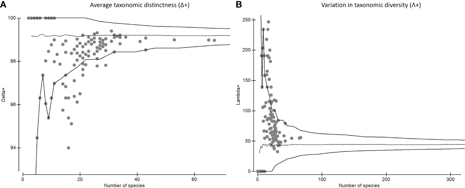
Figure 1 (A) Average taxonomic distinction index (Δ+) and (B) variation in taxonomic distinctness’ (Λ+) for the copepod community in the Eastern Pacific. The segmented line in red shows the mean, whereas the continuous lines are the distribution of probability at 95%.

Relationship of number of species, ES50 and environmental variables

The BRT+RAC model had the best fit to explain the number of species and retained six variables. The percentage of total deviance explained was approximately 85.2%. POC accounted for most of the relative influence (21.4%), followed by SSS, spatial autocovariate, SSS (range), SST (range), and MLD (Table 1). Because spatial autocorrelation was detected in the BRT model without autocovariates (Table 1), we chose the BRT+RAC model given its lack of spatial autocorrelation (Moran’s index = 0.004; p value = 0.485) (Table 1).

Table 1

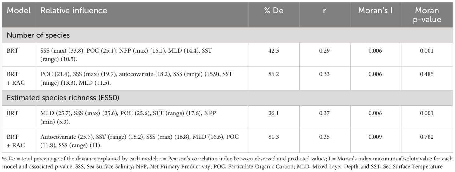
Table 1 Summary of the BRT Poisson and BRT + residual autocovariate (RAC) used to model number of species and estimated species richness (ES50) of copepods.

The BRT+RAC model had the best fit to explain the ES50 and retained six variables. The percentage of total deviance explained was approximately 81.3%. The autocovariate accounted for most of the relative influence (25.7%), followed by SST (range) (18.2%), SSS (max), MLD, POC, and SSS (range) (Table 1 and Supplementary Figure S3).

Observed and predicted latitudinal diversity gradients

The observed richness showed a heterogeneous pattern in the Eastern Pacific, with the highest values observed (291 species) off the coast of Alaska, Ecuador, northern Chile, and around 30°S–179°W (Figure 2A). ES50 showed a spatial pattern similar to that of the number of species, revealing the greatest richness at intermediate latitudes, with higher diversity in coastal areas in the Northern Hemisphere and in oceanic areas in the Southern Hemisphere (Figure 2B). The relationship of species richness and ES50 with latitude was significantly different from a unimodal distribution, indicating bimodality in both trends (Hartigan’s dip test, D = 0.048 and and D = 0.045; p-value < 0.01 and < 0.05, Figures 3A, B, respectively). Well-sampled cells were observed primarily at the Bering Sea, Gulf of Alaska, Gulf of Mexico, Eastern Tropical Pacific Ocean (ETPO), and the southern hemisphere between 40–58°S and 180°W (Supplementary Figures S4 and S5). The variogram model that best fit the pattern of species richness among the well-sampled cells was the Spherical function (sill = 1489; range = 588; nugget = 62; kappa = 1.7; Supplementary Table S3). The diversity predicted by R-K revealed higher predicted richness, with a maximum of 362 species (Figure 2C). The highest species richness was concentrated in continental margins, mainly in tropical and subtropical areas, and decreased in temperate areas. The difference between the observed and estimated richness showed extensive poorly sampled regions (Supplementary Figure S6), and higher residual variation was detected in the areas of low observed richness (Figure 2D). The species richness estimated by R-K showed a bimodal pattern (Hartigan’s dip test, D = 0.059; p-value < 0.05) (see Supplementary Figure S7).

Figure 2

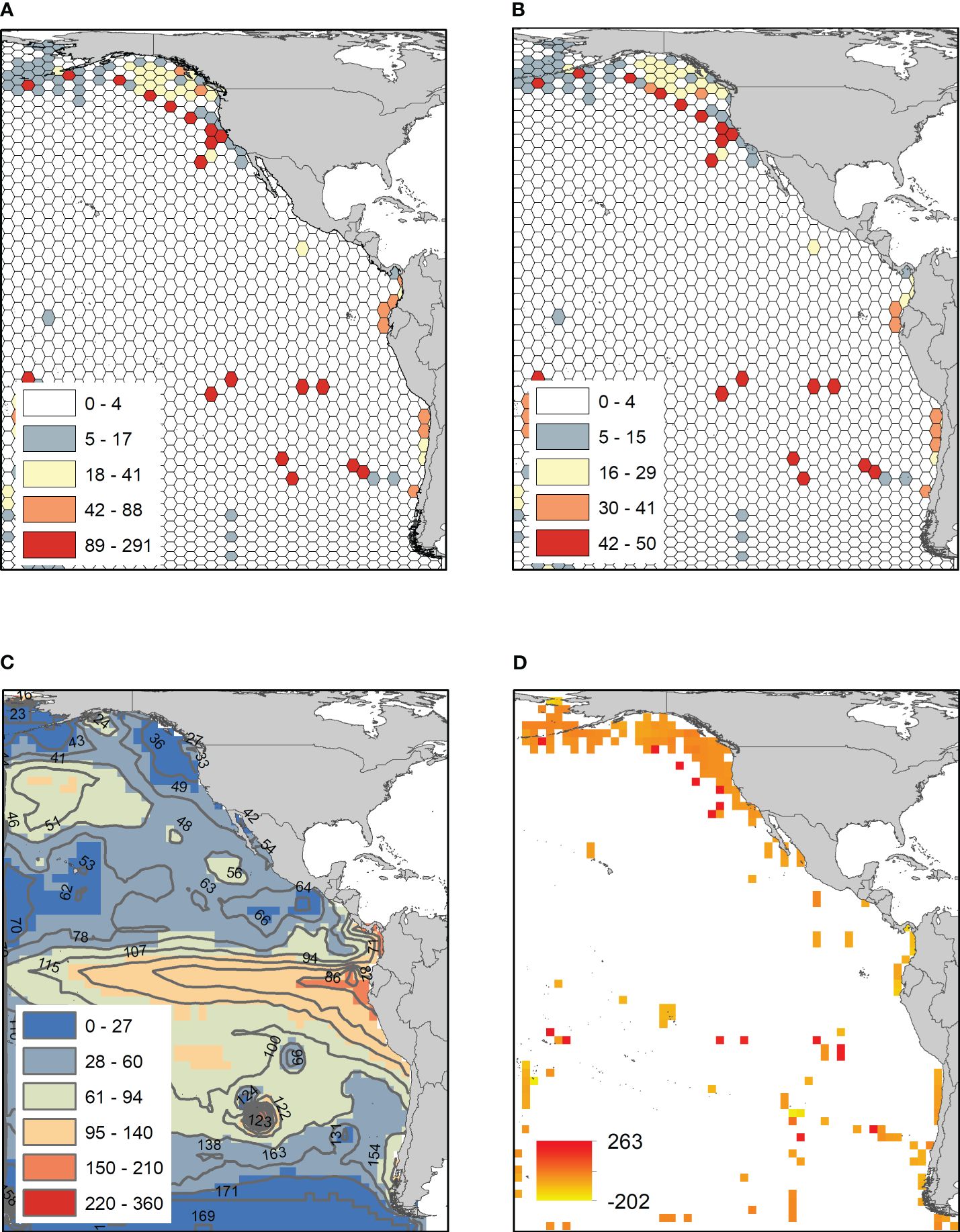
Figure 2 (A) Spatial distribution of number of species, (B) estimated species richness (ES50), (C) richness estimated from Regression-Kriging, and (D) residuals. Isolines represent richness predicted by R-K. Datum=WGS84. The map was constructed with ArcGIS 10.4.1 (ESRI, 2016). Map uses Behrmann equal area projection.

Figure 3

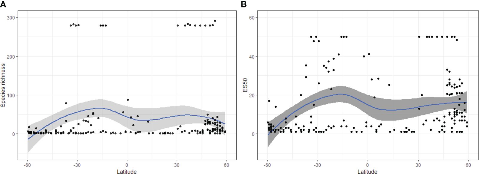
Figure 3 (A) Bimodality of number of species and (B) estimated species richness (ES50) of Eastern Pacific copepods. Black dots = empirical species richness; blue line = estimated trend; gray shade represents 95% point wise confidence interval. The figure was constructed with R software (R Core Team, 2023).

Spatial patterns of beta diversity

GDM explained 53.8% of the deviance in beta diversity. The predictors with the best fit to explain this pattern were geographical distance, SST (range), POC, SSS (max), NPP (min), MLD, and SST (range) (Supplementary Figure S8). Spatial prediction of the variation in copepod composition revealed regions with similar copepod communities distributed along a latitudinal gradient (Figure 4A). The composition differs between the temperate and equatorial zones, as well as between oceanic and continental areas (Figure 4A). Cluster analysis revealed four areas with similar species composition. The areas were numbered latitudinally from C1 to C4 for better interpretation (see Figure 4B). There is an exclusive group for the Northern Hemisphere in temperate and cold zones (C1) covering the Bering Sea, Gulf of Alaska, and part of the California Current, and another exclusive group for the Southern Hemisphere (C4) in the Southern Ocean (Figure 4B). The C2 cluster is shared between both hemispheres and is mainly oceanic, whereas the C3 cluster is oceanic-coastal with a large latitudinal distribution, encompassing the Humboldt Current System and the Pacific Central-American coast (Figure 4B).

Figure 4

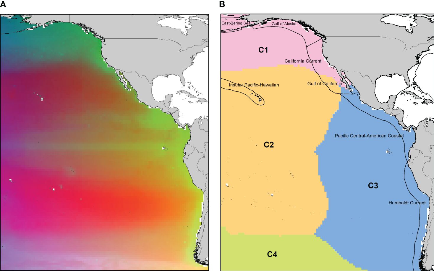
Figure 4 (A) Predicted spatial variation in copepods species composition. Locations with similar colors are expected to contain similar communities. (B) Map illustrating the clustering of GDM. A four-class classification of the region derived from predicted dissimilarities (C1 to C4). Symbol colors represent each plot’s membership in a specific assemblage. The figure was constructed with ArcGIS 10.4.1 (ESRI, 2016). Map uses Behrmann equal area projection.

Discussion

The geographic tendency of the specific richness of copepods in the Eastern Pacific is concordant with the bimodal pattern previously described for other taxa (e.g., Chaudhary et al., 2016; Saeedi et al., 2017; Rivadeneira and Poore, 2020; Pamungkas and Glasby, 2021), showing a significant asymmetric and bimodal pattern with higher diversity in the Northern Hemisphere (Figures 2A, B, and Supplementary Figure S7). From an ecological perspective, the bimodal pattern reported for copepods has the potential to be explained by SST, bathymetry, and NPP. Regarding temperature, this could exclude species intolerant to high values that are typical in tropical areas (Chaudhary and Costello, 2023). Regarding bathymetry, a wider continental margin in the Northern Hemisphere would provide a larger habitat, which is concordant with the species-area hypothesis (Lomolino, 2000). This is complemented by high primary productivity, which is characteristic of upwelling zones in the North Pacific (Zaytsev et al., 2003) and in the South Pacific off the coast of Chile and Peru (Escribano et al., 2012). Other mechanisms that have not been explicitly evaluated to date, such as physiological limitations, biotic interactions, and trophic resource availability, could also explain the dip in species richness in the equatorial zones (Chaudhary et al., 2016; Chaudhary and Costello, 2023). Therefore, the bimodality and asymmetry of species richness indicate that there is not only a general factor that determines diversity patterns on a broad scale. These tendencies could be investigated in regional studies to evaluate the effect of biotic interactions (e.g., co-occurrence) as a potential causal mechanism for bimodality.

According to the BRT+RAC model, the most important variables that explained and modulated the number of species were POC, SSS (max), and autocovariate (Table 1). Although there is no single predictor of species richness, there are fundamental variables, such as temperature, that modulate the large-scale patterns of pelagic diversity (Rombouts et al., 2009; Tittensor et al., 2010). Based on to Tittensor et al. (2010), SST alone is one of the most efficient predictors of coastal and oceanic species distribution on a global scale. Our results revealed that variability of temperature, and not its average value, was an efficient predictor of richness along the latitudinal gradient. Therefore, high temperature variability, together with the presence of warm waters in the equator, could constitute the main cause of the observed bimodal gradient because equatorial regions are too warm for some species (Chaudhary et al., 2021). Another physical mechanism that could explain the difference between areas of high diversity in the subtropics and less diversity in the equatorial zone would be the presence of two opposing currents (Equatorial Counter Current and South Equatorial Current). These two currents have distinct hydrological features: the warm pool to the west and the Pacific Equatorial Divergence, regions separated by well-defined fronts in salinity, pC02, and macronutrients (Le Borgne et al., 2002). These physical characteristics would generate a barrier such as the East Pacific Barrier reported for tropical fish (Gaither et al., 2016), and plankton (Bowen et al., 2016), which would limit the spread of organisms with a consequent break in diversity.

Regarding SSS as a modulator of species richness, it has a direct influence on feeding and egg production (Dutz and Christensen, 2018), growth rate, and population composition (Magouz et al., 2021), which are factors that ecologically regulate the community structure of the systems. Another modulator of copepod diversity is NPP, which has a positive relationship with richness, and a reported trend for marine and terrestrial organisms (Mittelbach et al., 2001; Chase and Leibold, 2002; Woodd-Walker et al., 2002; Fukami and Morin, 2003; Rombouts et al., 2009). This relationship can be explained by the fact that productivity is a key factor in the composition of copepod diets (Vargas et al., 2006, 2010). This is particularly important in coastal upwelling systems, given that high-quality food resources and lower temperature variability exert an advantageous effect on copepods, despite constituting an advective environment that may generate important changes in their life cycles (Peterson, 1998), biomass, and abundance (Escribano et al., 2012; Medellín-Mora et al., 2016) with potential consequences for the ecosystem food web.

Another important factor spatially structuring the observed and estimated diversity of copepods is the MLD, which indicates the relevant (effective) temperature of the upper-ocean copepods at a macroscale (Rombouts et al., 2009, 2011; Rajakaruna and Lewis, 2018). Indeed, a strong negative relationship was observed between diversity and MLD (Supplementary Figure S3) indicating that diversity was high in stratified waters, which may be due to that a stable physical structure in the near-surface ocean provides higher vertical niche availability than can support a high number of species (Rutherford et al., 1999). Indeed, copepod diversity was higher in areas with stable seasonal ocean temperatures, trends that have also been reported for the Atlantic Ocean (Woodd-Walker et al., 2002). This result corresponds with the observation that oligotrophic regions, with low seasonal variability have high copepod diversity (Medellín-Mora et al., 2021).

The high contribution of POC to the spatial variability of copepod richness is related to the fact that zooplankton in general, are important mediators of the flux of organic material into the deep ocean through contributions to both the active and passive carbon fluxes (the biological pump) (Ducklow et al., 2001), and their community composition has a significant influence on particle export, repackaging of POC with depth, carbon attenuation, and export through the mesopelagic zone (Steinberg et al., 2008; Wilson et al., 2008). In this regard, Omand et al. (2015) pointed out that disaggregation of large POC by zooplankton and the detrainment of POC-rich water from the mixed layer via the so-called mixed-layer pump (Gardner et al., 1995) constitutes one of the mechanisms that explain the export of small particles (0.2 to 20 μm) to depths up to 1000 m (Dall’Olmo and Mork, 2014). The discrepancies in POC, SST and SSS values in the Pacific Ocean are influenced by a complex interaction of various factors (Gebbie and Huybers, 2012). These factors include different water masses present in the region and the circulation patterns of the thermohaline current (Gebbie and Huybers, 2012). These water masses originate from different geographical areas and exhibit a variety of temperatures, salinity levels and ages, which interact and intermingle. The thermohaline current plays a fundamental role in this process, as it facilitates the transport of warm and saline waters towards higher latitudes, while directing cold and less saline waters towards lower latitudes. This causes significant mixing in the subtropical and tropical regions of the ocean, and therefore could constitute a macroscale structuring of the unequal distribution of species richness along the latitudinal gradient (Emery, 2001).

Our species richness prediction allowed us to identify areas of high diversity on the coasts of the Gulf of Alaska, California Current, Eastern Tropical Pacific Ocean (ETPO), and central-northern Chile (Figure 2B). The reported pattern can represent the differential sampling effort made in both hemispheres, with gaps and biases in the spatial distribution of the occurrences (Hickisch et al., 2019; Maitner et al., 2023). To overcome these limitations, the R-K method based on well-sampled cells (see Supplementary Figure S4) was used to fill these gaps (Lobo et al., 2018). Robustness in the prediction of the variation on richness by R-K at a broad geographic scale is supported by considering the autocorrelation intrinsically present in species richness (Legendre, 1993; Dormann, 2007; Snickars et al., 2014; Alves et al., 2020), allowing for a better understanding of the drivers of its geographic variation (Diniz et al., 2003; Dormann, 2007). Similarly, the latitudinal gradient of beta diversity showed changes from the coastal to the open ocean, as well as between hemispheres (see Figure 4A). For the East Pacific, the four clusters (Figure 4B) represent unique communities, suggesting high idiosyncratic and dispersal limitations in the East Pacific. The spatial tendency of the composition revealed an area exclusive to the Northern Hemisphere and one in the Southern Hemisphere, and two shared clusters in the temperate and southern regions (Figure 4B). This indicates that although there is a bimodal gradient of richness, the specific composition has a defined structure that obeys the dynamics of the current systems in both hemispheres (e.g., California Current, Humboldt Current System, Pacific Equatorial Countercurrent and North/South Pacific Subtropical Gyres) with a unique fauna with high levels of endemism as a result of basin-scale circulation patterns and mesoscale eddies, which come from the coastal upwelling zone, generating plankton transport (Medellín-Mora et al., 2021).

GDM revealed that the turnover in community composition changed at a greater rate with increasing geographical distance, SSS (range), and POC, showing a broad latitudinal gradient in turnover from Alaska to Tierra del Fuego (Figure 4A). The relationship was approximately linear for SST (range), indicating a weak effect on compositional turnover along these gradients (Supplementary Figure S9), for which processes related to oceanographic dynamics, such as POC circulation, productivity, and MLD, were the main modulators of replacement patterns. The productivity gradients are strongly influenced by local winds, bathymetry, and upwelling patterns (Sobarzo et al., 2007; Medellín-Mora et al., 2021), which generates heterogeneity in the water column chemistry. These environmental gradients can generate shifts in species composition and diversity patterns, as has been reported in some groups, such as phytoplankton on a global scale (Righetti et al., 2019), as well as in other regions, such as the South Australian Gulfs and semi-enclosed bays in Victoria (Leaper et al., 2011). An aspect of interest in future research would be to evaluate the patterns of community composition in upwelling and non-upwelling regions to study regional processes that may affect species turnover at the mesoscale.

To our knowledge, quantitative analysis and prediction of beta diversity have not yet been conducted in copepods of the East Pacific (but see Chaudhary and Costello, 2023 for a different approach). Knowledge of these geographic trends contributes to a better understanding of species shifts and similarities across broad environmental gradients (Buckley and Jetz, 2008; Jankowski et al., 2009). The geographic patterns of the composition of copepods studied through GDM constitute the first explicit analysis of a large dataset to geographically delimit regions confirmed by changes in copepod communities.

A critical aspect in the study of spatial patterns of diversity is the limitation that may be generated by spatial and temporal biases in the occurrence of species (Boakes et al., 2010; Bowler et al., 2022). The availability of occurrences on a global scale through OBIS is valuable for the study of marine macroecological patterns; that together with an appropriate curation and utilization of suitable statistical tools that consider autocorrelation (e.g., spatial regression, geostatistics) allows the identification of diversity trends on a broad geographic scale (see Alves et al., 2020; Cavalcante et al., 2022). Indeed, spatial prediction techniques, such as R-K and GDM, allow the generation of a robust prediction in regions that are less studied, enabling the overcoming of shortfalls in knowledge that limit our understanding of diversity patterns and gradients (see Hortal and Lobo, 2011; Alves et al., 2020).

Finally, knowledge on the main ecological factors driving diversity patterns (richness and composition) of copepods constitutes an important opportunity for understanding ecological processes that operate on a broad geographic scale and allows the identification of areas where greater sampling efforts are required.

Data availability statement

The original contributions presented in the study are included in the article/Supplementary Material. Further inquiries can be directed to the corresponding author.

Author contributions

RR: Conceptualization, Data curation, Formal analysis, Methodology, Writing – original draft, Writing – review & editing. RE: Conceptualization, Writing – original draft, Writing – review & editing. CG: Formal analysis, Writing – review & editing. MP-A: Conceptualization, Formal analysis, Writing – review & editing.

Funding

The author(s) declare financial support was received for the research, authorship, and/or publication of this article. This work was funded by Grant the Millennium Institute of Oceanography (Grant ICN12_019N.

Acknowledgments

RR thanks Magdalena Sanhueza for her constructive and critical comments on the manuscript.

Conflict of interest

The authors declare that the research was conducted in the absence of any commercial or financial relationships that could be construed as a potential conflict of interest.

Publisher’s note

All claims expressed in this article are solely those of the authors and do not necessarily represent those of their affiliated organizations, or those of the publisher, the editors and the reviewers. Any product that may be evaluated in this article, or claim that may be made by its manufacturer, is not guaranteed or endorsed by the publisher.

Supplementary material

The Supplementary Material for this article can be found online at: https://www.frontiersin.org/articles/10.3389/fevo.2024.1305916/full#supplementary-material.

References

Alves D. M. C. C., Eduardo A. A., da Silva Oliveira E. V., Villalobos F., Dobrovolski R., Pereira T. C., et al. (2020). Unveiling geographical gradients of species richness from scant occurrence data. Glob. Ecol. Biogeogr. 29, 748–759. doi: 10.1111/geb.13055

CrossRef Full Text | Google Scholar

Assis J., Tyberghein L., Bosch S., Verbruggen H., Serrão E. A., De Clerck O. (2018). Bio-ORACLE v2.0: Extending marine data layers for bioclimatic modelling. Glob. Ecol. Biogeogr. 27, 277–284. doi: 10.1111/geb.12693

CrossRef Full Text | Google Scholar

Ball-Damerow J. E., Brenskelle L., Barve N., Soltis P. S., Sierwald P., Bieler R., et al. (2019). Research applications of primary biodiversity databases in the digital age. PloS One 14, 1–26. doi: 10.1371/journal.pone.0215794

CrossRef Full Text | Google Scholar

Barton A. D., Dutkiewicz S., Flierl G., Bragg J., Follows M. J. (2010). Patterns of diversity in marine phytoplankton. Sci. (80-.). 327, 1509–1511. doi: 10.1126/science.1184961

CrossRef Full Text | Google Scholar

Baselga A. (2010). Partitioning the turnover and nestedness components of beta diversity. Glob. Ecol. Biogeogr. 19, 134–143. doi: 10.1111/j.1466-8238.2009.00490.x

CrossRef Full Text | Google Scholar

Beaugrand G., Rombouts I., Kirby R. R. (2013). Towards an understanding of the pattern of biodiversity in the oceans. Glob. Ecol. Biogeogr. 22, 440–449. doi: 10.1111/geb.12009

CrossRef Full Text | Google Scholar

Beck J., Böller M., Erhardt A., Schwanghart W. (2014). Spatial bias in the GBIF database and its effect on modeling species’ geographic distributions. Ecol. Inform. 19, 10–15. doi: 10.1016/j.ecoinf.2013.11.002

CrossRef Full Text | Google Scholar

Bivand R. (2022). spdep: spatial dependence: weighting schemes, statistics. Available at: https://github.com/r-spatial/spdep/.

Google Scholar

Boakes E. H., McGowan P. J. K., Fuller R. A., Chang-qing D., Clark N. E., O’Connor K., et al. (2010). Distorted views of biodiversity: spatial and temporal bias in species occurrence data. PloS Biol. 8, e1000385. doi: 10.1371/journal.pbio.1000385

PubMed Abstract | CrossRef Full Text | Google Scholar

Bowen B. W., Gaither M. R., DiBattista J. D., Iacchei M., Andrews K. R., Grant W. S., et al. (2016). Comparative phylogeography of the ocean planet. Proc. Natl. Acad. Sci. 113, 7962–7969. doi: 10.1073/pnas.1602404113

CrossRef Full Text | Google Scholar

Bowler D. E., Callaghan C. T., Bhandari N., Henle K., Benjamin Barth M., Koppitz C., et al. (2022). Temporal trends in the spatial bias of species occurrence records. Ecography (Cop.). 2022, 1–13. doi: 10.1111/ecog.06219

CrossRef Full Text | Google Scholar

Boyd R. J., Powney G. D., Carvell C., Pescott O. L. (2021). occAssess: An R package for assessing potential biases in species occurrence data. Ecol. Evol. 11, 16177–16187. doi: 10.1002/ece3.8299

PubMed Abstract | CrossRef Full Text | Google Scholar

Brandão M. C., Benedetti F., Martini S., Soviadan Y. D., Irisson J. O., Romagnan J. B., et al. (2021). Macroscale patterns of oceanic zooplankton composition and size structure. Sci. Rep. 11, 1–19. doi: 10.1038/s41598-021-94615-5

PubMed Abstract | CrossRef Full Text | Google Scholar

Brayard A., Escarguel G., Bucher H. (2005). Latitudinal gradient of taxonomic richness: combined outcome of temperature and geographic mid-domains effects? J. Zool. Syst. Evol. Res. 43, 178–188. doi: 10.1111/j.1439-0469.2005.00311.x

CrossRef Full Text | Google Scholar

Brown J. L., Cameron A., Yoder A. D., Vences M. (2014). A necessarily complex model to explain the biogeography of the amphibians and reptiles of Madagascar. Nat. Commun. 5, 5046. doi: 10.1038/ncomms6046

PubMed Abstract | CrossRef Full Text | Google Scholar

Buckley L. B., Jetz W. (2008). Linking global turnover of species and environments. Proc. Natl. Acad. Sci. U. S. A. 105, 17836–17841. doi: 10.1073/pnas.0803524105

PubMed Abstract | CrossRef Full Text | Google Scholar

Burnham K., Anderson D. (2004). Model selection and multimodel inference. A Practical Information-Theoretic Approach (New York: Springer), 2nd ed. 488p

Google Scholar

Cavalcante T., Weber M. M., Barnett A. A. (2022). Combining geospatial abundance and ecological niche models to identify high-priority areas for conservation: The neglected role of broadscale interspecific competition. Front. Ecol. Evol. 10. doi: 10.3389/fevo.2022.915325

CrossRef Full Text | Google Scholar

Chase J., Leibold M. (2002). Chase JM, Leibold MA. Spatial scale dictates the productivity-biodiversity relationship. Nature 416: 427-430. Nature 416, 427–430. doi: 10.1038/416427a

PubMed Abstract | CrossRef Full Text | Google Scholar

Chaudhary C., Costello M. J. (2023). Marine species turnover but not richness, peaks at the Equator. Prog. Oceanogr. 210, 102941. doi: 10.1016/j.pocean.2022.102941

CrossRef Full Text | Google Scholar

Chaudhary C., Richardson A. J., Schoeman D. S., Costello M. J. (2021). Global warming is causing a more pronounced dip in marine species richness around the equator. Proc. Natl. Acad. Sci. 118, e2015094118. doi: 10.1073/pnas.2015094118

CrossRef Full Text | Google Scholar

Chaudhary C., Saeedi H., Costello M. J. (2016). Bimodality of latitudinal gradients in marine species richness. Trends Ecol. Evol. 31, 670–676. doi: 10.1016/j.tree.2016.06.001

PubMed Abstract | CrossRef Full Text | Google Scholar

Chaudhary C., Saeedi H., Costello M. J. (2017). Marine species richness is bimodal with latitude: A reply to fernandez and marques. Trends Ecol. Evol. 32, 234–237. doi: 10.1016/j.tree.2017.02.007

PubMed Abstract | CrossRef Full Text | Google Scholar

Clarke K., Gorley R. (2015). PRIMER version 7: User manual/tutorial. PRIMER-E: Plymouth, 192..

Google Scholar

Clarke K. R., Warwick R. M. (1998). A taxonomic distinctness index and its statistical properties. J. Appl. Ecol. 35, 523–531. doi: 10.1046/j.1365-2664.1998.3540523.x

CrossRef Full Text | Google Scholar

Crase B., Liedloff A. C., Wintle B. A. (2012). A new method for dealing with residual spatial autocorrelation in species distribution models. Ecography (Cop.). 35, 879–888. doi: 10.1111/j.1600-0587.2011.07138.x

CrossRef Full Text | Google Scholar

Currie D. J. (1991). Energy and large-scale patterns of animal- and plant-species richness. Am. Nat. 137, 27–49. doi: 10.1086/285144

CrossRef Full Text | Google Scholar

D’Antraccoli M., Bedini G., Peruzzi L. (2022). Maps of relative floristic ignorance and virtual floristic lists: An R package to incorporate uncertainty in mapping and analysing biodiversity data. Ecol. Inform. 67, 101512. doi: 10.1016/j.ecoinf.2021.101512

CrossRef Full Text | Google Scholar

Dall’Olmo G., Mork K. A. (2014). Carbon export by small particles in the Norwegian Sea. Geophys. Res. Lett. 41, 2921–2927. doi: 10.1002/2014GL059244

CrossRef Full Text | Google Scholar

Diniz J., Bini L. M., Hawkins B. A., Alexandre J., Diniz-Filho F., Bini L. M. (2003). Spatial autocorrelation and red herrings in geographical ecology. Glob. Ecol. Biogeogr. 12, 53–64. doi: 10.1046/j.1466-822X.2003.00322.x

CrossRef Full Text | Google Scholar

Dormann C. F. (2007). Effects of incorporating spatial autocorrelation into the analysis of species distribution data. Glob. Ecol. Biogeogr. 16, 129–138. doi: 10.1111/j.1466-8238.2006.00279.x

CrossRef Full Text | Google Scholar

Dormann C. F., Elith J., Bacher S., Buchmann C., Carl G., Carré G., et al. (2013). Collinearity: A review of methods to deal with it and a simulation study evaluating their performance. Ecography (Cop.). 36, 27–46. doi: 10.1111/j.1600-0587.2012.07348.x

CrossRef Full Text | Google Scholar

Dornelas M., Antão L. H., Moyes F., Bates A. E., Magurran A. E., Adam D., et al. (2018). BioTIME: A database of biodiversity time series for the Anthropocene. Glob. Ecol. Biogeogr. 27, 760–786. doi: 10.1111/geb.12729

PubMed Abstract | CrossRef Full Text | Google Scholar

Ducklow H. W., Steinberg D. K., William C., Point M. G., Buesseler K. O. (2001). Upper ocean carbon export and the biological pump. Oceanography 14, 50–58. doi: 10.5670/oceanog

CrossRef Full Text | Google Scholar

Dutz J., Christensen A. M. (2018). Broad plasticity in the salinity tolerance of a marine copepod species, Acartia longiremis, in the Baltic Sea. J. Plankton Res. 40, 342–355. doi: 10.1093/plankt/fby013

CrossRef Full Text | Google Scholar

Elith J., Leathwick J. R., Hastie T. (2008). A working guide to boosted regression trees. J. Anim. Ecol. 77, 802–813. doi: 10.1111/j.1365-2656.2008.01390.x

PubMed Abstract | CrossRef Full Text | Google Scholar

Emery W. (2001). Water types and water masses. Encycl. Ocean Sci. 4, 3179–3187. doi: 10.1006/rwos.2001.0108

CrossRef Full Text | Google Scholar

Escalle L., Pennino M. G., Gaertner D., Chavance P., Delgado de Molina A., Demarcq H., et al. (2016). Environmental factors and megafauna spatio-temporal co-occurrence with purse-seine fisheries. Fish. Oceanogr. 25, 433–447. doi: 10.1111/fog.12163

CrossRef Full Text | Google Scholar

Escribano R., Hidalgo P. (2000). Spatial distribution of copepods in the north of the Humboldt Current region off Chile during coastal upwelling. J. Mar. Biol. Assoc. United Kingdom 80, 283–290. doi: 10.1017/S002531549900185X

CrossRef Full Text | Google Scholar

Escribano R., Hidalgo P., Fuentes M., Donoso K. (2012). Zooplankton time series in the coastal zone off Chile: Variation in upwelling and responses of the copepod community. Prog. Oceanogr. 97–100, 174–186. doi: 10.1016/j.pocean.2011.11.006

CrossRef Full Text | Google Scholar

ESRI. (2016). ArcGIS desktop (Redlands, CA: Envrionmental Systems Research Institute). Release 10.4.1.

Google Scholar

Fautin D. G., Malarky L., Soberón J. (2013). Latitudinal diversity of sea anemones (cnidaria: Actiniaria). Biol. Bull. 224, 89–98. doi: 10.1086/BBLv224n2p89

PubMed Abstract | CrossRef Full Text | Google Scholar

Fernandez M. O., Marques A. C. (2017). Diversity of diversities: A response to chaudhary, saeedi, and costello. Trends Ecol. Evol. 32, 232–234. doi: 10.1016/j.tree.2016.10.013

PubMed Abstract | CrossRef Full Text | Google Scholar

Ferrier S., Manion G., Elith J., Richardson K. (2007). Using generalized dissimilarity modelling to analyse and predict patterns of beta diversity in regional biodiversity assessment. Divers. Distrib. 13, 252–264. doi: 10.1111/j.1472-4642.2007.00341.x

CrossRef Full Text | Google Scholar

Fitzpatrick M. C., Mokany K., Manion G., Lisk M., Ferrier S., Nieto-Lugilde D. (2020). gdm: generalized dissimilarity modeling. Available at: https://cran.r-project.org/package=gdm.

Google Scholar

Fitzpatrick M. C., Sanders N. J., Normand S., Svenning J.-C., Ferrier S., Gove A. D., et al. (2013). Environmental and historical imprints on beta diversity: insights from variation in rates of species turnover along gradients. Proc. Biol. Sci. 280, 20131201. doi: 10.1098/rspb.2013.1201

PubMed Abstract | CrossRef Full Text | Google Scholar

Fragkopoulou E., Serrão E. A., De Clerck O., Costello M. J., Araújo M. B., Duarte C. M., et al. (2022). Global biodiversity patterns of marine forests of brown macroalgae. Glob. Ecol. Biogeogr. 31, 636–648. doi: 10.1111/geb.13450

CrossRef Full Text | Google Scholar

Fukami T., Morin P. J. (2003). Productivity-biodiversity relationships depend on the history of community assembly. Nature 424, 423–426. doi: 10.1038/nature01785

PubMed Abstract | CrossRef Full Text | Google Scholar

Gagné T. O., Reygondeau G., Jenkins C. N., Sexton J. O., Bograd S. J., Hazen E. L., et al. (2020). Towards a global understanding of the drivers of marine and terrestrial biodiversity. PloS One 15, e0228065. doi: 10.1371/journal.pone.0228065

PubMed Abstract | CrossRef Full Text | Google Scholar

Gaither M. R., Bowen B. W., Rocha L. A., Briggs J. C. (2016). Fishes that rule the world: circumtropical distributions revisited. Fish Fish. 17, 664–679. doi: 10.1111/faf.12136

CrossRef Full Text | Google Scholar

Gardner W. D., Chung S. P., Richardson M. J., Walsh I. D. (1995). The oceanic mixed-layer pump. Deep Sea Res. Part II Top. Stud. Oceanogr. 42, 757–775. doi: 10.1016/0967-0645(95)00037-Q

CrossRef Full Text | Google Scholar

Gebbie G., Huybers P. (2012). The mean age of ocean waters inferred from radiocarbon observations: Sensitivity to surface sources and accounting for mixing histories. J. Phys. Oceanogr. 42, 291–305. doi: 10.1175/JPO-D-11-043.1

CrossRef Full Text | Google Scholar

González C. E., Medellín-Mora J., Escribano R. (2020). Environmental gradients and spatial patterns of calanoid copepods in the southeast pacific. Front. Ecol. Evol. 8. doi: 10.3389/fevo.2020.554409

CrossRef Full Text | Google Scholar

Gotelli N., Colwell R. (2011). “Estimating species richness,” in Frontiers in measuring biodiversity (United Kingdom: Oxford University Press), 39–54.

Google Scholar

Greenwell B., Boehmke B., Cunningham J., Developers G. B. M. (2022). gbm: generalized boosted regression models. Available at: https://cran.r-project.org/package=gbm.

Google Scholar

Guillaumot C., Moreau C., Danis B., Saucède T. (2020). Extrapolation in species distribution modelling. Application to Southern Ocean marine species. Prog. Oceanogr. 188, 102438. doi: 10.1016/j.pocean.2020.102438

CrossRef Full Text | Google Scholar

Hartigan J. A., Hartigan P. M. (1985). The dip test of unimodality. Ann. Stat. 13, 70–84. doi: 10.1214/aos/1176346577

CrossRef Full Text | Google Scholar

Hawkins B. A., Field R., Cornell H. V., Currie D. J., Guégan J.-F., Kaufman D. M., et al. (2003). Energy, water, and broad-scale geographic patterns of species richness. Ecology 84, 3105–3117. doi: 10.1890/03-8006

CrossRef Full Text | Google Scholar

Hays G. C., Richardson A. J., Robinson C. (2005). Climate change and marine plankton. Trends Ecol. Evol. 20, 337–344. doi: 10.1016/j.tree.2005.03.004

PubMed Abstract | CrossRef Full Text | Google Scholar

Hickisch R., Hodgetts T., Johnson P. J., Sillero-Zubiri C., Tockner K., Macdonald D. W. (2019). Effects of publication bias on conservation planning. Conserv. Biol. 33, 1151–1163. doi: 10.1111/cobi.13326

PubMed Abstract | CrossRef Full Text | Google Scholar

Hiemstra P. H., Pebesma E. J., Twenhöfel C. J. W., Heuvelink G. B. M. (2009). Real-time automatic interpolation of ambient gamma dose rates from the Dutch radioactivity monitoring network. Comput. Geosci. 35, 1711–1721. doi: 10.1016/j.cageo.2008.10.011

CrossRef Full Text | Google Scholar

Hijmans R. J. (2023). raster: geographic data analysis and modeling. Available at: https://rspatial.org/raster.

Google Scholar

Hijmans R. J., Phillips S., Leathwick J., Elith J. (2021). dismo: species distribution modeling. Available at: https://rspatial.org/raster/sdm/.

Google Scholar

Hooff R. C., Peterson W. T. (2006). Copepod biodiversity as an indicator of changes in ocean and climate conditions of the northern California current ecosystem. Limnol. Oceanogr. 51, 2607–2620. doi: 10.4319/lo.2006.51.6.2607

CrossRef Full Text | Google Scholar

Hortal J., Jiménez-Valverde A., Gómez J. F., Lobo J. M., Baselga A. (2008). Historical bias in biodiversity inventories affects the observed environmental niche of the species. Oikos 117, 847–858. doi: 10.1111/j.0030-1299.2008.16434.x

CrossRef Full Text | Google Scholar

Hortal J., Lobo J. M. (2011). Can species richness patterns be interpolated from a limited number of well-known areas? Mapping diversity using GLM and kriging. Nat. Conserv. 9, 200–207. doi: 10.4322/natcon.2011.026

CrossRef Full Text | Google Scholar

Hughes A. C., Orr M. C., Ma K., Costello M. J., Waller J., Provoost P., et al. (2021). Sampling biases shape our view of the natural world. Ecography (Cop.). 44, 1259–1269. doi: 10.1111/ecog.05926

CrossRef Full Text | Google Scholar

Irigoien X., Huisman J., Harris R. P. (2004). Global biodiversity patterns of marine phytoplankton and zooplankton. Nature 429, 863–867. doi: 10.1038/nature02593

PubMed Abstract | CrossRef Full Text | Google Scholar

Isaac N. J. B., Pocock M. J. O. (2015). Bias and information in biological records. Biol. J. Linn. Soc 115, 522–531. doi: 10.1111/bij.12532

CrossRef Full Text | Google Scholar

Jankowski J. E., Ciecka A. L., Meyer N. Y., Rabenold K. N. (2009). Beta diversity along environmental gradients: implications of habitat specialization in tropical montane landscapes. J. Anim. Ecol. 78, 315–327. doi: 10.1111/j.1365-2656.2008.01487.x

PubMed Abstract | CrossRef Full Text | Google Scholar

Kassambara A., Mundt F. (2020). factoextra: extract and visualize the results of multivariate data analyses. Available at: https://cran.r-project.org/package=factoextra.

Google Scholar

Kerr J. (2001). Global biodiversity patterns: From description to understanding. Trends Ecol. Evol. 16, 424–425. doi: 10.1016/S0169-5347(01)02226-1

CrossRef Full Text | Google Scholar

Klein E., Appeltans W., Provoost P., Saeedi H., Benson A., Bajona L., et al. (2019). OBIS infrastructure, lessons learned, and vision for the future. Front. Mar. Sci. 6. doi: 10.3389/fmars.2019.00588

CrossRef Full Text | Google Scholar

Kuhn M. (2008). Building predictive models in R using the caret package. J. Stat. Software 28, 1–26. doi: 10.18637/jss.v028.i05

CrossRef Full Text | Google Scholar

Leaper R., Hill N. A., Edgar G. J., Ellis N., Lawrence E., Pitcher C. R., et al. (2011). Predictions of beta diversity for reef macroalgae across southeastern Australia. Ecosphere 2, 1–18. doi: 10.1890/ES11-00089.1

CrossRef Full Text | Google Scholar

Le Borgne R., Barber R. T., Delcroix T., Inoue H. Y., Mackey D. J., Rodier M. (2002). Pacific warm pool and divergence: Temporal and zonal variations on the equator and their effects on the biological pump. Deep. Res. Part II Top. Stud. Oceanogr. 49, 2471–2512. doi: 10.1016/S0967-0645(02)00045-0

CrossRef Full Text | Google Scholar

Legendre P. (1993). Spatial autocorrelation: trouble or new paradigm? Ecology 74, 1659–1673. doi: 10.2307/1939924

CrossRef Full Text | Google Scholar

Leprieur F., Tedesco P. A., Hugueny B., Beauchard O., Dürr H. H., Brosse S., et al. (2011). Partitioning global patterns of freshwater fish beta diversity reveals contrasting signatures of past climate changes. Ecol. Lett. 14, 325–334. doi: 10.1111/ele.2011.14.issue-4

PubMed Abstract | CrossRef Full Text | Google Scholar

Lin H.-Y., Corkrey R., Kaschner K., Garilao C., Costello M. J. (2021). Latitudinal diversity gradients for five taxonomic levels of marine fish in depth zones. Ecol. Res. 36, 266–280. doi: 10.1111/1440-1703.12193

CrossRef Full Text | Google Scholar

Lobo J. M., Hortal J., Yela J. L., Millán A., Sánchez-Fernández D., García-Roselló E., et al. (2018). KnowBR: An application to map the geographical variation of survey effort and identify well-surveyed areas from biodiversity databases. Ecol. Indic. 91, 241–248. doi: 10.1016/j.ecolind.2018.03.077

CrossRef Full Text | Google Scholar

Lomolino M. V. (2000). Ecology’s most general, yet protean pattern: the species-area relationship. J. Biogeogr. 27, 17–26. doi: 10.1046/j.1365-2699.2000.00377.x

CrossRef Full Text | Google Scholar

Maechler M. (2021). diptest: hartigan’s dip test statistic for unimodality - corrected. Available at: https://github.com/mmaechler/diptest.

Google Scholar

Magouz F. I., Essa M. A., Matter M., Mansour A. T., Gaber A., Ashour M. (2021). Effect of different salinity levels on population dynamics and growth of the cyclopoid copepod Oithona nana. Diversity 13, 1–10. doi: 10.3390/d13050190

CrossRef Full Text | Google Scholar

Maitner B., Gallagher R., Svenning J. C., Tietje M., Wenk E. H., Eiserhardt W. L. (2023). A global assessment of the Raunkiaeran shortfall in plants: geographic biases in our knowledge of plant traits. New Phytol. 240 (4), 1345–1354. doi: 10.1111/nph.18999

PubMed Abstract | CrossRef Full Text | Google Scholar

McArthur M. A., Brooke B. P., Przeslawski R., Ryan D. A., Lucieer V. L., Nichol S., et al. (2010). On the use of abiotic surrogates to describe marine benthic biodiversity. Estuar. Coast. Shelf Sci. 88, 21–32. doi: 10.1016/j.ecss.2010.03.003

CrossRef Full Text | Google Scholar

Medellín-Mora J., Escribano R., Corredor-Acosta A., Hidalgo P., Schneider W. (2021). Uncovering the composition and diversity of pelagic copepods in the oligotrophic blue water of the south pacific subtropical gyre. Front. Mar. Sci. 8. doi: 10.3389/fmars.2021.625842

CrossRef Full Text | Google Scholar

Medellín-Mora J., Escribano R., Schneider W. (2016). Community response of zooplankton to oceanographic changes, (2002-2012) in the central/southern upwelling system of Chile. Prog. Oceanogr. 142, 17–29. doi: 10.1016/j.pocean.2016.01.005

CrossRef Full Text | Google Scholar

Melo-Merino S. M., Reyes-Bonilla H., Lira-Noriega A. (2020). Ecological niche models and species distribution models in marine environments: A literature review and spatial analysis of evidence. Ecol. Modell. 415. doi: 10.1016/j.ecolmodel.2019.108837

CrossRef Full Text | Google Scholar

Menegotto A., Rangel T. F. (2018). Mapping knowledge gaps in marine diversity reveals a latitudinal gradient of missing species richness. Nat. Commun. 9, 4713. doi: 10.1038/s41467-018-07217-7

PubMed Abstract | CrossRef Full Text | Google Scholar

Miller E. C., Hayashi K. T., Song D., Wiens J. J. (2018). Explaining the ocean’s richest biodiversity hotspot and global patterns of fish diversity. Proc. Biol. Sci. 285, 1888. doi: 10.1098/rspb.2018.1314

CrossRef Full Text | Google Scholar

Mittelbach G. G., Steiner C. F., Scheiner S. M., Gross K. L., Reynolds H. L., Waide R. B., et al. (2001). What is the observed relationship between species richness and productivity? Ecology 82, 2381. doi: 10.2307/2679922

CrossRef Full Text | Google Scholar

Monsarrat S., Boshoff A. F., Kerley G. I. H. (2019). Accessibility maps as a tool to predict sampling bias in historical biodiversity occurrence records. Ecography (Cop.). 42, 125–136. doi: 10.1111/ecog.03944

CrossRef Full Text | Google Scholar

Moreno R. A., Labra F. A., Cotoras D. D., Camus P. A., Gutiérrez D., Aguirre L., et al. (2021). Evolutionary drivers of the hump-shaped latitudinal gradient of benthic polychaete species richness along the Southeastern Pacific coast. PeerJ 9, e12010. doi: 10.7717/peerj.12010

PubMed Abstract | CrossRef Full Text | Google Scholar

Naimi B., Hamm N. A. S., Groen T. A., Skidmore A. K., Toxopeus A. G. (2014). Where is positional uncertainty a problem for species distribution modelling? Ecography (Cop.). 37, 191–203. doi: 10.1111/j.1600-0587.2013.00205.x

CrossRef Full Text | Google Scholar

O’Brien T. D. (2014). COPEPOD: the global plankton database. Available at: https://www.st.nmfs.noaa.gov/copepod/.

Google Scholar

O’Brien C. J., Vogt M., Gruber N. (2016). Global coccolithophore diversity: Drivers and future change. Prog. Oceanogr. 140, 27–42. doi: 10.1016/j.pocean.2015.10.003

CrossRef Full Text | Google Scholar

Oksanen J., Simpson G. L., Blanchet F. G., Kindt R., Legendre P., Minchin P. R., et al. (2022). vegan: community ecology package. Available at: https://cran.r-project.org/package=vegan.

Google Scholar

Omand M. M., D’Asaro E. A., Lee C. M., Perry M. J., Briggs N., Cetinić I., et al. (2015). Eddy-driven subduction exports particulate organic carbon from the spring bloom. Sci. (80-.). 348, 222–225. doi: 10.1126/science.1260062

CrossRef Full Text | Google Scholar

Pamungkas J., Glasby C. J. (2021). Biogeography of polychaete worms (Annelida) of the world. Mar. Ecol. Prog. Ser. 657, 147–159. doi: 10.3354/meps13531

CrossRef Full Text | Google Scholar

Pebesma E. J. (2004). Multivariable geostatistics in {S}: the gstat package. Comput. Geosci. 30, 683–691. doi: 10.1016/j.cageo.2004.03.012

CrossRef Full Text | Google Scholar

Pebesma E., Graeler B. (2021). gstat: spatial and spatio-temporal geostatistical modelling, prediction and simulation. Available at: https://github.com/r-spatial/gstat/.

Google Scholar

Peterson W. (1998). Life cycle strategies of copepods in coastal upwelling zones. J. Mar. Syst. 15, 313–326. doi: 10.1016/S0924-7963(97)00082-1

CrossRef Full Text | Google Scholar

Pianka E. R. (1966). Latitudinal gradients in species diversity: A review of concepts. Am. Nat. 100, 33–46. doi: 10.1086/282398

CrossRef Full Text | Google Scholar

Provoost P., Bosch S. (2022). robis: ocean biodiversity information system (OBIS) client. Available at: https://github.com/iobis/robis.

Google Scholar

Rajakaruna H., Lewis M. (2018). Do yearly temperature cycles reduce species richness? Insights from calanoid copepods. Theor. Ecol. 11, 39–53. doi: 10.1007/s12080-017-0347-y

CrossRef Full Text | Google Scholar

Razouls C., Desreumaux N., Kouwenberg J., de Bovée F. (2023). Biodiversity of Marine Planktonic Copepods (morphology, geographical distribution and biological data) (Sorbonne University, CNRS). Available at: http://copepodes.obs-banyuls.fr/en (Accessed March 10, 2023]).

Google Scholar

R Core Team. (2023). R: A language and environment for statistical computing. Available at: https://www.r-project.org/.

Google Scholar

Righetti D., Vogt M., Gruber N., Psomas A., Zimmermann N. E. (2019). Global pattern of phytoplankton diversity driven by temperature and environmental variability. Sci. Adv. 5, 1–11. doi: 10.1126/sciadv.aau6253

CrossRef Full Text | Google Scholar

Rivadeneira M., Poore G. (2020). “Latitudinal Gradient of Diversity of Marine Crustaceans: TOWARDS a Synthesis”., 389–412. doi: 10.1093/oso/9780190637842.003.0015

CrossRef Full Text | Google Scholar

Rivera R., Escribano R., González C. E., Pérez-Aragón M. (2023). Modeling present and future distribution of plankton populations in a coastal upwelling zone: the copepod Calanus Chilensis as a study case. Sci. Rep. 13, 3158. doi: 10.1038/s41598-023-29541-9

PubMed Abstract | CrossRef Full Text | Google Scholar

Rocchini D., Hortal J., Lengyel S., Lobo J. M., Jiménez-Valverde A., Ricotta C., et al. (2011). Accounting for uncertainty when mapping species distributions: The need for maps of ignorance. Prog. Phys. Geogr. 35, 211–226. doi: 10.1177/0309133311399491

CrossRef Full Text | Google Scholar

Rohde K. (1992). Latitudinal gradients in species diversity: the search for the primary cause. Oikos 65, 514. doi: 10.2307/3545569

CrossRef Full Text | Google Scholar

Rombouts I., Beaugrand G., Ibaňez F., Chiba S., Legendre L. (2011). Marine copepod diversity patterns and the metabolic theory of ecology. Oecologia 166, 349–355. doi: 10.1007/s00442-010-1866-z

PubMed Abstract | CrossRef Full Text | Google Scholar

Rombouts I., Beaugrand G., Ibaňez F., Gasparini S., Chiba S., Legendre L. (2009). Global latitudinal variations in marine copepod diversity and environmental factors. Proc. R. Soc B Biol. Sci. 276, 3053–3062. doi: 10.1098/rspb.2009.0742

CrossRef Full Text | Google Scholar

Roy K., Jablonski D., Valentine J. W., Rosenberg G. (1998). Marine latitudinal diversity gradients: Tests of causal hypotheses. Proc. Natl. Acad. Sci. U. S. A. 95, 3699–3702. doi: 10.1073/pnas.95.7.3699

PubMed Abstract | CrossRef Full Text | Google Scholar

Ruete A. (2015). Displaying bias in sampling effort of data accessed from biodiversity databases using ignorance maps. Biodivers. Data J. 3, e5361. doi: 10.3897/BDJ.3.e5361

CrossRef Full Text | Google Scholar

Rutherford S., D’Hondt S., Prell W. (1999). Environmental controls on the geographic distribution of zooplankton diversity. Nature 400, 749–753. doi: 10.1038/23449

CrossRef Full Text | Google Scholar

Saeedi H., Costello M. J., Warren D., Brandt A. (2019a). Latitudinal and bathymetrical species richness patterns in the NW Pacific and adjacent Arctic Ocean. Sci. Rep. 9, 9303. doi: 10.1038/s41598-019-45813-9

PubMed Abstract | CrossRef Full Text | Google Scholar

Saeedi H., Dennis T. E., Costello M. J. (2017). Bimodal latitudinal species richness and high endemicity of razor clams (Mollusca). J. Biogeogr. 44, 592–604. doi: 10.1111/jbi.12903

CrossRef Full Text | Google Scholar

Saeedi H., Jacobsen N. L., Brandt A. (2022). Biodiversity and distribution of Isopoda and Polychaeta along the Northwestern Pacific and the Arctic Ocean. Biodivers. Inf. 17, 10–26. doi: 10.17161/bi.v17i.15581

CrossRef Full Text | Google Scholar

Saeedi H., Reimer J. D., Brandt M. I., Dumais P. O., Jażdżewska A. M., Jeffery N. W., et al. (2019b). Global marine biodiversity in the context of achieving the Aichi Targets: Ways forward and addressing data gaps. PeerJ 2019, 1–17. doi: 10.7717/peerj.7221

CrossRef Full Text | Google Scholar

Snickars M., Gullström M., Sundblad G., Bergström U., Downie A.-L., Lindegarth M., et al. (2014). Species–environment relationships and potential for distribution modelling in coastal waters. J. Sea Res. 85, 116–125. doi: 10.1016/j.seares.2013.04.008

CrossRef Full Text | Google Scholar

Sobarzo M., Bravo L., Donoso D., Garcés-Vargas J., Schneider W. (2007). Coastal upwelling and seasonal cycles that influence the water column over the continental shelf off central Chile. Prog. Oceanogr. 75, 363–382. doi: 10.1016/j.pocean.2007.08.022

CrossRef Full Text | Google Scholar

Steinberg D. K., Cope J. S., Wilson S. E., Kobari T. (2008). A comparison of mesopelagic mesozooplankton community structure in the subtropical and subarctic North Pacific Ocean. Deep Sea Res. Part II Top. Stud. Oceanogr. 55, 1615–1635. doi: 10.1016/j.dsr2.2008.04.025

CrossRef Full Text | Google Scholar

Stokes A. (2018). If not one, then all: Is incomplete support for any hypothesis support for all hypotheses? Prize. Writ. 138, 176–185. Available at: https://prizedwriting.ucdavis.edu/sites/prizedwriting.ucdavis.edu/files/sitewide/pastissues/17%E2%80%9318%20STOKES.pdf.

Google Scholar

Tessarolo G., Ladle R. J., Lobo J. M., Rangel T. F., Hortal J. (2021). Using maps of biogeographical ignorance to reveal the uncertainty in distributional data hidden in species distribution models. Ecography (Cop.). 44, 1743–1755. doi: 10.1111/ecog.05793

CrossRef Full Text | Google Scholar

Titley M. A., Snaddon J. L., Turner E. C. (2017). Scientific research on animal biodiversity is systematically biased towards vertebrates and temperate regions. PloS One 12, 1–14. doi: 10.1371/journal.pone.0189577

CrossRef Full Text | Google Scholar

Tittensor D. P., Mora C., Jetz W., Lotze H. K., Ricard D., Berghe E., et al. (2010). Global patterns and predictors of marine biodiversity across taxa. Nature 466, 1098–1101. doi: 10.1038/nature09329

PubMed Abstract | CrossRef Full Text | Google Scholar

Troudet J., Grandcolas P., Blin A., Vignes-Lebbe R., Legendre F. (2017). Taxonomic bias in biodiversity data and societal preferences. Sci. Rep. 7, 1–14. doi: 10.1038/s41598-017-09084-6

PubMed Abstract | CrossRef Full Text | Google Scholar

Vargas C. A., Escribano R., Poulet S. (2006). Phytoplankton food quality determines time windows for successful zooplankton reproductive pulses. Ecology 87, 2992–2999. doi: 10.1890/0012-9658(2006)87[2992:PFQDTW]2.0.CO;2

PubMed Abstract | CrossRef Full Text | Google Scholar

Vargas C. A., Martínez R. A., Escribano R., Lagos N. A. (2010). Seasonal relative influence of food quantity, quality, and feeding behaviour on zooplankton growth regulation in coastal food webs. J. Mar. Biol. Assoc. United Kingdom 90, 1189–1201. doi: 10.1017/S0025315409990804

CrossRef Full Text | Google Scholar

Wei T., Simko V. (2021). corrplot: visualization of a correlation matrix. Available at: https://github.com/taiyun/corrplot.

Google Scholar

Whittaker R. H. (1960). Vegetation of the siskiyou mountains, oregon and california. Ecol. Monogr. 30, 279–338. doi: 10.2307/1943563

CrossRef Full Text | Google Scholar

Williamson G. (2016). ecbtools: environmental change biology tools.

Google Scholar

Williamson M., McGowan J. A. (2010). The copepod communities of the north and south Pacific central gyres and the form of species-abundance distributions. J. Plankton Res. 32, 273–283. doi: 10.1093/plankt/fbp119

CrossRef Full Text | Google Scholar

Wilson R. J., Heath M. R., Speirs D. C. (2016). Spatial modeling of Calanus finmarchicus and Calanus helgolandicus: Parameter differences explain differences in biogeography. Front. Mar. Sci. 3. doi: 10.3389/fmars.2016.00157

CrossRef Full Text | Google Scholar

Wilson S. E., Steinberg D. K., Buesseler K. O. (2008). Changes in fecal pellet characteristics with depth as indicators of zooplankton repackaging of particles in the mesopelagic zone of the subtropical and subarctic North Pacific Ocean. Deep Sea Res. Part II Top. Stud. Oceanogr. 55, 1636–1647. doi: 10.1016/j.dsr2.2008.04.019

CrossRef Full Text | Google Scholar

Woodd-Walker R. S., Ward P., Clarke A. (2002). Large-scale patterns in diversity and community structure of surface water copepods from the Atlantic Ocean. Mar. Ecol. Prog. Ser. 236, 189–203. doi: 10.3354/meps236189

CrossRef Full Text | Google Scholar

Woolley S. N. C., Tittensor D. P., Dunstan P. K., Guillera-Arroita G., Lahoz-Monfort J. J., Wintle B. A., et al. (2016). Deep-sea diversity patterns are shaped by energy availability. Nature 533, 393–396. doi: 10.1038/nature17937

PubMed Abstract | CrossRef Full Text | Google Scholar

Worm B., Sandow M., Oschlies A., Lotze H. K., Myers R. A. (2005). Ecology: Global patterns of predator diversity in the open oceans. Sci. (80-.). 309, 1365–1369. doi: 10.1126/science.1113399

CrossRef Full Text | Google Scholar

Worm B., Tittensor D. (2018). A theory of global biodiversity (MPB-60) (Princeton University Press). doi: 10.2307/j.ctt1zkjz6q

CrossRef Full Text | Google Scholar

Yasuhara M., Hunt G., Dowsett H. J., Robinson M. M., Stoll D. K. (2012). Latitudinal species diversity gradient of marine zooplankton for the last three million years. Ecol. Lett. 15, 1174–1179. doi: 10.1111/j.1461-0248.2012.01828.x

PubMed Abstract | CrossRef Full Text | Google Scholar

Zaytsev O., Cervantes-Duarte R., Montante O., Gallegos-Garcia A. (2003). Coastal upwelling activity on the Pacific shelf of the Baja California Peninsula. J. Oceanogr. 59, 489–502. doi: 10.1023/A:1025544700632

CrossRef Full Text | Google Scholar

Zizka A., Antonelli A., Silvestro D. (2021). Sampbias, a method for quantifying geographic sampling biases in species distribution data. Ecography (Cop.). 44, 25–32. doi: 10.1111/ecog.05102

CrossRef Full Text | Google Scholar

Zurell D., Franklin J., König C., Bouchet P. J., Dormann C. F., Elith J., et al. (2020). A standard protocol for reporting species distribution models. Ecography (Cop.). 43, 1261–1277. doi: 10.1111/ecog.04960

CrossRef Full Text | Google Scholar