Effects of Streamside Buffers on Stream Temperatures Associated With Forest Management and Harvesting Using DHSVM-RBM; South Fork Caspar Creek, California

1. Introduction

It is commonly accepted that the removal of over-stream tree canopy during forest harvesting increases stream temperatures (Brown and Krygier, 1970; Patric, 1980; Beschta et al., 1987; Lynch and Corbett, 1990; Johnson and Jones, 2000; Carroll et al., 2004; Moore et al., 2005; Wilkerson et al., 2006). Yet there is still considerable debate regarding how individual processes affecting stream temperature amalgamate with one another (Dugdale et al., 2017) and the size and structure of streamside buffers needed to adequately mitigate changes in water temperature after forest harvesting.

Parkyn et al. (2003) found that canopy closure, long buffer lengths and the protection of small tributaries and headwaters are necessary to reduce water temperatures and rehabilitate invertebrate communities, adding that stream restoration is most successful when a continuous buffer width is used from the headwaters down through the watershed. However, various studies have suggested width guidelines, but no consensus exists for the width needed to provide adequate protection. For example, Sweeney and Newbold (2014) concluded that buffer widths ≥20 m keep stream temperatures within 2°C, compared to a fully forested watershed, and that full protection from measurable temperature increases can only be assured by a buffer width ≥30 m. On the other hand, Gomi et al. (2006) agreed that 30 m buffers were effective at minimizing post-harvest stream warming, but suggested that the 10 m buffers also appeared to minimize increases. Macdonald et al. (2003), however, recorded increases of 4–6°C 5 years following harvest using 20 and 30 m buffers. Additional factors such as stream orientation (North-South vs. East-West), location (latitude and elevation), depth and velocity of flow, hydrologic regime (spatial and temporal variations in the water budget), groundwater and headwater inputs, forest roads, drainage size, geology, and weather are also known to play a role in the effectiveness of buffer widths (Larson and Larson, 1996; Moore et al., 2005; Gomi et al., 2006; DeWalle, 2010), thus making one size fits all guidelines for large areas potentially ineffective.

Most forest best management practices (BMPs) or regulations specify that streamside buffers mitigate harmful increases in water temperatures, and are set based on the lethal stress levels for cold water species, such as mayflies, stoneflies, and certain fish species (Quinn et al., 1994; Eliason et al., 2011). However, when endangered or threatened coldwater species, such as steelhead trout (Oncorhynchus mykiss) or coho salmon (Onchorynchus kisutch) are threatened, additional protections are implemented (e.g., Washington State Legislature, 1999; California Department of Forestry and Fire Protection, 2020). These protections include maintaining overstory canopy to shade incoming solar radiation and perpetrate a cool, humid microclimate.

The California Department of Forestry and Fire Protection (CAL FIRE) and the U.S. Forest Service (USFS) is exploring how to balance timber removal with maintenance of cold-water stream habitat, and have developed an experimental forest harvest plan in the South Fork of Caspar Creek. This plan entails investigating hydrological, geomorphic, and ecological processes at the tree, plot, hillslope, sub-basin, and catchment scale, in order to quantify the influence of forest stand density reduction on watershed processes while utilizing current California Forest Practice Rules (FPR) (Dymond, 2016). This study aims to better understand the efficacy of California FPR streamside buffer regulations at mitigating impacts on stream temperature by using the Distributed Hydrology Soil Vegetation Model (DHSVM) and the River Basin Model (RBM), which take into account many of the aforementioned factors that may contribute to buffer width performance. More specifically, this study seeks to quantify changes in stream temperature when (1) simulating different streamside buffer scenarios varying the size and structure of shade canopies, (2) emulating the 2017–2019 experimental South Fork Caspar Creek forest harvest plan, and (3) replicating an experimental design scenario converting the dominant riparian vegetative species.

The RBM model was developed by Yearsley (2009) and later coupled with DHSVM (DHSVM-RBM). DHSVM-RBM was updated to incorporate a riparian shading feature to analyze the impacts of near-stream vegetation on water temperatures (Sun et al., 2015). DHSVM-RBM was found to reasonably replicate streamflow at fine temporal and spatial scales in a small, urban watershed. The same conclusion was stated when extended to the regional scale for the Puget Sound area (Cao et al., 2016). RBM has since been successfully used to address potential impacts to water temperature following dam removal, climate change, drought, and vegetation removal scenarios (e.g., Perry et al., 2011; Van Vliet et al., 2013, 2016; Dugdale et al., 2017).

2. Materials and Methods

2.1. Study Area

This study was conducted for the South Fork of Caspar Creek, located within the Caspar Creek Experimental Watersheds (39° 21'N, −123° 44'W) on Jackson Demonstration State Forest (JDSF). The Caspar Creek watershed is ~15 km southeast of Fort Bragg, California in Mendocino County, USA and encompass a drainage area of 2,167 ha, with the North and South Forks comprising of 479 and 417 ha, respectively (Wagenbrenner, 2018). The climate is characterized as Mediterranean with cool, dry summers and mild, wet winters, with periods of coastal fog throughout the year. A westerly flow of moist air typically results in low-intensity rainfall and prolonged cloudy periods, with snow rarely occurring (Henry, 1998). Mean annual rainfall recorded in the South Fork from 2010 to 2016 was 1,108 mm, with 93% occurring between October and April. Less than 50% of rainfall results in streamflow, with the residual lost to either evapotranspiration or groundwater (Carr et al., 2014). Mean annual air temperature for the study period was 11.7°C overall, with an average of 15.2°C in September and 8.2°C in December.

The South Fork forest is comprised of second and third-growth coast redwood (Sequoia sempervirens), Douglas-fir (Pseudotsuga menziesii), grand fir (Abies grandis), and western hemlock (Tsuga heterophylla), with minor components of tanoak (Notholithocarpus densiflorus), red alder (Alnus rubra), and bishop pine (Pinus muricata) (Henry, 1998). Elevations range between 37 and 320 m, with average slopes between 26 and 59%. The geology consists of Franciscan sandstone bedrock, overlain by 1–4 m of well-drained clay-loam ultisols and alfisols (Henry, 1998; Carr et al., 2014; Wagenbrenner, 2018). The dominant soil subgroups are Mollic Hapludalf, Ultic Hapludalf, and Typic Haplohumult. For further detail on the characteristics of each sub-watershed please refer to Dymond (2016). Surface hydrology is dominated by rapid flow in macropores (pipeflow) during saturated conditions. This is predominantely a quickflow process, with soil pipes at depths up to 2 m within swales and at the head of gullied channels (Ziemer and Alright, 1987).

The flow regime of the South Fork is typical of small forested watersheds, with average daily flows low relative to maximum discharges, and most of the flow volume and sediment load occurring during short periods of high discharge (Rice et al., 1979). There are currently five active stream temperature stations (set to hourly intervals) and eleven stream flow stations at each sub-watershed outlet (set to 10 min intervals; Figure 1). Water temperature readings taken by the California Department of Fish and Wildlife (CDFW) between May 2010 and October 2017 at four locations throughout the South Fork averaged 12.0°C, with a low of 7.42°C and high of 17.5°C.

FIGURE 1

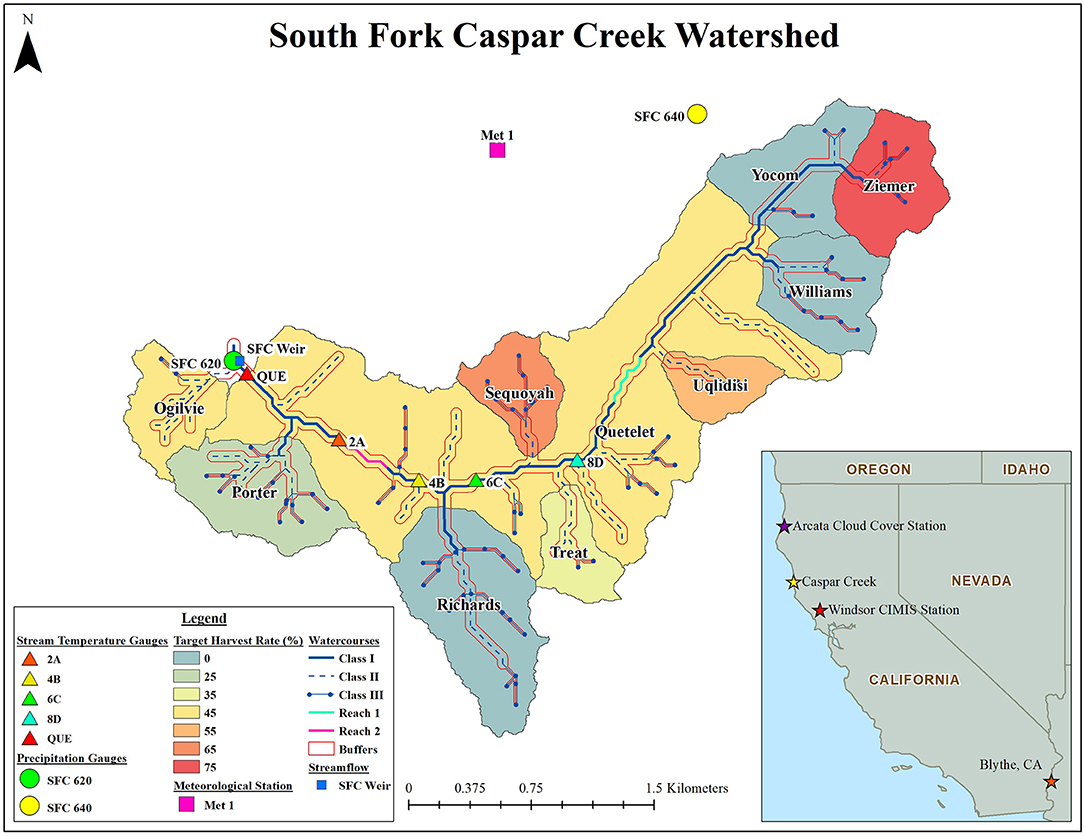
Figure 1. Map depicting the South Fork of Caspar Creek sub-watersheds, stream temperature stations, precipitation stations, meteorological station, weir, watercourse classes, simulated reaches, simulated target harvest rates and where the South Fork of Caspar Creek Watershed is in relation to the Arcata Cloud Cover Station, Windsor CIMIS station and Blythe, CA comparison location. Map data sources: California Department of Forestry and Fire Protection, ESRI USA. The map created used ArcGIS® software by Esri. ArcGIS® is the intellectual property of Esri and are used herein under license. Copyright © Esri. All rights reserved. For more information about Esri® software, please visit www.esri.com.

The time frame for this study utilizes data collected at the South Fork between 2009 and 2016. For variables not collected on site, or those used to fill data gaps, data were used from the California Irrigation Management Information System (CIMIS), a Meso-West meteorological station and the National Centers for Environmental Information (NCEI) Arcata Airport station.

2.2. DHSVM Inputs

DHSVM requires spatial information about the watershed in the form of binary grids created from ArcInfo coverages of elevation, soil type, soil depth, and vegetation type, and connecting arcs (spatially aligned lines) for the stream network and road network. A 30 m DEM was projected from 2 m LiDAR data provided by the U.S. Forest Service Pacific Southwest Research Station (USFS PSW); a pixel size of 30 m was chosen to encompass the stream channel and road widths found in the South Fork. To represent a uniform, second and third-growth coast redwood and Douglas fir forest, based on forest stand data from JDSF, an average tree height of 45 m and leaf area index (LAI) of 7 was utilized (Webb, unpublished data). Similar to Truitt (2018), we made the assumption that LAI is held constant throughout the year because the dominant forest cover is coast redwood and Douglas fir, with relatively low components of hardwoods.

A sub-surface media depth of 5 m was used across the South Fork, based on soil core depths created for sub-surface water studies (Keppeler, 2019). A soil depth of 1.8 m was used based on maximum depth of soil in the watershed (Soil Survey Staff, N. R. C. S. United States Department of Agriculture); from 1.8 to 5.0 m, depth was considered weathered bedrock and below 5 m depth was assumed to be bedrock. The a priori soil parameters used in DHSVM were derived from soil hydraulic properties measured in the nearby North Fork of Caspar Creek by Carr et al. (2014) (Table 1). A variety of contributing areas were evaluated to develop the stream network; a 10,000 m² contributing area provided the best simulation of stream segment maps used by JDSF. This resulted in 150 individual stream segments for streamflow routing, ranging in length from 30 to 740 m, with an average segment length of 123 m.

TABLE 1

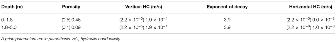
Table 1. A priori and calibrated parameters for the South Fork 2011–2016 HY.

DHSVM explicitly solves the water and energy balance at the grid level (30 m) for simulating the physical processes of canopy interception, evapotranspiration, surface, and subsurface runoff generation driven by climate and geospatial input. When used in conjunction with RBM, DHSVM uses a riparian shading module that simulates the effects of the riparian shading on the energy budget. DHSVM provides key inputs to RBM such as air temperature, downward short- and long-wave radiation, vapor pressure, wind speed, and inflows and outflows for each river segment, which are aggregated as the length-weighted average of the 30 m grids that intercept a stream segment (Sun et al., 2015). RBM uses these inputs, in a separate modeling effort, to simulate stream temperature at 3-h time increments for each of the 150 stream segments.

2.2.1. Meteorological Forcing Files

Meteorological forcing files at a 3-h timestep for air temperature (°C), wind speed (m/s), relative humidity (%), incoming short and long-wave radiation (W/m²), and precipitation (m) were used from August 2009 to September 2016. Fifteen minute interval data from the South Fork meteorological station and precipitation collected at SFC 620 and SFC 640 were converted to a 3-h timestep to be compatible with DHSVM-RBM. To most accurately represent the spatial variation of rainfall, the location of the meteorological station, MET 1 (39 21', 00” N, −123 44' 20” W), and the two precipitation stations, SFC 620 (39 20' 29”, −123 45' 13”) and SFC 640 (39 21' 05”, −123 43' 41”), within the experimental watershed were utilized (Figure 1). Incoming shortwave radiation collected by the CIMIS Windsor Station 103 (Figure 1), was used to estimate the amount of shortwave radiation reaching the site (California Department of Water Resources, 2019) and the Prata (1996) algorithm, coupled with the Unsworth and Monteith (1975) cloud cover correction, were used to calculate incoming long-wave solar radiation, based on Flerchinger et al. (2009) and Wu et al. (2012).

Of the 62,832 total hours between August 1, 2009 and September 30, 2016, 2,038 h of the Caspar Creek Watershed collected meteorological data (3.2%) were missing; gaps lasting <48 h were filled using the average of adjacent readings or directly from corresponding hours (i.e., 9:00 and 9:00 a.m.) within a 5 day time period. If direct readings were substituted, data with similar precipitation patterns were used. Four larger gaps (82, 351, 450, and 934 h) were filled using data from the MESO-West McGuires (MCGC1) Station, located ~11 km further inland than the South Fork of Caspar Creek and residing at 191 m of elevation (39 21' 8”, −123 35' 46”) [Iowa Environmental Mesonet (IEM), 2019]. For 40 recordings (0.06%) of CIMIS shortwave solar radiation data, the average of the surrounding 2 h or direct readings from the corresponding hour during the day before or after were used. Lastly, 18,377 h (29.2%) of cloud cover data, listed as obstructed or left blank, were filled by matching the two surrounding hours, if the same (i.e., clear and clear), or linearly interpolated if different (i.e., between clear and broken).

2.3. RBM Inputs

The RBM model was used to simulate historical stream temperatures in the South Fork by solving time dependent equations for the conservation of thermal energy between the air-water interface. Initial upstream temperatures (hereafter referred to as Mohseni Parameters), stream speed and depth (hereafter referred to as Leopold Parameters), solar radiation, net longwave radiation, sensible heat flux, latent heat flux, groundwater, and advected heat from adjacent tributary segments were used to track water parcels through the river basin and determine temperatures at points along the stream network. DHSVM's stream network was used by RBM to establish the topology for its numerical solution, and stream segment connectivity was used to define the network topology for RBM's particle tracking scheme (Lee et al., 2020). Vegetation height, buffer width, a monthly extinction coefficient, percent overhanging vegetation, canopy bank distance, and channel width were manipulated for each stream segment. For a detailed description of the calculations used in RBM, please refer to Yearsley (2009, 2012) and Sun et al. (2015).

2.3.1. Mohseni Parameters

Four stream temperature and micro-climate gauges (Figure 1), managed by CDFW, were used to estimate parameters used by RBM for initial headwater stream temperatures, due to their close proximity between air and stream temperature gauges. A Mahalanobis distance of 2.448 was used to exclude outliers, and a lambda value of 33.3 was used for the smoothing curve on all gauges to determine the air temperature (°C) at the steepest slope following the inflection point (β) and the angle of trend line at that point (θ). These values were then used in Equations (1), (2), and (3) and final parameters were determined by incrementally adjusting the Mohseni and Leopold variables to find those that resulted in stream temperature estimates closest to measured readings at the outlet of the mainstem (station QUE). A α of 13.5°C, γ of 0.2, β of 10.5°C, μ of 4.0°C, and λ of 0.04 were the final Mohseni variables used; values for each of the individual CDFW stations can be found in (Ridgeway, 2019):

$\begin{array}{ll}{T}_s=\mu +\frac{\alpha -\mu }{1+e^{\gamma (\beta -T_{smooth})}}& (1)\end{array}$

$\begin{array}{ll}\gamma =\frac{4tan\theta }{\alpha -\mu }& (2)\end{array}$

$\begin{array}{ll}{T}_{smooth}=\lambda *T_{air}(t)+(1-\lambda )*T_{air}(t-1)& (3)\end{array}$

where: T_s is the simulated stream temperature, μ is the estimated minimum stream temperature, T_smooth is the smoothed air temperature, α is the maximum actual stream temperature, γ is a measure of the steepest slope of the function, β is the air temperature at the inflection point, γ is a function of the slope tanθ at said point of inflection and the value of λ is determined by the highest possible correlation coefficient between smoothed air temperature and measured water temperature.

2.3.2. Leopold Parameters

RBM uses coefficients based on Leopold and Maddock (1953), which relate velocity and depth to river discharge to establish hydraulic characteristics for each stream segment or the entire watershed. Because these equations are constant in time, RBM also allows for minimum stream speed and depth. A 2 m LiDAR DEM was used to estimate the cross sectional area of eight individual cross-sections in the South Fork. A historical weir-stage to cross sectional area relationship was used to estimate the stage at each of the cross sections, which was then matched to the corresponding average discharge of each cross section using 1996–2016 historical streamflow data from the South Fork Caspar Creek Weir (Figure 1; Richardson et al., 2019). Velocity was then back calculated, resulting in depth and velocity to stream discharge relationships. Final Leopold parameters for velocity (m³/s) were a coefficient of 0.08, exponent of 0.003 and minimum of 0.007; final parameters for depth (m) were a coefficient of 0.009, exponent of 0.2 and minimum of 0.15.

$\begin{array}{ll}D=a{Q}^b& (4)\end{array}$

$\begin{array}{ll}v=c{Q}^d& (5)\end{array}$

where: D is depth, v is velocity, Q is discharge and a, b, c, and d are empirical constants determined from discharge rating curves.

2.3.3. Riparian Shading

Tree height (m), buffer width (m), monthly extinction coefficient (similar to LAI), overhang coefficient (%), canopy bank distance (m) and channel width (m) can be modified segment by segment in RBM. Riparian characteristics used in the initial pre-harvest simulation are outlined in Table 2. Buffer widths were based on California FPR watercourse classes, with Class I (fish bearing) watercourses at 46 m and Class II non-fish bearing watercourses with aquatic life at 30 m buffers (Figure 1). A limitation to the study was that RBM does not allow for the creation of varying widths of different protection or canopy level, as is often prescribed in forest BMPs or regulations. Tree height was estimated from LiDAR data within 46 m of watercourses and an average monthly extinction coefficient for Douglas-fir was used based on Thomas and Winner (2011). As with the LAI used in DHSVM, we made the assumption that the monthly extinction coefficient held constant throughout the year due to the dominant species of coast redwood and Douglas fir, with minor components of hardwoods. The overhang coefficient was based on the mean percent canopy density for the South Fork (California Department of Fish and Wildlife, 2006) and based on the high mean percent canopy density of the South Fork, the monthly extinction coefficient was also held constant along all stream classes (Table 2).

TABLE 2

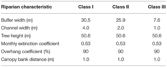
Table 2. Watercouse buffer area characteristics used for initial, second and third-growth conditions along fish bearing watercourses (Class I), non-fish aquatic life supporting watercourses (Class II), and non-aquatic life supporting watercourses (Class III).

2.4. Model Calibration

2.4.1. DHSVM

DHSVM was run for the 2010–2016 hydrologic years (HY) at a 3 h timestep; the HY at Caspar Creek runs from August 1st to July 31st. The model was calibrated during the 2011–2013 HY and verified for the 2014–2016 HY. The 2010 HY was used as a spin-up period to equilibrate the initial water balance and calibration was based on fit to measured streamflow at the South Fork Casapar Creek outlet and Richards subwatershed outlet (Figure 1).

Four sensitive soil hydraulic parameters were adjusted to calibrate the model: (1) lateral hydraulic conductivity, (2) exponent of decay (an exponent of the natural logarithm describing the decrease in hydraulic conductivity by depth of soil), (3) porosity of the soil matrix, and (4) vertical hydraulic conductivity (Surfleet et al., 2010, 2011). These four parameters, and the range of values for each parameter selected, were based on preliminary model trials that demonstrated competence at achieving model fit to measured streamflow.

Statistical fit of the simulated to measured streamflow time series was evaluated using the Nash Sutcliffe Efficiency (NSE) (Equation 6) and the Relative Efficiency (EREL) (Equation 7; Krause et al., 2005). The NSE is a common measure of goodness-of-fit for hydrologic models, because the use of squared values makes them sensitive to high streamflow events. A NSE equal to 1.0 indicates simulated values perfectly match measured values and an NSE ≤ 0 suggest simulated values are worse than the measured mean. The EREL value modifies the NSE as relative deviations, adjusting model fit based on size of event, and thus better reflecting fit of the entire series and reducing the influence of the absolute differences during high flows (Surfleet et al., 2012). As a result, EREL values are more sensitive to systematic over- or under-prediction, particularly during low flow conditions (Krause et al., 2005). This was particularly important to this study, where the primary stream temperature analysis was for summer stream temperatures during low flow periods. Calibration was based on achieving high values of EREL metrics (>0.9), while maintaining reasonable NSE values (>0.6).

$\begin{array}{ll}NSE=1-\frac{{\displaystyle \sum _{t=1}^n{(T_{s_t}-T_{a_t})}^2}}{{\displaystyle \sum _{t=1}^n{({\overline{T}}_a-T_{a_t})}^2}}& (6)\end{array}$

$\begin{array}{ll}{E}_{rel}=1-\frac{{\displaystyle \sum _{t=1}^n}{(\frac{O_t-P_t}{O_t})}^2}{{\displaystyle \sum _{t=1}^n}{(\frac{O_t-\overline{O}}{\overline{O}})}^2}& (7)\end{array}$

where T_s is the simulated stream temperature, T_a is the actual stream temperature, O is observed streamflow, P is simulated streamflow, and t = time step.

2.4.2. RBM

For most coastal western US areas, stream temperatures are generally highest during summer months, coinciding when flows are lowest and energy inputs are highest (clear skies). Therefore, similar to Sun et al. (2015), the period of May 1st to September 30th was evaluated to capture this critical time period for aquatic species. The NSE was again used to gauge goodness of fit; and the Root Mean Square Error (RMSE) was used to assess the quality of the fit, where lower RMSE values, within 1°C, indicate a better fit.

$\begin{array}{ll}RMSE=\sqrt{\frac{{\displaystyle \sum _{t=1}^n}{(T_{s_t}-T_{a_t})}^2}{n-4}}& (8)\end{array}$

RBM was calibrated to measured stream temperatures at the South Fork's primary stream temperature station (QUE), located at the outlet of watershed (Figure 1). After allowing a year of model spin up time, the 2011–2013 summer months (May 1st–September 30th) were evaluated as a calibration period and the 2014–2016 summer months were evaluated as a verification period. Aggregated 3-h output was used to calculate the maximum of the 7-day average temperatures (MWAT) and the maximum of the 7-day maximum temperatures (MWMT). Cao et al. (2016) states that although the use of a 3-h timestep has the potential to limit the ability of RBM to capture daily maxima, it does not do so significantly enough to recommend against using RBM output to calculate the MWMT. The running averages were chosen to remove the occasional spike in stream temperature that can be observed in daily maximums and to reduce the uncertainty in model output from evaluating daily values. Additionally, the MWMT provides an indication of prolonged high temperatures (Gravelle and Link, 2007), thus capturing chronic temperature increases. Finally, the MWAT and MWMT are also used by the United States Environmental Protection Agency and other government agencies to identify viable water temperatures for aquatic species, thus making the results of this study applicable to regulatory agencies.

2.5. Modeling Scenarios

Computer modeling allows researchers to evaluate scenarios that may otherwise be unfeasible or pose too high of a risk to the environment to be implemented. Modeling scenarios in this study were developed based on input from an advisory committee including CAL FIRE and USFS PSW Caspar Creek staff. The simulations are broken into three sections: canopy reduction, the 2017–2019 Phase III South Fork harvest and an experimental riparian conversion design.

Initial, second and third-growth parameters used a tree height of 50.6 (m), monthly extinction coefficient (similar to LAI) of 0.53, overhang coefficient of 90% and canopy bank distance of 1.0 (m). A limitation to the study was that RBM cannot differentiate between varying zones or vegetation canopy difference within streamside buffers, as stipulated in California FPR. Therefore, in an attempt to best simulate buffer area reductions according to the California FPR, buffer width and channel width were based on watercourse class and slope (Figure 1) as follows: fish bearing streams (Class I) buffer width 30.5 m, channel width 4.0 m; non-fish aquatic life supporting watercourses (Class II) buffer width 25.9 m, channel width 2.0 m; and non-aquatic life supporting watercourses (Class III) buffer width 7.6 m, channel width 1.0 m (Table 2).

2.5.1. Canopy Reduction

The first set of scenarios decreased tree height, the monthly extinction coefficient and canopy overhang to 80, 65, 50, 25, and 0% of the initial conditions along the riparian buffers. In order to better evaluate the extent of the impact these scenarios had, two extreme scenarios that altered the entire watershed area and buffer areas were also run. These included clearcutting the entire watershed area and treating the watershed area as if it had never been cut (old growth). The vegetation parameters used for the watercourse buffer areas during each scenario are shown in Table 3; buffer width and channel width, based on stream class, remained at the initial conditions for all scenarios (Table 2). Upslope vegetation inputs (non watercourse buffer areas) within DHSVM were modified from the initial conditions for the old growth and clearcut watershed scenarios by adjusting the LAI and height of vegetation across the watershed area. For the old growth scenario, an upslope tree height of 60 m and LAI of 14 were used to reflect a mix of coast redwood and Douglas-fir trees (Berrill and O'Hara, 2007; Thomas and Winner, 2011; Iberle, 2016). For the clearcut watershed scenario, vegetation height was set to 1 m and an LAI of 1 was used to represent understory vegetation remaining following timber harvesting.

TABLE 3

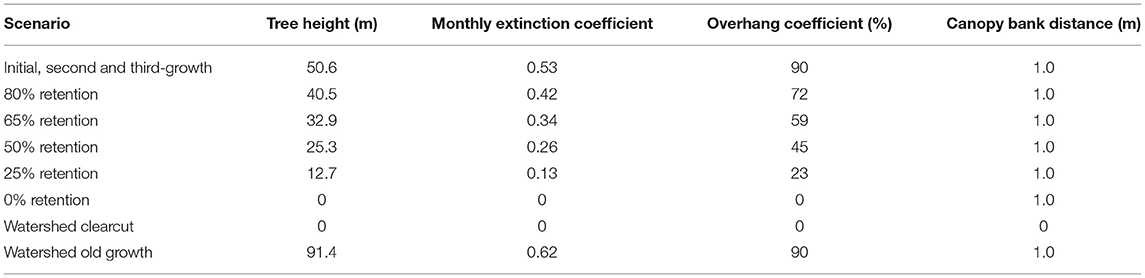
Table 3. Watercourse buffer area characteristics used for each canopy reduction scenario evaluated.

2.5.2. South Fork Caspar Creek Phase III Harvest Scenario

CAL FIRE and the USFS developed an experimental harvest scenario for the South Fork of Caspar Creek (Dymond, 2016), with the goal of quantifying the influence of forest stand density reduction on different watershed processes using the current California FPR. To represent the Phase III 2017–2019 harvest design, each subwatershed was reduced to the appropriate target harvest level by altering the LAI (Figure 1; Table 4). Again, in an attempt to best simulate the California FPR, watercourse buffer reduction rates were determined based on watercourse class. Class I watercourses retained 80% canopy vegetation, Class II watercourses retained 50% canopy and, because California FPR generally do not require canopy retention for non-aquatic life supporting watercourses, 0% canopy vegetation was used for Class III watercourses.

TABLE 4

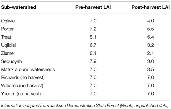
Table 4. Leaf Area Index used in DHSVM simulations of the planned Phase III Harvest of the South Fork of Caspar Creek.

The upslope vegetation inputs for DHSVM were adjusted to reflect the planned reductions in percent basal area completed during the harvest (Figure 1; Table 4). The overstory LAI was changed to reflect the reduced post-harvest overstory (Table 4), using a relationship developed at JDSF for stand density index (SDI) and LAI (Berrill and O'Hara, 2007). Forest inventory data relating basal area with SDI (Webb, unpublished data) allowed LAI to be interpreted for target basal areas in the South Fork harvest.

2.5.3. Riparian Vegetation Conversion

Various studies and agencies have investigated the impact of clearing riparian vegetation in isolated stream reaches for conversion from one dominating vegetative species to another. For example, the Washington State Department of Natural Resources outlines riparian management strategies to restore conifer dominated riparian areas (Bigley and Deisenhofer, 2006). Additional studies in Lassen National Forest seek to restore aspen stands for habitat and ecosystem services (Jones et al., 2013). Furthermore, there has been documented success at releasing suppressed conifers in riparian areas using patch cutting and thinning in parts of Oregon (Emmingham et al., 2000; Maas-Hebner et al., 2005). Therefore, to investigate the impact of practices like these, a scenario clearing two reaches, the first 277 m in length and the second was 322 m in length, was run. Tree height, monthly extinction coefficient, overhang and canopy bank distance for watercourse buffer areas along these segments were set to zero and temperature differences between the segments directly upstream and downstream of the reach were evaluated.

2.6. Sensitivity Analysis

To assess the sensitivity and uncertainty of RBM, three different analyses were completed. The first evaluated the sensitivity to each of the modifiable riparian characteristics. To do this, each variable was incrementally reduced and/or increased, while all other riparian characteristics were held at their initial, second and third-growth values. Modifications used for each variable can be found in Ridgeway (2019).

The second evaluation was done to discern the sensitivity of the air temperature and relative humidity inputs used in the initial DHSVM meteorological files. Air temperature and relative humidity values from CIMIS station #135, Blythe, California, were used because of the consistently high heat and dry conditions in the lower Colorado River Valley. Blythe, California had an average annual air temperature of 21.5°C and relative humidity of 52% from 2011 to 2016. Of the 62,832 total hours, 357 h (0.57%) for air temperature and 344 h (0.54%) for relative humidity had to be filled. Of these gaps, three were longer than 12 h with a maximum gap length of 137 h (5.71 days). Gaps <1 h were filled using the direct readings from the hour before; gaps longer than 1 h were filled with data from the corresponding hour the day before.

The third sensitivity analysis gauged the ability of RBM to predict water temperatures at upstream segments. MWAT and MWMT values calculated from measured data collected at CDFW stations located along various points of the main stem (Figure 1) were compared to water temperatures at the nearest DHSVM-RBM segments simulated without altering the calibration parameters used in all other analyses.

3. Results

3.1. DHSVM

The EREL values for the South Fork during the calibration period were 0.93 and during the validation period were 0.87. The NSE values for both the calibration and validation period in the South Fork were 0.79. In the smaller Richards subwatershed, the EREL during the calibration period was 0.95 and during the validation period was 0.94. The NSE values for this subwatershed were 0.65 during the calibration period and 0.68 during the validation period. Overall, the EREL statistic showed better fit of the simulated streamflow to measured flow, compared to the NSE. Additional hydrograph comparisons illustrating simulated to measured streamflow of the South Fork are included in Figure 2. The visual indications from the model hydrographs indicate DHSVM fit measured streamflow with NSE and EREL statistics ≥ 0.74 and 0.87, respectively, for both the calibration and validation time period (Figure 2). Calibration of DHSVM focused on maximizing the EREL, a metric that is sensitive to streamflows around the mean value, thus providing a better indicator of fit of summer lowflow than the NSE. The mean summer time streamflow for South Fork Caspar Creek for 2011–2015 HY was 6.0 l/s while DHSVM simulated 4.8 l/s for the same period, slightly under-estimating summer time streamflow by on average 1.2 l/s. The South Fork Caspar Creek mean summer time streamflow predicted by DHSVM when the entire watershed was projected to be clearcut increased to 8.7 l/s; an 82% increase over the simulated pre-harvest summer time streamflow.

FIGURE 2

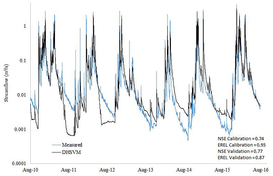
Figure 2. Comparison of streamflow simulated by DHSVM and measured streamflow at the South Fork of Caspar Creek weir HY 2011–2016 and model fit statistics for the calibration period, 2011–2013 HY, and the validation period, 2014–2016 HY.

3.2. RBM

Overall, RBM simulated stream temperatures resulted in NSE values of 0.50 and 0.61 for the calibration and verification periods, respectively (Figure 3). When aggregated, MWAT NSE values increased (0.69 for calibration and 0.65 for verification), while MWMT values increased during the calibration period, but decreased for the verification period (0.73 and 0.34, respectively). RMSE values ranged between 0.68 and 1.01°C. Comparing measured and simulated MWAT results for each year, simulations for 2015 were the closest to measured MWAT values (−0.18°C difference) and having no difference between measured and simulated MWMT values. Simulations for 2011 resulted in the largest difference, with a 1.04°C difference between MWAT values and a 0.82°C difference between MWMT values. Figure 3 exhibits the best fit simulated results to measured stream temperatures at the QUE station for the entire simulated time frame; NSE and RMSE values are included within the time series plots: (Figure 3A) hourly stream temperature (Figure 3B) MWAT, and (Figure 3C) MWMT. Calculated MWAT and MWMT values for measured and simulated results between May and September for each of the 2011–2016 hydrologic years can be found in Ridgeway (2019).

FIGURE 3

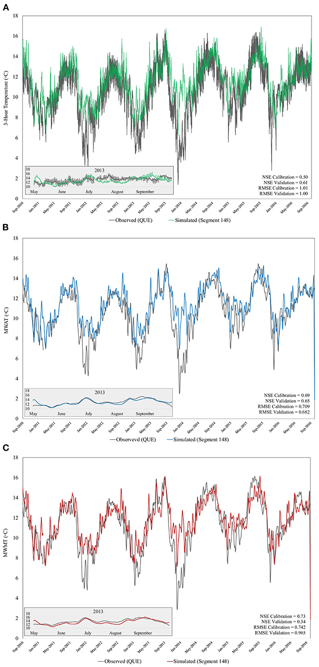
Figure 3. (A) Measured and simulated stream temperatures at a 3 h timestep for the outlet of the South Fork and (B) resulting MWAT values and (C) resulting MWMT values for the measured and simulated stream temperatures. The model was calibrated to the summer months (May 1st–September 30th) 2011–2013, and validated during the summer months of 2014–2016. Inserted plates in each figure show a close-up of one summer time period, May–September 2013.

With the 3-h aggregated output, RBM was not able to fully capture diurnal fluctuations for Caspar Creek. For all three calibration summaries, a greater deviation between simulated and measured values occurred for the winter temperatures (Figure 3). The inserted plates within Figures 3A–C illustrate the May–September 2013 time period; at this scale, the fit of the 3-h time series (insert in Figure 3A) was considerably improved once the MWAT and MWMT were determined (inserts in Figures 3B,C). MWMT peak summer temperatures were estimated more accurately later in the season and during the verification period initial MWMT peak summer temperatures were underestimated. However, RBM was able to more accurately predict these phases for the MWAT.

3.3. Sensitivity Analysis

To evaluate the impact that each of the modifiable RBM vegetation characteristics has on stream temperature, a sensitivity analysis was also done at the QUE stream gauge location (Figure 4). Overall, reducing tree height or the monthly extinction coefficient to zero had a similar effect, with an average increase of 1.51°C for MWAT and 4.48°C for MWMT (Figures 4A,B). RBM predicted lower MWAT and MWMT values when the overhang coefficient was reduced to 50% of initial conditions, compared to when it was reduced to 0% of initial conditions; however, these differences were on average 0.01°C different for MWAT values and 0.07°C different for MWMT values (Figure 4C). Varying the buffer width and canopy bank distance resulted in the same average changes (Figures 4D,E), with an average change of 0.09°C above initial conditions for the MWAT and an average change above initial conditions of 0.34°C for the MWMT. For channel width, the average change above initial conditions for MWAT was 0.10°C and the average change above initial conditions for MWMT was 0.47°C (Figure 4F).

FIGURE 4

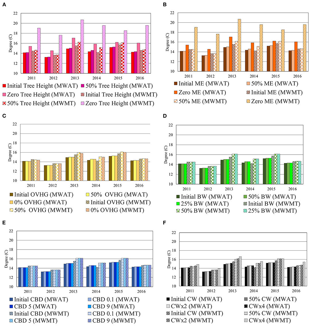
Figure 4. Modeled temperature responses to changes in (A) tree height, (B) monthly extinction coefficient, (C) overhang coefficient, (D) buffer width, (E) canopy bank distance, and (F) channel width, to assess model sensitivity. Bars that are solid represent MWAT results, while bars that are the same color but with strips, represent the MWMT results for that same reduced or increased value.

To evaluate the sensitivity of air temperature and relative humidity, inputs from the Blythe, CA CIMIS station were substituted into the initial meterological forcing files, and riparian vegetation was reduced along all stream segments. In the initial South Fork files, air temperature averaged 13.9°C and relative humidity averaged 78.7% between May and September; during the same time period, Blythe, CA air temperature averaged 29.3°C and relative humidity averaged 49.2%. Year to year variation was low for results using the Blythe, CA data and, on average, increased MWAT values by 3.61°C (range: 2.72–4.96°C) and MWMT values by 3.95°C (range: 3.02–5.61°C; Figure 5).

FIGURE 5

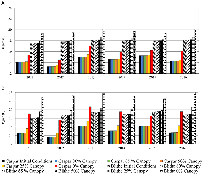
Figure 5. Simulated (A) MWAT and (B) MWMT temperatures using the South Fork of Caspar Creek or Blythe, CA CIMIS air temperature and relative humidity values. Solid lines use Caspar collected values, while dashed lines use Blythe, CA collected values.

Lastly, to evaluate the ability of RBM to predict upstream temperatures, measured temperature readings from CDFW stations 2A, 4B, 6C, and 8D (Figure 1) were compared to simulated temperatures at the closest corresponding RBM segment. RBM did not accurately capture the decreasing trend in MWAT going up the stream network, instead predicting a consistent MWAT trend (Figure 6A). For MWMT results, RBM over estimated upstream temperatures (2A, 4B, 6C, and 8D) and, although not nearly as much as in measured temperatures, captured the decreasing trend between stations 2A, 4B, and 6C (Figure 6B).

FIGURE 6

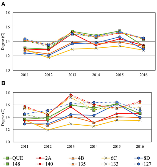
Figure 6. Simulated and measured (A) MWAT and (B) MWMT temperatures for stream temperature stations located throughout the South Fork stream network. Solid lines represent data collected at Caspar Creek (Figure 1), while dashed lines of the same color represent data produced from the corresponding, modeled stream segment.

3.4. Modeling Scenarios

3.4.1. Canopy Reduction

Buffer canopy cover was reduced along only Class I watercourses (Figure 7), and then again along all three watercourse classes (Figure 8). This provided an evaluation of level of canopy cover in the streamside buffer that should be retained to moderate stream temperature increases. The MWAT (Figures 7A, 8A) and MWMT (Figures 7B, 8B) were plotted for each year; solid lines represent when canopy cover was reduced within the buffer and dotted lines represent scenarios where both the buffer and watershed canopy cover were modified (clearcut, old growth).

FIGURE 7

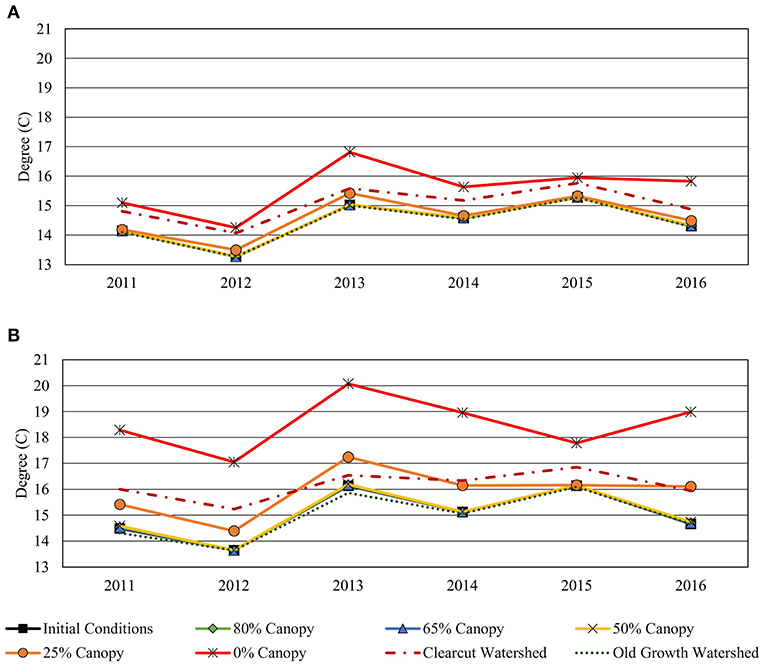
Figure 7. Simulated (A) MWAT and (B) MWMT temperature results for the South Fork mainstem outlet when reducing canopy cover in only Class I watercourses. Solid lines use pre-harvest, second and third-growth vegetation conditions across the watershed, with varying canopy cover in the buffer areas. Dashed lines alter both the watershed and buffer area vegetation.

FIGURE 8

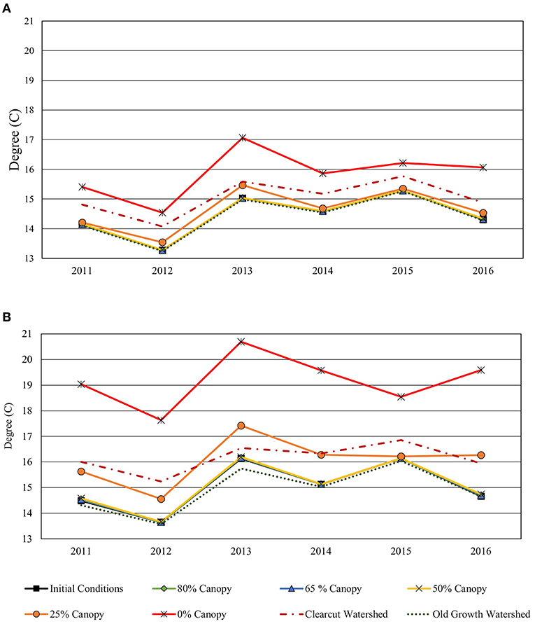
Figure 8. Simulated (A) MWAT and (B) MWMT temperature results for the South Fork mainstem outlet when reducing canopy cover in all stream segments. Solid lines use pre-harvest, second and third-growth vegetation conditions across the watershed, with varying canopy cover in the buffer areas. Dashed lines alter both the watershed and buffer area vegetation.

When altering only Class I watercourse (fish bearing stream) buffers, changes >0.04°C did not occur until riparian conditions were reduced to 25% of the initial, second and third-growth conditions (Figures 7, 8). At this reduction level, the change in MWAT values above initial, second and third-growth conditions ranged from 0.04 to 0.40°C and averaged 0.16°C across the 6 years evaluated. At 0% riparian cover, which simulates clearcutting all Class I watercourse buffers, the increase in MWAT values ranged from 0.67 to 1.79°C, with an average increase of 1.16°C. There was a wider range of increases in temperature above initial conditions when evaluating MWMT results for the 25% retention level, with a range of 0.02–1.45°C and an average of 0.88°C above initial conditions. At the 0% retention level, the increase in MWMT values ranged from 1.64 to 4.33°C and averaged 3.49°C.

There was a larger increase in MWAT and MWMT temperatures when all stream segments had canopy reductions (Figure 8) compared to only Class I watercourses (Figure 7). Changes >0.04°C were again not detected until the 25 and 0% scenarios occurred. At the 25% retention level, MWAT increases ranged from 0.07 to 0.44°C and averaged 0.19°C, while MWMT increases ranged from 0.07 to 1.61°C and averaged 1.03°C. For the 0% reduction scenario, MWAT increases ranged from 0.93 to 2.03°C and averaged 1.42°C, whereas MWMT increases ranged from 2.40 to 4.92°C and averaged 4.14°C.

The results for the old growth and clearcut scenarios were the same whether only Class I (Figure 7) or all watercourses (Figure 8) were modified, because of their affect on the entire watershed. For the clearcut scenario, MWAT values ranged between 0.49 and 0.80°C above initial, second and third-growth values and averaged 0.61°C. MWMT increases ranged from 0.40 to 1.59°C and were on average 1.12°C above initial conditions. For the old growth scenario, MWAT values decreased below initial condition values between 0.01 and 0.04°C, with an average decrease of 0.02°C. MWMT values decreased between 0.01 and 0.27°C, and averaged a 0.10°C decrease. The average change in MWAT and MWMT temperatures when modifying all watercourse classes was graphed for each reduction scenario (Figure 9), which shows the largest difference occurred when the buffer was reduced to 0% canopy, with a 1.42°C change in the MWAT and a 4.14°C change in the MWMT.

FIGURE 9

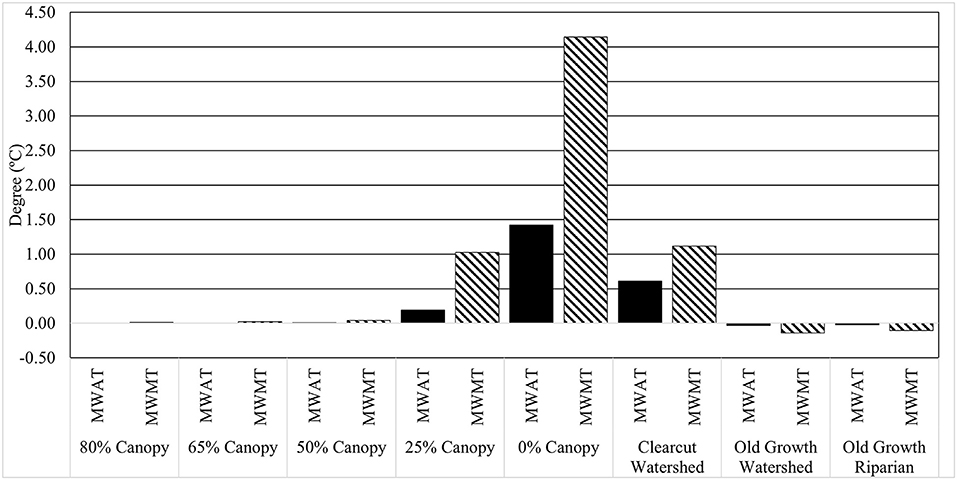
Figure 9. Average MWAT and MWMT temperature (°C) differences between each canopy reduction scenario when all stream segments were reduced and initial, second and third-growth conditions.

3.4.2. South Fork Caspar Creek Phase III Harvest Scenario

For the Phase III harvest scenario, the difference between yearly MWAT and MWMT values for pre and post harvest conditions are graphed in Figure 10. On average, there was a 0.11°C increase in MWAT values and a 0.32°C increase in MWMT values. From year to year, MWMT values varied more than MWAT values (MWAT: 0.10–0.12°C; MWMT: 0.14–0.53°C). The larger difference for HY 2013 is hypothesized to be a result of the spikes in both observed and simulated water temperatures that year, and because average air temperatures between May and September were the third highest (14.2°C) and precipitation was the second lowest (0.86 m measured at SFC 620 during the HY) for 2013.

FIGURE 10

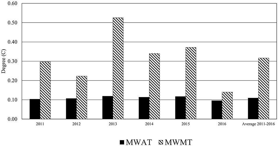
Figure 10. Temperature (°C) differences between MWAT and MWMT values for pre and post harvest conditions.

3.4.3. Riparian Vegetation Conversion

When no vegetation change occurred, RBM predicted a decrease in temperatures between the upper and lower ends of the first reach (−0.01°C change in the MWAT and −0.31°C change in the MWMT), but an increase in water temperature between the upper and lower ends of the second reach (0.01°C change in the MWAT and 0.12°C change in the MWMT). When simulating the clearing of riparian vegetation along these reaches, an increase of 0.72°C in the MWAT and 1.88°C in the MWMT occurred along the first reach, and a larger increase of 0.86°C in the MWAT and 2.87°C in the MWMT occurred along the second reach (Figure 11).

FIGURE 11

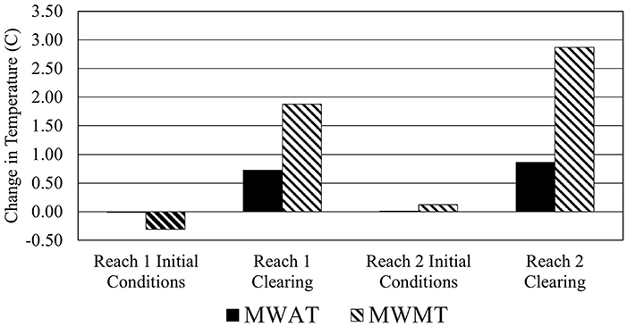
Figure 11. Temperature (°C) difference when clearing isolated stream reaches to simulate converting alder dominated riparian zones to conifer dominated riparian zones.

4. Discussion

4.1. RBM Calibration

Calibration results for the South Fork of Caspar Creek were in line with those of other studies using RBM. Brennan (2015) obtained a combined NSE value of 0.721 using VIC-RBM on the Connecticut River. Truitt (2018) found NSE values for the South, North and Middle forks of the Nooksack River Basin in Washington State to be 0.89, 0.86, and 0.64, respectively. Sun et al. (2015) calibrated RBM to an NSE of 0.90 for the lowest streamflow quartile and estimated the largest differences between measured and simulated temperatures during winter (overestimating measured readings). When evaluating potential dam removal, Perry et al. (2011) reported RMSE values between 0.8 and 1.5°C for the calibration period and 0.8–1.4°C for the verification period. Lastly, RMSE values ranged between 0.63 and 1.92°C, with similarly lower model performance in the verification period compared to the calibration period, for 12 basins in Cao et al. (2016). Therefore, although the South Fork's calibration results were on the lower spectrum, it suggests that RBM estimations were within the precision of other RBM applications.

Most studies attribute uncertainty in model results to estimations of the amount and timing of meltwater inputs. For the South Fork, uncertainty in both streamflow and stream temperatures may be attributed to the inability to simulate changes in groundwater inputs. Additionally, discrepancies may be due to uncertainty in the meteorological forcing files, coefficients used to estimate river hydraulic properties (Leopold coefficients), the use of simulated flows (DHSVM), that riparian vegetation was assumed to be uniform on both sides of the stream network and has no effect on streamflow, that turbidity influences on solar gain and fog drip known to occur at Caspar Creek (Henry, 1998) were not taken into account and that there may be potential effects of microclimate differences throughout the watershed. Estimating water temperature in a system with a measurement device is known to introduce an additional degree of uncertainty from the measurement device itself (Yearsley, 2009). Arismendi et al. (2014) concluded that the Mohseni model does not accurately predict stream temperatures over long periods, or work well to extrapolate future predictions due to the non-stationary relationship between air and stream temperatures over time. This, along with the need to significantly reduce the Mohseni variables, may also be contributing to the discrepancies. Lastly, general data collection errors for both input and comparison data may be adding to differences between model simulations and measured readings.

4.2. Sensitivity Analysis

Each adjustable riparian variable for RBM was reduced and/or increased to assess their sensitivity in the model. Overall, tree height and monthly extinction coefficient were shown to be the most influential. These results agree with those of DeWalle (2010), who found buffer height and extinction coefficient to be crucial to stream shading using a model developed to predict the transmission of potential solar beam radiation. DeWalle (2010) suggests that to maximize stream shading, emphasis should be placed on promoting dense, tall riparian areas, as opposed to focusing on wider buffer widths and for East-West streams (Caspar's orientation), buffer widths above 6–7 m do not provide any additional shading due to shifts in solar beam pathway from the sides to the tops of the buffers. Both of these findings can be supported by the findings using RBM in the South Fork.

Consistency between the increases in MWAT and MWMT values, when substituting in Blythe, California air temperature and relative humidity values, support that stream temperature changes were largely attributed to the modifications of downward solar radiation through topography and riparian vegetation. Additionally, they show that on a year to year basis, Caspar Creek had a more variable meteorology than other regions- cautioning that these results only be applied to similar maritime environments. That said, based on Welsh et al. (2004)'s findings, the 3.5–4.0°C increase across all canopy cover scenarios for both MWAT and MWMT when substituting in Blythe data (Figure 5), suggests that, if air temperatures rise significantly, there may be a reduction in juvenile coho salmon presence. However, the difference between Blythe and South Fork air temperatures (15.4°C on average) was higher than the 1.5°C increase the Intergovernmental Panel on Climate Change (IPCC, 2018) estimates global warming to reach between 2030 and 2052, suggesting current riparian shade requirements may be enough to moderate for fish presence.

The primary limitation to this study was the inability to differentiate between varying zones (e.g., core, inner, and outer) or vegetation canopy difference within streamside buffers. This required simplification of the true design of buffer area protection zones used in many forest BMPs and regulations. Conjointly, the inaccuracies in predicting daily extremes (i.e., diurnal fluctuations) limit the ability to predict the results of extreme warmer and cooler temperatures that can impact aquatic species adapted to cold water environments.

4.3. Modeling Scenarios

4.3.1. Canopy Reduction

Overall, the differences in MWAT and MWMT values for the initial second and third-growth riparian conditions, compared to the 25 and 0% canopy cover reduction scenarios, as well as the old growth scenario, highlight the importance of riparian vegetation in moderating stream temperatures. The old growth scenario modeled in this study averaged 0.02°C for MWAT and 0.10°C for MWMT lower than the initial, second and third-growth results. These findings were similar to those comparing urban riparian vegetation to historical forested vegetation in the Mercer Creek watershed (Sun et al., 2015) and Puget Sound Basin (Cao et al., 2016). For the basin wide scenarios in these studies, Sun et al. (2015) saw an average difference in annual peak stream temperatures at the basin outlet of about 4°C and Cao et al. (2016) saw changes in summer temperature at various basin outlets range between −0.12 and 0.19°C. For Cao et al. (2016), the changes in summer temperatures for the riparian vegetation only scenarios ranged from 0.19 to 1.75°C.

RBM predicted increases on average of 4.14°C above baseline conditions at the 0% canopy retention level. These findings were similar to those of Moore et al. (2005), who observed an ~5°C increase in daily maximum temperatures downstream of a clearcut harvest in a coastal headwater stream in British Columbia. Johnson and Jones (2000) saw an even larger increase, a 7°C increase in daily maximum stream temperatures in the western Cascades of Oregon, attributed to influences of conductive heat transfer from a dark bedrock substrate. Predictions when clearcutting the entire watershed, both upslope and streamside buffer vegetation, in this study produced a lower increase in MWAT and MWMT values than simulations with 0% canopy retention. The South Fork Caspar Creek mean summer time streamflow, predicted by DHSVM if the entire watershed was clearcut, increased from 4.8 to 8.7 l/s, an 82% increase over the pre-harvest streamflow. This was attributed to the decrease in ET and subsequent increase in water yield following the basin-wide clearcut that is consistent with globally recognized effects of harvesting (Buttle, 2011). We attribute the increase in summer streamflow, from the removal of all forest vegetation in the modeling, to dilute the increased heat inputs from removal of stream shade.

The RBM simulations for the South Fork indicated only 1 year, with 0% canopy retention, exceeded the MWAT threshold (16.7°C) proposed by Welsh et al. (2004) when studying juvenile coho salmon presence in the Mattole River. However, all but one of the MWMT estimates, at the 0% canopy retention, exceeded the suggested 18.0°C threshold suggested by Welsh et al. (2004). It should be cautioned however, that Hines and Ambrose (2000) strongly recommend against the use of a single value to predict complex phenomenon such as salmonid presence.

4.3.2. South Fork Caspar Creek Phase III Harvest Scenario

When simulating the South Fork Caspar Creek Phase III harvest with California FPR buffer widths, the MWAT increased on average by 0.11°C and the MWMT increased on average by 0.32°C for MWMT increases. This suggest a slight increase may occur for both MWAT and MWMT stream temperatures, but were under the maximum 2.78°C increase allowed under California state regulations for cold water habitat. The average MWAT and MWMT estimates (14.5 and 15.4°C, respectively) were also below thresholds for coho salmon and steelhead species (Eaton et al., 1995; McCullough et al., 2001; Welsh et al., 2004; Sloat and Osterback, 2013). Additionally, temperature changes were lower for the harvest scenario than the ≤ 50% canopy retention, suggesting California FPR requirements successfully mitigate impacts to stream temperature.

The average change in stream temperatures following the Phase III harvest were similar to those of Cao et al. (2016) who found that basin-wide land cover changes affected stream temperature <0.2°C in both summer and winter seasons using DHSVM-RBM. Although, stream temperature was not collected after selective harvesting occurred in the South Fork in the early 1970s, summer maximum and average daily high temperatures in an uncut tributary basin for the North Fork were 2.8°C lower than those in the clearcut mainstem that used buffer strips on both sides (Cafferata, 1990). Further down the mainstem of the North Fork, summer maximums were found to be 15.6°C, suggesting that waters were diluted with cooler water from three uncut tributaries below the clearcut. Therefore, the findings of this study were within an expected range of post harvest results and suggests impacts of a decrease in riparian cover are mitigated due to the location of QUE at the end of the mainstem, the mix of harvest rates and increases in baseflow volume following a loss of evapotranspiration.

4.3.3. Riparian Vegetation Conversion

In 1967, after a road was built in the South Fork of Caspar Creek riparian zone, researchers recorded increases of 1.7–2.2°C in areas “where water flowed from shaded to open areas” (Cafferata, 1990). Although, it was not noted how long these distances were, the conversion scenario suggest similar findings of an average 0.5°C increase in MWAT values and a 2.5°C increase in MWMT values simulated for 277 and 322 m openings in this study. That said, the sensitivity analysis evaluating the ability to predict upstream temperatures using CDFW stream temperature stations suggest that RBM did not accurately predict temperatures in upstream segments for the South Fork of Caspar Creek. Temperatures for the stream segment immediately following the clearing were back to identical readings of those directly above the clearing, suggesting RBM may be doing little to track water downstream, and instead predicting temperatures directly based on riparian conditions.

4.4. Uncertainty in Modeling Approach

Simulations of stream temperature, using the combination of DHSVM calibrated to two streamflow gauges with output forcing the RBM model, fit the weekly averages of measured stream temperatures within 1.1°C. The weaker performance of the modeling at some locations highlights the importance of accounting for modeling errors and uncertainty. The greatest source of uncertainty in the forcing data for DHSVM-RBM was in the use of solar radiation and cloud cover from sources outside of the South Fork Caspar Creek watershed. Cloud cover negatively affects short wave radiation inputs while positively affecting long wave radiation. We believe the uncertainty presented by the solar radiation forcing was reduced by using generalized output comparing average weekly stream temperatures. Further the measurement of stream temperature can vary greatly along stream segments in small watersheds. The calibration of RBM to point measurements of stream temperature in the South Fork Caspar Creek would not capture this variability. The mismatch in temporal resolution between model simulations (3-h) and measured stream and temperature calibration data collected at finer resolution may result in a greater level of uncertainty. DHSVM hydrologic modeling presents parameter uncertainties and lacks a groundwater component. In the development of RBM it was shown that basin-wide uniform Mohseni parameters (Yearsley, 2009) used to estimate the headwater temperatures present another possible source of error. Because the impact of the error associated with simulated headwater temperature decays as water travels downstream, its impact is generally negligible in large river basins (Lee et al., 2020). However, in small headwater watersheds like the South Fork of Caspar Creek, Yearsley (2012) demonstrated a standard deviation of 2°C in simulated temperatures from the uncertainty in groundwater temperature inputs, which presents uncertainties in model accuracy. The version of RBM used in this study alters heat energy exchange from riparian vegetation by tree height and the overhang coefficient blocking the solar radiance throughout the day. Canopy gaps in the riparian stand across the buffer width were not part of the simulations. Sensitivity analysis showed that changes in width of the riparian area in RBM were sensitive in simulation of stream temperatures. However, this represented a change in the solar inputs by blockage of the solar heat input due to tree height (i.e., solar geometry as the buffer advanced up the canyon sides).

5. Conclusion

Intensive datasets collected at the Caspar Creek Experimental Watersheds allowed for the application of a highly detailed, distributed hydrology-stream temperature model. DHSVM-RBM was calibrated to historical readings to reasonably predict MWAT and MWMT at the outlet of the South Fork of Caspar Creek. Predicted changes in stream temperature were similar to several other studies using RBM at other locations; however, differences in model fit between calibration and verification periods demonstrate some uncertainty in model precision. Model discrepancies were hypothesized to be primarily a result of inaccuracies estimating groundwater inputs, uncertainty in the meteorological forcing files, coefficients used to estimate hydraulic properties and uncertainty in initial headwater temperatures.

RBM did not predict substantial changes in stream temperature until reducing buffer canopy to 25 and 0% retention levels in the South Fork of Caspar Creek, which were well below current California FPR levels. All except 1 year with 0% canopy retention had MWMT estimates that were above recommended temperature thresholds for juvenile coho salmon (Welsh et al., 2004) and state law. RBM estimates that if clearcutting the entire watershed occurs, significant enough increases in water yield mitigated increases in MWAT and MWMT values. A contemporary selective forest harvest, with streamside buffers at 80% canopy cover, resulted in little change in average or maximum stream temperatures. Substitution of climate data from Blythe, California warn of potential impacts to stream temperatures in the South Fork if considerably warmer air temperature and lower relative humidity values occur. Overall, these findings support the work of other modeling efforts stressing the importance of riparian vegetation in moderating stream temperatures.

At this time, we cannot say with certainty that DHSVM-RBM accurately predicts upstream temperatures in the South Fork using a calibration at the outlet of the watershed. Inaccuracies regarding estimations were hypothesized to primarily be due to groundwater inputs, soil macropore flow and varying microclimates. Sensitivity analyses support other modeling efforts in suggesting land managers concentrate on maintaining tall, dense buffers, as opposed to focusing on wider buffer widths. Required buffer width has been shown to be closely related to the orientation of the stream (N-S vs. E-W), which may be significant in these findings and should be further evaluated.

Data Availability Statement

The raw data supporting the conclusions of this article will be made available by the authors, without undue reservation.

Author Contributions

CS conducted the DHSVM modeling. JR conducted the RBM modeling and wrote the manuscript with the contribution of CS. All authors contributed to the article and approved the submitted version.

Funding

This work was supported by funding from the California Department of Forestry and Fire Protection in support of the Caspar Creek Phase III Research, agreement #8CA03637.

Conflict of Interest

The authors declare that the research was conducted in the absence of any commercial or financial relationships that could be construed as a potential conflict of interest.

Acknowledgments

Observed data sets were provided by the Caspar Creek Experimental Watersheds project, which was funded by the USDA Forest Service Pacific Southwest Research Station and the California Department of Forestry and Fire Protection. Additional stream temperature data sets were provided by the California Department of Fish and Wildlife. Thank you to Andrew Adriance, whose optimized model scripts reduced DHSVM model runtime (Adriance, 2018).

References

Adriance, A. (2018). Optimizing the distributed hydrology soil vegetation model for uncertainty assessment with serial, multicore and distributed accelerations (MSc thesis). California Polytechnic State Unviersity, San Luis Obispo, CA, United States.

Google Scholar

Arismendi, I., Safeeq, M., Dunham, J. B., and Johnson, S. L. (2014). Can air temperature be used to project influences of climate change on stream temperature? Environ. Res. Lett. 9:084015. doi: 10.1088/1748-9326/9/8/084015

CrossRef Full Text | Google Scholar

Berrill, J.-P., and O'Hara, K. L. (2007). Patterns of leaf area and growing space efficiency in young even-aged and multiaged coast redwood stands. Can. J. For. Res. 37, 617–626. doi: 10.1139/X06-271

CrossRef Full Text | Google Scholar

Beschta, R. L., Bilby, R. E., Brown, G. W., Holtby, L. B., and Hofstra, T. D. (1987). “Chapter 6: Stream temperature and aquatic habitat,” in Streamside Management: Forestry and Fishery Interactions, Contribution No. 57, eds E. O. Salo and T. W. Cundy (University of Washington; Institute of Forest Resources), 191–232.

Bigley, R., and Deisenhofer, F. (2006). Implementation Procedures for the Habitat Conservation Plan Riparian Forest Restoration Strategy. DNR Scientific Support Section, Olympia, WA.

Brennan, L. (2015). Stream temperature modeling: a modeling comparison for resource managers and climate change analysis (MSc thesis). University of Massachusetts Amherst, Amherst, MA, United States.

Google Scholar

Brown, G. W., and Krygier, J. T. (1970). Effects of clear cutting on stream temperature. Water Resour. Res. 6, 1133–1139. doi: 10.1029/WR006i004p01133

CrossRef Full Text | Google Scholar

Buttle, J. M. (2011). “The effects of forest harvesting on forest hydrology and biogeochemistry,” in Forest Hydrology and Biogeochemisty, Synthesis of Past Research and Future Directions, eds D. F. Levia, D. Carlyle-Moses, and T. Tanaka (Springer), 659–678. doi: 10.1007/978-94-007-1363-5_33

CrossRef Full Text | Google Scholar

Cafferata, P. (1990). Temperature Regimes of Small Streams Along the Mendocino Coast. JDSF Newsletter. Jackson Demonstration State Forest; State of California Dept. of Forestry. No. 29.

Google Scholar

California Department of Fish and Wildlife (2006). Stream Inventory Report: South Fork Caspar Creek. Technical report, The Pacific States Marine Fisheries Commission (PSMFC). California Department of Fish and Wildlife.

California Department of Forestry and Fire Protection (2020). California Forest Practice Rules, Anadromous Salmon Protection Rules. California Department of Forestry and Fire Protection.

California Department of Water Resources (2019). California Irrigation Managment Information System (CIMIS). California Department of Water Resources.

Cao, Q., Sun, N., Yearsley, J., Nijssen, B., and Lettenmaier, D. P. (2016). Climate and land cover effects on the temperature of Puget Sound streams. Hydrol. Process. 30, 2286–2304. doi: 10.1002/hyp.10784

CrossRef Full Text | Google Scholar

Carr, A. E., Loague, K., and Vanderkwaak, J. E. (2014). Hydrologic-response simulations for the north fork of caspar creek: second-growth, clear-cut, new-growth, and cumulative watershed effect scenarios. Hydrol. Process. 28, 1476–1494. doi: 10.1002/hyp.9697

CrossRef Full Text | Google Scholar

Carroll, G. D., Schoenholtz, S. H., Young, B. W., and Dibble, E. D. (2004). Effectiveness of forestry streamside managment zones in the sand-clay hills of Mississippi: early indications. Water Air Soil Pollut. 4, 275–296. doi: 10.1023/B:WAFO.0000012813.94538.c8

CrossRef Full Text | Google Scholar

DeWalle, D. R. (2010). Modeling stream shade: Riparian buffer height and density as important as buffer width. J. Am. Water Resour. Assoc. 46, 323–333. doi: 10.1111/j.1752-1688.2010.00423.x

CrossRef Full Text | Google Scholar

Dugdale, S. J., Hannah, D. M., and Malcolm, I. A. (2017). River temperature modelling: a review of process-based approaches and future directions. Earth Sci. Rev. 175, 97–113. doi: 10.1016/j.earscirev.2017.10.009

CrossRef Full Text | Google Scholar

Dymond, S. F. (2016). Caspar Creek Experimental Watersheds Experiment Three Study Plan: The Influence of Forest Stand Density Reduction on Watershed Processes in the South Fork. Technical report, USDA Forest Service Pacific Southwest Research Station.

Google Scholar

Eaton, J. G., McCormick, J. H., Goodno, B. E., O'Brien, D. G., Stefany, H. G., Hondzo, M., et al. (1995). A field information-based system for estimating fish temperature tolerances. Fisheries. 20, 10–18. doi: 10.1577/1548-8446(1995)020<0010:AFISFE>2.0.CO;2

CrossRef Full Text | Google Scholar

Eliason, E. J., Clark, T. D., Hague, M. J., Hanson, L. M., Gallagher, Z. S., Jeffries, K. M., et al. (2011). Differences in thermal tolerance among Sockeye salmon populations. Science 332, 109–112. doi: 10.1126/science.1199158

PubMed Abstract | CrossRef Full Text | Google Scholar

Emmingham, B., Chan, S., Mikowski, D., Owston, P., and Bishaw, B. (2000). Silviculuture Practices for Riparian Forests in the Oregon Coast Range. Technical report, Forest Research Laboratory, Corvallis, OR.

Google Scholar

Flerchinger, G. N., Xaio, W., Marks, D., Sauer, T. J., and Yu, Q. (2009). Comparison of algorithms for incoming atmospheric long-wave radiation. Water Resour. Res. 45:W03423. doi: 10.1029/2008WR007394

CrossRef Full Text | Google Scholar

Gomi, T., Moore, R. D., and Dhakal, A. S. (2006). Headwater stream temperature response to clear-cut harvesting with different riparian treatments, coastal British Columbia, Canada. Water Resour. Res. 42, 1–11. doi: 10.1029/2005WR004162

CrossRef Full Text | Google Scholar

Gravelle, J. A., and Link, T. E. (2007). Influence of Timber Harvesting on Headwater Peak Stream Temperatures in a Northern Idaho Watershed. Technical report: Forest Science 53(2) copyright by the Society of American Foresters.

Google Scholar

Henry, N. (1998). “Overview of the Caspar Creek watershed study,” in Proceedings of the Conference on Coastal Watersheds: The Caspar Creek Story (Ukiah, CA: Pacific Southwest Research Station), 1–9.

Google Scholar

Hines, D., and Ambrose, J. (2000). Evaluation of Stream Temperatures Based on Observations of Juvenile Coho Salmon in Northern California Streams. Technical report, Campbell Timberladn Management, Inc.; National Marine Fisheries Service.

Google Scholar

Iberle, B. G. (2016). Ninetry-two years of tree growth and death in a second-growth coast redwood forest (MSc thesis). Humboldt State University, Arcata, CA, United States.

Google Scholar

Iowa Environmental Mesonet (IEM) (2019). McGuires Raws (MCGC1) Meterological Station. Iowa Environmental Mesonet (IEM).

IPCC (2018). “Summary for policymakers,” in Global Warming of 1.5 °C. An IPCC Special Report on the Impacts of Global Warming of 1.5 °C Above Pre-Industrial Levels and Related Global Greenhouse Gas Emission Pathways, in the Context of Strengthening the Global Response to the Threat of Climate Change, IPCC, 1–21.

Johnson, S. L., and Jones, J. A. (2000). Stream temperature responses to forest harvest and debris flows in western Cascades, Oregon. Can. J. Fish. Aquat. Sci. 57, 30–39. doi: 10.1139/f00-109

CrossRef Full Text | Google Scholar

Jones, B. E., Krupa, M., and Tate, K. W. (2013). Aquatic ecosystem response to timber harvesting for the purpose of restoring aspen. PLoS ONE 8:e84561. doi: 10.1371/journal.pone.0084561

PubMed Abstract | CrossRef Full Text | Google Scholar

Keppeler, E. (2019). Personal communication on soil auger holes for sub surfacewells May 9, 2019.

Krause, P., Boyle, D. P., and Bäse, F. (2005). Comparison of different efficiency criteria for hydrological model assessment. Adv. Geosci. 5, 89–97. doi: 10.5194/adgeo-5-89-2005

CrossRef Full Text | Google Scholar

Larson, L. L., and Larson, S. L. (1996). Riparian shade and stream temperature: a perspective. Soc. Range Manage. 18, 149–152.

Google Scholar

Lee, S.-Y., Fullerton, A. H., Sun, N., and Torgersen, C. E. (2020). Projecting spatiotemporally explicit effects of climate change on stream temperature: a model comparison and implications for coldwater fishes. J. Hydrol. 588. doi: 10.1016/j.jhydrol.2020.125066

CrossRef Full Text | Google Scholar

Leopold, L. B., and Maddock, T. J. (1953). The Hydraulic Geometry of Stream Channels and Some Physiographic Implications. United States Government Printing Office, Washington, DC. 252. doi: 10.3133/pp252

CrossRef Full Text | Google Scholar

Lynch, J. A., and Corbett, E. S. (1990). Evaluation of Best Management Practices for controlling nonpoint pollution from silvicultural operations. J. Am. Water Resour. Assoc. 26, 41–52. doi: 10.1111/j.1752-1688.1990.tb01349.x

CrossRef Full Text | Google Scholar

Maas-Hebner, K. G., Emmingham, W. H., Larson, D. J., and Chan, S. S. (2005). Establishment and growth of native hardwood and conifer seedlings underplanted in thinned Douglas-fir stands. For. Ecol. Manage. 208, 331–345. doi: 10.1016/j.foreco.2005.01.013

CrossRef Full Text | Google Scholar

Macdonald, J. S., Beaudry, P. G., Macisaac, E. A., and Herunter, H. E. (2003). The effects of forest harvesting and best management practices on streamflow and suspended sediment concentrations during snowmelt in headwater streams in sub-boreal forests of British Columbia, Canada. Can. J. For. Res. 33, 1397–1407. doi: 10.1139/x03-110

CrossRef Full Text | Google Scholar

McCullough, D., Spalding, S., Sturdevant, D., and Hicks, M. (2001). Summary of Technical Literature Examining the Physiological Effects of Temperature on Salmonids. US Environmental Protection Agency, 1–119.

Google Scholar

Moore, R. D., Spittlehouse, D. L., and Story, A. (2005). Riparian microclimate and stream temperature response to forest harvesting: a review. J. Am. Water Resour. Assoc. 41, 813–834. doi: 10.1111/j.1752-1688.2005.tb04465.x

CrossRef Full Text | Google Scholar

Parkyn, S. M., Davies-Colley, R. J., Halliday, N. J., Costley, K. J., and Croker, G. F. (2003). Planted riparian buffer zones in New Zealand: do they live up to expectations? Restor. Ecol. 11, 436–447. doi: 10.1046/j.1526-100X.2003.rec0260.x

CrossRef Full Text | Google Scholar

Patric, J. (1980). Effects of wood products harvest on forest soil and water relations. J. Environ. Qual. 9:73. doi: 10.2134/jeq1980.00472425000900010018x

CrossRef Full Text | Google Scholar

Perry, R. W., Risley, J. C., Brewer, S. J., Jones, E. C., and Rondorf, D. W. (2011). Simulating Daily Water Temperatures of the Klamath River Under Dam Removal and Climate Change Scenarios. U.S. Geological Survey Open-File Report 2011–1243, 78.

Google Scholar

Prata, A. J. (1996). A new long-wave formula for estimating downward clear-sky radiation at the surface. Q. J. R. Meteorol. Soc. 122, 1127–1151. doi: 10.1002/qj.49712253306

CrossRef Full Text | Google Scholar

Quinn, J. M., Steele, G. L., Hickey, C. W., and Vickers, M. L. (1994). Upper thermal tolerances of twelve New Zealand stream invertebrate species. N. Z. J. Mar. Freshw. Res. 28, 391–397. doi: 10.1080/00288330.1994.9516629

CrossRef Full Text | Google Scholar

Rice, R. M., Tilley, F. B., and Datzman, P. A. (1979). A Watershed's Response to Logging and Roads: South Fork of Caspar Creek, California 1967-1976. Technical report, Pacific Southwest Forest and Range Experiment Station, Berkeley, CA.

Google Scholar

Richardson, P. W., Seehafer, J. E., Keppeler, E. T., Sutherland, D. G., and Wagenbrenner, J. W. (2019). Caspar Creek Experimental Watersheds Phase 2 (1985-2017) Data. Fort Collins, CO: Forest Service Research Data Archive. doi: 10.2737/RDS-2020-0018

CrossRef Full Text | Google Scholar

Ridgeway, J. (2019). An analysis of changes in stream temperature due to forest harvest practices using DHSVM-RBM (MSc Thesis). California Polytechnic State University, San Luis Obispo, CA, United States.

Google Scholar

Sloat, M. R., and Osterback, A.-M. K. (2013). Maximum stream temperature and the occurrence, abundance, and behavior of steelhead trout (Oncorhynchus mykiss) in a southern California stream. Can. J. Fish. Aquat. Sci. 70, 64–73. doi: 10.1139/cjfas-2012-0228

CrossRef Full Text | Google Scholar

Soil Survey Staff, N. R. C. S. United States Department of Agriculture. (2019). U.S. General Soil Map (STATSGO2). Soil Survey Staff N. R. C. S. United States Department of Agriculture. (accessed August 02, 2019).

Google Scholar

Sun, N., Yearsley, J., Voisin, N., and Lettenmaier, D. P. (2015). A spatially distributed model for the assessment of land use impacts on stream temperature in small urban watersheds. Hydrol. Process. 29, 2331–2345. doi: 10.1002/hyp.10363

CrossRef Full Text | Google Scholar

Surfleet, C. G., Skaugset, A. E., and McDonnell, J. J. (2010). Uncertainty assessment of forest road modeling with the Distributed Hydrology Soil Vegetation Model (DHSVM). Can. J. For. Res. 40, 1397–1409. doi: 10.1139/X10-079

CrossRef Full Text | Google Scholar

Surfleet, C. G., Skaugset, A. E., and Meadows, M. W. (2011). Road runoff and sediment sampling for determining road sediment yield at the watershed scale. Can. J. For. Res. 41, 1970–1980. doi: 10.1139/x11-104

CrossRef Full Text | Google Scholar

Surfleet, C. G., Tullos, D., Chang, H., and Jung, I.-W. (2012). Selection of hydrologic modeling approaches for climate change assessment: a comparison of model scale and structure. J. Hydrol. 464–465, 233–248. doi: 10.1016/j.jhydrol.2012.07.012

CrossRef Full Text | Google Scholar

Sweeney, B. W., and Newbold, J. D. (2014). Streamside forest buffer width needed to protect stream water quality, habitat, and organisms: a literature review. J. Am. Water Resour. Assoc. 50, 560–584. doi: 10.1111/jawr.12203

CrossRef Full Text | Google Scholar

Thomas, S. C., and Winner, W. E. (2011). Leaf area index of an old-growth Douglas-fir forest estimated from direct structural measurements in the canopy. Can. J. For. Res. 30, 1922–1930. doi: 10.1139/x00-121

CrossRef Full Text | Google Scholar

Truitt, S. E. (2018). Modeling the effects of climate change projections on streamflow in the Nooksack River Basin, Northwest Washington (MSc thesis). Western Washington University, Bellingham, WA, United States.

Google Scholar

Unsworth, M. H., and Monteith, J. (1975). Long-wave radiation at the ground. Q. J. R. Meteorol. Soc. 101, 25–34. doi: 10.1256/smsqj.42703

CrossRef Full Text | Google Scholar

Van Vliet, M. T., Sheffield, J., Wiberg, D., and Wood, E. F. (2016). Impacts of recent drought and warm years on water resources and electricity supply worldwide. Environ. Res. Lett. 11. doi: 10.1088/1748-9326/11/12/124021

CrossRef Full Text | Google Scholar

Van Vliet, M. T. H., Franssen, W. H. P., Yearsley, J. R., Ludwig, F., Haddeland, I., Lettenmaier, D. P., et al. (2013). Global river discharge and water temperature under climate change. Glob. Environ. Change 23, 450–464. doi: 10.1016/j.gloenvcha.2012.11.002

CrossRef Full Text | Google Scholar

Wagenbrenner, J. (2018). Addendum to Caspar Creek Experimental Watersheds Experiment Three Study Plan: The Influence of Forest Stand Density Reduction on Watershed Processes in the South Fork. Technical report, USDA Forest Service Pacific Southwest Research Station.

Google Scholar

Washington State Legislature (1999). Salmon Recovery Act. Revised Code of Washington. Washington State Legislature. doi: 10.2307/40251811

CrossRef Full Text | Google Scholar

Welsh, H. H., Hodgson, G. R., Harvey, B. C., and Roche, M. F. (2004). Distribution of juvenile Coho salmon in relation to water temperatures in tributaries of the Mattole River, California. North Am. J. Fish. Manage. 21, 464–470. doi: 10.1577/1548-8675(2001)021<0464:DOJCSI>2.0.CO;2

CrossRef Full Text | Google Scholar

Wilkerson, E., Hagan, J. M., Siegel, D., and Whitman, A. A. (2006). Effectiveness of different buffer widths for protecting headwater stream temperature in Maine. For. Sci. 52, 221–231.

Google Scholar

Wu, H., Zhang, X., Liang, S., Yang, H., and Zhou, G. (2012). Estimation of clear-sky land surface longwave radiation from MODIS data products by merging multiple models. J. Geophys. Res. Atmos. 117:D22107. doi: 10.1029/2012JD017567

CrossRef Full Text | Google Scholar

Yearsley, J. (2012). A grid-based approach for simulating stream temperature. Water Resour. Res. 48, 1–15. doi: 10.1029/2011WR011515

CrossRef Full Text | Google Scholar

Yearsley, J. R. (2009). A semi-Lagrangian water temperature model for advection-dominated river systems. Water Resour. Res. 45, 1–19. doi: 10.1029/2008WR007629

CrossRef Full Text | Google Scholar

Ziemer, R. R., and Alright, J. S. (1987). “Subsurface pipeflows dynamics of north-coastal California swale system,” in Corvallis Symposium (Arcata, CA), 71–80.

Google Scholar