Water balance for gaged watersheds in the Central Sierra Nevada, California and Nevada, United States

Introduction

Accurate measurements of annual water balance are foundational for predicting how water supplies and ecosystem health in semi-arid regions will respond to a warming climate and prolonged droughts. Determining water balance has traditionally depended on precipitation and streamflow data, with actual evapotranspiration inferred from energy-balance modeling or indirect correlations. We define the annual water balance as:

$P=ET+Q+D+-\mathrm{\Delta }S+R(1)$

where P is annual precipitation, ET is evapotranspiration, Q is discharge, D is diversion, ΔS is change in storage, with positive values representing additions to root-accessible subsurface storage. Diversion refers to water leaving the watershed but not part of measured streamflow (Q), and in this context can include both net subsurface flow out, as well as engineered diversions of streamflow. R is the residual, or imbalance, after accounting for the other terms.

With the advent of high-confidence spatial evapotranspiration estimates driven by a robust relation between satellite-derived estimates of normalized difference vegetation index (NDVI) and point measurements of ET in a variety of vegetation types (Goulden et al., 2012; Goulden and Bales, 2014), it is possible to estimate water balance with high spatial resolution across forested mountain landscapes. In the context of forest management, this approach permits estimation of changes in ET resulting from past treatments and fire (Roche et al., 2018, 2020) and the potential for change from future treatments (Ma et al., 2020). Further, extending the work of Fellows and Goulden (2017), it may be possible to map the spatial variability in the minimum amount of subsurface water storage, thereby identifying areas with greater or lesser drought resistance and/or potential benefit from thinning treatments (Goulden and Bales, 2019; Bales and Dietrich, 2020). This approach is sufficiently mature to examine factors impacting the variability of interannual water balances, from hillslope to basin scales (Bales et al., 2018).

In an era of rapid environmental change and consequent changes to basin hydrology, it is essential that intuitive tools exist that enable land and water managers to respond to those changes in a timely manner. At the same time, there is broad recognition that data-driven empirical watershed models are necessary to inform development and refinement of more physically based models (Avanzi et al., 2020). The above referenced method for estimating ET is easily calculated, has a high spatial resolution (30 m, using Landsat data), and is sufficiently robust to produce reliable estimates of water balance for larger watersheds (Roche et al., 2020). As such, ET estimated in this way appears to be of the same order of accuracy as annual discharge at gauged locations (10–20%; see Supplementary Figure S3 in Roche et al., 2020) and far more accurate than spatial estimates of precipitation in mountain environments (e.g., Lundquist et al., 2019; Cui et al., 2022).

Though foresters and hydrologists have sought to understand the effects of deforestation and afforestation on basin water balances for a long time, these efforts have largely remained in the realm of intensive research efforts that are not sufficiently representative to scale to broader geographic areas. In general, it is understood that removing trees will increase runoff for a period of time, and that forest regrowth decreases runoff (Saksa et al., 2017). The factors that influence this change and how long it lasts remain less well quantified due to variability in treatment type, extent of treatment relative to watershed area above a stream gauge, climate regime, and whether there are follow-up treatments that make it possible to isolate the post-treatment effects of accelerated growth of remaining large trees from regrowth of other vegetation, including young trees (Ma et al., 2020). Given the urgency of addressing forest drought stress, wildfire impacts on water balance, and water availability in the face of climate change, quantifying the effects of accelerating forest fuels treatments on water balance is central to encouraging investment in forest-thinning treatments (Saksa et al., 2020; Tahoe Central Sierra Initiative, 2022).

Key to this study is an examination of the relative change in subsurface water storage between wet and dry years (Klos et al., 2018; O’Geen et al., 2018). In the context of this work, change in subsurface storage (ΔS) is defined as the interannual deficit in P-ET-Q-D, or excess beyond ET and runoff. Additional intra-annual subsurface storage is evident when accounting for evapotranspiration needs during dry summer months, which may amount to 300–600 mm yr^–1 in semi-arid mountain forests such as found in California’s Sierra Nevada (Roche et al., 2020), indicating substantially greater potential rooting depths (Bales et al., 2011; Fellows and Goulden, 2017) than may be indicated by using standard soil-survey soil depths. The estimated deficit in subsurface water was as much as 1500 mm over 4 years of drought in the Southern Sierra Nevada (Goulden and Bales, 2019). Understanding the nature and extent of this transient subsurface water storage is an important component of evaluating potential forest drought stress in contemporary and future climate scenarios.

In this research, we expand the use of evapotranspiration products from prior work (Goulden et al., 2012; Goulden and Bales, 2014; Bales et al., 2018; Roche et al., 2018, 2020; Ma et al., 2020) to investigate water-balance variability in gauged mountain watersheds of varying size and elevation. This work is essential to establish the reliability and limitations of these ET products in estimating the impacts of forest treatments in smaller watersheds that are at a scale relevant to forest management. We use a simple conceptual model to guide our exploration of annual water balance, and address three main questions. First, using independent spatial estimates of precipitation (P) and evapotranspiration (ET), what is the apparent uncertainty of basin-scale water balances with respect to measured streamflow (Q) per Equation 1 across a range of elevations and watershed sizes? Second, what components are responsible for the uncertainty? Third, what is the magnitude and extent of intra-annual and over-year drawdown of subsurface water storage by vegetation?

Materials and methods

This research examined the spatial water-balance components of annual precipitation, evapotranspiration, stream discharge, and change in storage, using measured streamflow and unregulated flow estimates (full natural flow) from a set of watersheds in the central Sierra Nevada (Figure 1). Using gridded annual data for P and ET, plus published values for Q, we calculated D + ΔS + R (see equation 1). We then applied published values for D, or lacking that, assign to D a multiple of Q so that the average value of ΔS + R over the period of record is zero. While we did not have data to resolve ΔS and R, results suggest that interannual values of ΔS + R are consistent with independent estimates of change in storage and that R is small. Hence, we assume that the annual values of ΔS + R provide estimates of ΔS. Analyses were done for the period 1985–2019, corresponding to the dates of the gridded ET data, and for years that discharge data were available for each watershed.

FIGURE 1

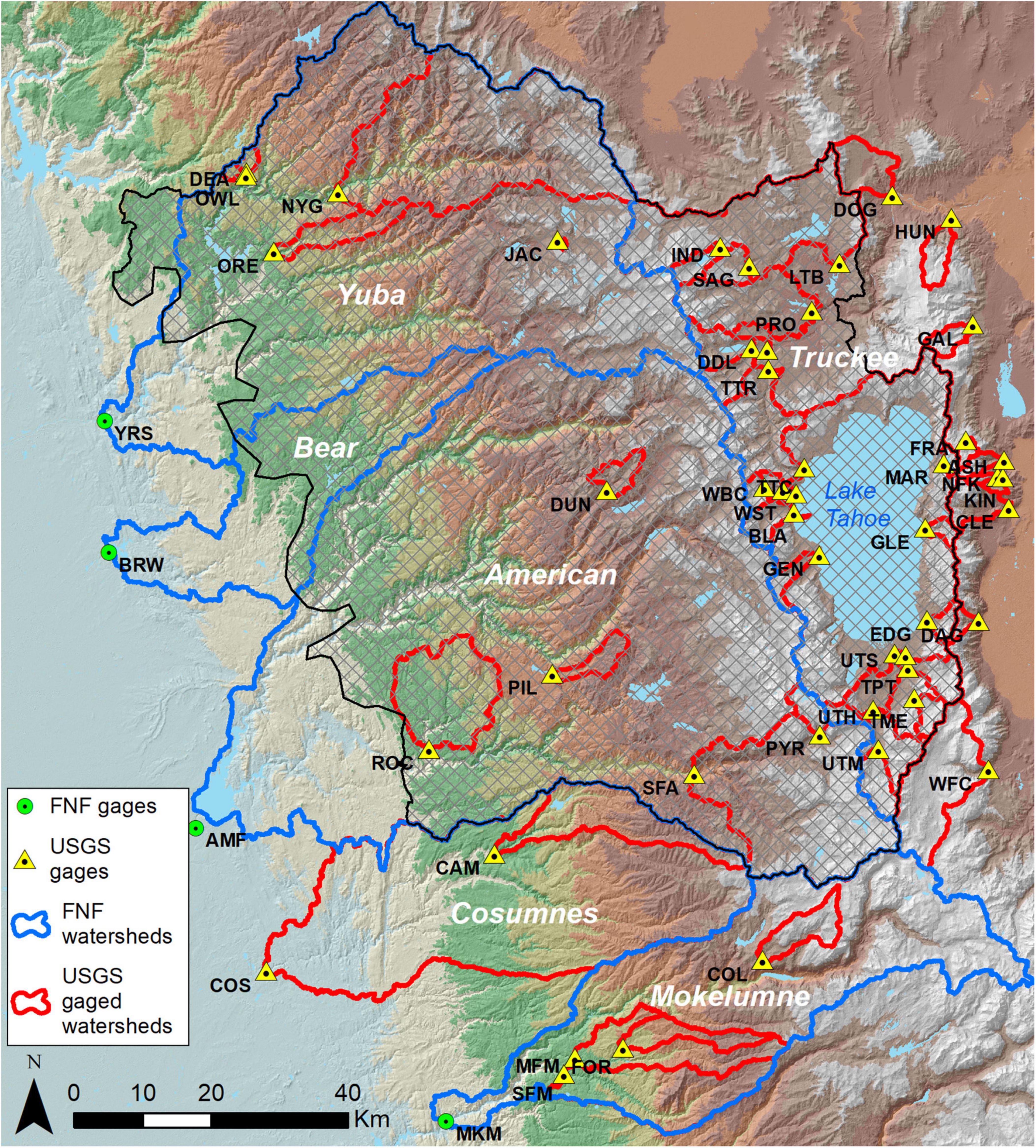
Figure 1. Study area. Watersheds outlined in blue are those for which full natural flow (FNF) data existed. The Tahoe Central Sierra Initiative project area is cross-hatched with a black outline. USGS and full natural flow gauge names, abbreviations, and locations are listed in Table 1 and Supplementary Table S1.

Study area

We evaluated the annual water balance for 48 watersheds gauged by the U.S. Geological Survey (Figure 1 and Table 1) in the upper elevations of the Yuba, Bear, American, Cosumnes, and Mokelumne basins on the west slope of the Sierra Nevada, and the upper Truckee and upper Carson basins on the east slope. We selected stream gauges with at least 10 years of record during the study period and included four larger watersheds where annual full natural flow data were available (Figure 1 and Table 2).

TABLE 1

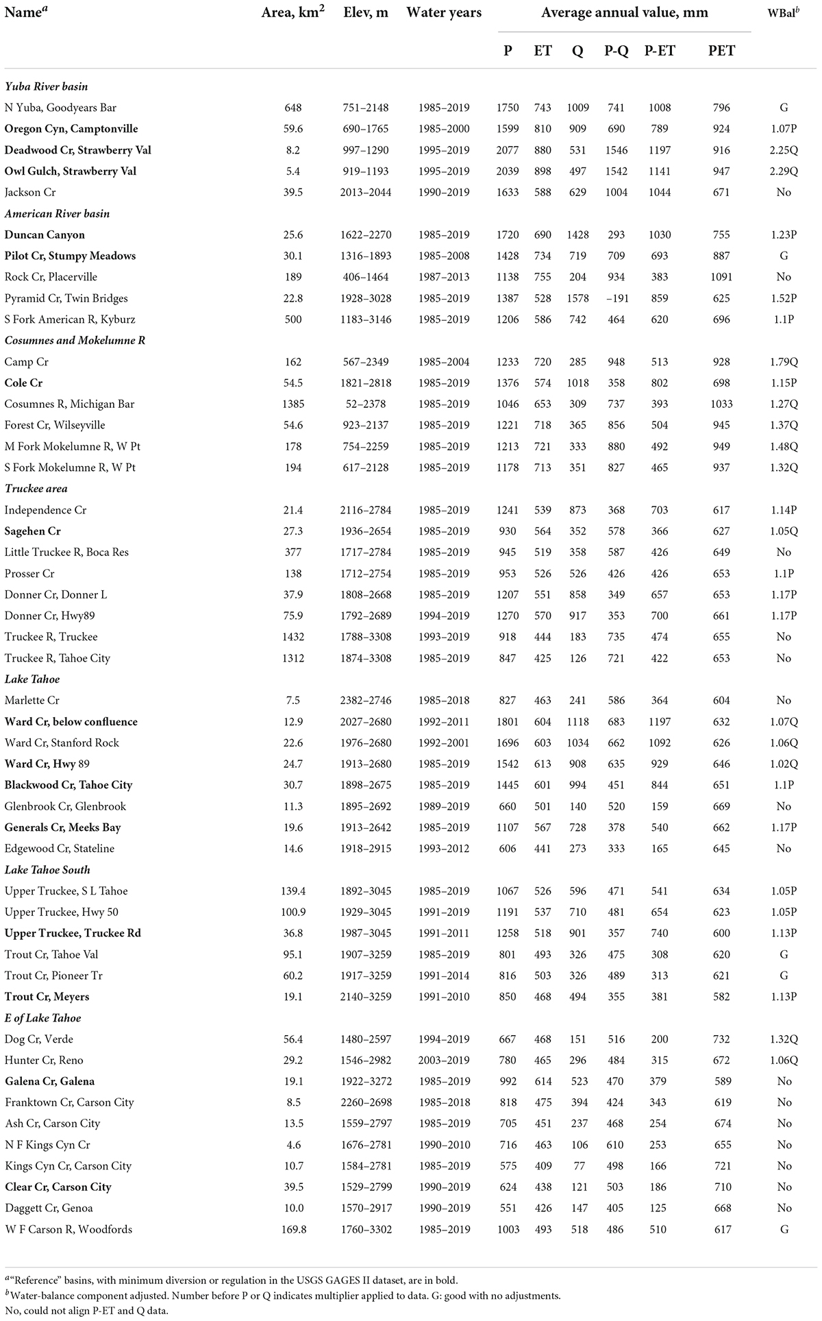
Table 1. Attributes of watersheds used in analysis.

TABLE 2

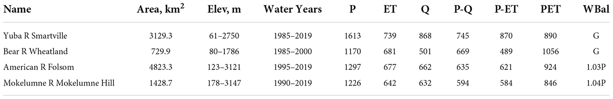
Table 2. Watersheds for which full natural flow data were available.

West of the Sierra Nevada crest, the study area is characterized by a broad slope extending approximately 80 km west to east and elevations ranging from 100 to just over 3000 m above sea level. Topographically, this mountain slope contains broad lower-relief interfluvial areas that are deeply incised by river canyons. It is heavily forested from mixed oak and conifer woodlands at lower elevations, mixed conifer at mid-elevations and red fir, Jeffrey pine and lodgepole pine forests and alpine tundra at the highest elevations (Fites-Kaufman et al., 2007). Areas east of the Sierra crest have a steeper topographic gradient compared to the west, are in the rain shadow of the range and receive approximately 50–75% less precipitation. As a result, eastside forests are less dense and contiguous compared to westside forests and dominant species at high elevations include lodgepole pine, mountain hemlock, whitebark pine, and some red fir forests. In the middle and lower elevations, the dominant species are Jeffrey pine, ponderosa pine, juniper, pinyon pine, with some white fir in moist areas (e.g., Millar, 1996; Fites-Kaufman et al., 2007; van Wagtendonk et al., 2018).

The climate is Mediterranean, characterized by cool wet winters with heavy snowpacks above 1800 m and long dry summers. The east side of the range experiences the same pattern, though drier overall due to the rain shadow formed by the range, with occasional summer monsoon-driven thunderstorms. Precipitation in the form of rain and snow occurs primarily between November and March, with average values ranging from 430 mm annually at lower elevations and east of the Sierra Nevada crest to 2200 mm at higher elevations on the west slope of the range. Mean winter (December – February) temperatures are –4.7–9.4°C, and summer temperatures (May – July) are 9.8–25.1°C at high to low elevations, respectively.

Data

For the study period 1985–2019, water-year evapotranspiration (October 1st to September 30th) was estimated using the 30-m gridded product developed by Roche et al. (2020), based on scaling measured ET at eddy covariance sites using a linear additive relationship between ET, the average of current and prior year precipitation, and NDVI from Landsat satellite data. The latter used an updated satellite data-filtering algorithm from Ma et al. (2020). ET values were capped at potential evapotranspiration (PET), which was calculated using monthly 800-m PRISM temperature data (PRISM Climate Group, 2020), methods presented in Hamon (1963), and calibrated to the maximum eddy-covariance values used in the derivation of the ET products used in this study (Fellows and Goulden, 2017). Annual precipitation, P, was derived by summing daily 800-m PRISM data and resampling to a 30-m grid aligned with the ET grids using a nearest-neighbor approach. We used annual streamflow data from USGS gauges listed in the GAGES-II dataset (United States Geological Survey [USGS], 2011) that had ten or more years of record during the study period (Table 1 and Supplementary Figure S1). In addition, we used annual full natural flow (FNF) data for the American, Mokelumne, and Yuba River watersheds¹, which accounts for diversions and changes in reservoir storage, often referred to as “unregulated flow.” Additionally, we use modeled FNF results for the Bear River watershed (California Department of Natural Resources, 2016), which is an estimate of flow in the absence of development. The latter incorporates ET estimates independent of those used here. We present FNF results separately in this study because they are derived rather than directly measured flow values. For each watershed and year of record, annual ET and P were extracted from the gridded datasets. Reported Q values were divided by the basin areas provided in the USGS dataset.

Analysis

We first classified watersheds as having diversions or not by reviewing individual gauge “Water-Year Summary” information, available watershed routing maps² (accessed May 14, 2021), and whether or not they were defined as “reference” in the GAGES-II dataset (see Table 1). Records of diversion were not available except in the case of the Deadwood Creek Powerplant near Strawberry (USGS Gage Number 11413326). Next, we examined aspects of the annual water balance (Equation 1) by first comparing plots of P vs. Q to P vs. P-ET to determine if there was alignment. In other words, we assumed that over the period-of-record ΔS was essentially zero, and mismatch was due to either bias in P-values (underestimates) or non-zero values of D. Where necessary, we then adjusted water-balance components to achieve an overall ΔS = 0, while also seeking to minimize any trend in the P-ET-Q residual. In watersheds where P vs. P-ET was lower than P vs. Q, we tried increasing P to account for underestimation, and also assessed decreasing ET to improve alignment. In watersheds where P vs. P-ET was higher than P vs. Q, we assessed proportional adjustments of Q to reflect the apparent unreported diversions, i.e., finding a multiplier (α) such that P vs. αQ was aligned with P vs. P-ET. Thus, lacking reported D values we assumed that D was a constant annual fraction of Q, so that D = Q(α-1). Note that in the figures and text, we refer to αQ as “adjusted Q.” In watersheds where the two crossed each other we attempted adjusting two water balance components, but given limited success set that aside. Finally, we determined interannual variability of apparent change in watershed subsurface storage using the annual residual of P-ET-Q, after adjusting so the mean P-ET-Q for the period of record was zero. We also used local knowledge of precipitation measurements and the existence of active rights for diversions to assess the need to adjust precipitation or account for diversions.

Results

Water balance in upper-basin headwaters

We illustrate the water-balance analysis for selected headwater watersheds across the study area that represent the range of water-balance residuals and adjustments that provided closure (Figures 2–5). Analyses for all watersheds are in Supplementary Figures S1–S7, with data summarized in Table 1.

FIGURE 2

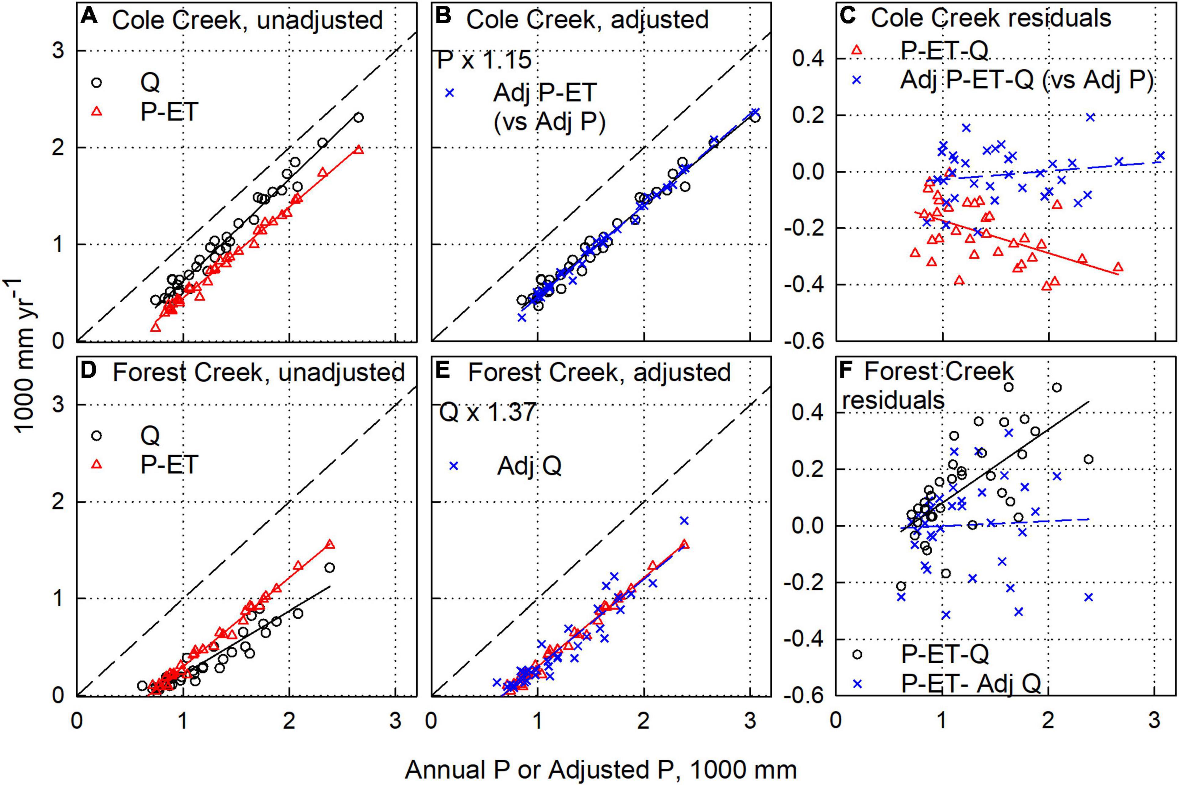
Figure 2. Illustrated process to adjust water-balance components in Cole Creek near Salt Springs Dam (A–C) and Forest Creek near Wilseyville (D–F) watersheds. (A,D) Unadjusted annual water balance components discharge (Q) and precipitation minus evapotranspiration (P-ET) versus annual precipitation (P). (B) Adjusted P-ET and Q versus adjusted P (adj P) for Cole Creek and (E) adjusted Q and P-ET versus P for Forest Creek. (C,F) Water-balance residuals (P-ET-Q) using unadjusted and adjusted components.

FIGURE 3

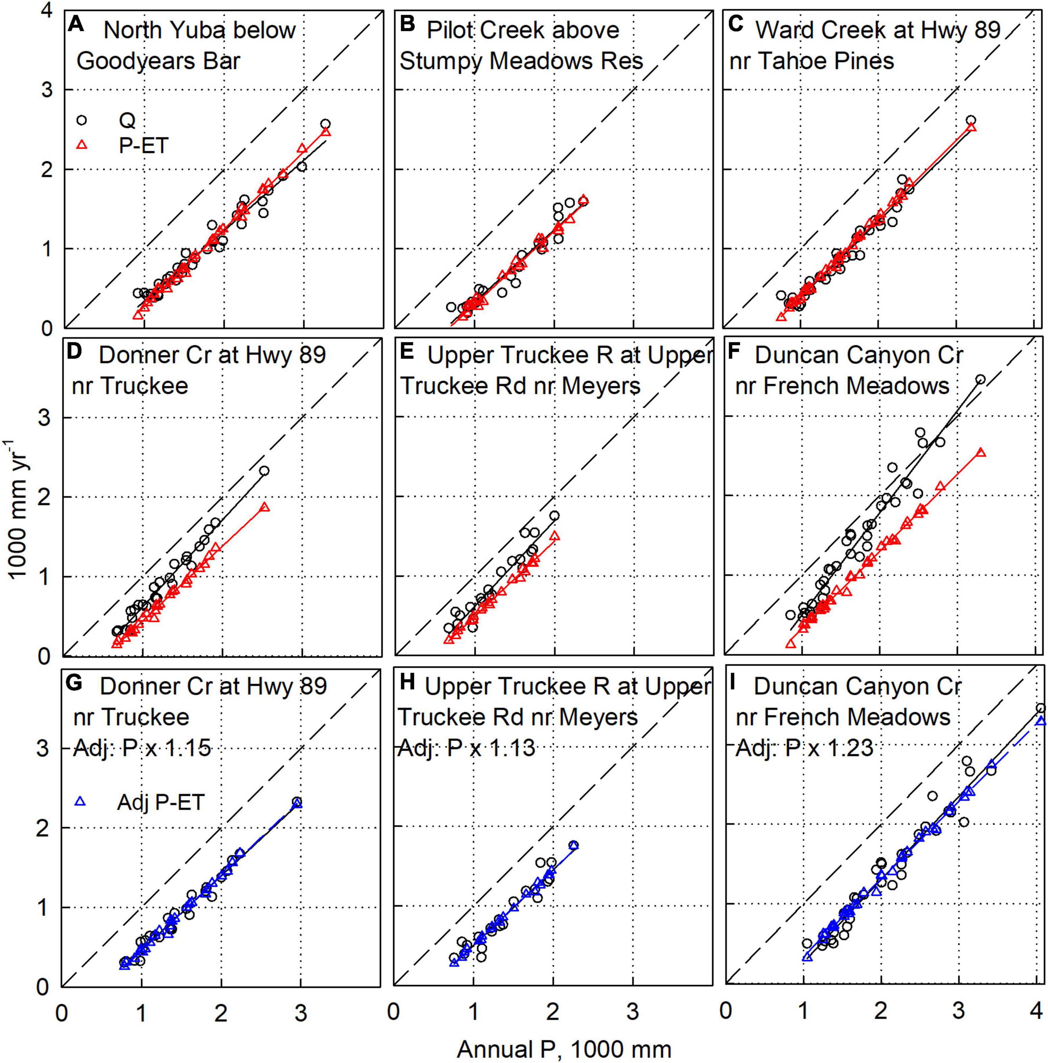
Figure 3. Water-balance analysis on representative watersheds. (A–C) Have no adjustment to P, ET, or Q values, and show average agreement between P-ET and Q within 2%. (D–F) Also have no adjustment to P, ET, or Q values, and show higher Q compared to P-ET. Thus P-values were multiplied by a constant, providing agreement between P-ET and Q (G–I). Data for additional sites is in Supplementary Figures S1–S7. The dashed diagonal is the 1:1 line.

FIGURE 4

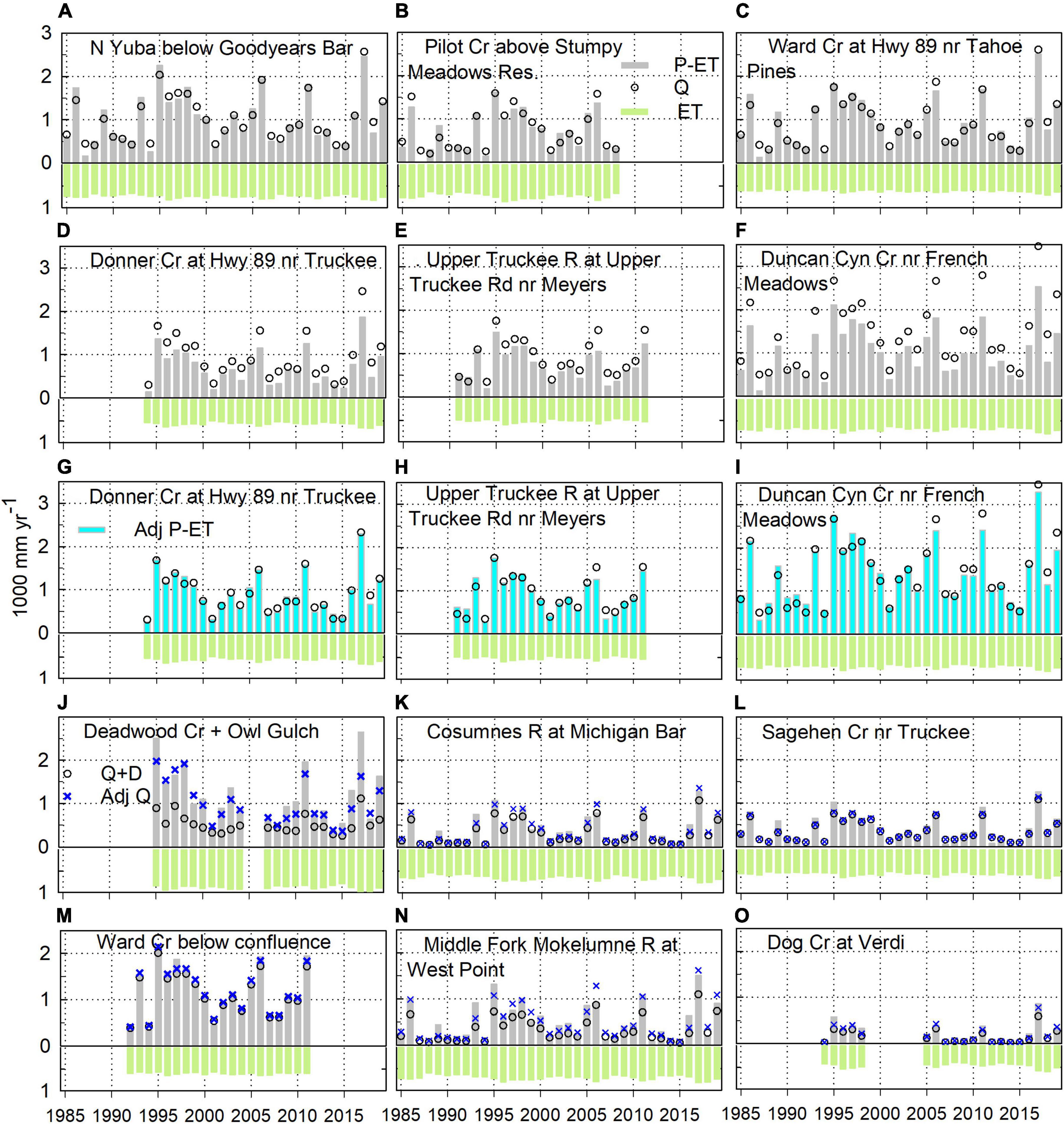
Figure 4. Water-balance time series for watersheds shown in Figure 3 (A–F) and Figure 5 (G–O). Note figure legends in (B,G,J).

FIGURE 5

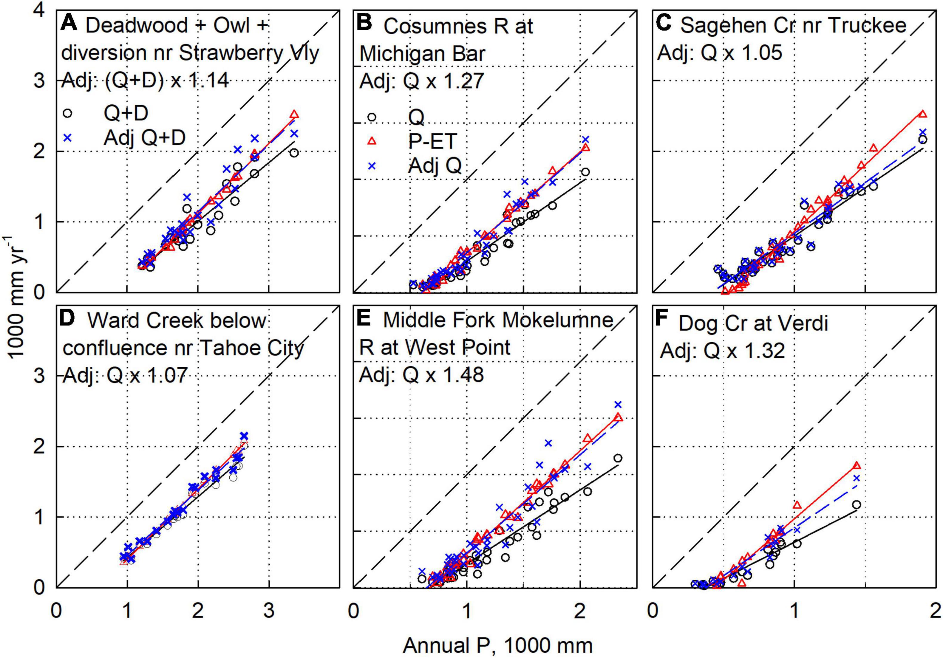
Figure 5. Water-balance analysis on representative watersheds, with adjustments to Q values. Note that each of the three columns has different scaling, with the dashed diagonal being the 1:1 line. Q values were multiplied by a constant, to improve agreement between P-ET and Q (labeled Adj Q). Note that (A) is the sum of two measured flows, with reported diversion for the combined flow added (D) in. For (A), the very wet WY 2017 was removed, owing to apparent under-measurement (see text and Figure 4J). Data for additional sites are in Supplementary Figures S1–S7.

Figure 2 illustrates the steps taken to determine what adjustments were needed, if any, to achieve balance. Cole and Forest Creeks within the Mokelumne River watershed represent typical examples with full 35-year records. Cole Creek drains higher less-vegetated and less-developed terrain, while Forest Creek drains heavily forested and more-developed areas typical of middle elevations on the west slope of the Sierra Nevada. As a first step we note that plots of Q vs. P and P-ET vs. P are not coincident, something that would be expected if the long-term residual of P-ET-Q were close to zero. Also, because annual ET varies much less than P or Q, these plots should have slopes close to one. In the case of Cole Creek, we assume that P-ET is the component likely in need of adjustment for the following reasons: (1) it is a higher elevation basin, and precipitation is likely to be underestimated because the nearest gauges are in lower and drier areas (e.g., Henn et al., 2015; Cui et al., 2022), and (2) while possible, it is highly unlikely that the stream gauge has systematically over-estimated Q for the period of record. In the case of the latter, there is no evidence of upstream regulation or flow augmentation (see references in the “Materials and methods” section). It is important to note that we adjust P-ET by proportionally increasing P 15%, which in terms of magnitude (200–400 mm yr^–1) is the more likely than a similar decrease in ET. However, we acknowledge that in some cases decreasing ET could be possible too (see “Discussion” section). These steps are depicted graphically in Figures 2A–C with additional detail in Supplementary Figure S3a.

In contrast, Forest Creek requires a multiplicative increase in Q (Figures 2D–F). While there is no evidence of flow regulation, the watershed is developed and upstream diversions associated with active water-rights permits are highly likely. The P-ET vs. P slope is close to one, consistent with low ET variability (600–800 mm yr^–1). Reducing P-ET by reducing P or increasing ET and minimizing the P-ET-Q residual (Figure 2F) would require ET to vary from approximately 600 to well over 1,200 mm yr^–1 in dry and wet years, respectively, a highly unlikely result in these highly productive forests. While some error in P and ET is possible, it is clear that the largest bias lies with Q measurements and a simple adjustment of Q results in reasonable water balance closure with respect to all three components.

For five of the 48 watersheds studied, averages of P-ET and Q for the period of record matched within 2% of P (labeled G in right-hand column of Table 1). Three are shown on Figures 3A–C. The 648 km² North Yuba below Goodyears Bar shows that average annual measured streamflow (Q) matches P-ET across the 35 years studied (Figures 3A, 4A). The match between Q and P-ET suggests that all 3 water-balance components are well constrained, which is likely the result of little upstream water use or development in this sparsely populated area (Sierra County, population = 3,200). Pilot Creek above Stumpy Meadows Reservoir also drains a rural area, with diversions for the water-rights holder occurring at the dam (Figures 3B, 4B). Ward Creek flows into Lake Tahoe, with no apparent diversions in the upper basin. The gauge shown on Figures 3C, 4C has the full 35 years of record. Two upstream gauges on Ward Creek with shorter records also show good agreement, with average Q values that are 6–7% lower than P-ET (Supplementary Figure S5a).

Fifteen additional watersheds show Q values higher than P-ET, reflecting an underestimate of P in the gridded data used for this analysis. Three of these sites are show on Figures 3D–F, and the mismatch is apparent throughout the time series (Figures 4D–F), with some reported values for Q being higher than those for P. Multiplying the annual P-values for each watershed by a constant results in a very good to excellent match between Q and P-ET. We consider the fit to be very good if the fits to the two lines are aligned with only a small difference in slopes, and excellent if they are essentially on top of each other. Increasing P by 15% in Donner Creek, 13% in the Upper Truckee River, and 23% in Duncan Canyon, aligns the fits for Q and P-ET (Figures 3G–I, 4G–I). Donner Creek is gauged at both the outlet of Donner Lake and further downstream at Highway 89, just before its confluence with the Truckee River below Lake Tahoe. Data for Q from the two gauges show excellent match with adjusted P-ET, reflecting a good water balance for the basin (Figures 3G, 4G and Supplementary Figure S4a,b). Similarly, three gauges on the Upper Truckee River above Lake Tahoe also show excellent match with adjusted P-ET (Figures 3H, 4E and Supplementary Figures S6a,b). The third example, Duncan Canyon, has a larger adjustment to P. The headwaters of Duncan Canyon have no precipitation or snow water equivalent measurement, with PRISM P-values apparently extrapolated from lower elevations. Note that P is the only component of the water balance that can plausibly be adjusted at these sites. Adjusting ET would not improve the alignment of P-ET with Q. While adjusting Q downward could also improve the alignment, it was assumed that there was less uncertainty in Q than in P for these well-maintained stream gauges; and adjusting Q could align the long-term means, but not the annual values of the P-ET and Q on Figures 3, 4.

For an additional 13 sites, adjusting Q values provided some degree of alignment between annual P-ET and Q values. Deadwood Creek and Owl Gulch watersheds (combined area 13.6 km²) have hydropower diversions, as evidenced by a lower slope of Q compared to P-ET (Supplementary Figure S1b). Adding in reported annual D values more closely aligns the two data sets, with D being about 2/3 of D + Q in wet years, and as low as 10% of D + Q in dry years (Figure 5A). However, the remaining mismatch suggest a missing increment averaging at least 14% higher than the reported D + Q values, with the mismatch being mainly in wetter years (Figure 4J). The plot of Q versus P for Cosumnes River at Michigan Bar also has a lower slope than does P-ET (Figure 5B). There are likely a number of upstream diversions, and multiplying annual Q values by 1.27 aligns the P-ET and Q data (Figures 4K, 5B).

Values of Q for the eastern-Sierra Sagehen Creek watershed illustrate a different and less consistent pattern. In drier years, Q values are generally higher than P-ET, and exhibit considerable scatter (Figure 5C). Though the slope of the Q vs. P line is similar to that for Forest Creek (Figure 2D), multiplying Q values for Sagehen by a constant pushes the fitted line for Q higher than that for P-ET, with only small changes in slope. A multiplier of 1.05 is shown on Figure 5C, but even with an increase in the multiplier to 1.2, to increase the slope of Q versus P, significant offsets remain. This is especially apparent in wet years (Figure 4L). However, the lower values of Q and P-ET also do not line up, with Q much greater than P-ET in drier years. Given that the Sagehen stream gauge is just below a meadow, with limited bedrock control, it is plausible that outflow from the basin is much higher than measured. Decreasing ET could align these lower values, but the slope of Q vs. P (0.68 in Figure 5C) would still be much lower than 1.0. Increasing Q by 40% combined with decreasing ET by 20–25% more closely aligns the Q and P-ET data. However, reducing ET would make values lower than the surrounding area. These findings, plus the large scatter in the Q values for Sagehen, suggest that the streamflow data in this watershed may not provide a good water-balance control.

Figures 4M, 5D show the adjustment to the upstream Ward Creek Q values noted above, and the alignment of the adjusted Q with P-ET. A much larger adjustment was made for the Middle Fork Mokelumne River, with good results in alignment (Figures 4N, 5E). Adjusting Q for the east-side Dog Creek watershed aligns lower to mid Q and P-ET values, with the higher Q values still lower than P-ET (Figures 4O, 5F).

Interannual variability in water balance and ΔS

Once diversions or underestimates of streamflow or precipitation are adjusted, the interannual variability in water-balance residuals (P-Q-ET-D) generally lie within + 300 mm yr^–1, with a very weak trend with respect to current-year precipitation (Figure 6A). The residual does, however, generally decrease with respect to increasing previous-year precipitation (Figure 6B). That is, measured Q tends to exceed P-ET in drier years that follow wet years and vise-versa. There are certain obvious exceptions such as Oregon Canyon after 1996, where Q consistently exceeds P-ET (Supplementary Figure S1a) suggesting a change in conditions. The green ET bars in all panels of Figure 4 show that annual evapotranspiration varies little relative to the water balance of P-Q-D. In the dry year 1987, ET exceeds P across some basins, resulting in near-zero runoff. The cumulative water-balance residual for these same watersheds showed a small change or no net change over time (Supplementary Figures S8a,b) and was within +450 mm yr^–1 for two of the full-natural-flow basins (Supplementary Figure S8c). It is notable that the cumulative residual is progressively negative for the Mokelumne and American full-natural-flow watersheds (Supplementary Figure S8c).

FIGURE 6

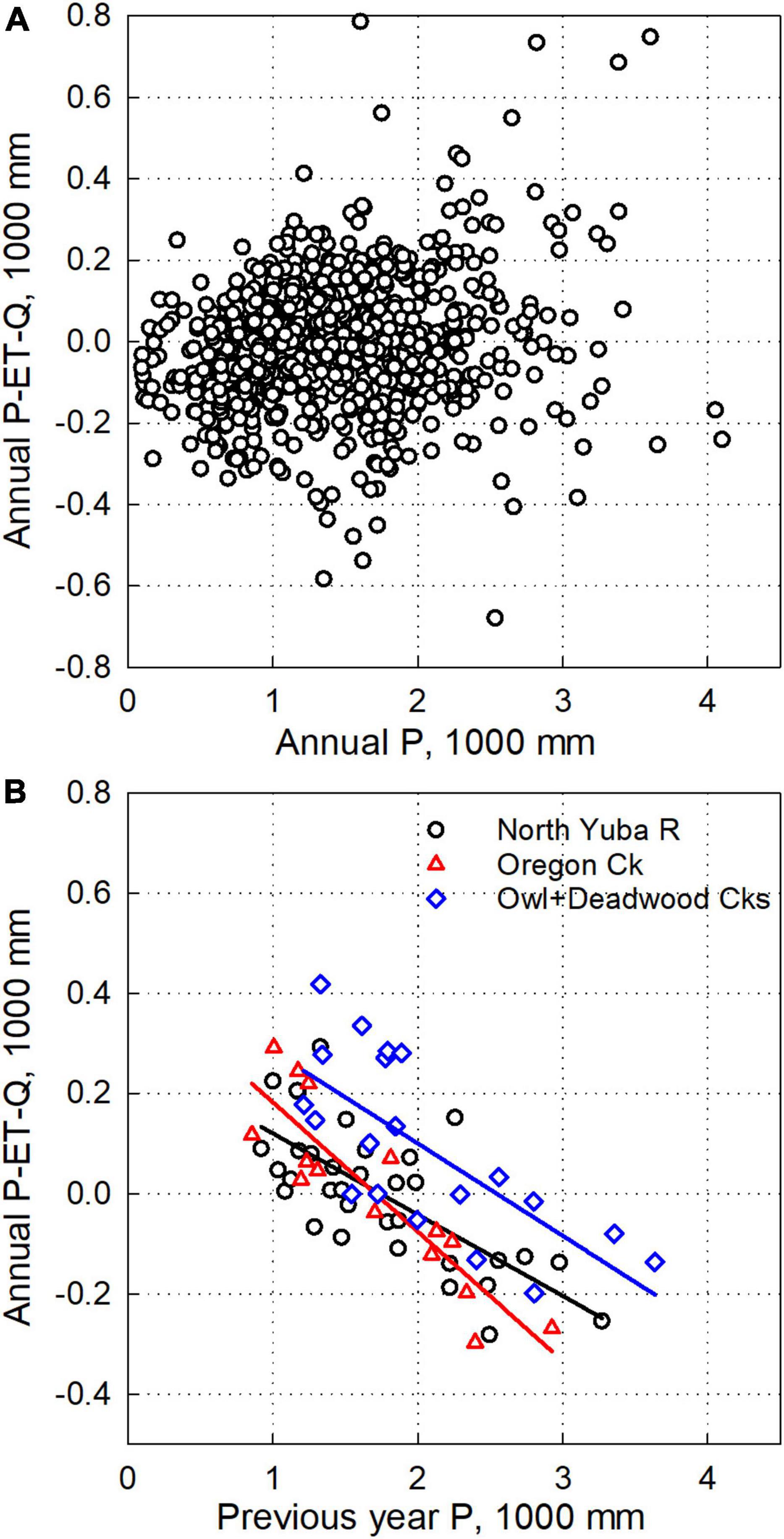
Figure 6. (A) Water-balance residual for 24 separate (not overlapping) USGS GAGES-II watersheds: 4 requiring no adjustment, 15 where P was adjusted, and 5 watersheds with good water balance after Q adjustment (Forest Creek, Middle and South Forks Mokelumne, Ward Creek below Confluence and at Stanford Rock). (B) Water balance residual versus prior year precipitation for Yuba River watersheds. Regression equations are: ResidualNorthYuba = –0.1621 × PriorYearP + 282, R² = 0.51 (p < 0.0001), ResidualOregonCk = –0.2581 × PriorYearP + 440, R² = 0.79 (p < 0.0001), ResidualOwl + Deadwood = –0.1842*PriorYearP + 468, R² = 0.51 (p = 0.0004).

Water balance across larger basins

FNF versus P for larger watersheds (730–4823 km²) shows good consistency across all years (Figure 7). The Yuba River has the highest P and thus greatest FNF, followed by the American and Mokelumne. These higher values for the Yuba largely reflect its higher latitude. The lower-elevation Bear R basin has lower P and FNF, and also shows a greater dependence of P-FNF on P. That is, ET apparently shows a greater response to P in this lower-elevation basin. Alternatively, the slope of FNF vs. P could reflect additional discharge not accounted for in the FNF.

FIGURE 7

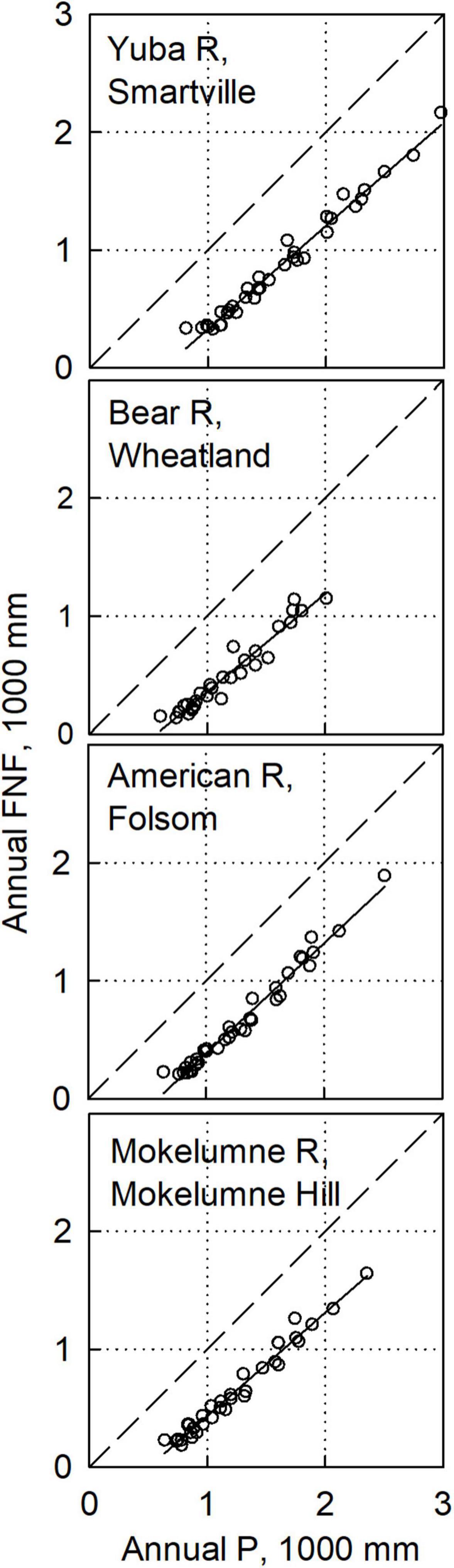
Figure 7. Water-balance analysis for Full Natural Flow basins. The dashed diagonal is the 1:1 line.

Discussion

Overall water balance

Of the 48 gauged watersheds plus the 4 full-natural-flow gauges evaluated, 31 provided a very good water balance using three independent datasets for P, ET, and Q. These included data from 5 gauges plus 2 full-natural flow watersheds where P adjustment was less than 2%. An additional 17 provided an equally good water balance with generally small adjustments to P. The median adjustment was 13%, with only 2 over 20% (Duncan Canyon 23% and Pyramid Creek 52%). These latter two large adjustments we generally attribute to the sparse precipitation measurements in those higher-elevation parts of the American River basin, though ET may be over-estimated in the sparsely vegetated Pyramid watershed (see below). After adjustment, four of the five headwater gauges in the American basin, two of the five in the Yuba, and four of the eight in the Truckee area provided very good water balance. All six of the gauges in the Lake Tahoe South area, on the Upper Truckee River and Trout Creek, had very good water balance with either small adjustments to P or no adjustments.

Of the 13 basins to which we made adjustments to Q, eight provided very good water balances. Three were in the Lake Tahoe basin, on Ward Creek, with adjustments of 2–7%. The other 5 were in the Cosumnes and Mokelumne watersheds, with adjustments of 27–79%. Thus, after adjustment all six of the gauges in the Cosumnes and Mokelumne basins had very good water balances.

The remaining five gauges to which we made adjustments to Q provided water balances that we consider usable for further analysis, but with greater uncertainty. These include Owl Gulch and Deadwood Creeks in the Yuba, Sagehen in the Truckee area, plus Dog and Hunter Creeks east of Lake Tahoe. The remaining 15 basins had poor water balances. It is our assessment that for all of these watersheds, the main uncertainty was in Q and/or D. Examples include the Q versus P plots for Rock and Marlette Creeks, which exhibit large scatter, particularly in the adjusted Q values (Supplementary Figures S2b, S5c).

Annual and study-period-average water-balance values also show a consistent pattern using the Budyko framework (Figure 8). Figures 8A–C depict contrasts between energy and water-limited areas on the west side of the Sierra Nevada crest (North Yuba and Cosumnes River watersheds), smaller watersheds west and east of the crest (Duncan Canyon and Dog Creek), and watersheds east of the crest that differ in mean elevation (Upper Truckee and Trout Creek, higher and lower elevation, respectively). These figures illustrate that annual values in more-arid locations exhibit greater variability, with slopes less than one. The Cosumnes River and Dog Creek watersheds have similar mean aridity, though the Cosumnes is driven by higher mean annual temperature due to its lower elevation (944 versus 1,932 m) and Dog Creek is driven by lower mean annual precipitation (667 versus 1,046 mm yr^–1). Annual values for the adjacent Upper Truckee River and Trout Creek areas (Figure 8C) align for the higher (cooler) and wetter Upper Truckee to the lower (warmer) and drier Trout Creek watershed. Most study watersheds are energy limited, with ET comprising 50% or less of the annual precipitation input. More-water-limited sites tended to be low-elevation watersheds and sites substantially east of the Sierra Nevada crest in the rain shadow cast by the range. This consistency is evident across all study locations, as shown in Figure 8D, where the exponential best fit is the same for westside, eastside, and all site regressions. The exponential fit (b = 2.59) is comparable to mean values in Zhang et al. (2004), though lower than that reported for forested areas in that study reflecting the mix of forested and unforested areas in this study. Hence, the ET values reported here produce aridity relations that are robust across a large elevation and precipitation range and are consistent with other research.

FIGURE 8

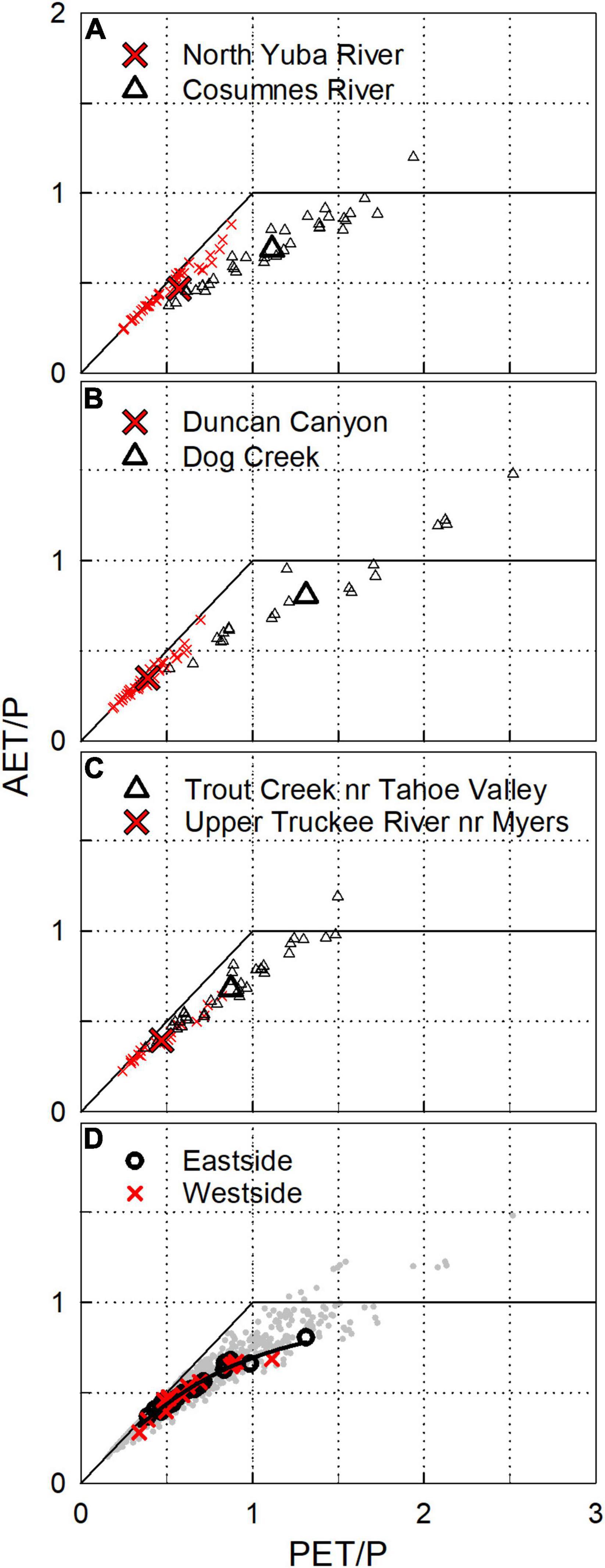
Figure 8. Budyko diagrams, precipitation-normalized potential evapotranspiration (PET/P) versus precipitation-normalized actual evapotranspiration (AET/P). (A–C) Mean and annual values as large and small symbols, respectively. (D) All mean (bold symbols) and annual values (gray dots) for gaged watersheds in this study. The best fit line for mean watershed values in (D) is AET/P = 1 + PET/P – (1 + (PET/P)^b)^(1/b) where b = 2.5928 (R-squared = 0.97).

Assessing water-balance components

Overall, ET measurements were robust across the range of elevations and mountain-vegetation types represented in this study. That is, the good basin-scale water balances previously observed in larger-basin water-balance assessments in the Sierra Nevada (Roche et al., 2020; Rungee et al., 2021) are also apparent in the smaller headwater basins across mid to higher elevations that were the subject of the current analysis. After accounting for apparent diversions (adjusted Q) and underestimated precipitation (adjusted P) we found very good to excellent water balances across 33 of the 48 headwater watersheds. While ET reductions of 5–10% may be appropriate in some cases, uncertainty in annual Q and P is apparently larger, and thus adjustments to those components are more appropriate. We estimate that while uncertainty in ET from a given flux tower used to develop the gridded ET data could be as much as 20%, the uncertainty should be random from tower to tower, and to a lesser extent year to year, so the overall uncertainty should be less for the full dataset (Rungee et al., 2021). NDVI values, resolved in our study at 30-m from Landsat, are correlated with ET in the Sierra Nevada (Goulden et al., 2012; Goulden and Bales, 2014). In the current analysis, we use ET estimates that are based on two variables, P as well as NDVI (Roche et al., 2020). Our P-values, from PRISM, are an 800-m gridded product, and fail to capture the multi-scale variability in higher-elevation precipitation – snow accumulation – observed by Lidar (Zheng et al., 2016), snow pillows (Kirchner et al., 2014), or snow courses (Rice and Bales, 2010). We previously assessed that the total uncertainty in precipitation may be near or less than the reported west-wide potential annual interpolation error of ±98 mm for PRISM in rain-dominated areas with more data, and upwards of 50% or more in snow-dominated, open areas (Rungee et al., 2021).

It is important to discuss circumstances where ET may be over-estimated. The ET product was developed using flux-tower data in forested areas of the Sierra Nevada as well as lower-elevation shrub and grasslands. Application in high-elevation sparsely vegetated areas likely over estimates ET due to an over-dependence on current- and prior-year precipitation. Comparison with an optimized version of the regression used in this study (see “Materials and methods” section) illustrates that reducing the influence of P substantially affects the value of ET in watersheds such as Pyramid Creek (Figure 9). The optimized ET calculation adjusts the coefficients in Equation S2 from Roche et al. (2020) to 0.8 and 0.2 for NDVI and PP components, respectively. This version produces robust results in larger watersheds (Supplementary Figure S9) and will serve as an important starting point for future work.

FIGURE 9

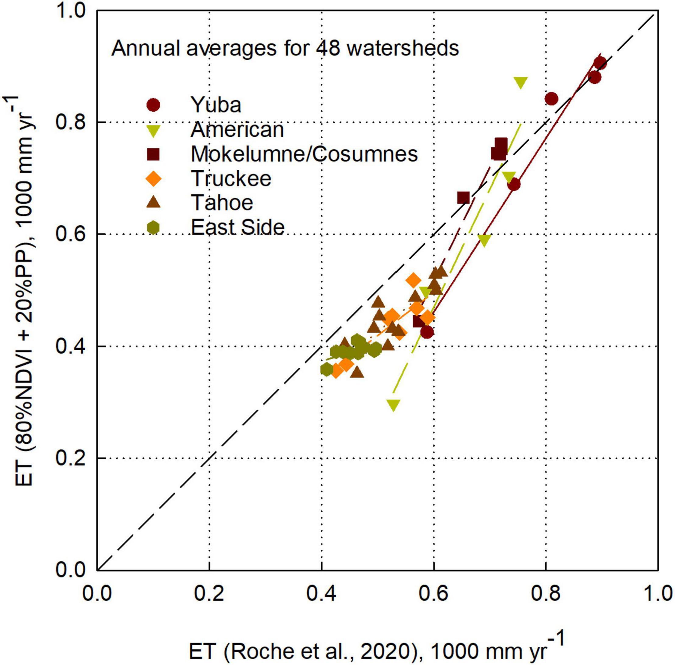
Figure 9. ET comparison between Roche et al. (2020) regression and 0.8NDVI + 0.2PP weighting regression. The two approaches compare well for well-vegetated west-slope watersheds (Yuba, American, and Mokelumne/Cosumnes). The Roche et al. (2020) regression produces higher ET values for east-slope and more sparsely-vegetated watersheds (Truckee, Tahoe, East Side, and the Pyramid watershed in the American – lower most inverted triangle).

In watersheds requiring an adjusted water balance and where diversions were small, increasing P generally improved water-balance results, with no adjustments to Q. The range of P adjustments (2–50%) is consistent with undercatch in high-elevation and latitude mixed-phase precipitation measurements of approximately 20–70% (e.g., Yang et al., 1998; Fassnacht, 2004), plus propagation of this uncertainty through interpolation and extrapolation to develop gridded products, particularly where point data are limited. Yet for this study, the good alignment of P-ET and Q after adjustment of P and given that most adjustments to P were under 15%, indicate sufficient quality in the spatial estimates of precipitation across the broad elevation and geographic range of this study for evaluating the ET product and overall water balance.

Watersheds where higher adjustments to P were needed were areas with no nearby rain-snow precipitation gauges or snow pillows, and uncertainty in these measurements are consistent with those reported elsewhere (e.g., Henn et al., 2015; Cui et al., 2022) and obvious because discharge often exceeded precipitation. Precipitation estimates east of the Sierra Crest appeared quite robust, despite being an area of strong gradients, which is likely the result of more high-quality mixed-phase precipitation gauges placed systematically throughout the Truckee River watershed and Tahoe basin.

Discharge was adjusted in many basins where records indicated substantial diversions. In some cases, a simple multiplier was sufficient, though in reality diversions may be limited by capacity at high flows and other factors such as minimum in-stream flow requirements. Adjustment to discharge were increases of 30–100%, well beyond the expected error in flow measurements. Stream-gauge records in the GAGES-II dataset exhibit low daily flow estimates when stage measurements were not available (mean = 5.3%). Most gauge records have a “fair” rating, indicating an approximate error of 15%. Sauer and Meyer (1992) suggest a poor rating to be associated with an error of approximately 20%. Locations where adjustments were not possible were generally areas where the stream gauge did not fully capture flows or the pattern of diversions did not lend itself to a simple multiplicative correction (Supplementary Figure S10).

Data on diversions above measured stream gauges was quite limited. For the one site we found in the state’s water-rights data base, the combined Deadwood and Owl in the Yuba, adding in the diversion did not give Q + D values that matched P-ET. However, this data set points to two issues relevant to sites without reported D values. First, it must be recognized that publicly accessible, accurate diversion data for most sites in the Sierra Nevada are not available. Second, it is recognized that in practice diversions are not simply a multiplier, but may have a non-linear dependence on annual P and Q (e.g., Supplementary Figure S10). Thus, while some of our adjustments to Q reflect diversions, there may also be subsurface flow leaving a basin, or uncertainty in measured flow or FNF (e.g., Supplementary Figure S8c).

Annual water-balance residuals indicate potential interannual changes in subsurface storage (ΔS) in the range of + 300 mm, which given potential errors among components may be regarded as a basepoint for investigating forest resilience to drought. In dry years, a decrease in subsurface storage of 300 mm is approximately 40–50% of annual evapotranspiration and generally more water than would be expected in the top 1 m of soil (Bales et al., 2018). While some of this difference may be due to errors in the measurement of Q and P, the relation between prior-year precipitation and change in storage (Figure 6B) suggests that carryover surplus or deficit precipitation from the previous year does influence runoff in the current year, consistent with findings elsewhere (Godsey et al., 2013; Klos et al., 2018; Roche et al., 2018). Using data from the Yuba River watersheds in Figure 6B, one may expect Q to be augmented in a dry year following a wet year by approximately 100 mm for every 500 mm above average precipitation in the prior year. Similarly, following a dry year, discharge may be reduced by 100 mm for every 500 mm precipitation is reduced.

Limitations

In order to examine water balance across a broad study domain, our study sought to use available high-quality streamflow measurements and spatial estimates of precipitation using 800-m resolution PRISM data and evapotranspiration estimates. As discussed above, each data source contains bias due to available station locations (precipitation), unknown or unmeasured diversion (streamflow), or groundwater losses due to pumping or flow around stream gauges. We used watershed areas provided by the USGS GAGES II dataset, which could be another source of error. The ET estimate is based on a combination of vegetation greenness (annual averaged NDVI) and the mean of the current- and previous-year precipitation. While this method has been shown to produce robust results (Supplementary Figure S9; Rungee et al., 2021), the dependence on precipitation mutes the impacts of changes in vegetation due to fire, drought mortality, or increasing forest density over time. This makes it difficult to assess trend at the time scale of 35 years (1985–2019). Additionally, this method was developed for vegetated areas and applying it to sparsely vegetated alpine regions may require refinements that were beyond the scope of this study, as discussed in reference to Figure 9. Adjusting P upwards by 15% increases ET by 5–8%, a potential complication not explicitly addressed in this study due to the high spatial variability in P. Nevertheless, when capping ET estimates to PET, the model produces consistent results. Finally, we use a standard method for calculating PET (Hamon, 1963). Future efforts may benefit from a more thorough consideration of PET as it affects ET estimates (capping) or subsurface-water-use estimates.

It should be noted that our adjustments to P and Q were in part indexed to achieving ΔS = 0 averaged over the study period. That is, we assumed no net change in storage over the periods of record for each stream gauge. Across our data, annual ΔS estimated as P-Q-ET increased with P for some sites, reflecting uncertainty in the component data, but did not show trends over time (Supplementary Figure S8). An increase or decrease in the cumulative P-Q-ET residual over time, exhibited in the American and Mokelumne full-natural-flow basins, could be due to groundwater exchange (ΔS), unaccounted for deep subsurface flows, or systematic or random errors in measurements.

Improving water balances in the study area should focus on areas where point measurements are lacking, and quality mixed-phase precipitation measurements at higher elevations in mountainous terrain. Public availability of diversion data is also an issue, and will depend on both better measurements and reporting.

Conclusion

High-quality spatial evapotranspiration (ET) estimates, together with best-available gridded precipitation (P) data and measured stream discharge (Q) resulted in good water-balance closure across a range of central Sierra Nevada watershed sizes, elevations, and aridities. Uncertainties in water balance over the period of record for watersheds defined by stream gauges with no apparent diversion ranged from 0 to 52% of watershed-average precipitation. The median water-balance uncertainty across these watersheds was 10% of precipitation. After adjusting precipitation or discharge to align annual P-ET and Q values for each watershed, average residuals in overall water balance averaged zero for over 70% of the watersheds studied. For about 30% of the watersheds studied, issues with discharge estimates and non-linear diversions made simple adjustments not possible. ET estimates appear to be accurate to within 5–10% except in alpine areas as noted in the discussion, well below potential errors in discharge measurements (up to 20% without diversions) and mapped annual precipitation (up to 52%). Closing the water balance on 33 of 48 watersheds (excluding the 4 FNF records) permitted estimates of potential changes in annual subsurface water storage of + 300 mm. Overall, results show that using accurate spatial ET estimates permit identification of potential bias in precipitation or discharge estimates, as well as providing a powerful tool for tracking interannual water balance variation in mountain watersheds.

Data availability statement

Publicly available datasets were analyzed in this study. This data can be found here: https://prism.oregonstate.edu/, https://waterdata.usgs.gov/nwis/sw.

Author contributions

JR: conceptualization, methodology, investigation, visualization, writing – original draft, and writing – review and editing. KW: investigation, visualization, and writing – review and editing. QM: investigation. RB: supervision, funding acquisition, conceptualization, resources, investigation, writing – original draft, and writing – review and editing. All authors contributed to the article and approved the submitted version.

Funding

Primary support for this research was provided by The Nature Conservancy, as part of the Tahoe-Central Sierra Initiative. Supplemental support was provided by the U.S. National Science Foundation through the Southern Sierra Critical Zone Observatory (EAR-1331939), a USDA Small Business Innovation Research grant to Blue Forest Conservation, and from the California Strategic Growth Council through the Innovation Center for Ecosystem Climate Solutions.

Conflict of interest

The authors declare that the research was conducted in the absence of any commercial or financial relationships that could be construed as a potential conflict of interest.

The reviewer GD declared a shared affiliation with one of the authors RB to the handling editor at the time of review.

Publisher’s note

All claims expressed in this article are solely those of the authors and do not necessarily represent those of their affiliated organizations, or those of the publisher, the editors and the reviewers. Any product that may be evaluated in this article, or claim that may be made by its manufacturer, is not guaranteed or endorsed by the publisher.

Supplementary material

The Supplementary Material for this article can be found online at: https://www.frontiersin.org/articles/10.3389/ffgc.2022.861711/full#supplementary-material

Footnotes

1. ^ https://cdec.water.ca.gov/
2. ^ https://ca.water.usgs.gov/data/waterdata/schematics2007.html

References

Avanzi, F., Rungee, J., Maurer, T., Bales, R., Ma, Q., Glaser, S., et al. (2020). Climate elasticity of evapotranspiration shifts the water balance of Mediterranean climates during multi-year droughts. Hydrol. Earth Syst. Sci. 24, 4317–4337.

Google Scholar

Bales, R. C., and Dietrich, W. E. (2020). Linking critical zone water storage and ecosystems. Eos 101. doi: 10.1029/2020EO150459

CrossRef Full Text | Google Scholar

Bales, R. C., Goulden, M. L., Hunsaker, C. T., Conklin, M. H., Hartsough, P. C., O’Geen, A. T., et al. (2018). Mechanisms controlling the impact of multi-year drought on mountain hydrology. Sci. Rep. 8:690. doi: 10.1038/s41598-017-19007-0

PubMed Abstract | CrossRef Full Text | Google Scholar

Bales, R. C., Hopmans, J. W., O’Geen, A. T., Meadows, M., Hartsough, P. C., Kirchner, P., et al. (2011). Soil moisture response to snowmelt and rainfall in a Sierra Nevada mixed-conifer forest. Vadose Zone J. 10, 786–799. doi: 10.2136/vzj2011.0001

CrossRef Full Text | Google Scholar

California Department of Natural Resources (2016). Draft. Estimates of Natural and Unimpaired Flows for the Central Valley of California: Water Years 1922-2014. Available Online at: https://cawaterlibrary.net/wp-content/uploads/2018/03/Estimates-of-Natural-and-Unimpaired-Flows-for-the-Central-Valley-of-California-1922-2014.pdf (accessed January 24, 2021).

Google Scholar

Cui, G., Ma, Q., and Bales, R. (2022). Assessing multi-year-drought vulnerability in dense Mediterranean-climate forests using water-balance-based indicators. J. Hydrol. 606:127431. doi: 10.1016/j.jhydrol.2022.127431

CrossRef Full Text | Google Scholar

Fassnacht, S. R. (2004). Estimating Alter-shielded gauge snowfall undercatch, snowpack sublimation, and blowing snow transport at six sites in the coterminous USA. Hydrol. Process. 18, 3481–3492. doi: 10.1002/hyp.5806

CrossRef Full Text | Google Scholar

Fellows, A. W., and Goulden, M. L. (2017). Mapping and understanding dry season soil water drawdown by California montane vegetation. Ecohydrology 10:e1772. doi: 10.1002/eco.1772

CrossRef Full Text | Google Scholar

Fites-Kaufman, J. A., Rundel, P., Stephenson, N., and Weixelman, D. A. (2007). “Montane and subalpine vegetation of the Sierra Nevada and Cascade ranges,” in Terrestrial Vegetation of California, eds M. G. Barbour, T. Keeler-Wolf, and A. A. Schoenherr (Berkeley: University of California Press), 456–501.

Google Scholar

Godsey, S. E., Kirchner, J. W., and Tague, C. L. (2013). Effects of changes in winter snowpacks on summer low flows: case studies in the Sierra Nevada, California, USA. Hydrol. Process. 28, 5048–5064. doi: 10.1002/hyp.9943

CrossRef Full Text | Google Scholar

Goulden, M. L., and Bales, R. C. (2019). California forest die-off linked to multi-year deep soil drying in 2012–2015 drought. Nat. Geosci. 12, 632–637. doi: 10.1038/s41561-019-0388-5

CrossRef Full Text | Google Scholar

Goulden, M. L., Anderson, R. G., Bales, R. C., Kelly, A. E., Meadows, M., and Winston, G. C. (2012). Evapotranspiration along an elevation gradient in California’s Sierra Nevada. J. Geophys. Res. Biogeosci. 117:G03028. doi: 10.1029/2012JG002027

CrossRef Full Text | Google Scholar

Goulden, M. L. and Bales, R. C. (2014). Mountain runoff vulnerability to increased evapotranspiration with vegetation expansion. Proc. Natl. Acad. Sci. U.S.A. 111, 14071–14075. doi: 10.1073/pnas.1319316111

PubMed Abstract | CrossRef Full Text | Google Scholar

Hamon, W. R. (1963). Estimating potential evapotranspiration. Trans. Am. Soc. Civil Eng. 128, 324–338. doi: 10.1061/TACEAT.0008673

PubMed Abstract | CrossRef Full Text | Google Scholar

Henn, B., Clark, M. P., Kavetski, D., and Lundquist, J. D. (2015). Estimating mountain basin-mean precipitation from streamflow using Bayesian inference. Water Resour. Res. 51, 8012–8033. doi: 10.1002/2014WR016736

CrossRef Full Text | Google Scholar

Kirchner, P. B., Bales, R. C., Molotch, N. P., Flanagan, J., and Guo, Q. (2014). LiDAR Measurement of Seasonal Snow Accumulation along an Elevation Gradient in the Southern Sierra Nevada, California. Hydrol. Earth Syst. Sci. 18, 4261–4275.

Google Scholar

Klos, P. Z., Goulden, M. L., Riebe, C. S., Tague, C. L., O’Geen, A. T., Flinchum, B. A., et al. (2018). Subsurface plant-accessible water in mountain ecosystems with a Mediterranean climate. Wiley Interdiscip. Rev. 5:e1277. doi: 10.1002/wat2.1277

CrossRef Full Text | Google Scholar

Lundquist, J., Hughes, M., Gutmann, E., and Kapnick, S. (2019). Our skill in modeling mountain rain and snow is bypassing the skill of our observational networks. Bull. Am. Meteorol. Soc. 100, 2473–2490. doi: 10.1175/BAMS-D-19-0001.1

CrossRef Full Text | Google Scholar

Ma, Q., Bales, R. C., Rungee, J., Conklin, M. H., Collins, B. M., and Goulden, M. L. (2020). Wildfire controls on evapotranspiration in California’s Sierra Nevada. J. Hydrol. 590:125364. doi: 10.1016/j.jhydrol.2020.125364

CrossRef Full Text | Google Scholar

Millar, C. I. (1996). Sierra Nevada Ecosystem Project. Sierra Nevada Ecosystem Project, Final Report to Congress, Vol. I, Assessment Summaries and Management Strategies, Centers for water and Wildland Resources. Report No 36. Davis: University of California.

Google Scholar

O’Geen, A., Safeeq, M., Wagenbrenner, J., Stacy, E., Hartsough, P., Devine, S., et al. (2018). Southern sierra critical zone observatory and kings river experimental watersheds: a synthesis of measurements, new insights, and future directions. Vadose Zone J. 17, 1–18. doi: 10.2136/vzj2018.04.0081

CrossRef Full Text | Google Scholar

PRISM Climate Group (2020). Oregon State University. Available Online at: http://prism.oregonstate.edu, created (access June 30, 2020).

Google Scholar

Rice, R., and Bales, R. C. (2010). Embedded-sensor network design for snow cover measurements around snow pillow and snow course sites in the Sierra Nevada of California. Water Resour. Res. 46:W03537. doi: 10.1029/2008WR007318

CrossRef Full Text | Google Scholar

Roche, J. W., Goulden, M. L., and Bales, R. C. (2018). Estimating evapotranspiration change due to forest treatment and fire at the basin scale in the Sierra Nevada, California. Ecohydrology 11:e1978. doi: 10.1002/eco.1978

CrossRef Full Text | Google Scholar

Roche, J. W., Ma, Q., Rungee, J., and Bales, R. C. (2020). Evapotranspiration mapping for forest management in California’s Sierra Nevada. Front. For. Glob. Change 3:69. doi: 10.3389/ffgc.2020.00069

CrossRef Full Text | Google Scholar

Rungee, J., Ma, Q., Goulden, M. L., and Bales, R. (2021). Evapotranspiration and Runoff Patterns Across California’s Sierra Nevada. Front. Water 3:655485. doi: 10.3389/frwa.2021.655485

CrossRef Full Text | Google Scholar

Saksa, P. C., Bales, R. C., Tague, C. L., Battles, J. J., Tobin, B. W., and Conklin, M. H. (2020). Fuels treatment and wildfire effects on runoff from Sierra Nevada mixed-conifer forests. Ecohydrology 13:e2151. doi: 10.1002/eco.2151

CrossRef Full Text | Google Scholar

Saksa, P. C., Conklin, M. H., Battles, J. J., Tague, C. L., and Bales, R. C. (2017). Forest thinning impacts on the water balance of Sierra Nevada mixed-conifer headwater basins. Water Resour. Res. 53, 5364–5381. doi: 10.1002/2016WR019240

CrossRef Full Text | Google Scholar

Sauer, V. B., and Meyer, R. W. (1992). Determination of error in Individual Discharge measurements (No. 92-144). US Geological Survey; Books and Open-File Reports. Available Online at: https://pubs.usgs.gov/tm/tm3-a8/tm3a8.pdf (accessed April 4, 2021).

Google Scholar

Tahoe Central Sierra Initiative (2022). Tahoe Central Sierra Initiative. Available Online at: https://tahoe.ca.gov/tahoe-central-sierra-initiative/ (accessed Jan 22, 2022).

Google Scholar

United States Geological Survey [USGS] (2011). GAGES-II: Geospatial Attributes of Gages for Evaluating Streamflow. Available Online at: https://water.usgs.gov/GIS/metadata/usgswrd/XML/gagesII_Sept2011.xml (accessed Jan 7, 2019).

Google Scholar

van Wagtendonk, J. W., Fites-Kaufman, J. A., Safford, H. D., North, M. P., and Collins, B. (2018). “Sierra Nevada Bioregion,” in Fire in California’s Ecosystems, eds J. W. van Wagtendonk, N. G. Sugihara, S. L. Stephens, A. E. Thode, K. E. Shaffer, and J. A. Fites-Kaufman (Oakland, CA: University of California Press), 249–278.

Google Scholar

Yang, D., Goodison, B. E., Metcalfe, J. R., Golubev, V. S., Bates, R., Pangburn, T., et al. (1998). Accuracy of NWS 8” standard nonrecording precipitation gauge: results and application of WMO intercomparison. J. Atmos. Ocean. Technol. 15, 54–68. doi: 10.1175/1520-04261998015<0054:AONSNP<2.0.CO;2

CrossRef Full Text | Google Scholar

Zhang, L., Hickel, K., Dawes, W. R., Chiew, F. H., Western, A. W., and Briggs, P. R. (2004). A rational function approach for estimating mean annual evapotranspiration. Water Resour. Res. 40:W02502. doi: 10.1029/2003WR002710

CrossRef Full Text | Google Scholar

Zheng, Z., Kirchner, P. B., and Bales, R. C. (2016). Topographic and vegetation effects on snow accumulation in the southern Sierra Nevada: a statistical summary from lidar data. Cryosphere 10, 257–269. doi: 10.5194/tc-10-257-2016

CrossRef Full Text | Google Scholar