A comparison of five models in predicting surface dead fine fuel moisture content of typical forests in Northeast China

1. Introduction

Forest fire is one of the most serious natural disasters on Earth and have a significant effect on ecological balance and climate change, as well as causing huge economic losses and casualties (Andela et al., 2017; Bar-Massada and Lebrija-Trejos, 2020; Bowman et al., 2020; Liu et al., 2021). The Northeast region is one of the worst affected by forest fires in China, especially Heilongjiang Province (Sun and Zhang, 2018). According to statistics, there were 4,290 forest fires occurred in Northeast China, the accumulated forest area affected by the disaster was 1,410,702 ha that accounting for 25.37 percent of the total, from 2003 and 2016 (Li, 2021). In addition, with the impact of climate change, wildfires continue to intensify, and the fire season is lengthening (Jolly et al., 2015; Artés et al., 2019). Therefore, it is important to accurately predict the occurrence of forest fires to reduce or even avoid the losses (Quan et al., 2021).

Previous studies have shown that fuel, meteorological, topographic, and anthropogenic factors have a significant impact on the occurrence and development of forest fires (Bilgili et al., 2019; Kang et al., 2020; Pham et al., 2020). Among them, fuel is the material basis and primary condition of forest fires (Wehner et al., 2017; Sun and Zhang, 2018). The fuel moisture content (FMC) affects the ignition, rate of spread (ROS), radiation efficiency, and energy release, which are also an important basis for the accurate assessment of forest fire risk (Tian et al., 2011; Holsinger et al., 2016; Bilgili et al., 2019). The dead FMC is mainly dependent on external meteorological factors and tend to have lower moisture content compared with the live fuels (Viegas et al., 1992; Riano et al., 2005; Resco de Dios et al., 2015). The dead fine fuel moisture content (FFMC) is the key index of many forest fire danger rating systems and it has been widely used in fire management (Matthews, 2014; Zhang et al., 2017; Ellis et al., 2022). Surface dead FFMC usually refers to dead grass, leaves, needles, etc., which have a time lag of 1 h or less on the forest surface (Gould et al., 2011). Under the same external conditions, the change rate of dead FFMC is faster than that of other dead fuels and live fuels (González et al., 2009; Lei et al., 2022; Palomino et al., 2022). Therefore, it is of great significance to measure dead FFMC and study its dynamic change and predict it. Temperature and relative humidity are the main meteorological factors affecting the FFMC, which directly affect the water vapor exchange between the fuel and the atmospheric environment, and the two have a synergistic effect (Viney, 1991; Matthews and McCaw, 2006; Alves et al., 2009; Masinda et al., 2021). Other meteorological factors, such as wind, precipitation, and solar radiation, also directly or indirectly affect the FFMC, which make the change process more complex (Slijepcevic et al., 2018; Zhang and Sun, 2020; Lindberg et al., 2021; Zhang et al., 2021; Lei et al., 2022).

There are many methods to measure the FFMC, the most common being the drying method and the direct measurement method, but these methods still have some limitations (Viney, 1991; Matthews, 2010; Schunk et al., 2016; Yan et al., 2018; Cawson et al., 2020; Lei et al., 2022). Therefore, it is the focus of current research to analyze the relationship between meteorological factors and variations in FFMC in order to build accurate prediction models (Aguado et al., 2007; Pellizzaro et al., 2007; Bovill et al., 2015; Zhang et al., 2021). Previous studies have developed using many traditional models to predict FFMC, including empirical model, semi-physical model, and physical model (Simard, 1968; Catchpole et al., 2001; Matthews, 2006; Masinda et al., 2021; Rakhmatulina et al., 2021). Linear regression model is a typical empirical model, which based on statistics to build the relationship between FFMC and meteorological factors. It is simple to applicate, but the accuracy and extrapolation are poor, the model error can reach 15% or more (Matthews et al., 2010; Sun et al., 2015; Masinda et al., 2021). Catchpole et al. (2001) proposed the direct time lag method based on associated time lag and equilibrium moisture content (EMC) to build the prediction model, which can be used to accurately estimate FFMC directly from field meteorological data (temperature and relative humidity). It has been adopted by mainstream forest fire danger rating systems such as the United States’ (NFDRS) and Canada’s (CFDRS) systems (Jin and Chen, 2012; Rakhmatulina et al., 2021). Its main prediction equation is derived from the physics-based diffusion equation, and the estimation of related parameters is mainly obtained by experiments, which belongs to semi-physical model (Jin and Li, 2010; Slijepcevic et al., 2013). However, its prediction error increases with increasing time intervals (de Groot and Wang, 2005; Matthews, 2014; Zhang et al., 2021). Zhang and Sun (2020) believe that the oversimplification of the diurnal variation of dead FFMC will increase the model error, which reminds us to study it in a shorter time step (1 h or less) (Jin and Li, 2010; Masinda et al., 2022). The physical model has high prediction accuracy, but it has a complex structure, a lot of work is needed to modify the model parameters before application (Nelson, 2000; Matthews, 2006; Matthews and McCaw, 2006).

In addition, machine learning has also provided some new ways to build FMC prediction models in recent years. Different from the physical model and empirical model, this method does not need to consider the complex physical process with the change in FMC and can describe the complex relationship between independent variables and dependent variables, which has the advantages of both the physical model and empirical model. At present, machine learning has been widely used in the fields of medicine, biology, ecology and forest fire prediction (da Silva Marques et al., 2019; Capps et al., 2021; Coker et al., 2021; Yuan et al., 2021). Lee et al. (2020) built a prediction model of 10-h FMC based on a machine learning algorithm with Random Forest and support vector machine and compared it with a regression model and physical model. Fan and He (2021) combined the long short-term memory (LSTM) network with an effective physical process-based fuel stick moisture model (FSMM) to estimate the dead FMC. Lei et al. (2022) proposed an estimation method of surface dead FFMC based on a wireless sensor network (WSN) and back-propagation (BP) neural network. At present, research on the use of machine learning algorithms to predict FMC has become one of the hotspots of current research. However, there is still a lack of comparative research between machine learning and traditional prediction methods such as empirical models and physical models, which leads to some limitations in the application of machine learning methods in this field.

Northeast China, as the transition zone from boreal forest ecosystems to temperate forests, is one of the areas with the most serious forest fires in China. Pinus koraiensis, Pinus sylvestris var. mongolica, Larix gmelinii, and Betula platyphylla, as the main forest species in this area, and their understorey litter has become the main fuel in this area, so they have a great potential risk of forest fire (Zhang et al., 2017; Li, 2021; Yu et al., 2021).

The objective of present research is to compare the performance of machine learning models and traditional models, analyze the advantages and disadvantages of both, and find a suitable method for accurately predicting FFMC in Northeast China. The dynamic change in FFMC during the autumn fire season was continuously monitored with half-hour steps in the field, which was made by means of non-destructive sampling. At the same time, the meteorological factors were measured, and then the driving factors of the dynamic change in FFMC were analyzed. The semi-physical models (including the Nelson method and Simard method), machine learning models, [including Random Forest (RF) and generalized additive model (GAM)] and the linear regression model (LR) were used to build prediction models of FFMC, evaluate and compare each model performance. The outcomes have reference value for the selection and development of FFMC model in the future, and can also provide a basis for improved fire protection management in Northeast China.

2. Materials and methods

2.1. Study area

The study area is the Maoer Mountain Experimental Forest Farm of Northeast Forestry University (127°29’-127°44′E, 45°14′-45°29′N) in Harbin, Heilongjiang province (Figure 1). The forest coverage is 85%, and the total forest stock is 20,500 km² (Zhang and Sun, 2020). The north-south span is approximately 30 km, and the east–west span is approximately 26 km. This area is dominated by mountains and hills, with a gentle slope approximately 200–600 m above sea level. It has a temperate continental monsoon climate, the annual average temperature is 2.8°C, the highest average temperature in July is 34°C, the lowest average temperature in January is −40°C, and the accumulated temperature> 10°C is approximately 2,300°C. The annual rainfall is mainly concentrated in July and August, and the average annual precipitation is 700 mm. The main soil type is typical dark brown forest soil. The main species are P. koraiensis, L. gmelinii, B. platyphylla, Quercus mongolica, Juglans mandshurica, and Fraxinus mandshurica.

FIGURE 1

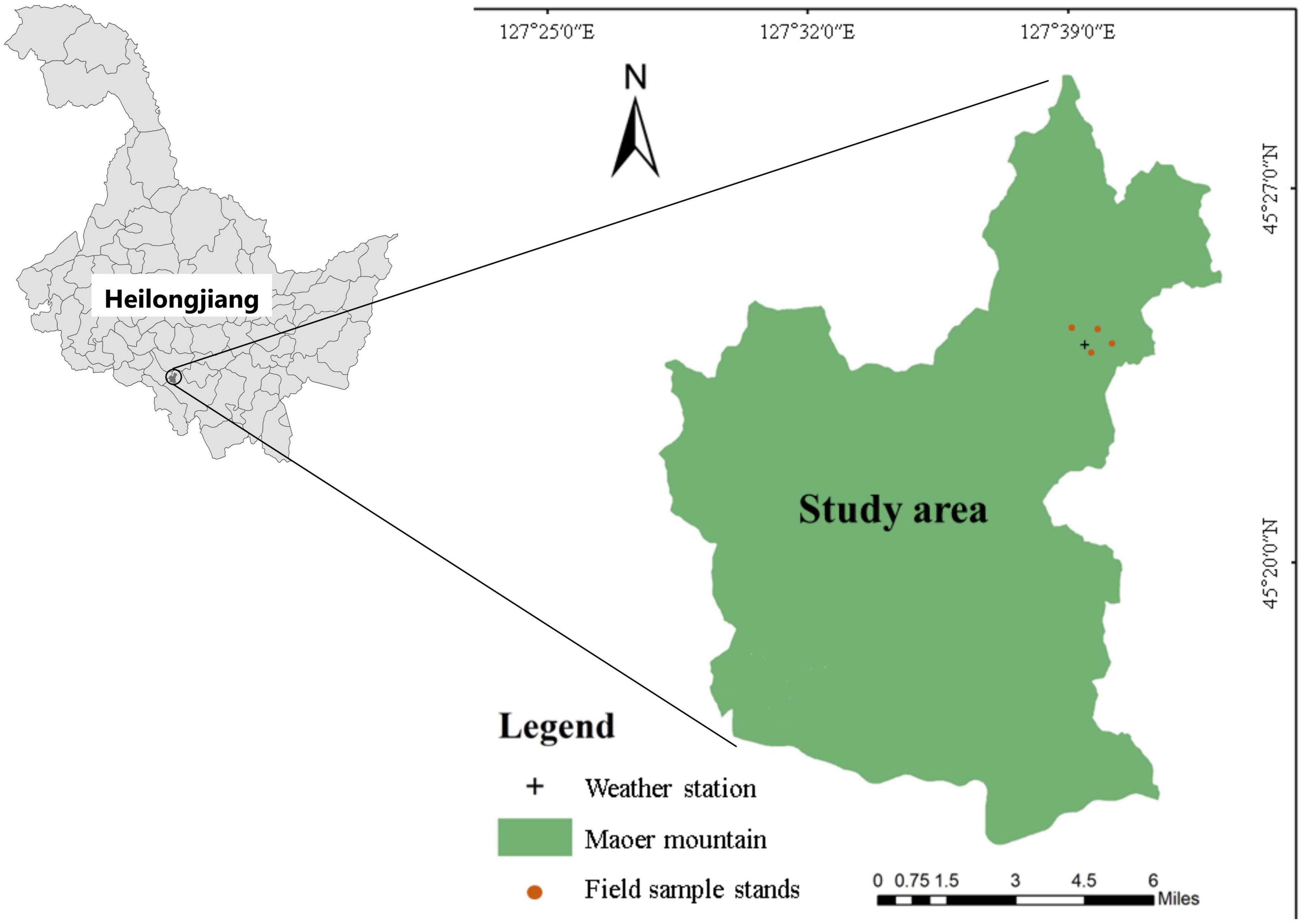
Figure 1. The location of the study area. The map on the right shows the location of four field sample stands.

2.2. Field experiment

We selected the plantations of these four typical forest types, and their surface litter was taken as the research object. The plantations of four typical forests in the study area were selected as the field sample stands, and 50 m × 50 m standard stands were set up and explored in each forest from 5 September to 10 September 2018 (the sample stand information is shown in Table 1). Five sampling points were uniformly set up in each sample stand by the random distribution method, and placed the FMC meter to collect the moisture content and meteorological data, which represents this forest by the average of all sampling points.

TABLE 1

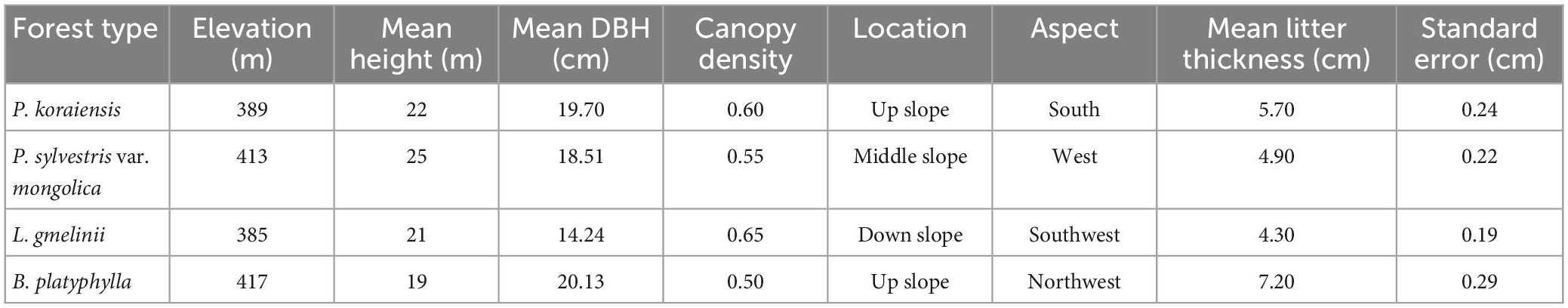
Table 1. The information of sample stands.

We used the fuel moisture content meter to continuous, automated measure real-time FFMC and meteorological data at half-hour intervals from 15 September to 15 November 2018 (covers the full fall fire season). The meter can monitor the FFMC in real time and has the function of a mini weather station, which is an automatic piece of weighing equipment continuously powered by batteries and solar energy (Masinda et al., 2021, 2022). It can automatically measure fuel mass, temperature, relative humidity, wind speed and solar radiation at regular intervals. To ensure its accuracy, before the measurement, we use weights (100 g, 200 g, and 500 g) to calibrate the values obtained by meter (error 0.01 g). The following is the specific use process. The meters were placed at the sample point in each forest type, collect the surface dead fine fuels near the sample point, take it back to the laboratory to dry and weigh it, and record the weight as the dry weight of the fuels. Put the collected fuels in a 30 cm × 30 cm × 6 cm basket, cover its upper surface with stainless steel net to prevent the fuels from falling. Before that, Weigh the basket and stainless steel net, the amount of water they absorb is negligible because their poor water absorption. After calibrating the meter, placed the basket back in the plot on the ground, and attached it to the meter. The meter weights the basket at half-hour intervals to calculate FFMC. At the same time of weighing, the temperature, relative humidity, wind speed, and solar radiation were measured and recorded 1 m above the ground. The precipitation data were collected from a nearby stationary weather station (within 2 km from the sampling point). We can transmit data and change the settings of meter through hotspot. During the experiment, there are a small portion of the data was lost due to the problems of the equipment itself or lack of electricity, we model and analyze the remaining data.

2.3. Data analysis

2.3.1. Basic statistics

For the data of P. koraiensis, P. sylvestris var. mongolica, L. gmelinii, and B. platyphylla, 1,121, 2,118, 2,310, and 1,367 data records were collected, respectively, during the study period. First, basic statistical analysis was performed on the collected data, and the FFMC and the maximum, minimum and average values of meteorological factors and FFMC in each forest were calculated. Taking the sampling date as abscissa and the dead FFMC as ordinate, the moisture content dynamic change of each forest type was plotting, and its driving factors were analyzed.

2.3.2. Prediction model

We use five different methods to build semi-physical models, machine learning models and linear regression model separately to predict FFMC. Previous studies have applied these five models and concluded that they are suitable for predicting FFMC with relatively high accuracy (Catchpole et al., 2001; Matthews, 2006; Lee et al., 2020; Zhang and Sun, 2020; Masinda et al., 2021, 2022). In this study, 70% of the data were used to train the model, and the remaining 30% were used to test and compare model performance. Each model is described below.

2.3.2.1. Semi-physical model

The direct time lag method considers the physical process of moisture diffusion of fuels, and the relevant parameters are obtained through experiments, which belongs to semi-physical model (Catchpole et al., 2001; Jin and Chen, 2012). And it is simple and accurate to use. It can accurately estimate FFMC in a short time interval by using real-time moisture content data and meteorological data obtained in the field, which has good applicability. It is one of the most widely used methods at present. To make the results more accurate, the Nelson model (Nelson, 1984) based on semi-physical and the Simard model (Simard, 1968) based on statistics were selected as the EMC response equations in the direct time lag method (hereinafter, they are simply referred to as the Nelson method and Simard method).

This method is mainly based on the differential equation of surface fuel moisture content proposed by Byram and Nelson (1963), as shown in Eq. (1):

$\frac{dM}{dt}=\frac{E-M}{\mathrm{\tau }}(1)$

Where M indicates the fine fuel moisture content (%), E is the equilibrium moisture content (%), and τ represents the time lag (h).

The Byram moisture differential Eq. (1) is discretized, and the following equation is obtained.

$\text{M}\left({\text{t}}_{\text{i}}\right)={\mathrm{\lambda }}^2{M}_{i-1}+\mathrm{\lambda }\left(1-\mathrm{\lambda }\right)E_{i-1}+\left(1-\mathrm{\lambda }\right)E_i(2)$

Where M(t_i) is the FFMC at time t_i, (%); M_i–1 is the FFMC at time t_i–1 (%); E_i is the equilibrium moisture content at time t_i, (%); E_i–1 is the equilibrium moisture content at time t_i–1, (%); λ is parameters of the model that were estimated according to the least square method, λ = exp[-δt/(2τ)]; τ = -δt/(2lnλ); and the Δt refers the time step in our study, so Δt = 0.5 h. The semi-physical models were implemented using the “tidyverse” package in R.

The equilibrium moisture content in the above formula is calculated either by the Nelson model or by the Simard model. The Nelson equilibrium moisture content model is shown in Eq. (3):

$E=\mathrm{\alpha }+\beta \log \mathrm{\Delta }G=\mathrm{\alpha }+\beta \log \left(-\frac{RT}{m}\log H\right)(3)$

Where R is the universal gas constant with a value of 8.314 J⋅K^–1⋅mol^–1; T is the air temperature (K); H is the relative humidity (%); m is the relative molecular mass of H₂O, with a value of 18 g⋅mol^–1; α and β are parameters of the model that were estimated according to the least square method.

The Simard equilibrium moisture content model is shown in Eq. (4):

$E=\{\begin{array}{c}0.03+0.626H-0.00104HT H<10 \\ 1.76+0.1601H-0.0266T \hspace{0.17em}\hspace{0.17em}10\le H<50\\ 21.06-0.4944H+0.005565H^2-0.00063HT H\ge 50\end{array}(4)$

Where E is equilibrium moisture content (%), T is air temperature (°C), and H is relative humidity (%).

2.3.2.2. Random forest

Random Forest is an integrated learning algorithm based on decision trees, which can describe linear and non-linear relationships without any additional assumptions about independent or dependent variables (Breiman, 2001; Kamińska, 2019). RF uses the bootstrap resampling method to extract multiple samples from the original sample, carries on decision tree modeling to each bootstrap sample, then combines the prediction of multiple decision trees, and obtains the final prediction result through voting (Gigoviæ et al., 2019). RF can overcome the complex non-linearity among many factors and different dimensions of data, which has high prediction accuracy. It has a faster learning speed than bagging and boosting, good tolerance to outliers and noise. In addition, many researches have used RF for predicting FFMC and have shown excellent performance (Lee et al., 2020; Fan and He, 2021; Masinda et al., 2021). The number of parameters that require tuning in RF is relatively small, namely the number of trees to grow (ntree) and the number of predictive variables (mtry) for segmenting nodes at each node (Lee et al., 2020). The ntree was set to 1,500, as recommended by Kuhn and Johnson (2013). In order to determine the best value of mtry, we made continuous attempts starting from 2, comparing the root mean square error (RMSE), mean absolute error (MAE) and R² value of the models, and finally got the best model. The importance and significance of independent variables in the model were quantitatively analyzed. The RF models were implemented using the “randomForest” package and the “rfPermute” package in R.

2.3.2.3. Generalized additive model

The generalized additive model is a semiparametric extension of the generalized linear model (GLM), which is a machine learning model. It is a non-parametric regression model driven by data rather than a statistical distribution model. GAM establishes the relationship between the mathematical expected value of the response variable and the smooth function of the explanatory variable by the link function (Gomez-Rubio, 2018). The advantage of the GAM is that many different link functions can be used to fit the non-linear and non-monotonic relations between response variables and multiple explanatory variables (Masinda et al., 2021). It can explain how the response variables (qualitative or semiquantitative discontinuous variables) change with the explanatory variables, and there is no need to set the model parameters in advance (Guisan et al., 2002). Therefore, GAM has a high degree of flexibility and can effectively reveal the ecological relationship hidden in the data. It can simply fit the non-linear relationship between multiple meteorological factors and FFMC, and concourse them in one model. Moreover, Masinda et al. (2021) also showed that it had similar accuracy to RF in predicting FFMC. The model is as follows:

$\text{n}=\text{g}\left(\mathrm{\mu }\right)={\text{s}}_0+\sum _{\text{i}=1}^{\text{p}}{\text{s}}_{\text{i}}\left({\text{x}}_{\text{i}}\right)(5)$

Where μE(Y|x₁,x₂x_p), n is a linear predictive value, s₀ is an intercept, s_i(⋅) is a non-parametric smooth function, x_i is an independent variable and s_i(x_i) is a smooth term. The model does not need any assumption of Y on x and consists of random component Y, additive component n and the link function s_i(⋅).

Because GAM is an “additive” assumption, the important interaction x_jx_k may be missing from the model and can only be added manually (Wood et al., 2013). In this study, the GAM is built by generalized cross-validation (GCV) method and restricted maximum likelihood (REML) method, respectively, and the two methods are compared by R² value and explanatory power. The GAM is implemented using the “mgcv” package in R.

2.3.2.4. Linear regression model

The linear regression model is an empirical model. The meteorological factors that have a significant influence on the FFMC are analyzed by forward stepwise regression analysis, and the regression model is built, as shown in Eq. (6):

$\text{M}=\sum _{\text{i}=1}^{\text{n}}{\text{x}}_{\text{i}}{b}_{\text{i}}(6)$

Where M is the FFMC, x_i is the selected meteorological factor, and b_i is the parameters to be estimated. The LR were implemented using the “tidyverse” package in R.

2.3.3. Model evaluation and comparison

Statistical analysis was carried out on each group of data. The normality of data distribution, the uniformity of variance, the independence of residuals and the consistency of model explanatory variables were tested. For checking the accuracy of the models built by the above methods, the MAE and RMSE of the models were calculated, as shown in Eqs. (7) and (8).

$\text{MAE}=\frac{1}{\text{n}}\sum _{\text{i}=1}^{\text{n}}\left|{\text{M}}_{\text{i}}-\widehat{{\text{M}}_{\text{i}}}\right|(7)$

$\text{RMSE}=\sqrt{\frac{1}{\text{n}}\sum _{\text{i}=1}^{\text{n}}{({\text{M}}_{\text{i}}-\widehat{{\text{M}}_{\text{i}}})}^2}(8)$

Where M_i is the measured value of FFMC (%) and $\widehat{M_i}$ is the predicted value of FFMC (%).

3. Results

3.1. Dynamic change in FFMC

The statistics of surface dead FFMC of the four forest types are shown in Table 2. The average value and variation range of FFMC in P. sylvestris var. mongolica were the largest, with a maximum value of 39.2%, a minimum value of 9.8% and an average value of 23.2%; the variation range in B. platyphylla was the smallest, with a maximum value of 30.8% and a minimum value of 9.4%; and the average value in P. koraiensis was the smallest, with a value of 19.8%.

TABLE 2

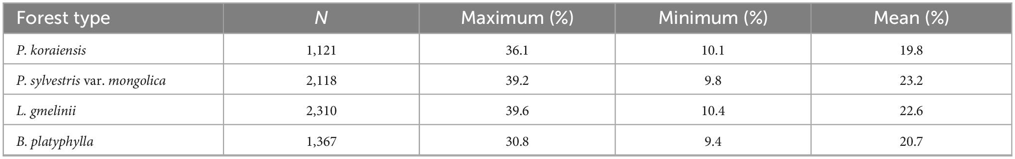
Table 2. Statistics on the moisture content of surface dead fuels in different forest stands.

The dynamic change trend of FFMC in each forest type was similar, showing characteristics of rising at first, then decreasing, and then rising (Figure 2). Except for B. platyphylla, the first peak occurred around September 29, which was due to rainfall during this period. Then, the FFMC gradually decreased and was usually less than 20% during the period from October 6 to October 19, returning to the normal level. Within this period, there was another small rainfall event in both P. sylvestris var. mongolica and L. gmelinii around October 9, which led to a small upward trend. After October 19, it showed an upward trend due to snow and reached its peak for the second time around October 20. The FFMC dynamic change of B. platyphylla was slightly later than that of the other forests, and the FFMC increased gradually on September 25, reached the first peak on October 3, and then decreased gradually until it showed an upward trend around October 16, and then the moisture content remained relatively stable.

FIGURE 2

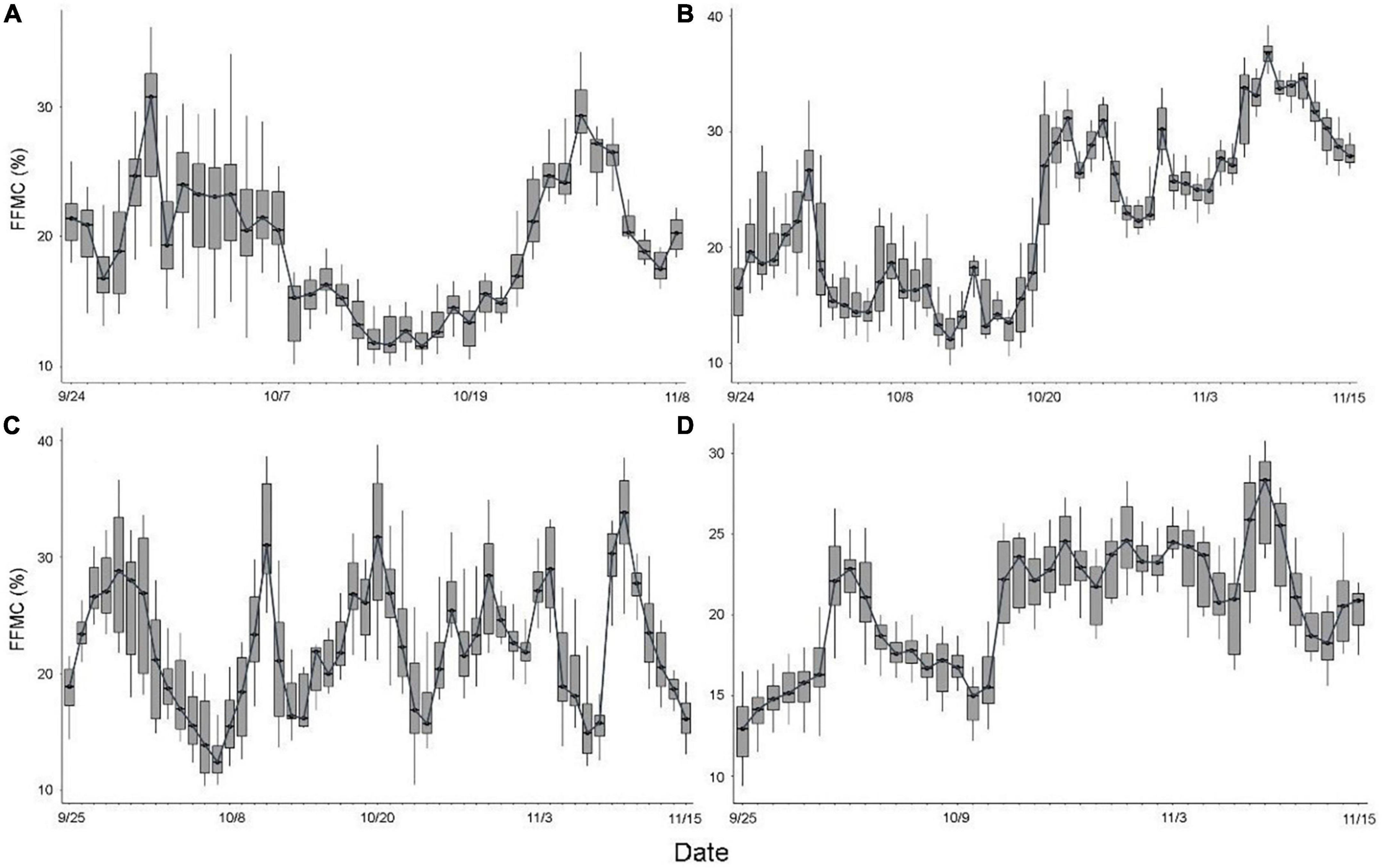
Figure 2. The dynamic change trend of fuel moisture content under different forest stands. (A) P. koraiensis fuel; (B) P. sylvestris var. mongolica fuel; (C) L. gmelinii fuel; and (D) B. platyphylla fuel.

3.2. The influence of meteorological factors

The Random Forest model was used to rank the importance of meteorological factors in different forests (Figure 3). In all forest types, temperature, relative humidity and radiation had significant effects (P < 0.01) on FFMC, the importance of temperature and relative humidity in all forests was greater than that of other factors. Rainfall had a significant effect on FFMC in all forest types, but the significance level was different (P < 0.05 in P. koraiensis, P < 0.01 in others). Wind had a significant effect (P < 0.01) on FFMC in P. koraiensis and B. platyphylla but not in the L. gmelinii forest. In summary, due to the difference in forest structure and the existence of spatial heterogeneity, meteorological factors have different effects on each forest. The temperature and relative humidity are the main meteorological factors affecting surface dead FFMC.

FIGURE 3

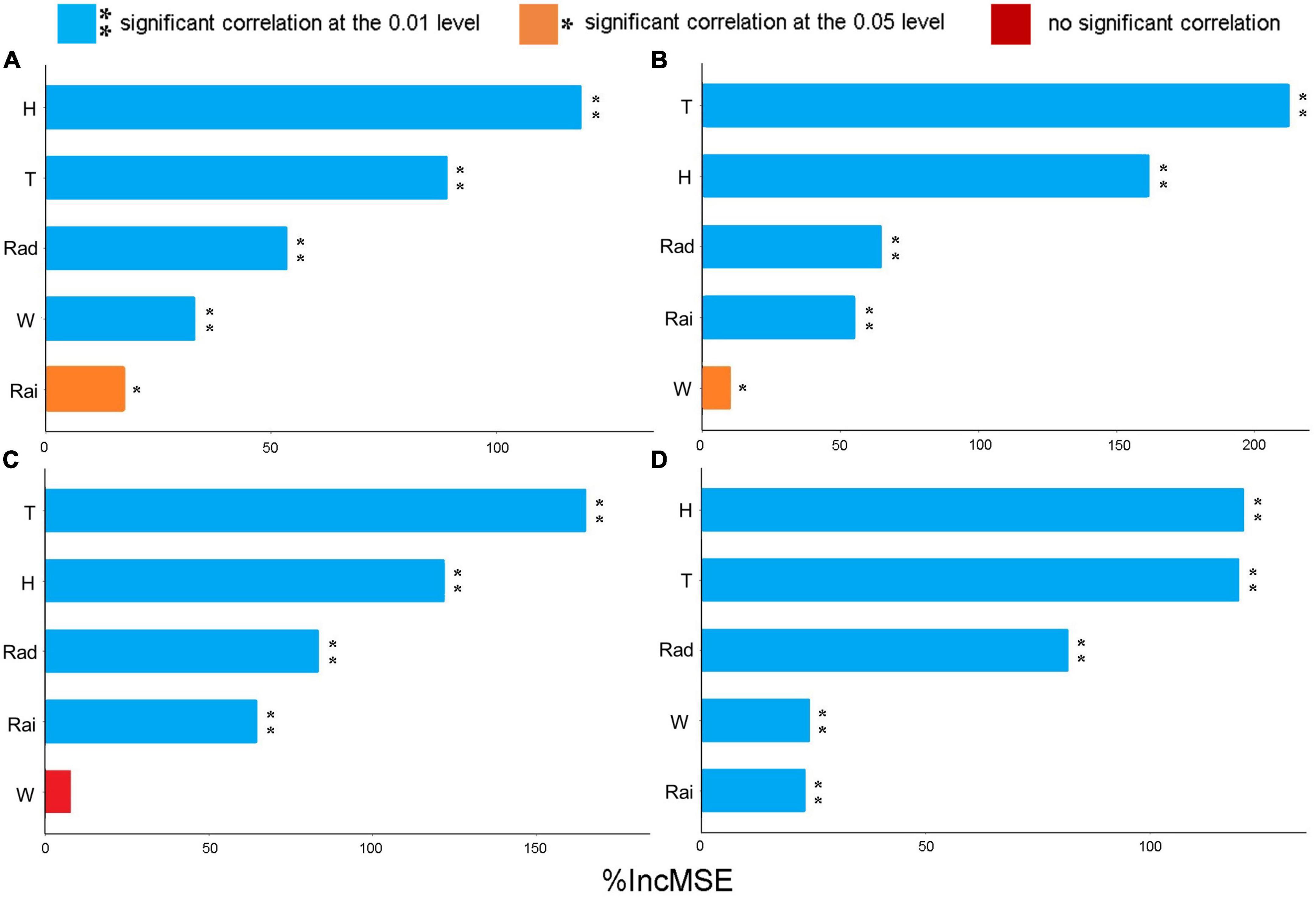
Figure 3. Variable importance measures with the Random Forest method based on mean squared error. T is temperature, H is relative humidity, Rai is rainfall, W is wind speed, and Rad is solar radiation; **indicates a significant correlation at the 0.01 level, *indicates a significant correlation at the 0.05 level; (A) P. koraiensis fuel; (B) P. sylvestris var. mongolica fuel; (C) L. gmelinii fuel; and (D) B. platyphylla fuel.

3.3. Model

3.3.1. Model parameters

3.3.1.1. Semi-physical models

In P. koraiensis, P. sylvestris var. mongolica, L. gmelinii and B. platyphylla, for Nelson method, the R² of the prediction models are from 0.853 to 0.980, and the time lags are 5.193 h, 35.589 h, 20.708 h, and 41.542 h, respectively; for Simard method, the R² of the prediction models are from 0.847 to 0.980, and the time lags are 27.635 h, 83.208 h, 35.589 h, and 124.875 h, respectively (Table 3). All models showed good performance, and the R² values of the three forests are approximately 0.970, except P. koraiensis. The time lag is related to the change rate of FFMC, and the larger the time lag is, the slower the change rate. For the four forests, the time lag of the Simard method was higher than that of the Nelson method, and the time lags of the two methods were in the following descending order for the four forests: B. platyphylla, P. sylvestris var. mongolica, L. gmelinii and P. Koraiensis.

TABLE 3

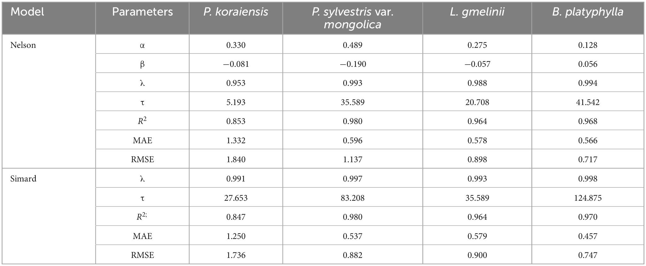
Table 3. Estimated parameters and goodness-of-fit-statistics of the Nelson model and Simard model.

3.3.1.2. Random forest

The number of variables tried at each split (mtry) can affect the model performance to some extent. Through continuous attempts, it was found that for all forests, when mtry was 4, the training and verification effect was the best, so mtry was determined to be 4 (Table 4). In all forests, the R² of the prediction models built by RF ranged from 0.903 to 0.935.

TABLE 4

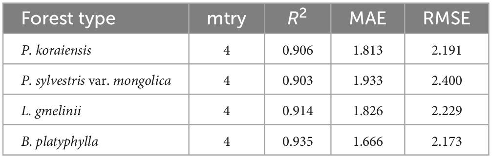
Table 4. Parameters and goodness-of-fit-statistics of the Random Forest model.

3.3.1.3. Generalized additive model

The estimated parameters and degrees of freedom of GAM in four forests are shown in Table 5 (GCV method) and Table 6 (REML method). In P. koraiensis, P. sylvestris var. mongolica, L. gmelinii, and B. platyphylla, for the GCV method, the R² of each forest was 0.267, 0.319, 0.235, and 0.350, respectively, and the explanatory power was 29.5, 31.9, 25.3, and 36.2%, respectively. For the REML method, the R² of each forest was 0.261, 0.313, 0.228, and 0.346, respectively, and the explanatory power was 28.5, 31.2, 24.3, and 35.4%, respectively. The performance of the models was relatively poor. Comparing R² and the explanatory power, it can be concluded that the GCV method showed a better performance than the REML method. Therefore, the GAM built by the GCV method was selected for the following research (all the GAMs mentioned below are built by the GCV method).

TABLE 5

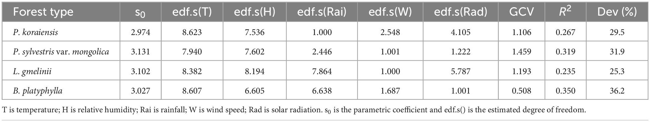
Table 5. Model parameters and degrees of freedom of smoothing terms with the GCV method.

TABLE 6

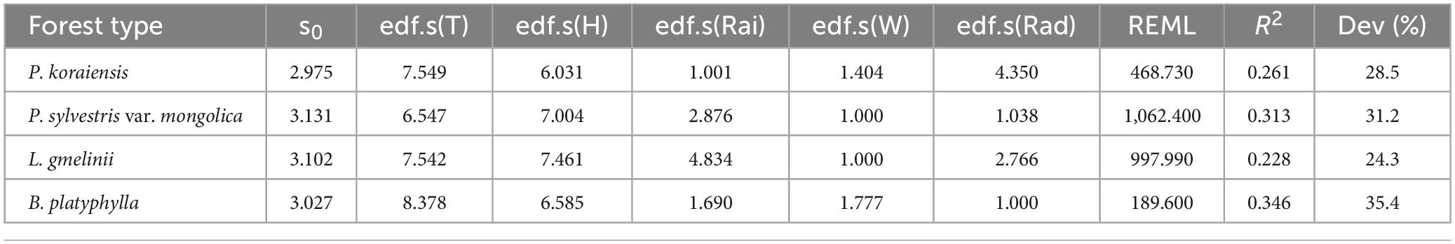
Table 6. Model parameters and degrees of freedom of smoothing terms with the REML method.

The greater the degree of freedom of the smooth term in the GAM, the more significant the non-linear relationship between the explanatory variable and the response variable. The degrees of freedom of temperature and relative humidity in all forests are significantly larger than those of the other three explanatory variables, so the non-linear relationship between them and FFMC was the most significant. The GCV value is one of the parameters used to evaluate the smoothness of the model; the smaller the value, the higher the smoothness of the model and the better the fitness. The GCV values from low to high were in the following order for the four forests: B. platyphylla, P. koraiensis, L. gmelinii, and P. sylvestris var. mongolica. The goodness-of-fit-statistics of GAM is shown in Table 7.

TABLE 7

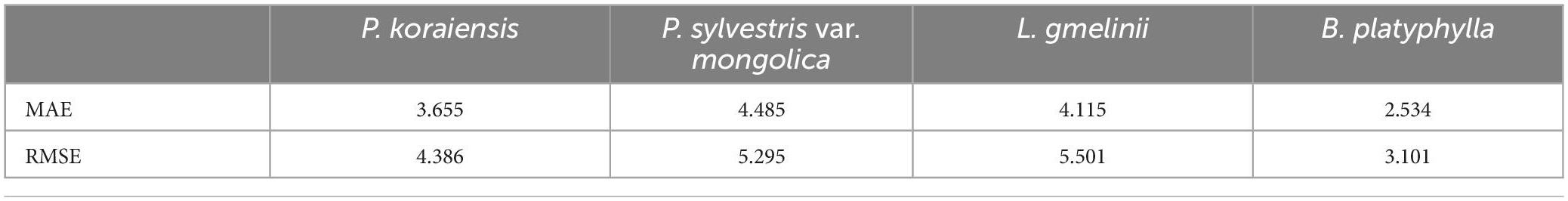
Table 7. The goodness-of-fit-statistics of generalized additive model.

3.3.1.4. Linear regression model

Linear regression models were developed using forward stepwise selection to screen the meteorological factors and build the best model. The results are shown in Table 8, for all forests, temperature, relative humidity and rainfall were all selected as the meteorological factors of the model. In addition, the P. koraiensis, also selected wind as the meteorological factors of the model, and the P. sylvestris var. mongolica and L. gmelinii also selected radiation as the meteorological factors of the model. The R² for the prediction models ranged from 0.147 to 0.244.

TABLE 8

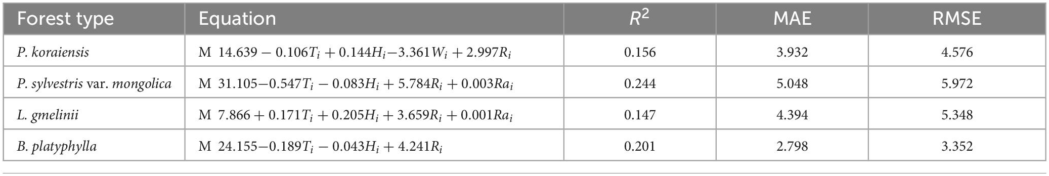
Table 8. Parameters and goodness-of-fit-statistics of the linear regression models.

3.3.2. Model error comparison

After building the prediction models based on the training data, the performance of the models were evaluated by the test data, and the model error was calculated based on test data. The MAE and RMSE of the models built by different methods in each forest are compared, as shown in Figure 4. For the Nelson method, the model error (MAE and RMSE) range was 0.566–1.840%; for the Simard method, the model error range was 0.457–1.736%; for the RF, the model error range was 1.666–2.400%; for the GAM, the model error range was 2.534–5.501%; and for the LR, the model error range was 2.798–5.972%.

FIGURE 4

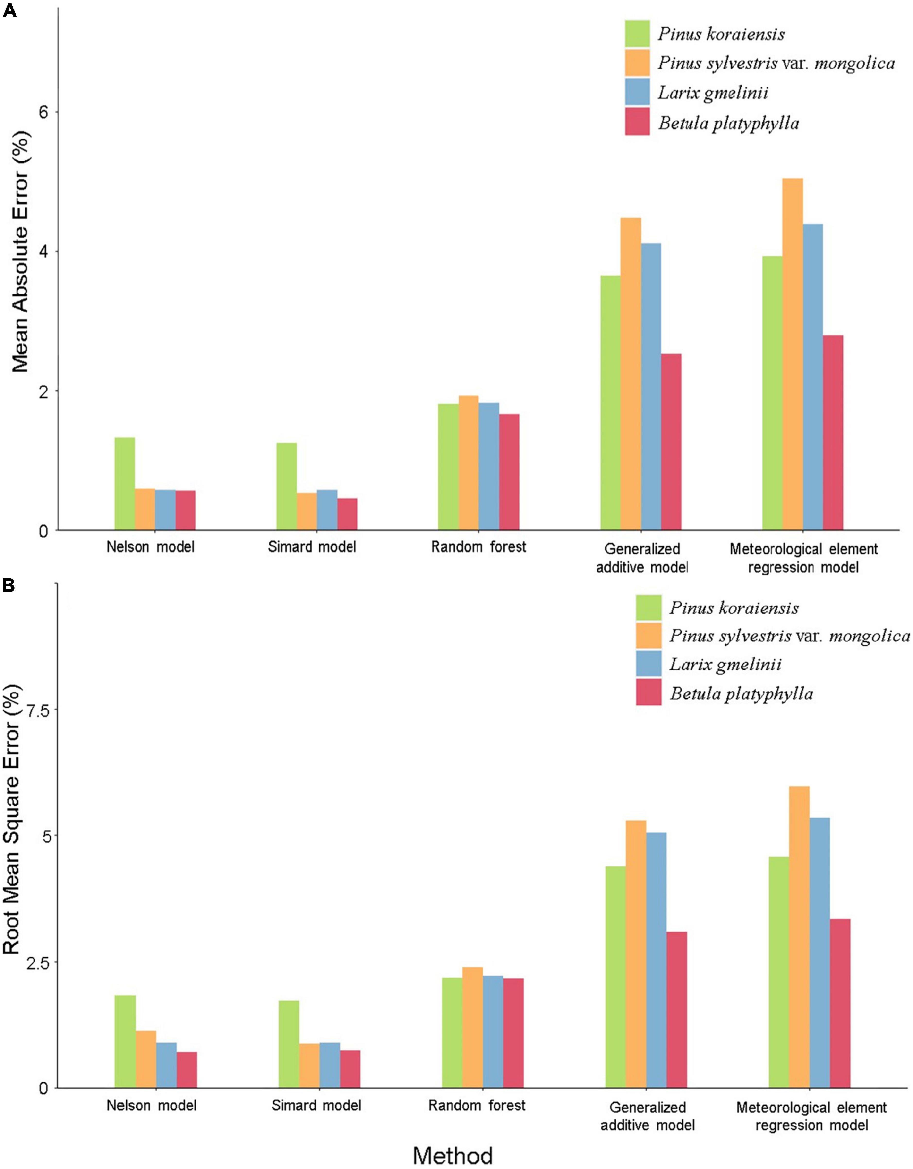
Figure 4. Comparison of fuel moisture content model errors in each forest. (A) Mean absolute error (%). (B) Root mean square error (%).

Comparing the accuracy for different forests in the same method, for the RF, GAM, and LR, the accuracy of the prediction model in each forest from high to low was B. platyphylla, P. koraiensis, L. gmelinii, and P. sylvestris var. mongolica. For the Nelson method and Simard method, the accuracy of the prediction model was the highest in B. platyphylla, the second highest in P. sylvestris var. mongolica and L. gmelinii and the lowest in P. koraiensis. In general, no matter which method was used, the accuracy of the prediction model in B. platyphylla was the highest among all forests.

Comparing the accuracy of different methods in the same forest, the accuracy of GAM and LR was significantly lower than that of the other methods, their model errors are relatively large, and GAM was slightly better than LR. The Nelson method, Simard method and RF show good performance, and the model errors in most forests are all less than 2%, which was significantly higher than those of GAM and LR. For the these three methods, in P. koraiensis, P. sylvestris var. mongolica, and B. platyphylla, the accuracy of the Simard method was the highest, the Nelson method was the second highest, and the RF method was the lowest in L. gmelini, the accuracy of the Nelson method was the highest, the Simard method was the second highest, and the RF method was also the lowest. Moreover, the prediction accuracy of the Nelson method and Simard method was very close in all forests. In general, the Nelson method and Simard method which belong to the semi-physical model perform better than the Random Forest method which belongs to the machine learning model.

3.3.3. Model performance evaluation

Compared with the other three methods, the prediction performance of GAM and LR was significantly lower, so they are not studied below. The measured values of the test data were compared with the predicted values obtained from the Nelson method, Simard method and RF built based on the training data, as shown in Figure 5. In all forests, the predicted values of the Nelson method and Simard method are basically consistent with the measured values, the R² of the fitting lines ranged from 0.881 to 0.984, and the accuracy of the Simard method was slightly better than that of the Nelson method. For the RF, there was a certain deviation between the predicted and measured values in all forests, the R² of the fitting lines ranged from 0.607 to 0.864, and the model overestimated when the FFMC was lower than ∼21% but underestimated when it was higher than ∼21%, especially in B. platyphylla. Therefore, we can consider that the prediction accuracy of RF was slightly lower than that of the other two methods. In summary, the accuracy of the five methods in all forests from high to low was ranked as follows: Simard method > Nelson method > RF > GAM > LR.

FIGURE 5

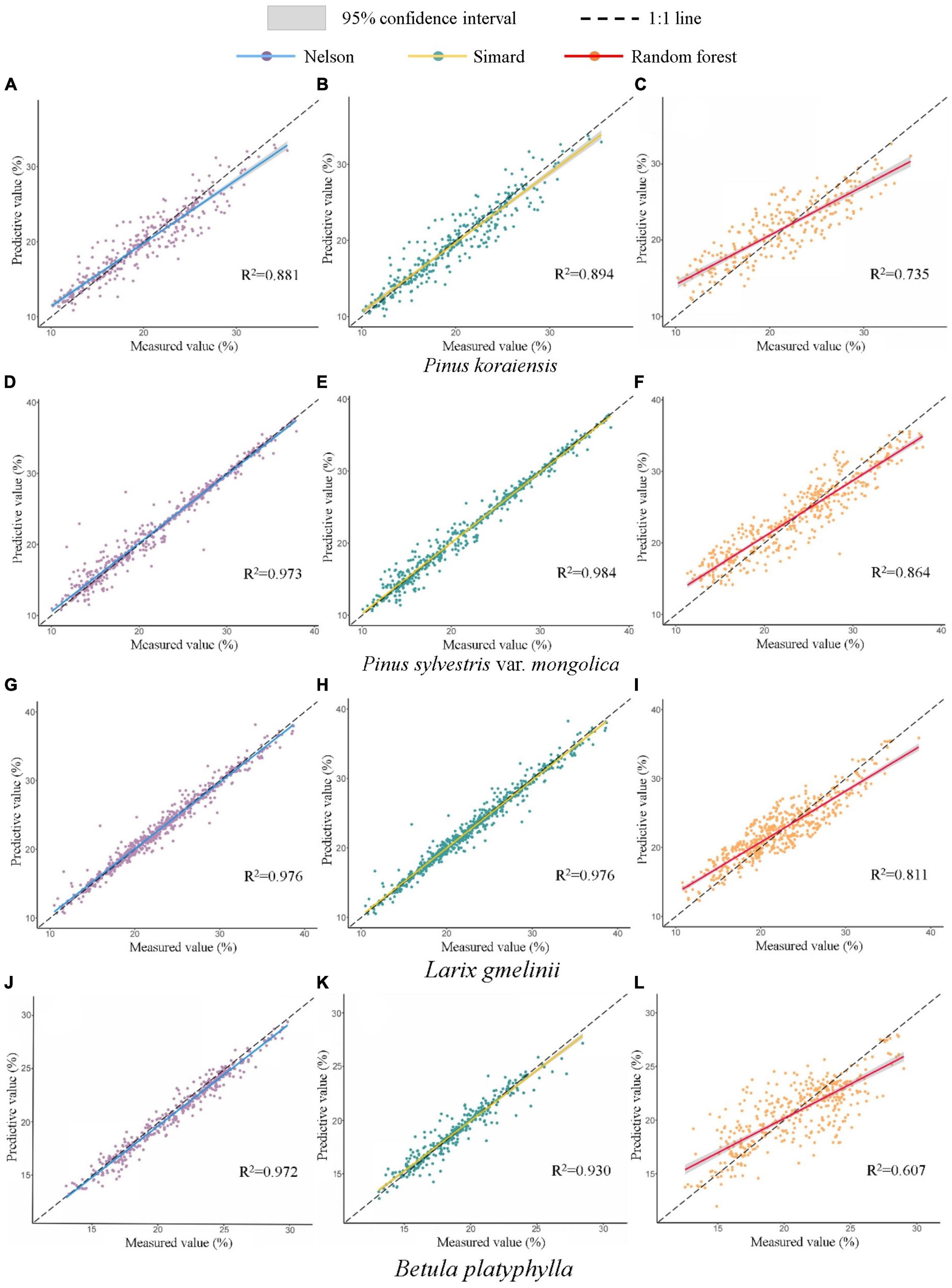
Figure 5. 1:1 Error scatter plot of the predicted and measured values of each forest. (A–C) P. koraiensis fuel; (D–F) P. sylvestris var. mongolica fuel; (G–I) L. gmelinii fuel; (J–L) B. platyphylla fuel.

4. Discussion

4.1. Meteorological factor analysis

The quantitative analysis of the importance of meteorological variables by RF model showed that temperature, relative humidity and solar radiation had significant effects on FFMC in all forests, especially temperature and relative humidity, and their importance was greater than that of the other three meteorological factors. The result is similar to those of previous studies (Viney, 1991; Slijepcevic et al., 2013; Nyman et al., 2015; Zhang et al., 2017; Masinda et al., 2021; Yu et al., 2021), temperature and relative humidity are the most important meteorological factors, which directly affect the FFMC. The effect of wind on the FFMC is affected by topography, forest structure, crown density and so on. In this study, only the surface dead FFMC in P. koraiensis and B. platyphylla was significantly affected (P < 0.01) by wind, which was similar to the results of Bilgili et al. (2019) and Zhang and Sun (2020). This is because the time interval of wind speed data collection during the study period was short, which could not reflect the impact of wind on FFMC. In addition, it underestimates the effect of rainfall on FFMC, which is the same as the results of Masinda et al. (2021). This may be because the rainfall and duration were short, and most of the data collected were zero, so their importance was not reflected.

4.2. Model parameters

In the semi-physical models, the parameters of the Nelson equilibrium moisture content model need to be estimated according to the experimental data. In P. koraiensis, P. sylvestris var. mongolica, L. gmelinii, and B. platyphylla, the α values are 0.330, 0.489, 0.275, and 0.128, respectively, and the β values are −0.081, −0.190, −0.057, and 0.056, respectively. This is similar to the results of previous studies, Sun et al. (2015) found that the α-value ranged from 0.087 to 0.594, Slijepcevic et al. (2013) found that the α-value ranged from 0.28 to 0.41. Zhang and Sun (2020) found that the α values of P. koraiensis and Quercus mongolica were 0.0039 and 0.2458, respectively. In addition to the influence of the type of fuel, the reason for the difference is also related to the measuring methods and time step. In most previous studies, the shortest time step was 1 h, but we measured the moisture content data of the whole autumn fire season with half-hour steps. The value of β can directly reflect the sensitivity of equilibrium moisture content to temperature and humidity; the greater the absolute value of β is, the stronger the sensitivity of fuels to temperature and humidity and the weaker the water holding capacity of fuels (Nelson, 1984). In this study, the absolute value of β from high to low resulted in the following order for the four forests: P. sylvestris var. mongolica, P. koraiensis, L. gmelinii, and B. platyphylla; that is, the water holding capacity of the broad-leaf layer is stronger than that of the needle layer. This is different from the results of Zhang and Sun (2020) and Yu et al. (2021). The reason is that the different fuel types and sampling seasons affect the structural characteristics, such as the physical and chemical properties of fuels and packing ratio of the litter bed, which lead to different results.

4.3. Model evaluation and comparison

Five different methods were used to build the prediction model of surface dead FFMC of each forest, and the accuracy and applicability of the model were evaluated based on the test data. The value of R² reflects the goodness-of-fit of different models in each forest type. For Nelson method and Simard method, their values of R² were very similar, except P. koraiensis was about 0.850, the other three forest types were all about 0.970, which shows that the regression line fits the observed values very well. For RF, its R² ranged from 0.903 to 0.935, which is similar to the above two methods and also shows a good goodness-of-fit. However, the R² ranges of GAM and LR are 0.235–0.350 and 0.147–0.244, respectively, which are significantly lower than the other three methods, so their fitting degree is poor and the accuracy is low. By comparing the model errors, it can be concluded that no matter which method is used, the accuracy of the prediction model in B. platyphylla is the highest among all forests. This is because B. platyphylla belongs to the broad-leaved tree, its leaves are small and flat, and the structure of the fuel bed is simpler and more uniform than that of needles, so the same method shows better accuracy, which is similar to the research results of Yu et al. (2021).

The accuracy of different methods has been compared. Among all forests, the accuracy of the five methods from high to low was ranked as follows: Simard method > Nelson method > RF > GAM > LR. The Nelson method and Simard method based on the direct time lag method have the highest accuracy, which may be related to the short time interval (half an hour) of data collection in this study (de Groot and Wang, 2005; Matthews, 2010, 2014). The results were similar to most previous studies, and the prediction accuracy of the Simard method is slightly better than that of the Nelson method (Jin and Chen, 2012; Sun et al., 2015; Zhang and Sun, 2020). Although both RF and GAM belong to machine learning algorithms, their theories are different (Breiman, 2001; Gomez-Rubio, 2018; Kamińska, 2019), so the accuracy of the prediction model shows an obvious difference. The performance of RF is significantly better than that of GAM, it is more suitable for FFMC prediction (Lee et al., 2020; Masinda et al., 2021). However, its accuracy was still slightly lower than that of Nelson method and Simard method. As shown in Figure 5, RF has underestimated large values and overestimated small values. This is due to its own principles, RF tends to intermediate predicted values, the extreme observations are estimated using averages of response values that are closer to those observations (Zhang and Lu, 2012; Wolfensberger et al., 2021). The result of LR is similar to the GAM, which is significantly lower than that of the other three methods (Sun et al., 2015; Masinda et al., 2021; Yu et al., 2021). Because they are based on the linear or non-linear relationship between FFMC and meteorological factors, the selection of meteorological factors has a great impact on the accuracy of the model. However, we did not consider the effects of soil moisture and previous meteorological factors in this study (Zhang and Sun, 2020; Lindberg et al., 2021; Rakhmatulina et al., 2021), which may be the reason for the large error values.

By and large, the semi-physical models (Nelson method and Simard method) have the highest accuracy, machine learning models perform slightly worse, and the linear regression model (LR) has the worst accuracy. The research of Lee et al. (2020) showed that for 10-h FFMC, the accuracy of machine learning is higher than that of process model, which is different from us. This is due to the difference sizes of the fuels, we took the fine fuels of 1-h as the research object, and its speed of water loss and water absorption is faster than that of 10-h fuels. One of the potential reasons for the highest accuracy of semi-physical models may be the short time interval, and the accuracy will decrease with the time interval increases in practical use (de Groot and Wang, 2005; Matthews, 2014; Zhang et al., 2021). Although the accuracy of the machine learning models is slightly lower, it can introduce new variables and data in the future to continuously develop the models, which has great potential to be widely used. However, there is another point deserve attention in machine learning models is the model cannot be described by formulas, which may have some limitations on future applications. Therefore, in future research, we should focus on the combination of data-driven (e.g., machine learning) and process-driven (e.g., physical and semi-physical models) methods proposed by Reichstein et al. (2019) to build hybrid models to achieve complementarity. In addition, more machine learning models should also be considered.

The prediction accuracy of FFMC must reach a MAE of approximately 1–2% to meet the accuracy requirements of fire risk prediction (Trevitt, 1991; Pippen, 2008). Our results showed that the model errors of the Simard method, Nelson method and RF in all forests are less than 2%. They were better than the MAE range from 0.8 to 1.9% reported by Catchpole et al. (2001), and the MAE and MRE (mean relative error) of 1.3 and 9.4%, respectively, reported by Matthews and McCaw (2006); and are similar to the research results of Zhang and Sun (2020) and Masinda et al. (2021). These three models can be used to predict FFMC of all four forests, and their accuracy can meet the requirements. Moreover, it also proven that the RF is also suitable for predicting FFMC, and its model has good performance. The GAM and LR have relatively large error values, which are not suitable. This study still has some limitations, for instance, not considering the season, the lag of meteorological factors and the effects of topographic conditions such as slopes and aspects on FFMC. In future research, we should fully consider the effects of different forest characteristics and topographical conditions on FFMC and its dynamic changes, which can provide theoretical support for improving the accuracy and applicability of the prediction of FFMC.

5. Conclusion

In this paper, the dynamic changes and main driving factors of surface dead FFMC of four typical forests in Northeast China were studied, five different methods were used to build models for predicting FFMC, and their performances were compared based on test data. The results showed that the dynamic change trends of FFMC in each forest were similar, and temperature and relative humidity were the main driving factors of FFMC. The model error and comparison of measured and predicted values showed that the semi-physical models (Nelson method and Simard method) perform best, the machine learning models (RF and GAM) perform slightly worse, and the linear regression model (LR) performs worst. Among them, the accuracy of the prediction models based on the Nelson method, Simard method and RF meet the requirements of forest fire risk prediction. The results of the model comparison in this study have reference value for the future research direction of the FFMC prediction model, as well as forest fire management and prediction in Northeast China.

Data availability statement

The raw data supporting the conclusions of this article will be made available by the authors, without undue reservation.

Author contributions

JF, LS, TH, and QL contributed to the conception and design of the study. JF and TH performed the data analysis, interpretation of results, and draft manuscript preparation. LS, JF, JR, and TH contributed to the critical revision of the manuscript. All authors reviewed the results and approved the final version of the manuscript.

Funding

This work was supported by the National Key Research and Development Program of China, the Key Projects for Strategic International Innovative Cooperation in Science and Technology (2018YFE0207800), the Youth Lift Project of China Association for Science and Technology (Grant No. YESS20210370), the Heilongjiang Province Outstanding Youth Joint Guidance Project (No. LH2021C012), and the Research and Development of Forest and Grassland Fire Early Prevention and Control System Platform.

Acknowledgments

We thank the Northern Forest Fire Management Key Laboratory of the National Forestry and Grassland Administration of P. R. China and the National Innovation Alliance of Wildland Fire Prevention and Control Technology of China for supporting this research.

Conflict of interest

The authors declare that the research was conducted in the absence of any commercial or financial relationships that could be construed as a potential conflict of interest.

Publisher’s note

All claims expressed in this article are solely those of the authors and do not necessarily represent those of their affiliated organizations, or those of the publisher, the editors and the reviewers. Any product that may be evaluated in this article, or claim that may be made by its manufacturer, is not guaranteed or endorsed by the publisher.

References

Aguado, I., Chuvieco, E., Borén, R., and Nieto, H. (2007). Estimation of dead fuel moisture content from meteorological data in Mediterranean areas. Applications in fire danger assessment. Int. J. Wildland Fire 16, 390–397. doi: 10.1071/WF06136

CrossRef Full Text | Google Scholar

Alves, M. V. G., Batista, A. C., Soares, R. V., Ottaviano, M., and Marchetti, M. (2009). Fuel moisture sampling and modeling in Pinus elliottii Engelm. plantations based on weather conditions in Paraná-Brazil. iForest 2, 99–103. doi: 10.3832/ifor0489-002

PubMed Abstract | CrossRef Full Text | Google Scholar

Andela, N., Morton, D. C., Giglio, L., Chen, Y., van der Werf, G. R., Kasibhatla, P. S., et al. (2017). A human-driven decline in global burned area. Science 356, 1356–1362. doi: 10.1126/science.aal4108

PubMed Abstract | CrossRef Full Text | Google Scholar

Artés, T., Oom, D., De Rigo, D., Durrant, T. H., Maianti, P., Libertà, G., et al. (2019). A global wildfire dataset for the analysis of fire regimes and fire behaviour. Sci. Data 6, 1–11. doi: 10.6084/m9.figshare.10284101

CrossRef Full Text | Google Scholar

Bar-Massada, A., and Lebrija-Trejos, E. (2020). Spatial and temporal dynamics of live fuel moisture content in eastern Mediterranean woodlands are driven by an interaction between climate and community structure. Int. J. Wildland Fire 30, 190–196. doi: 10.1071/WF20015

CrossRef Full Text | Google Scholar

Bilgili, E., Coskuner, K. A., Usta, Y., and Goltas, M. (2019). Modeling surface fuels moisture content in Pinus brutia stands. J. For. Res. 30, 577–587. doi: 10.1007/s11676-018-0702-x

CrossRef Full Text | Google Scholar

Bovill, W., Hawthorne, S., Radic, J., Baillie, C., Ashton, A., Lane, P., et al. (2015). “Effectiveness of automated fuelsticks for predicting the moisture content of dead fuels in Eucalyptus forests,” in Proceedings of the 21st international congress on modelling and simulation, 29 November–4 December 2015, Gold Coast, QLD, 201–207.

Google Scholar

Bowman, D. M., Kolden, C. A., Abatzoglou, J. T., Johnston, F. H., van der Werf, G. R., and Flannigan, M. (2020). Vegetation fires in the Anthropocene. Nat. Rev. Earth Environ. 1, 500–515. doi: 10.1038/s43017-020-0085-3

CrossRef Full Text | Google Scholar

Breiman, L. (2001). Random forests. Mach. Learn. 45, 5–32. doi: 10.1023/A:1010933404324

CrossRef Full Text | Google Scholar

Byram, G. M., and Nelson, R. M. (1963). An analysis of the drying process in forest fuel material. General technical report. Washington, DC: U.S. Department of Agriculture Forest Service, 1–38.

Google Scholar

Capps, S. B., Zhuang, W., Liu, R., Rolinski, T., and Qu, X. (2021). Modelling chamise fuel moisture content across California: A machine learning approach. Int. J. Wildland Fire 31, 136–148. doi: 10.1071/WF21061

CrossRef Full Text | Google Scholar

Catchpole, E. A., Catchpole, W. R., Viney, N. R., McCaw, W. L., and Marsden-Smedley, J. B. (2001). Estimating fuel response time and predicting fuel moisture content from field data. Int. J. Wildland Fire 10, 215–222. doi: 10.1071/WF01011

CrossRef Full Text | Google Scholar

Cawson, J. G., Nyman, P., Schunk, C., Sheridan, G. J., Duff, T. J., Gibos, K., et al. (2020). Estimation of surface dead fine fuel moisture using automated fuel moisture sticks across a range of forests worldwide. Int. J. Wildland Fire 29, 548–559. doi: 10.1071/WF19061

CrossRef Full Text | Google Scholar

Coker, E. S., Martin, J., Bradley, L. D., Sem, K., Clarke, K., and Sabo-Attwood, T. (2021). A time series analysis of the ecologic relationship between acute and intermediate PM2. 5 exposure duration on neonatal intensive care unit admissions in Florida. Environ. Res. 196:110374. doi: 10.1016/j.envres.2020.110374

PubMed Abstract | CrossRef Full Text | Google Scholar

da Silva Marques, D., Costa, P. G., Souza, G. M., Cardozo, J. G., Barcarolli, I. F., and Bianchini, A. (2019). Selection of biochemical and physiological parameters in the croaker Micropogonias furnieri as biomarkers of chemical contamination in estuaries using a generalized additive model (GAM). Sci. Total Environ. 647, 1456–1467. doi: 10.1016/j.scitotenv.2018.08.049

PubMed Abstract | CrossRef Full Text | Google Scholar

de Groot, W. J., and Wang, Y. (2005). Calibrating the fine fuel moisture code for grass ignition potential in Sumatra, Indonesia. Int. J. Wildland Fire 14, 161–168. doi: 10.1071/WF04054

CrossRef Full Text | Google Scholar

Ellis, T. M., Bowman, D. M., Jain, P., Flannigan, M. D., and Williamson, G. J. (2022). Global increase in wildfire risk due to climate-driven declines in fuel moisture. Glob Chang Biol. 28, 1544–1559. doi: 10.1111/gcb.16006

PubMed Abstract | CrossRef Full Text | Google Scholar

Fan, C., and He, B. (2021). A physics-guided deep learning model for 10-h dead fuel moisture content estimation. Forests 12:933. doi: 10.3390/f12070933

CrossRef Full Text | Google Scholar

Gigoviæ, L., Pourghasemi, H. R., Drobnjak, S., and Bai, S. (2019). Testing a new ensemble model based on SVM and random forest in forest fire susceptibility assessment and its mapping in Serbia’s Tara National Park. Forests 10:408. doi: 10.3390/f10050408

CrossRef Full Text | Google Scholar

Gomez-Rubio, V. (2018). Generalized additive models: An introduction with R. J. Stat. Softw. 86, 1–5. doi: 10.18637/jss.v086.b01

CrossRef Full Text | Google Scholar

González, A. D. R., Hidalgo, J. A. V., and González, J. G. (2009). Construction of empirical models for predicting Pinus sp. dead fine fuel moisture in NW Spain. I: Response to changes in temperature and relative humidity. Int. J. Wildland Fire 18, 71–83. doi: 10.1071/WF07101

CrossRef Full Text | Google Scholar

Gould, J. S., McCaw, W. L., and Cheney, N. P. (2011). Quantifying fine fuel dynamics and structure in dry eucalypt forest (Eucalyptus marginata) in Western Australia for fire management. For. Ecol. Manag. 262, 531–546. doi: 10.1016/j.foreco.2011.04.022

CrossRef Full Text | Google Scholar

Guisan, A., Edwards, T. C. Jr., and Hastie, T. (2002). Generalized linear and generalized additive models in studies of species distributions: Setting the scene. Ecol. Modell. 157, 89–100.

Google Scholar

Holsinger, L., Parks, S. A., and Miller, C. (2016). Weather, fuels, and topography impede wildland fire spread in western US landscapes. For. Ecol. Manag. 380, 59–69. doi: 10.1016/j.foreco.2016.08.035

CrossRef Full Text | Google Scholar

Jin, S., and Chen, P. (2012). Modelling drying processes of fuelbeds of Scots pine needles with initial moisture content above the fibre saturation point by two-phase models. Int. J. Wildland Fire 21, 418–427. doi: 10.1071/WF10119

CrossRef Full Text | Google Scholar

Jin, S., and Li, L. (2010). Validation of the method for direct estimation of timelag and equilibrium moisture content of forest fuel. Sci. Silvae Sin. 46, 95–105.

Google Scholar

Jolly, W. M., Cochrane, M. A., Freeborn, P. H., Holden, Z. A., Brown, T. J., Williamson, G. J., et al. (2015). Climate-induced variations in global wildfire danger from 1979 to 2013. Nat. Commun. 6, 1–11. doi: 10.1038/ncomms8537

PubMed Abstract | CrossRef Full Text | Google Scholar

Kamińska, J. A. (2019). A Random Forest partition model for predicting NO2 concentrations from traffic flow and meteorological conditions. Sci. Total Environ. 651, 475–483. doi: 10.1016/j.scitotenv.2018.09.196

PubMed Abstract | CrossRef Full Text | Google Scholar

Kang, Y., Jang, E., Im, J., Kwon, C., and Kim, S. (2020). Developing a new hourly forest fire risk index based on catboost in South Korea. Appl. Sci. 10:8213. doi: 10.3390/app10228213

CrossRef Full Text | Google Scholar

Kuhn, M., and Johnson, K. (2013). Applied predictive modeling. New York, NY: Springer. doi: 10.1007/978-1-4614-6849-3

CrossRef Full Text | Google Scholar

Lee, H., Won, M., Yoon, S., and Jang, K. (2020). Estimation of 10-hour fuel moisture content using meteorological data: A model inter-comparison study. Forests 11, 982. doi: 10.3390/f11090982

CrossRef Full Text | Google Scholar

Lei, W. D., Yu, Y., Li, X. H., and Xing, J. (2022). Estimating dead fine fuel moisture content of forest surface, based on wireless sensor network and back-propagation neural network. Int. J. Wildland Fire 31, 369–378. doi: 10.1071/WF21066

CrossRef Full Text | Google Scholar

Li, Y. (2021). Study on temporal and spatial variation of forest fire and fire risk prediction in large-scale areas. Ph.D. dissertation. Beijing: Beijing Forestry University.

Google Scholar

Lindberg, H., Aakala, T., and Vanha-Majamaa, I. (2021). Moisture content variation of ground vegetation fuels in boreal mesic and sub-xeric mineral soil forests in Finland. Int. J. Wildland Fire 30, 283–293. doi: 10.1071/WF20085

CrossRef Full Text | Google Scholar

Liu, N., Lei, J., Gao, W., Chen, H., and Xie, X. (2021). Combustion dynamics of large-scale wildfires. Proc. Combust. Inst. 38, 157–198. doi: 10.1016/j.proci.2020.11.006

CrossRef Full Text | Google Scholar

Masinda, M. M., Li, F., Liu, Q., Sun, L., and Hu, T. (2021). Prediction model of moisture content of dead fine fuel in forest plantations on Maoer Mountain, Northeast China. J. For. Res. 32, 2023–2035.

Google Scholar

Masinda, M. M., Li, F., Qi, L., Sun, L., and Hu, T. (2022). Forest fire risk estimation in a typical temperate forest in Northeastern China using the Canadian forest fire weather index: Case study in autumn 2019 and 2020. Nat. Hazards 111, 1085–1101. doi: 10.1007/s11069-021-05054-4

PubMed Abstract | CrossRef Full Text | Google Scholar

Matthews, S. (2006). A process-based model of fine fuel moisture. Int. J. Wildland Fire 15, 155–168. doi: 10.1071/WF05063

CrossRef Full Text | Google Scholar

Matthews, S. (2010). Effect of drying temperature on fuel moisture content measurements. Int. J. Wildland Fire 19, 800–802. doi: 10.1071/WF08188

CrossRef Full Text | Google Scholar

Matthews, S. (2014). Dead fuel moisture research: 1991–2012. Int. J. Wildland Fire 23, 78–92. doi: 10.1071/WF13005

CrossRef Full Text | Google Scholar

Matthews, S., and McCaw, W. L. (2006). A next-generation fuel moisture model for fire behaviour prediction. For. Ecol. Manag. 234:S91. doi: 10.1016/J.FORECO.2006.08.127

CrossRef Full Text | Google Scholar

Matthews, S., Gould, J., and McCaw, L. (2010). Simple models for predicting dead fuel moisture in eucalyptus forests. Int. J. Wildland Fire 19, 459–467. doi: 10.1071/WF09005

CrossRef Full Text | Google Scholar

Nelson, R. M. (1984). A method for describing equilibrium moisture content of forest fuels. Can. J. For. Res. 14, 597–600. doi: 10.1139/x84-108

CrossRef Full Text | Google Scholar

Nelson, R. M. (2000). Prediction of diurnal change in 10-h fuel stick moisture content. Can. J. For. Res. 30, 1071–1087. doi: 10.1139/X00-032

CrossRef Full Text | Google Scholar

Nyman, P., Metzen, D., Noske, P. J., Lane, P. N., and Sheridan, G. J. (2015). Quantifying the effects of topographic aspect on water content and temperature in fine surface fuel. Int. J. Wildland Fire 24, 1129–1142. doi: 10.1071/WF14195

CrossRef Full Text | Google Scholar

Palomino, A. F., Espino, P. S., Reyes, C. B., Rojas, J. A. J., and Silva, F. R. (2022). Estimation of moisture in live fuels in the mediterranean: Linear regressions and Random Forests. J. Environ. Manage 322, 116069. doi: 10.1016/j.jenvman.2022.116069

PubMed Abstract | CrossRef Full Text | Google Scholar

Pellizzaro, G., Cesaraccio, C., Duce, P., Ventura, A., and Zara, P. (2007). Relationships between seasonal patterns of live fuel moisture and meteorological drought indices for Mediterranean shrubland species. Int. J. Wildland Fire 16, 232–241. doi: 10.1071/WF06081

CrossRef Full Text | Google Scholar

Pham, B. T., Jaafari, A., Avand, M., Al-Ansari, N., Dinh Du, T., Yen, H. P. H., et al. (2020). Performance evaluation of machine learning methods for forest fire modeling and prediction. Symmetry 12:1022. doi: 10.3390/sym12061022

CrossRef Full Text | Google Scholar

Pippen, B. G. (2008). Fuel moisture and fuel dynamics in woodland and heathland vegetation of the Sydney Basin. Ph.D. thesis. Sydney NSW: University of New South Wales.

Google Scholar

Quan, X., Xie, Q., He, B., Luo, K., and Liu, X. (2021). Corrigendum to: Integrating remotely sensed fuel variables into wildfire danger assessment for China. Int. J. Wildland Fire 30, 822–822. doi: 10.1071/WF20077_CO

PubMed Abstract | CrossRef Full Text | Google Scholar

Rakhmatulina, E., Stephens, S., and Thompson, S. (2021). Soil moisture influences on Sierra Nevada dead fuel moisture content and fire risks. For. Ecol. Manag. 496:119379. doi: 10.1016/j.foreco.2021.119379

CrossRef Full Text | Google Scholar

Reichstein, M., Camps-Valls, G., Stevens, B., Jung, M., Denzler, J., and Carvalhais, N. (2019). Deep learning and process understanding for data-driven Earth system science. Nature 566, 195–204.

Google Scholar

Resco de Dios, V. R., Fellows, A. W., Nolan, R. H., Boer, M. M., Bradstock, R. A., Domingo, F., et al. (2015). A semi-mechanistic model for predicting the moisture content of fine litter. Agric. For. Meteorol. 203, 64–73. doi: 10.1016/j.agrformet.2015.01.002

CrossRef Full Text | Google Scholar

Riano, D., Vaughan, P., Chuvieco, E., Zarco-Tejada, P., and Ustin, S. (2005). Estimation of fuel moisture content by inversion of radiative transfer models to simulate equivalent water thickness and dry matter content: Analysis at leaf and canopy level. IEEE Geosci. Remote Sens. Lett. 43, 819–826. doi: 10.1109/tgrs.2005.843316

CrossRef Full Text | Google Scholar

Schunk, C., Ruth, B., Leuchner, M., Wastl, C., and Menzel, A. (2016). Comparison of different methods for the in situ measurement of forest litter moisture content. Nat. Hazards Earth Syst. Sci. 16, 403–415. doi: 10.5194/NHESS-16-403-2016

CrossRef Full Text | Google Scholar

Simard, A. J. (1968). The moisture content of forest fuels – 1. A review of the basic concepts. Information report FF-X-14. Ottawa, ON: Canadian Department of Forest and Rural Development.

Google Scholar

Slijepcevic, A., Anderson, W. R., and Matthews, S. (2013). Testing existing models for predicting hourly variation in fine fuel moisture in eucalypt forests. For. Ecol. Manag. 306, 202–215. doi: 10.1016/j.foreco.2013.06.033

CrossRef Full Text | Google Scholar

Slijepcevic, A., Anderson, W. R., Matthews, S., and Anderson, D. H. (2018). An analysis of the effect of aspect and vegetation type on fine fuel moisture content in eucalypt forest. Int. J. Wildland Fire 27, 190–202. doi: 10.1071/WF17049

CrossRef Full Text | Google Scholar

Sun, P., and Zhang, Y. (2018). A probabilistic method predicting forest fire occurrence combining firebrands and the weather-fuel complex in the northern part of the Daxinganling Region, China. Forests 9:428. doi: 10.3390/f9070428

CrossRef Full Text | Google Scholar

Sun, P., Yu, H., and Jin, S. (2015). Predicting hourly litter moisture content of larch stands in Daxinganling Region, China using three vapour-exchange methods. Int. J. Wildland Fire 24, 114–119. doi: 10.1071/WF14098

CrossRef Full Text | Google Scholar

Tian, X., McRae, D. J., Jin, J., Shu, L., Zhao, F., and Wang, M. (2011). Wildfires and the Canadian forest fire weather index system for the Daxing’anling region of China. Int. J. Wildland Fire 20, 963–973. doi: 10.1071/WF09120

CrossRef Full Text | Google Scholar

Trevitt, A. C. F. (1991). “Weather parameters and fuel moisture content: Standards for fire model inputs,” in Proceedings of the conference on bushfire modelling and fire danger rating systems, 11–12 July 1988, eds N. Cheney and A. Gill (Canberra, ACT: CSIRO Division of Forestry).

Google Scholar

Viegas, D. X., Viegas, M. T. S. P., and Ferreira, A. D. (1992). Moisture content of fine forest fuels and fire occurrence in central Portugal. Int. J. Wildland Fire 2, 69–86. doi: 10.1071/WF9920069

CrossRef Full Text | Google Scholar

Viney, N. R. (1991). A review of fine fuel moisture modelling. Int. J. Wildland Fire 1, 215–234. doi: 10.1071/WF9910215

CrossRef Full Text | Google Scholar

Wehner, M. F., Arnold, J. R., Knutson, T., Kunkel, K. E., and LeGrande, A. N. (2017). “Droughts, floods, and wildfires,” in Climate science special report: Fourth national climate assessment, volume I, eds D. W. Fahey, K. A. Hibbard, D. J. Dokken, B. C. Stewart, and T. K. Maycock (Washington, DC: U.S. Global Change Research Program), 231–256. doi: 10.7930/JOCJ8BNN

CrossRef Full Text | Google Scholar

Wolfensberger, D., Gabella, M., Boscacci, M., Germann, U., and Berne, A. (2021). RainForest: A random forest algorithm for quantitative precipitation estimation over Switzerland. Atmos. Meas. Tech. 14, 3169–3193. doi: 10.5194/amt-14-3169-2021

CrossRef Full Text | Google Scholar

Wood, S. N., Scheipl, F., and Faraway, J. J. (2013). Straightforward intermediate rank tensor product smoothing in mixed models. Stat. Comput. 23, 341–360.

Google Scholar

Yan, X. F., Zhao, Y. J., Cheng, Q., Zheng, X. L., and Zhao, Y. D. (2018). Determining forest duff water content using a low-cost standing wave ratio sensor. Sensors 18:647. doi: 10.3390/s18020647

PubMed Abstract | CrossRef Full Text | Google Scholar

Yu, H., Shu, L., Yang, G., and Deng, J. (2021). Comparison of vapour-exchange methods for predicting hourly twig fuel moisture contents of larch and birch stands in the Daxinganling Region, China. Int. J. Wildland Fire 30, 462–466. doi: 10.1071/WF19184

CrossRef Full Text | Google Scholar

Yuan, J., Wu, Y., Jing, W., Liu, J., Du, M., Wang, Y., et al. (2021). Non-linear correlation between daily new cases of COVID-19 and meteorological factors in 127 countries. Environ. Res. 193:110521. doi: 10.1016/j.envres.2020.110521

PubMed Abstract | CrossRef Full Text | Google Scholar

Zhang, G., and Lu, Y. (2012). Bias-corrected random forests in regression. J. Appl. Stat. 39, 151–160. doi: 10.1080/02664763.2011.578621

CrossRef Full Text | Google Scholar

Zhang, J. L., Cui, X. Y., Wei, R., Huang, Y., and Di, X. Y. (2017). Evaluating the applicability of predicting dead fine fuel moisture based on the hourly fine fuel moisture code in the south-eastern Great Xing’an Mountains of China. Int. J. Wildland Fire 26, 167–175. doi: 10.1071/WF16040

CrossRef Full Text | Google Scholar

Zhang, R., Hu, H., Qu, Z., and Hu, T. (2021). Diurnal variation models for fine fuel moisture content in boreal forests in China. J. For. Res. 32, 1177–1187. doi: 10.1007/s11676-020-01109-7

CrossRef Full Text | Google Scholar

Zhang, Y., and Sun, P. (2020). Study on the diurnal dynamic changes and prediction models of the moisture contents of two litters. Forests 11:95. doi: 10.3390/f11010095

CrossRef Full Text | Google Scholar