Analysis of methods for assimilating fire perimeters into a coupled fire-atmosphere model

1 Introduction

Coupled fire-atmosphere models represent the latest and one of the most comprehensive tools for simulating wildfire growth and downwind smoke dispersion (Mallia and Kochanski, 2023). Coupled fire-atmosphere models dynamically link high-resolution meteorological forecast models with a fire spread model. The fire spread model and meteorological model are coupled together so that the meteorology surrounding the fire can influence simulated fire progression. Subsequently, heat fluxes produced by wildfires dynamically interact with the atmosphere by generating buoyancy that promotes the formation of pyroconvective plumes and modifies atmospheric circulation near the fire. The latest generation of coupled fire-atmosphere models such as WRF-SFIRE (Mandel et al., 2011) utilize a fuel consumption and emissions model that allows these models to forecast not only the fire progression but also the plume rise and downwind smoke dispersion (Kochanski et al., 2016, 2019; Mallia et al. 2020a,b).

The importance of the effectiveness of the initialization method in the context of establishing fire-atmosphere coupling and pyroconvection stems from the fact that the near-surface winds at the fire head are strongly affected by fire-induced convection. The fire-induced circulations have been observed using Lidar (Banta et al., 1992; Lareau and Clements, 2016; Lareau et al., 2018) and in-situ observations (Clements et al., 2007, 2019). The analysis of the numerical experiments by Clark et al. (1996) also showed that pyroconvection can modify surface winds. The recent study by Benik et al. (2023) showed that resolving pyroconvection and fire-induced winds is critical for a realistic representation of the fire front progression as the fire-induced winds can accelerate the fire progression by up to 30%. Hence, in order to correctly render local winds and fire behavior, the model must be able to accurately resolve the pyroconvection. Therefore, special attention is needed during the fire initialization process to ensure (1) that the atmospheric component of the model does not become numerically unstable due to excessive heat fluxes released during the fire ignition, and (2) that a realistic fire-induced atmospheric circulation is established by the initialization method, and that the fire and the atmospheric models are in sync at the beginning of the simulation of an ongoing fire.

Typically, a wildfire at the time when its forecast starts has already developed a well-established fire perimeter. In such cases, assimilating fire data into numerical coupled fire-atmosphere prediction models is critical to forecast the fire growth, as well as downwind smoke transport. During long-lived (multi-day) fires, periodic assimilation of newly available fire observations can be used to correct the model state and potentially improve the fire spread prediction. Coen and Schroeder (2013) demonstrated how satellite fire detections can be used directly as ignition points in the model to restart the model periodically. Satellite data comprising fire, non-fire, and unknown values were also utilized in other studies. For example, in fine-tuning the estimation of fire arrival times using a variational method as described by Mandel et al. (2016) or, in preprocessing of satellite data to reconstruct historical fire patterns through the application of the Support Vector Machines (SVM) algorithm, as detailed by Farguell et al. (2021). More information about applications of satellite fire detections and satellite products for fire mapping, emission estimates, and fire intensity characterization can be found in Wooster et al. (2021).

It has to be noted that while the work listed above utilized satellite data in coupled fire-atmosphere simulations, the problem of utilizing airborne infrared (IR) fire perimeters from reconnaissance flights such as the ones available from the National Infrared Operations (NIROPS), or the Geospatial Multi-Agency Coordination (GeoMac) has not been systematically studied. For uncoupled wildfire spread models such as Behave (Andrews, 2013), heat fluxes from the fire do not impact the state of the atmosphere. Therefore, in this case, the most recent fire perimeters can simply be used directly to ignite fires and initialize forecasts. From here, fires will naturally propagate outward from the burned area, while the initial burning of fuels inside the perimeter will not impact the future fire progression. In coupled fire-atmosphere models; however, the fire initialization can directly impact the state of the atmosphere.

The primary objective of this study is to identify an effective methodology that allows to assimilate fire perimeters into a coupled fire-atmosphere model, assuring that the fire and atmospheric models are in sync, and the fire-atmosphere coupling is successfully established at the beginning of a coupled fire-atmosphere simulation. Here, we leverage a coupled fire-atmosphere model (WRF-SFIRE; Mandel et al., 2011) to better understand the impacts of different fire initialization strategies on fire propagation and plume dynamics. WRF-SFIRE dynamically links the Weather Research and Forecast model (WRF; Skamarock et al., 2008) with a fire spread model (SFIRE) based on a semi-empirical Rothermel model (Rothermel, 1972). WRF provides realistic meteorological forcing that is used to drive fire progression within SFIRE, while heat and moisture fluxes at the fire front are fed back into WRF so that the atmospheric state responds to the presence of the fire (see the right panel of Figure 1). The fire-affected winds are used to compute the fire’s rate of spread (ROS), resulting in a two-way atmosphere-fire coupling. WRF-SFIRE also has functionality that allows the fire ROS to be prescribed with a fire arrival history. It allows the model to spin up meteorology and the corresponding fire-atmosphere interactions before the start of the forecast (see the left panel of Figure 1). This fire “replay” functionality described in Mandel et al. (2014) is used in this study to test various initialization methods. Through this framework, we assess and evaluate different fire initialization methodologies and their impacts on modeled fire behavior and fire-atmosphere interactions such as pyroconvection.

FIGURE 1

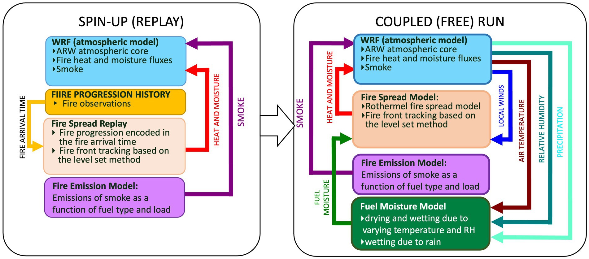
Figure 1. Schematic representation of the initial spin-up phase during which the fire progression history is replayed (left) and the fully coupled simulation (right).

This study utilizes the FireFlux II experiment, which provides a unique opportunity to evaluate simulated fire-induced circulation based on the in-situ observations of vertical velocities from sonic anemometers. Unfortunately, such data are not available for large wildfire events like the Creek Fire. Therefore, to assess the initialization methods in the Creek Fire wildfire case study, plume top height data are used as a proxy to assess if the model realistically resolved pyroconvection since the vertical velocity scale and the plume top height are closely related (Moisseeva and Stull, 2021).

The Methodology (Section 2) introduces fire initialization methods, outlines the modeling framework, and describes WRF-SFIRE model configurations used to quantify how tested fire initialization methods might impact fire growth and smoke forecasts. In the Results (Section 3), we present the findings from the sensitivity tests outlined in the methodology section. In (Section 4) we discuss the results and limitations of the presented methods in terms of operational applications. Finally, in the Conclusion (Section 5), we summarize key findings.

2 Methods

In order to assess the potential influence of different fire initialization methods on both fire growth and plume development within a coupled fire-atmosphere model, we developed and tested three methodologies. These methodologies, presented schematically in Figure 2, enable the initialization of the fire model’s state using perimeter observations. The analyzed methods included:

a. Instantaneous ignition of the whole fire area within the fire perimeter.

b. Instantaneous ignition along the fire perimeter with the fuel removed from the inside of the fire (simple method).

c. Gradual ignition from the fire history (spin-up method).

FIGURE 2

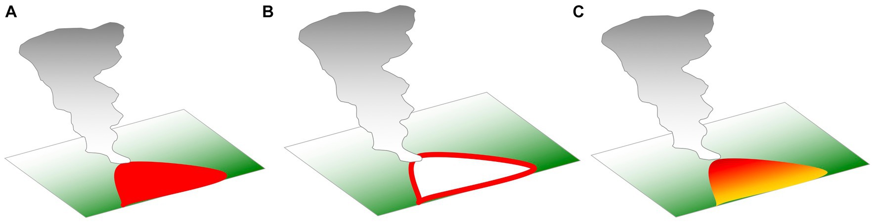
Figure 2. Schematic diagrams of three fire initialization methods investigated in this study: (A) Instantaneous ignition (red fill), (B) Simple initialization—ignition along the fire perimeter after removal of the fuel from the inside represented by the white fill, (C) Spin-up method with the gradient fill representing the gradual ignition during the fire replay period. The green shading represents unburned fuel.

In the first method, the entire perimeter and the fuel within the perimeter are ignited instantaneously (see Figure 2A). For this setup, the fire simultaneously consumes the fuel inside the fire and the fuel surrounding it as the fire propagates outward. Once the fuel within the burning region is consumed, a firefront forms and extends away from the burned area. Panel (b) in Figure 2 illustrates the second method, where the fire is ignited along the fire perimeter only. In this method, the fuel within the fire perimeter is removed before the ignition. Finally, panel (c) illustrates the method where fire growth prior to the initialization time is prescribed using an external fire arrival time. In this scenario, the fuels inside of the initial fire perimeter are burned at a time that is prescribed by the fire arrival time. Once the fire reaches the time that corresponds to the fire initialization time, the fire rate of spread model is turned on and the fire arrival time is no longer used to prescribe the fire growth. This method is a simplification of the original methods used by Kondratenko et al. (2011), Mandel et al. (2012), and Farguell Caus et al. (2018), which controls the ROS. Here we simply use a spatial interpolation to the fire model grid of the fire arrival time defined at the ignition point and two perimeters to prescribe the initial fire evolution. In this study, we used the data assimilation functionality included in WRF-SFIRE which enables initialization of the fire based on the fire arrival time as described in Mandel et al. (2014). It has to be noted that although the first two of these methods are less realistic than the other two, all of them would provide identical results when applied to uncoupled simulations. Therefore, in order to highlight the unique requirements of the coupled models all of them were tested on the experimental fire.

In the first step, we deployed all three methods to the simulation of the FireFlux II experimental fire and evaluated the model-resolved vertical velocities. Next, we applied two best-performing ones to a wildfire and assessed the vertical plume extent and fire growth.

2.1 Simulations of experimental fire (FireFlux II)

The initial investigation of the ignition procedures leveraged idealized WRF-SFIRE numerical simulations of a grassland fire on flat ground, mimicking the FireFlux II experimental burn. Our simulation configuration follows the one used to provide the forecasting support during the FireFlux II, which is outlined in Clements et al. (2019). The domain covered an area of 1000 × 1600 m (Figure 3) with a grid spacing of 10 m for the atmospheric grid and a fire mesh with 1 m grid spacing (1:10 refinement ratio). The model top was set to 1,200 m and 80 vertically stretched levels were used with depths varying from 2 m at the surface to 37.75 m at the domain top. Open boundary conditions were used so that the fire-induced updraft would not contaminate the inflow. The simulation was started at 15:00 UTC on January 31st^, 2013, and the model was run for 15 min with a time step of 0.25 s. The output was saved at 5 s intervals. The fire ignition was started at 15:04:12 (hh:mm:ss), in the form of two walking ignitions represented by yellow and orange lines in Figure 3. The burn plot was predominately covered with tall grass and had an overall fuel moisture content of 18%, a depth of 1.25 m, and a load of 1.08 kg m⁻¹. The model was initialized with a uniform fuel set within the burn plot to category 3 (Albini, 1976), and dead fuel moisture of 18%. The atmospheric model was initialized using vertical profiles of wind speed and direction, temperature, and moisture derived from a nearby tall tower and radiosonde observations before the burn.

FIGURE 3

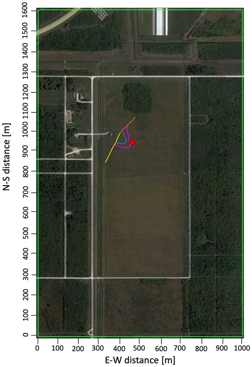
Figure 3. Model domain (green rectangle) with the location of ignition lines (yellow and orange), the measurement tower (red cross), and the perimeters at 15:05:00 and 15:05:12 s derived from IR observations (blue and magenta lines).

A total of three idealized simulations were analyzed. The benchmark simulation was started from the walking ignitions, and three additional simulations were performed with fire initialization procedures outlined in Figure 2. These initialization runs were executed as a continuation of the benchmark run. The restart file from the benchmark run was saved 4 min into the simulation (at 15:04 UTC). Then, three versions of this file were created by updating the fire arrival time according to the presented ignition methods. Each of the initialization cases was then executed starting from 15:04 UTC.

The instantaneous ignition from the fire area represented in Figure 2A, continued the benchmark simulation by restarting from the benchmark simulation at 15:04. Then the fire arrival time in the restart file was set to 15:05:12 (72 s since the beginning of the restart) everywhere within the second (purple) perimeter in Figure 3. The time of 72 s was selected so that the ignition ended before the fire reached the measurement tower. Starting from that point, the model continued in a fully coupled mode, allowing the fire to evolve from the shape forced by the fire arrival time used as the input.

The ignition from the fire perimeter with fuel masking, schematically shown in Figure 2B, was restarted with the fire arrival time set to 72 s after the simulation started, but only along the second (purple) perimeter presented in Figure 3. Starting from that point, the model continued in a fully coupled mode, allowing the fire to grow only outward of the ignited perimeter since the fuel inside of the fire perimeter was removed.

To implement the gradual ignition in the spin-up method, shown schematically in Figure 2C, first, two fire perimeters were manually generated by outlining the fire contour based on the infrared camera footage at 15:05:00 and 15:05:12. These perimeters correspond to 60 s, and 72 s from the simulation restart time. The fire arrival time used to drive the initial fire progression history was generated using a bi-harmonic spline interpolation of the 2D time arrival data including the time of the ignition which was 12 s since the simulation start, and the two observed fire perimeters shown in Figure 4 (60 s and 72 s). The resulting fire arrival time presented in Figure 4 was used to prescribe the initial fire propagation and the release of the heat and moisture fluxes from the fire into the atmosphere. This gradual ignition phase covered the initial fire evolution between the ignition time (15:04:12) and the time of the second perimeter (15:05:12). This spin-up phase corresponds to the period between 12 s and 72 s from the beginning of the simulation, during which the fire model is forced to replay the fire history as shown in the left panel of Figure 1. After the fire replay, the fire model continued to forecast the fire in a fully coupled mode as shown schematically in the right panel of Figure 1.

FIGURE 4

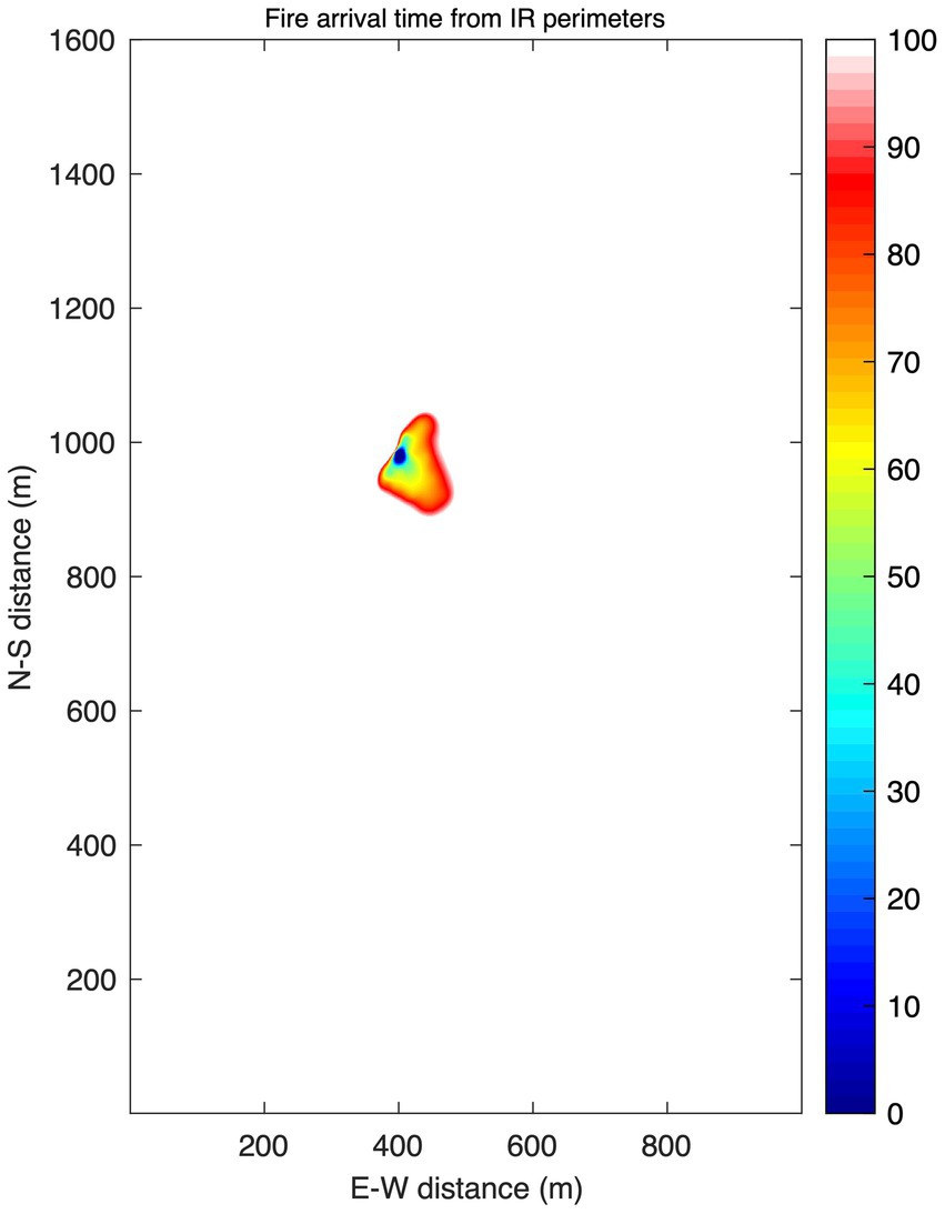
Figure 4. Fire arrival time (s) representing the history of the fire propagation used in the gradual ignition case, derived from the ignition origin at 15:04:12, as well as the fire perimeters at 15:05:00 and 15:05:12 presented in Figure 3.

2.2 Wildfire simulations (Creek Fire)

Since the first fire initialization method (instantaneous ignition) did not provide realistic results for the idealized FireFlux II simulation (see Section 3 below), only the last two fire initialization methods were tested in the wildfire case: the simple instantaneous perimeter ignition with fuel masking and the gradual ignition from the fire history during the spin-up. Both methods were applied to the Creek Fire, which started southwest of Big Creek, CA on September 4th, 2020, and burned a total of 379,895 acres between Fresno and Madera counties.

In the FireFlux II case study described previously, the performance and viability of different fire initialization methods were analyzed by comparing simulated fire-induced vertical velocities to in-situ observations. Unfortunately, in-situ observations of fire-induced vertical velocities are generally not available for wildfire events. Therefore, in order to analyze initialization methods at a larger scale of a wildfire, it is necessary to determine a proxy to fire-induced vertical velocity that would be available from observations. It is well established that the dynamics of fire-induced smoke plumes, and their height of injection into the atmosphere, are driven by ambient conditions and the wildland fire’s energy release (Kahn et al., 2008). More precisely, the dynamics of plumes are influenced by several key factors, including the buoyancy flux resulting from convective heat generated by fires in the combustion zone, and the release of latent heat through water vapor condensation within the plume (Freitas et al., 2007). Since fire-induced updrafts, plume rise, and therefore subsequently plume height, are driven by similar dynamics, satellite-derived plume height can be used as a proxy of fire-induced vertical circulation for the analysis of initialization method performance when simulating a real wildland fire case. Moisseeva and Stull (2021) used WRF-SFIRE in idealized large-eddy simulation (LES) mode to develop a simple parameterization of the mean plume rise as a function of the vertical velocity scale. They found that crosswind integrated smoke injection height for a fire of any shape and size can be modeled with a simple energy balance because there exists a linear dimensionless relationship between updraft velocity scales and plume vertical penetration distance. They used experimental burn data to constrain and evaluate their study starting at a small scale, and then evaluating at a larger scale with the RxCADRE burn data (RxCADRE 2012).

Based on a similar concept, in this study, we used an experimental burn with in-situ observations of vertical velocities to investigate the initialization methods at small scales, and then we used plume top height as a proxy for vertical velocities associated with pyroconvection during a wildfire without in-situ observations. Each model simulation that used a different fire ignition strategy was evaluated using plume top heights above sea level (ASL) derived from the Multi-angle Imaging Spectroradiometer (MISR; Kahn et al., 2008). Based on the availability of MISR overpasses 3 days were selected for the analysis: September 20th, 27th, and 29th of 2020. The plume top height in the simulation was estimated using the passive tracer corresponding to PM_2.5. The threshold of 1 μg m⁻³ was used to determine the vertical plume extent, which is similar to the threshold used by Kochanski et al. (2021). Additional information about MISR data, as well as details about the data processing are presented in the Supplementary material.

As in the FireFlux II case study, we first executed a benchmark simulation, which ran continuously from September 5th to the 29th of 2020. In this simulation, the fire evolution derived from satellite data as well as airborne infrared observations was used to constrain the fire progression in the simulation using the SVM method implemented by Farguell et al. (2021). Unlike the forecast runs, this simulation was executed continuously from start to finish. This simulation is considered a benchmark, since it is based on best-guess fire progression (according to remote sensing observations) and therefore represents the best possible realization of the fire and smoke dynamics. More details about the SVM method and the fire arrival time derived using this method are presented in Supplementary Figure S1.

The atmospheric component of WRF-SFIRE was initialized with the Climate Forecast System Reanalysis (CFSR 6-hourly) dataset (Saha et al., 2014). WRF was configured with three nested domains, D01, D02, and D03, as seen in Table 1. The fire mesh within the innermost domain D03 had a grid spacing of 27 m.

TABLE 1

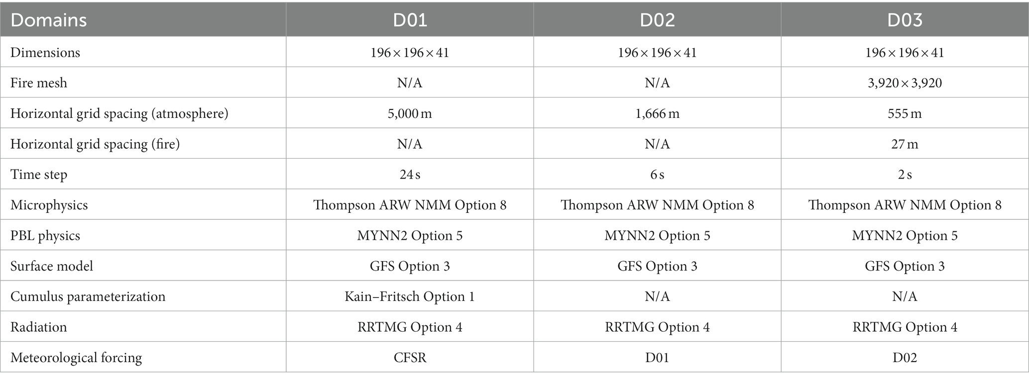
Table 1. WRF-SFIRE configuration for the real case.

For each day in the study period, two fire-atmosphere forecast initialization methods were tested. The first simulation used the simple method with instantaneous ignition (Figure 2B), while the second simulation used the spin-up method with gradual fire ignition illustrated in Figure 2C. The initialization with the simple method was performed based on the most recent fire perimeter taken from the National Infrared Operations (NIROPS) data, which were available prior to the forecast start time (see Figure 5A). The most recent perimeter (black line) is used to ignite the fire (see yellow line in Figure 5A), while unburnable fuel (gray fill) is set inside of it.

FIGURE 5

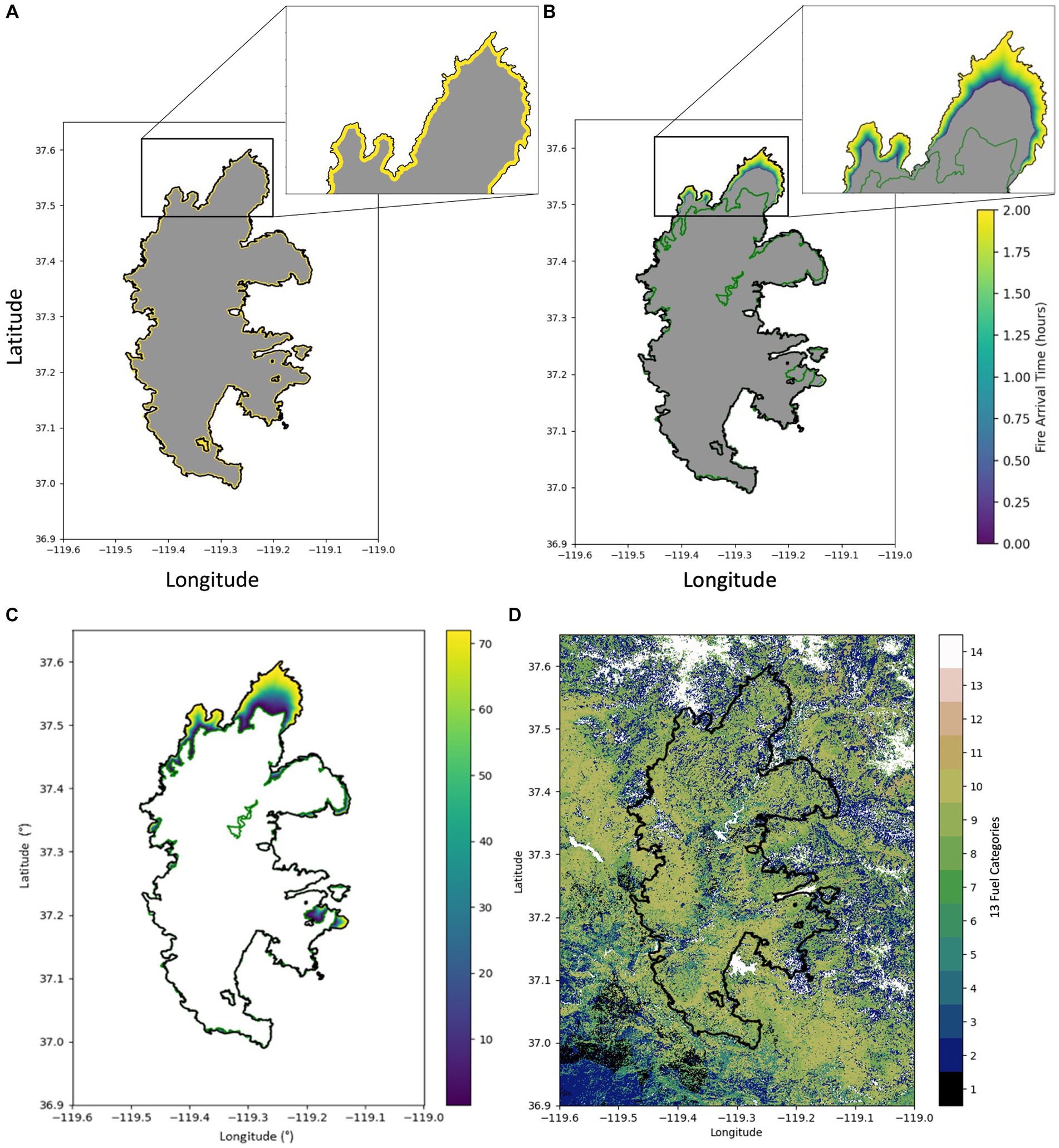
Figure 5. (A) Fire ignition of the simple initialization method. The perimeter ignition represented by the yellow line is based solely on the most recent perimeter, the gray fill (masking) represents fuel removed from the inside of it. (B) Initialization of the gradual ignition in the spin-up method. (C) The fire arrival time estimated based on two consecutive perimeters used to control the gradual ignition. (D) The Landfire fuel map used in the simulations showing distribution of 13 Albini (1976) fuel categories.

The spin-up initialization method with gradual ignition leveraged two perimeters as shown in Figure 5B. The fire history generated by interpolating the fire arrival time between two perimeters (presented in Figure 5C) was used to perform the gradual ignition within the spin-up method. Figure 5 presents an example for 09/20, but the same method was used also for 09/27 and 09/29. The timing of the perimeters used for the periodic initialization for all analyzed days is presented in Table 2. The ignition maps used for all the days are presented in Supplementary Figures S2, S3.

TABLE 2

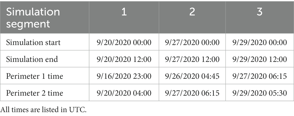
Table 2. Timing of the simulations and the IR perimeters.

To identify areas of active growth (indicated by the yellow fill in Figure 5B), for each run, the inside of the prior perimeter was masked out to represent already burned fuel. The masking (fuel removal) was performed with an extra margin extending outside of the first perimeter. This buffer deactivated ignition over the sections of the fire perimeter where subsequent perimeters overlapped, or were closer together than the buffer size, indicating no active fire propagation. The removal of fuel during the masking phase has a dual purpose. It allows for the deactivation of fire over the regions of marginal or no fire activity and to prevent fire from propagation inward from the fire perimeter. Even where the perimeters are overlapping, the fire arrival time forces the fire model to start the fire. However, the mask, which removes burnable fuel, effectively stops the fire propagation by setting the rate of spread to zero at these locations. Consequently, the fire is gradually ignited only in the regions of actively propagating fire, indicated by the gradual fill color in Figure 5B, following the reconstructed fire progression shown in Figure 5C, whereas the instantaneous ignition ignites fire everywhere around the entire perimeter whether there is known fire activity there or not as shown in Figure 5A. The method introduced here builds upon a more straightforward approach employed by Herr et al. (2020). Herr et al. (2020) utilized fire replay, similar to our approach, but without the incorporation of selective ignition through masking. In their study, the fire was ignited uniformly across the entire second perimeter.

3 Results

3.1 Experimental fire (FireFlux II)

The time series of the updraft velocities near the fire front simulated in the benchmark run (started from two ignition lines corresponding to the actual FireFlux II ignition procedure and ran continuously for 15 min) are shown in Figure 6A. The signature of pyroconvection was visible first at 20 m above the ground level (AGL) and, then subsequently at 10 m and 6 m, as the tilted plume impacted the sensors at lower elevations. The maximum simulated updraft velocities were equal to 5.2 m s⁻¹, 4.4 m s⁻¹, and 3.5 m s⁻¹ at 20 m, 10 m, and 6 m AGL respectively, compared to observed updraft velocities of 7.5 m s⁻¹ 5.2 m s⁻¹, and 4.2 m s⁻¹ (see Figures 6A,D respectively). The main reason for the discrepancies between the simulated and observed updraft velocities is that the simulated fire head slightly missed the tower location. We hypothesize that it was due to a wind direction shift that occurred after the ignition and could not be accounted for in idealized simulations with open boundary conditions. The maximum simulated updrafts at the fire head were significantly higher and closer to observations.

FIGURE 6

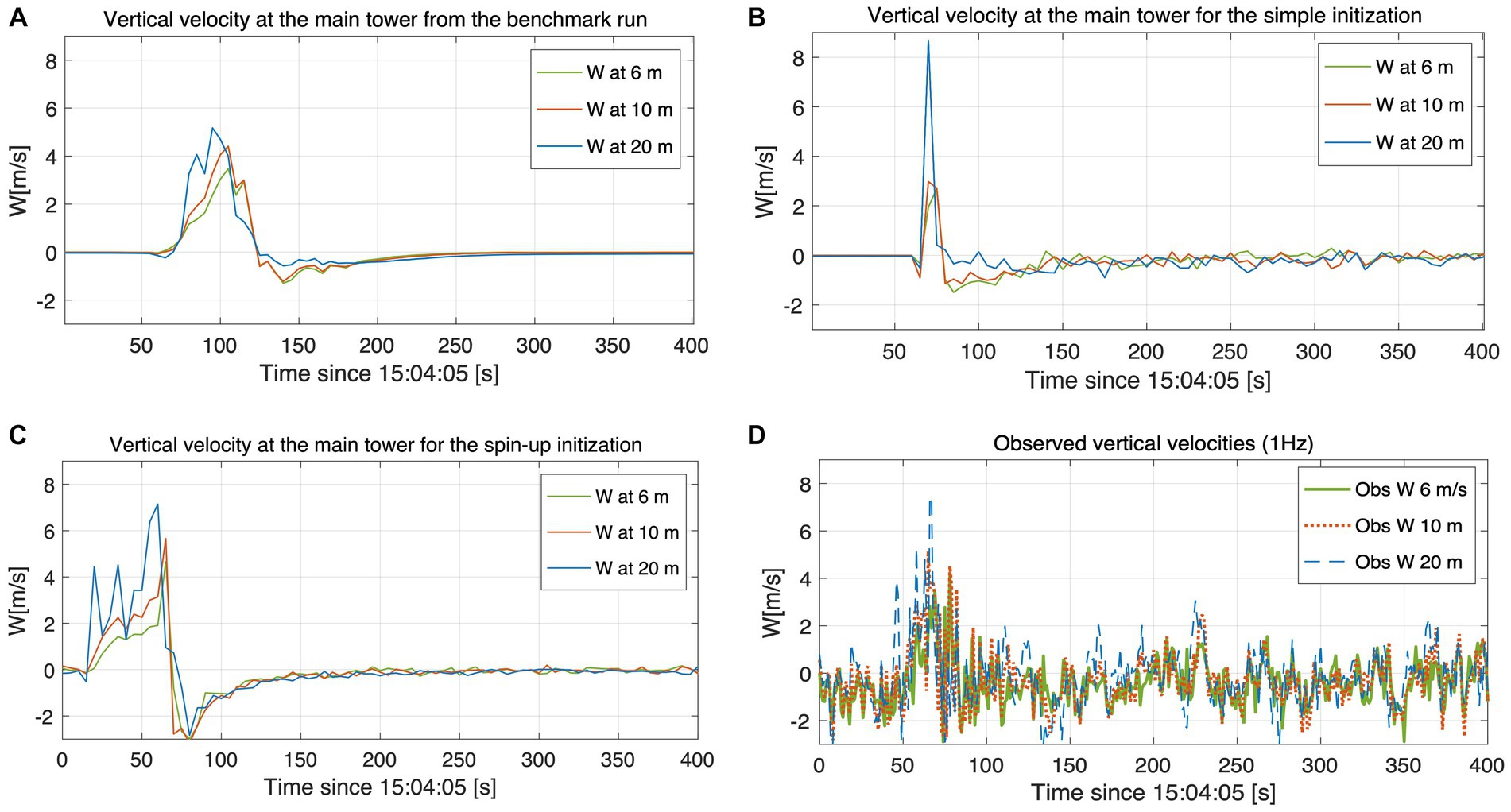
Figure 6. Simulated updraft velocities at the main tower at 6 m, 10 m and 20 m above the ground level from (A) the benchmark run, (B) instantaneous ignition with fuel removal, (C) gradual ignition (spin-up), (D) observed vertical velocities at 1 Hz.

3.1.1 Instantaneous ignition from the fire area

As a first test, the fire was instantaneously ignited from the fire area encompassed by the fire perimeter at 15:05:12 presented as the purple line in Figure 3. This simulation led to an unrealistically high fire heat flux that induced very strong updraft/downdraft couplets that numerically destabilized the model. The fire did not even reach the location of the tower, as the updraft velocities at 10 m reached values of 52 m s⁻¹, making the atmospheric component of the model numerically unstable due to a violation of the vertical Courant–Friedrichs–Lewy (CFL) condition.

3.1.2 Ignition from the fire perimeter with no inside fuel

In the second test, the same fire was instantaneously ignited, but only along the fire perimeter. In this case, the fuel inside of the fire perimeter was set to fuel category 14 (no-fuel), so that the fire could propagate only outward from the initial perimeter. By removing the fuel from inside the perimeter, the formation of the secondary fire front behind the fire head was avoided. The updraft structure from this WRF-SFIRE simulation resembles the benchmark simulation (see Figure 6B). The vertical velocities were increasing with height as expected, but their maximum values at 6 m and 10 m AGL were significantly smaller than in the benchmark run (2.7 m s⁻¹ and 3.0 m s⁻¹ vs. 3.4 m s⁻¹ and 4.4 m s⁻¹), while the maximum updraft at 20 m was much stronger than in the benchmark run (8.6 m s⁻¹ vs. 5.2 m s⁻¹). These discrepancies suggest that as the simulated fire passed the tower location, the fire-atmosphere interaction wasn’t well established, and the heat abruptly injected into the atmosphere during the ignition caused puff-like plume behavior where the updraft was over and underestimated at higher and lower levels, respectively.

3.1.3 Gradual ignition from the fire replay

The last fire initialization method shown in Figure 2C leveraged the fire replay functionality schematically represented in the left part of Figure 1. The time series of the vertical velocities simulated using the spin-up method shown in Figure 6C suggest that at the restart time, the fire plume was fully evolved. The maximum updraft velocities of 7.1 m s⁻¹, 5.6 m, and 4.6 m s⁻¹ at 20 m, 10 m, and 6 m, respectively, better resembled the observations and benchmark simulations relative to the other perimeter ignition methods.

The updraft velocities increased with height and the time was shifted by 5 s between the peaks suggesting that the plume was tilting downwind. There were no stability issues in this run, as the fire was not ignited instantaneously. The replay from the fire history ensured that the fuel got depleted within the fire perimeter, so the formation of an artificial secondary fire front was prevented. Since the fire is ignited gradually from the fire history, the atmosphere equilibrates with the fire during the fire replay procedure, which results in significantly improved fire plume representation at the start of the simulation relative to the other methods tested in this study.

3.2 Wildfire case (Creek Fire)

Two ignition procedures were tested on the wildfire event. The first fire initialization method tested was the simple method (instantaneous ignition along the perimeter with the fuel removed from its inside). The second fire initialization method tested was the spin-up method with gradual ignition. In the latter case, the fire was gradually ignited only in the regions of actively propagating fire, indicated by a gradual fill color in Figure 5B, whereas in the former case, the instantaneous ignition activated fire everywhere around the entire perimeter whether there was known fire activity there or not (yellow fill in Figure 5A). For each ignition procedure, we evaluated the overall fire growth and the vertical plume extent.

As shown in Figure 7 and Supplementary Table S3, the fire initialization method can have a significant impact on the simulated fire progression. Figure 7 represents the first 12 h of fire growth for each fire initialization method and simulation segment. Supplementary Table S3 in the Supplementary material shows total fire growth in acres for the same period and their percentage error compared to linearly interpolated IR fire perimeter observations. The simulation that utilizes the simple method (red line) during initialization experienced much more rapid growth relative to the simulation initialized using the spin-up method (dotted blue line). The fire growth in the simulations initialized with the simple method was significantly overestimated when compared to the estimate based on the observations represented by the dashed black line. During the first day, the simulation with the simple method overestimated the fire growth by around 3,800 acres while the one with the spin-up method reduced this error by a factor of three to around 1,300 acres. On September 27th, the difference between the methods was even greater. Here the simple method overestimated the fire growth by approximately 6,500 acres, while the spin-up ignition method reduced this error to 400 acres (almost 16 times). During the last analyzed day (September 29th) the spin-up method underestimated the fire growth by 200 acres, while the simple method overestimated the fire growth by around 8,000 acres. In summary, the spin-up method reduced the fire growth absolute percentage error compared to observations from 273 to 94% for the first day, from 484 to 29% for the second day, and from 791 to 21% for the last day. These results indicate that the spin-up method results in a better representation of the fire growth as compared to the simple method. It has to be noted though, that this improvement is partially due to the selective ignition and masking procedure being a part of the spin-up method. The selective ignition requires two consecutive perimeters to identify the fire growth and therefore, it cannot be done based on a single perimeter, which is what is utilized during initialization with the simple method.

FIGURE 7

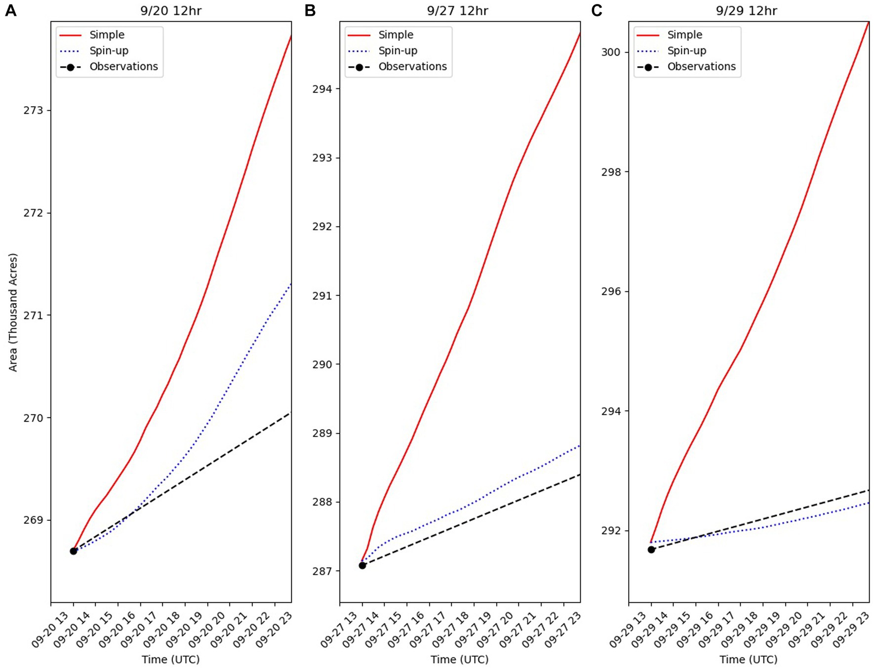
Figure 7. Comparison of fire growth for the first 12 h of the forecast between instantaneous ignition (simple method)—solid red, and gradual ignition with the fire replay (spin-up method)—dotted blue, for (A) September 20th (B) 27th, and (C) 29th of 2020. The black dots represent the fire area derived from the infrared perimeter data. The black dashed lines (observations) are the linear interpolation between consecutive infrared fire perimeters.

To assess the impact of the initialization procedure on model’s ability to resolve pyroconvection, the vertical plume extent from the simulations was compared to MISR observations for September 20^th, 27^th, and 29^th. Details about the MISR processing as well as the MISR error estimate are presented in the Supplementary material. Supplementary Tables S1, S2 included herein, list overpasses used in the study and provide statistics of the simulated plume top heights. Figure 8 presents the box and whisker as well as violin plots for the analyzed days. The red line presented there shows the median MISR-derived plume height, while the red shading represents the estimated plume height retrieval error of ±260 m. As shown there, the simulations initialized with the simple method produced higher plume tops than the spin-up method or the benchmark for all days. It is important to mention that the benchmark run can be treated as a predictability limit for WRF-SFIRE, which in this case is constrained by the observed fire progression. For that reason, it can serve as a reference point during the discussion of the results from the tests of the initialization methods.

FIGURE 8

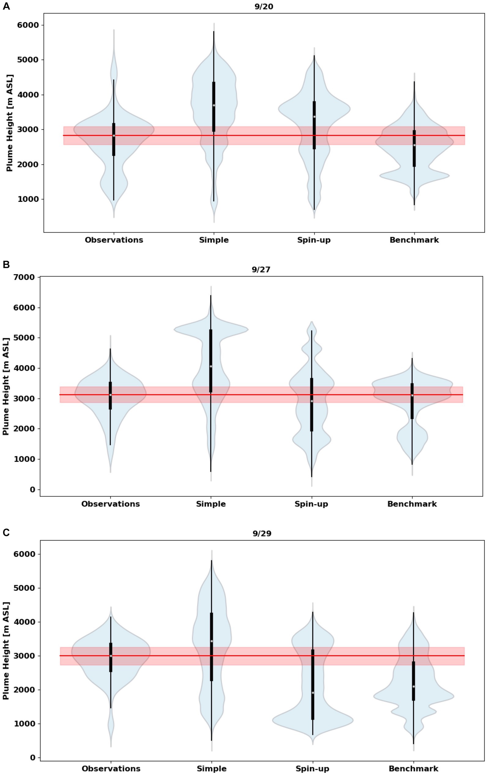
Figure 8. Box and whisker plots overlaid with the violin plots comparing between the observed (MISR) and WRF-SFIRE simulated plume top heights from the benchmark simulation and two fire initialization methods—instantaneous ignition (simple) and gradual ignition (spin-up) for: September 20th (A), 27th (B), and 29th (C) of 2020. The red line represents median observed plume height and the red shading represents uncertainty in the MISR plume top height retrieval estimated to be around 260 m (see the Supplementary material).

For all days it can be observed that the maximum plume top heights from the simulations initialized with the spin-up method were closer to the benchmark simulation than the simulations initialized with the simple method. During the 09/20 simulations, even though on average the spin-up method overestimated the plume heights, it was closer to the observations than the simple method. The violin plot for 09/20 indicates that the spatial distribution of plume top heights shown in violin plots was captured well in the benchmark simulation. The simulation with the spin-up method rendered the maximum plume top heights of (5,109 m ASL), which compared favorably to the MISR observations of plume top heights (5,523 m ASL). While the simple method (instantaneous ignition) simulation had a maximum plume top height that was in relatively good agreement with MISR observations (5,806 m vs. 5,523 m ASL), there were significant mismatches in the distribution of plume tops as seen in the violin plot indicating an unrealistically large number of plume tops exceeding 4,000 m ASL. It has to be noted that although the simulation initialized with the spin-up method shows a higher concentration of points above 3,500 m ASL compared to MISR, the violin plot in Figure 8A shows a similar pattern of two peaks of smoke height, making the simulation initialized with the spin-up method closer to the observations than the simulation initialized with the simple method. To further investigate the simulated pyroconvection, we also generated spatial plume top height maps based on the model output at the time closest to the MISR overpass (see Figure 9 and Supplementary Table S1).

FIGURE 9

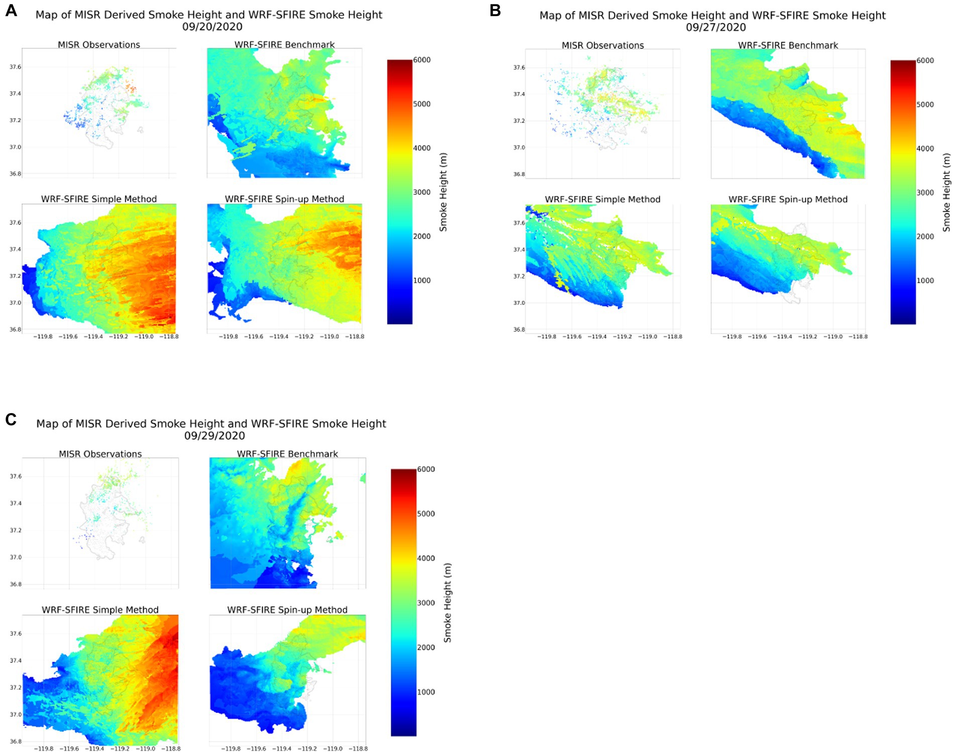
Figure 9. Maps of smoke height from MISR (m ASL), the benchmark simulation, the spin-up method (gradual ignition) simulation, and the simple method (instantaneous ignition) simulation for: September 20th (A), 27th (B), and 29th (C) of 2020.

The spatial maps show time snapshots of the vertical plume extent from simulations and observations and are intended to provide more insight into the differences between the analyzed cases. It must be noted that only a fraction of plumes is effectively used for the retrieval of the plume top heights by MISR. Therefore, the white spaces in observation panels should be treated as missing data rather than areas without smoke.

As can be observed in Figure 9A, on September 20th MISR indicated that the highest smoke layer was located on the northeastern flank of the fire while the lowest heights were to the southwest. The overestimation of the plume top heights as well as the extensive area of elevated smoke in the eastern part of the domain in the case initialized with the simple method were the result of the instantaneous ignition of the entire fire perimeter. The fire heat fluxes from the simple ignition case were overestimated compared to the benchmark, which resulted in unrealistic updraft velocities, and therefore, an overestimated spatial extent of high plumes. The benchmark simulation provided a similar spatial distribution of the plume heights to the MISR estimates with the highest plumes near the north-east edge of the fire and lowest plumes in in the south-western region. The spin-up method produced a similar pattern but with a larger extent of the plumes above 4,000 m.

On September 27th, the benchmark simulation showed very good agreement with the observations, with the median plume height matching well the MISR data. The spin-up simulation on that day showed a slightly lower median plume height than the benchmark simulation and observations, but within the estimated error of the MISR data, indicated in Figure 8 by the red shading. As shown in Figure 8B, the initialization with the simple method again had the highest median smoke height out of all the simulations and, in a statistical sense, performed worse than the benchmark and spin-up runs when compared to the statistics of the observed heights. It has to be noted that on September 27th there was a residual upper layer of smoke entering the fire domain from domain 2, which was removed from the plots to show the extent of the primary smoke associated with the fire activity.

On September 29th, the simple method simulation yielded the highest smoke layer. Nevertheless, it’s noteworthy that on this particular day, both the benchmark and the spin-up simulation tended to underestimate plume heights. Consequently, the simple initialization method demonstrated a closer alignment with observed data on a statistical basis. The accompanying violin plots in Figure 8C, along with the plume top height map in Figure 9C however, illustrate the prevalence of plume height discrepancies, with a substantial interplay between overestimations and underestimations that tended to balance each other out. MISR observations show the highest vertical plume extent along the northern flank of the fire which is also seen in the benchmark and spin-up method simulations. However, the simple method simulation overestimated the plume top heights across the fire as well as east from it, where the overestimation is most evident. The simple method simulation was the only simulation that significantly overestimated the maximum plume top heights on that day. This method produced much higher smoke columns (5,803 m ASL) compared to the spin-up (4,278 m ASL), the benchmark simulation (4,258 m ASL), and the MISR observations (4,138 m ASL). Compared to MISR observations, the spin-up method case was within ~100 m of the highest observed smoke height, whereas the simple method case had smoke heights ~1,700 m higher than observations, which indicates a much better performance of the spin-up method initialization than the simple one.

4 Discussion

The presented work focuses on methods for integrating fire perimeters into a fire-atmosphere model through cyclic initialization. It evaluates various approaches for initializing fires within the model and examines their impact on fire growth and plume rise forecasts using experimental burns and wildfires. Numerical simulations for the experimental burn and a wildfire case indicate that fire spread and plume rise forecasts were sensitive to the fire initialization method. In the case of the experimental burn (FireFlux II) simulations, the spin-up method better represented plume dynamics relative to the other fire initialization methods. The simulated vertical velocities in the gradual ignition case were closer to the observations relative to the other simulations. The vertical winds matched well the observations increasing from 4.6 m s⁻¹ at 6 m to 7.1 m s⁻¹ at 20 m compared to the measured values of 4.2 m s⁻¹ at 6 m and 7.5 m s⁻¹ at 20 m. Of the three approaches evaluated here, the two best-performing fire initialization methods (spin-up or gradual ignition and simple or instantaneous ignition with fuel removal from the inside of the perimeter) were applied to a wildfire case. For each of these aforementioned fire initialization methods, fire growth and vertical plume extent were evaluated with MISR plume top heights on three different days of the Creek Fire. For the wildfire case study, the simulation that used the simple method generally overestimated fire growth and vertical plume extent relative to the benchmark simulation and observations. The simulation that used the spin-up technique improved both the vertical plume extent as well as the fire growth. The error in the fire growth in the spin-up (gradual ignition) case was 3 to 35 times smaller than in the simple (instantaneous ignition) case. It must however be noted, that this improvement is due to both the gradual ignition as well as the masking procedure enabling selective ignitions within the spin-up method. However, selective ignition requires two consecutive perimeters to identify the historical fire growth and therefore, it cannot be performed based on a single perimeter as used in the simple (instantaneous ignition) method. For that reason, the simple initialization method cannot take advantage of the selective ignition utilized in the spin-up method.

In the wildfire test case, analyzed using MISR data, the error in predicted vertical plume extent was reduced by half for the spin-up method when compared to the simple method (11 vs. 5%). The horizontal extent of high-level smoke was significantly overestimated in the simple initialization case while using the spin-up initialization method, utilizing selective fire ignition, resulted in a more realistic plume structure when compared to the benchmark simulation.

It should be emphasized that the spin-up method outlined in this work requires two IR fire perimeters as a source of data for fire reconstruction needed for the fire spin-up phase and for the identification of the actively burning regions. The reliance on IR fire perimeters introduces numerous limitations to the initialization method. Operational IR perimeters are not globally available, which makes this method usable only for countries with established airborne fire mapping programs. Even in the US, infrared perimeters are available only for selected fire incidents, and typically perimeters are not available at the very beginning of the fire.

It also must be noted, that in our analysis, perimeters collected after the fire incident were used. The fire progression history was replayed to the time corresponding to the end of the spin-up phase which was set to 2 h. This represents the best possible scenario when the perimeter data are available at the time of the forecast start +2 h. However, even in cases of fire events with airborne observational support, IR perimeters often aren’t available in real-time and may experience multi-hour latency before they become publicly available and ready for assimilation. For example, the IR perimeters posted by the National Infrared Observations (NIROPS) in the morning typically reflect the fire extent mapped the previous night, which means that at the time when these perimeters become available, they are often outdated. In such cases, the forecast would need to be started either way earlier, so that the end of the spin-up corresponds to the time of the IR data retrieval, or the fire progression between the time of the overflight and the forecast would need to be ignored. For many fires experiencing marginal nighttime activity, it could be acceptable but for fire events remaining active at night, this assumption could introduce significant errors due to inaccurate representation of the state of the fire at the start of the forecast.

To reduce the issues associated with this delay, one could incorporate satellite observations. The recent advances in satellite data processing and fire spread reconstruction open new possibilities in the context of fire initialization using presented methods. Although tested on the IR airborne perimeters the methodology presented in this study could be also used to leverage perimeters obtained based on satellite data. For example, the method presented by Chen et al. (2022) that allows the creation of twice-daily fire perimeters based on the VIIRS data could serve as a source of synthetic fire perimeters for the presented initialization method. Additionally, machine learning techniques like SVM, could be used to reconstruct fire progression history and provide fire perimeters at arbitrary times. However, the usability of the satellite data will still depend on the data latency and will require postprocessing methods converting satellite rasters to synthetic perimeters. The latency of satellite data (up to 4 h for VIIRS) although lower than the airborne observations is still significant and will limit the accuracy of the representation of the fire state at the beginning of a forecast or will require starting the forecast hours earlier to sync the time of the end of the spin-up phase with the time of the satellite overpass. The fire tracing methods leveraging geostationary satellites like the one proposed by Liu et al. (2023) could address this problem by providing synthetic fire perimeters at hourly intervals. However, the coarse resolution of the underlying GOES data (~2 km) may limit the applicability of such methods to large and fast-propagating fires. Considering the limitations of satellite fire detections, a dedicated airborne fire mapping program providing on-demand high-resolution perimeters with low latency is expected to provide the best results in operational forecasting using the proposed spin-up method outlined in this work.

It must be noted that the forecast spin-up effectively increases the length of each forecast. The extra 2 h of the forecast spin-up would mean increasing the computational time by about 17% in the case of a 12-h forecast. For a typical forecast length of 24 or 48 h, this increase would be reduced to 8% or 4%, respectively.

5 Conclusion

Various initialization methods have been tested on the experimental fire (FireFlux 2) and wildfire test case (Creek Fire). The experimental fire provided unique in-situ data that enabled the examination of in-plume vertical velocities to assess the impact of the initialization method on the model’s ability to resolve fire-induced circulation at the beginning of a simulation of an ongoing fire. In the wildfire case, the fire growth and the plume top height estimates from MISR were used for initialization method assessment. The improvements in the representation of the fire-induced updrafts, vertical smoke extent, as well as fire growth, suggest that the spin-up method is the optimal fire initialization strategy when running a coupled fire-atmosphere model like WRF-SFIRE for ongoing fires. Since accurately forecasting wildfire plume rise is especially important for correctly predicting the downwind transport of wildfire smoke, which can be sensitive to the plume injection height (Mallia et al., 2018, 2020a; Kochanski et al., 2021), this method would also likely be beneficial for smoke forecasting applications and modeling frameworks.

Data availability statement

The numerical model used in this study is available at https://github.com/openwfm/WRF-SFIRE. The WRFx system used for data processing is available at: https://github.com/openwfm/wrfxpy. The raw data supporting the conclusions of this article will be made available by the authors, without undue reservation.

Author contributions

AK designed the study and methodology, generated the model simulations and data analysis, and prepared the manuscript. KC processed MISR data, analysed the Creek fire test case and helped prepare the manuscript. DM implemented the prototype of the wildfire initialization method and reviewed the manuscript. AF assisted with the data analysis and plotting, led the development of the fire initialization code in the WRFx system, and reviewed the manuscript. JM is the lead developer of the WRF-SFIRE code base, helped design the method, and reviewed the manuscript. KH assisted with data analysis and with the review of the manuscript. All authors contributed to the article and approved the submitted version.

Funding

This work was funded by NASA grants 80NSSC19K1091, 80NSSC22K1717, and 80NSSC22K1405, NSF grants DEB-2039552 and IUCRC-2113931, and CALFIRE grant 8GG21829.

Acknowledgments

The authors would like to acknowledge high-performance computing support from Cheyenne (doi: https://doi.org/10.5065/D6RX99HX) provided by NCAR’s Computational and Information Systems Laboratory, sponsored by the National Science Foundation. The authors are also grateful to the SJSU Fire HPC Support group for providing the computational assistance needed to carry out the model analyses shown here. The support and resources from the Center for High-Performance Computing at the University of Utah are gratefully acknowledged. This work also used the computing resources at the Center for Computational Mathematics, University of Colorado Denver, supported by the National Science Foundation award OAC-2019089.

Conflict of interest

The authors declare that the research was conducted in the absence of any commercial or financial relationships that could be construed as a potential conflict of interest.

Publisher’s note

All claims expressed in this article are solely those of the authors and do not necessarily represent those of their affiliated organizations, or those of the publisher, the editors and the reviewers. Any product that may be evaluated in this article, or claim that may be made by its manufacturer, is not guaranteed or endorsed by the publisher.

Supplementary material

The Supplementary material for this article can be found online at: https://www.frontiersin.org/articles/10.3389/ffgc.2023.1203578/full#supplementary-material

References

Albini, F. A. (1976). “Estimating wildfire behavior and effects” in General technical report INT-30 (U. S. Forest Service) Available at: http://www.treesearch.fs.fed.us/pubs/29574

Google Scholar

Andrews, P. L. (2013). Current status and future needs of the BehavePlus fire modeling system. Int. J. Wildland Fire 23, 21–33. doi: 10.1071/WF12167

CrossRef Full Text | Google Scholar

Banta, R. M., Olivier, L. D., Holloway, E. T., Kropfli, R. A., Bartram, B. W., Cupp, R. E., et al. (1992). Smoke-column observations from two forest fires using Doppler lidar and Doppler radar. J. Appl. Meteorol. 31, 1328–1349. doi: 10.1175/1520-0450(1992)031<1328:SCOFTF>2.0.CO;2

CrossRef Full Text | Google Scholar

Benik, J. T., Farguell, A., Mirocha, J. D., Clements, C. B., and Kochanski, A. K. (2023). Analysis of fire-induced circulations during the FireFlux2 experiment. Fire 6:332. doi: 10.3390/fire6090332

CrossRef Full Text | Google Scholar

Chen, Y., Hantson, S., Andela, N., Coffield, S. R., Graff, C. A., Morton, D. C., et al. (2022). California wildfire spread derived using VIIRS satellite observations and an object-based tracking system. Sci. Data 9:249. doi: 10.1038/s41597-022-01343-0

PubMed Abstract | CrossRef Full Text | Google Scholar

Clark, T. L., Jenkins, M. A., Coen, J., and Packham, D. (1996). A coupled atmosphere-fire model: convective feedback on fire-line dynamics. J. Appl. Meteorol. 35, 875–901. doi: 10.1175/1520-0450(1996)035<0875:ACAMCF>2.0.CO;2

CrossRef Full Text | Google Scholar

Clements, C. B., Kochanski, A. K., Seto, D., Davis, B., Camacho, C., Lareau, N. P., et al. (2019). The FireFlux II experiment: a model-guided field experiment to improve understanding of fire-atmosphere interactions and fire spread. Int. J. Wildland Fire 28, 308–326. doi: 10.1071/WF18089

CrossRef Full Text | Google Scholar

Clements, C. B., Perna, R., Jang, M., Lee, D., Patel, M., Street, S., et al. (2007). Observing the dynamics of wildland grass fires: Fireflux—a field validation experiment. Bull. Am. Meteorol. Soc. 88, 1369–1382. doi: 10.1175/BAMS-88-9-1369

CrossRef Full Text | Google Scholar

Coen, J. L., and Schroeder, W. (2013). Use of spatially refined satellite remote sensing fire detection data to initialize and evaluate coupled weather-wildfire growth model simulations. Geophys. Res. Lett. 40, 5536–5541. doi: 10.1002/2013GL057868

CrossRef Full Text | Google Scholar

Farguell Caus, A., Haley, J., Kochanski, A. K., Cortés Fité, A., and Mandel, J. (2018). Assimilation of fire perimeters and satellite detections by minimization of the residual in a fire spread model. Lect. Notes Comput. Sci 10861, 711–723. doi: 10.1007/978-3-319-93701-456

CrossRef Full Text | Google Scholar

Farguell, A., Mandel, J., Haley, J., Mallia, D. V., Kochanski, A., and Hilburn, K. (2021). Machine learning estimation of fire arrival time from level-2 active fires satellite data. Remote Sens. 13:2203. doi: 10.3390/rs13112203

CrossRef Full Text | Google Scholar

Freitas, S. R. K. M., Longo, R., Chatfield, D., Latham, M. A. F. S., Dias, M. O., Andreae, E., et al. (2007). Including the sub-grid scale plume rise of vegetation fires in low resolution atmospheric transport models. Atmos. Chem. Phys. 7, 3385–3398.

Google Scholar

Herr, V., Kochanski, A., Miller, V., McCrea, R., O’Brien, D., and Mandel, J. (2020). A method for estimating the socioeconomic impact of earth observations in wildland fire suppression decisions. Int. J. Wildland Fire 29, 282–293. doi: 10.1071/WF18237

CrossRef Full Text | Google Scholar

Kahn, R. A., Chen, Y., Nelson, D. L., Leung, F.-Y., Li, Q., Diner, D. J., et al. (2008). Wildfire smoke injection heights: two perspectives from space. Geophys. Res. Lett. 35. doi: 10.1029/2007GL032165

CrossRef Full Text | Google Scholar

Kochanski, A. K., Herron-Thorpe, F., Mallia, D. V., Mandel, J., and Vaughan, J. K. (2021). Integration of a coupled fire-atmosphere model into a regional air quality forecasting system for wildfire events. Front. For. Glob. Change 4:728726. doi: 10.3389/ffgc.2021.728726

CrossRef Full Text | Google Scholar

Kochanski, A. K., Jenkins, M. A., Yedinak, K., Mandel, J., Beezley, J., and Lamb, B. (2016). Toward an integrated system for fire, smoke, and air quality simulations. Int. J. Wildland Fire 25, 534–546. doi: 10.1071/WF14074

CrossRef Full Text | Google Scholar

Kochanski, A. K., Mallia, D. V., Fearon, M. G., Mandel, J., Souri, A. H., and Brown, T. (2019). Modeling wildfire smoke feedback mechanisms using a coupled fire-atmosphere model with a radiatively active aerosol scheme. J. Geophys. Res. Atmos. 124, 9099–9116. doi: 10.1029/2019JD030558

CrossRef Full Text | Google Scholar

Kondratenko, V. Y., Beezley, J. D., Kochanski, A. K., and Mandel, J. (2011). Ignition from a fire perimeter in a WRF wildland fire model. Paper 9.6, 12th WRF Users’ Workshop, National Center for Atmospheric Research, June 20–24, 2011. Available at: https://doi.org/10.48550/arXiv.1107.2675

Google Scholar

Lareau, N. P., and Clements, C. B. (2016). Environmental controls on pyrocumulus and pyrocumulonimbus initiation and development. Atmos. Chem. Phys. 16, 4005–4022. doi: 10.5194/acp-16-4005-2016

CrossRef Full Text | Google Scholar

Lareau, N. P., Nauslar, N. J., and Abatzoglou, J. T. (2018). The Carr fire vortex: a case of pyrotornadogenesis? Geophys. Res. Lett. 45:107. doi: 10.1029/2018GL080667

CrossRef Full Text | Google Scholar

Liu, T., Randerson, J. T., Chen, Y., Morton, D. C., Wiggins, E. B., Smyth, P., et al. (2023). Systematically tracking the hourly progression of large wildfires using GOES satellite observations. Earth Syst. Sci. Data Discuss. 2023, 1–40. doi: 10.5194/essd-2023-389

CrossRef Full Text | Google Scholar

Mallia, D. V., and Kochanski, A. K. (2023). “A review of modeling approaches used to simulate smoke transport and dispersion,” in Landscape Fire, Smoke, and Health. eds. T. V. Loboda, N. H. F. French, and R. C. Puett.

Google Scholar

Mallia, D. V., Kochanski, A. K., Kelly, K. E., Whitaker, R., Xing, W., Mitchell, L. E., et al. (2020a). Evaluating wildfire smoke transport within a coupled fire-atmosphere model using a high-density observation network for an episodic smoke event along Utah’s Wasatch front. J. Geophys. Res. Atmos. 125:e2020JD032712. doi: 10.1029/2020JD032712

CrossRef Full Text | Google Scholar

Mallia, D. V., Kochanski, A., Urbanski, S., and Lin, J. C. (2018). Optimizing smoke and plume rise modeling approaches at local scales. Atmosphere 9:116. doi: 10.3390/atmos9050166

CrossRef Full Text | Google Scholar

Mallia, D. V., Kochanski, A. K., Urbanski, S. P., Mandel, J., Farguell, A., and Krueger, S. K. (2020b). Incorporating a canopy parameterization within a coupled fire-atmosphere model to improve a smoke simulation for a prescribed burn. Atmosphere 11:832. doi: 10.3390/atmos11080832

CrossRef Full Text | Google Scholar

Mandel, J., Amram, S., Beezley, J. D., Kelman, G., Kochanski, A. K., Kondratenko, V. Y., et al. (2014). Recent advances and applications of WRF-SFIRE. Nat. Hazards Earth Syst. Sci. 14, 2829–2845. doi: 10.5194/nhess-14-2829-2014

CrossRef Full Text | Google Scholar

Mandel, J., Beezley, J. D., and Kochanski, A. K. (2011). Coupled atmosphere-wildland fire modeling with WRF 3.3 and SFIRE 2011. Geosci. Model Dev. 4, 591–610. doi: 10.5194/gmd-4-591-2011

CrossRef Full Text | Google Scholar

Mandel, J., Beezley, J. D., Kochanski, A. K., Kondratenko, V. Y., and Kim, M. (2012). Assimilation of perimeter data and coupling with fuel moisture in a wildland fire—atmosphere DDDAS. Procedia Comput. Sci. 9, 1100–1109. doi: 10.1016/j.procs.2012.04.119

CrossRef Full Text | Google Scholar

Mandel, J., Fournier, A., Jenkins, M. A., Kochanski, A. K., Schranz, S., and Vejmelka, M. (2016). Assimilation of satellite active fires detection into a coupled weather-fire model. In Proceedings for the 5th International Fire Behavior and Fuels Conference April 11–15, 2016, Portland, OR, USA Missoula, MT, USA: International Association of Wildland Fire), 17–22.

Google Scholar

Moisseeva, N., and Stull, R. (2021). Wildfire smoke-plume rise: a simple energy balance parameterization. Atmos. Chem. Phys. 21, 1407–1425. doi: 10.5194/acp-21-1407-2021

CrossRef Full Text | Google Scholar

Rothermel, R. C. (1972). A mathematical model for predicting fire spread in wildland fires. USDA Forest Service research paper INT-115. Available at: https://www.fs.usda.gov/rm/pubs_int/int_rp115.pdf

Google Scholar

Saha, S., Moorthi, S., Wu, X., Wang, J., Nadiga, S., Tripp, P., et al. (2014). The NCEP climate forecast system version 2. J. Clim. 27, 2185–2208. doi: 10.1175/JCLI-D-12-00823.1

CrossRef Full Text | Google Scholar

Skamarock, W. C., Klemp, J. B., Dudhia, J., Gill, D. O., Barker, D. M., Duda, M. G., et al. (2008). A description of the advanced research WRF version 3. NCAR technical note (No. NCAR/TN-475+STR). doi: 10.5065/D68S4MVH

CrossRef Full Text | Google Scholar

Wooster, M. J., Roberts, G. J., Giglio, L., Roy, D. P., Freeborn, P. H., Boschetti, L., et al. (2021). Satellite remote sensing of active fires: history and current status, applications and future requirements. Remote Sens. Environ. 267:112694. doi: 10.1016/j.rse.2021.112694

CrossRef Full Text | Google Scholar