 Gabriel Osei Forkuo
 Stelian Alexandru Borz
- Department of Forest Engineering, Forest Management Planning and Terrestrial Measurements, Faculty of Silviculture and Forest Engineering, Transilvania University of Braşov, Braşov, Romania
Forest operations can cause long-term soil disturbance, leading to environmental and economic losses. Mobile LiDAR technology has become increasingly popular in forest management for mapping and monitoring disturbances. Low-cost mobile LiDAR technology, in particular, has attracted significant attention due to its potential cost-effectiveness, ease of use, and ability to capture high-resolution data. The LiDAR technology, which is integrated in the iPhone 13–14 Pro Max series, has the potential to provide high accuracy and precision data at a low cost, but there are still questions on how this will perform in comparison to professional scanners. In this study, an iPhone 13 Pro Max equipped with SiteScape and 3D Scanner apps, and the GeoSlam Zeb Revo scanner were used to collect and generate point cloud datasets for comparison in four plots showing variability in soil disturbance and local topography. The data obtained from the LiDAR devices were analyzed in CloudCompare using the Iterative Closest Point (ICP) and Least Square Plane (LSP) methods of cloud-to-cloud comparisons (C2C) to estimate the accuracy and intercloud precision of the LiDAR technology. The results showed that the low-cost mobile LiDAR technology was able to provide accurate and precise data for estimating soil disturbance using both the ICP and LSP methods. Taking as a reference the point clouds collected with the Zeb Revo scanner, the accuracy of data derived with SiteScape and 3D Scanner apps varied from RMS = 0.016 to 0.035 m, and from RMS = 0.017 to 0.025 m, respectively. This was comparable to the precision or repeatability of the professional LiDAR instrument, Zeb Revo (RMS = 0.019–0.023 m). The intercloud precision of the data generated with SiteScape and 3D Scanner apps varied from RMS = 0.015 to 0.017 m and from RMS = 0.012 to 0.014 m, respectively, and were comparable to the precision of Zeb Revo measurements (RMS = 0.019–0.023 m). Overall, the use of low-cost mobile LiDAR technology fits well to the requirements to map and monitor soil disturbances and it provides a cost-effective and efficient way to gather high resolution data, which can assist the sustainable forest management practices.
1. Introduction
Forest operations can have a significant impact on soil structure and health (Ampoorter et al., 2010, 2012; Koreň et al., 2015). These changes can adversely affect soil fertility, water retention capacity, nutrient cycling, and vegetation growth (Frey et al., 2009; Tavankar et al., 2017; Dudáková et al., 2020). Therefore, monitoring soil disturbance is essential to mitigate its effects on forest ecosystems (Nikooy et al., 2020; Mohieddinne et al., 2022), meaning that estimates on its extent, severity and dynamics are critical for the effective forest management and conservation efforts (Tavankar et al., 2017; Nikooy et al., 2020). Traditionally, the estimation of soil disturbance has been done through manual measurements and visual assessments (Nichol and Wong, 2005; Frankl et al., 2011) which can be time-consuming, labor-intensive (Sharma, 2018), costly, and prone to errors. Additionally, these methods may not capture spatial and temporal variability in soil disturbance due to their limited coverage (Coleman, 2005; Cécillon et al., 2009; Sharma, 2018).
There are several harvesting systems used under the mountainous conditions (Heinimann, 2000, 2004; Pentek et al., 2008). Although in sloped terrains cable yarding should be preferred (Heinimann, 2000, 2004; Heinimann et al., 2001; Pentek et al., 2008; Spinelli et al., 2021) due to its low impact to the ground, this kind of technology still accounts for a small share in the European countries (Heinimann et al., 2001; Spinelli et al., 2013; Böhm and Kanzian, 2022). The alternatives are ground-based extraction systems which usually include either a forwarder (Pentek et al., 2008; Visser and Stampfer, 2015) or a skidder (Pentek et al., 2008; Jaafari et al., 2014). Their use comes at the expense of some soil impact such as compaction and rutting (Cambi et al., 2015, 2016, 2017; Pierzchała et al., 2016). In some cases, extraction is done by skidding after building bladed skid roads (Vinson et al., 2017) which, in time, may be affected by erosion (Shishiuchi, 1993; Brown et al., 2013), meaning that soil particles are washed, and the ruts become more prominent (Brown et al., 2013; Vinson et al., 2017).
LiDAR is an optical device that utilizes lasers in measuring the distances and positions of objects (Stovall et al., 2017; Elhashash et al., 2022). It gives precise individual point measurements on a 3D object, with the collective measurements providing information about the object’s shape and surface characteristics (Elhashash et al., 2022). It is highly accurate, quick, provides dense 3D information, and can penetrate sparse objects like canopies (Stovall et al., 2017; Elhashash et al., 2022). Hence, Stovall et al. (2017) and Wilkes et al. (2017) have proposed that LiDAR is a feasible method to offer fast, precise, and non-invasive assessments of forest biophysical characteristics. According to Beland et al. (2019), it is crucial in LiDAR-based research to make decisions about the type of LiDAR platform that is best for extracting the necessary information, the provider who will conduct the survey, the protocols that will be used for the survey, and the tools and processing methods that will be used to transform raw LiDAR data into useful information. The five main LiDAR platforms used in forest research are airborne laser scanning (ALS) from manned aircraft, unmanned aerial vehicle (UAV) laser scanning (ULS), terrestrial laser scanning (TLS) from a stationary ground platform, mobile laser scanning (MLS) from a moving ground platform, and spaceflight lidar (SLS) (Akay et al., 2009; Beland et al., 2019; Talbot and Astrup, 2021).
The use of LiDAR platforms in studies on forest ecosystem management has been around since the 1960s and 1970s (Nitoslawski et al., 2021). Nevertheless, Dassot et al. (2011) and Mohan et al. (2017) report that it is still one of the most widely used tools for forest research and management. It is frequently combined with other remote sensing techniques, such as satellite imaging (Ke et al., 2010; Tigges et al., 2013), to evaluate tree characteristics and forest structure. LiDAR methods are frequently used in conjunction with laser scanning methods for land or airborne platforms for forest inventory. For instance, MLS has been used in several forestry applications, including non-destructive estimation, forest inventory, canopy mapping, crown projection, and evacuation planning (Novo et al., 2020; Shao et al., 2020). Similarly, UAV has been used in tree growth models, forest inventory, economic and ecological stand value, monitoring and detection of forest fires, and assessment of forest structure and characteristics (Milas et al., 2018; Krause et al., 2019). TLS has also been used for automatic tree detection, leaf and wood separation, assessment of forest structure and characteristics, automated processing chains, and forest inventories (Cabo et al., 2018; Vicari et al., 2019; Wang et al., 2020). According to Dassot et al. (2011) and Heinzel and Koch (2011), ALS can be used for a variety of forestry research tasks, such as forest inventory, tree crown delineation, assessment of forest parameters and structure, 3D data collection, ecological research, transpiration, habitat diversity, and flood modeling. Spatial resolution, occlusion, and coverage are the three key opposing features of these five different types of LiDAR platforms, which make it easier to comprehend the advantages and drawbacks of each type of platform and choose the best option for a particular research application (Beland et al., 2019).
For measuring soil impacts using contemporary technology, several methods, including proximal, mobile, and low-cost remote sensing, have been proposed recently (Talbot and Astrup, 2021), but little research has been done on their suitability for use in research trials or the possibility of use in operational forestry settings. Proximal remote sensing is a quick and non-intrusive imaging technique that involves briefly and closely positioning the target object beneath the camera’s lens to get information on its transmittance or reflectance (Doetterl et al., 2013; Nansen and Strand, 2018). According to Talbot and Astrup (2021), proximal sensing technologies are becoming more and more common in a variety of environmental sciences sectors, including the measurement of ground surfaces to analyze how tracked and wheeled machinery affects the displacement of forest soil. Doetterl et al. (2013) claim that proximal soil sensors can measure soil parameters rapidly, precisely, more inexpensively, and directly in the field, giving the data a more accurate representation of the soil there, while Liu et al. (2019) describe the mobile laser scanning (MLS) system as a kinematic platform that includes a laser scanner, inertial measurement unit (IMU), GPS receiver, and other equipment mounted on a mobile platform. The MLS system makes it easy, efficient, and precise to create 3D point clouds of the immediate surroundings, which are useful for a wide range of applications, such as 3D landscape visualization for planning and simulations for environmental management (Vallet and Mallet, 2016; Liu et al., 2019). On the other hand, low-cost LiDAR is described as a cost-effective and cost-efficient industrial quality sensor technology that reconsiders the use, robustness, and flexibility of sensor technology (Jeong et al., 2018).
Regarding mobile LiDAR applications, Astrup et al. (2016) evaluated the use of two low-cost 2D LiDAR scanners, each installed vertically on the rear forwarder bunk, while Salmivaara et al. (2018) mounted a robust 2D sensor on both a harvester and forwarder. Both studies addressed the use of mobile and low-cost LiDAR scanning platforms in soil impact assessment. Still, there are very few examples of low-cost LiDAR technology applications in forest management in high-impact journals (Nitoslawski et al., 2021). Recent developments in technology have enabled the integration of sensor systems, such as 3D Time-of-Flight and laser scanning, onto mobile devices, enhancing augmented reality capabilities and supporting terrestrial/mobile LiDAR-based soil characterization and modeling (Apple Inc, 2021a,2022; Samsung Group, 2023). According to Silver (2019), as smartphone use increases internationally, crowdsourcing and citizen science-based research on forest ecology may become more practical and trustworthy. The accuracy, precision, and repeatability of smartphones as a tool for citizen-based environmental research and monitoring, however, is still uncertain (Andrachuk et al., 2019).
Currently, there are several apps that may be installed and used on low-cost, proximal-sensing mobile platforms, such as Trnio (Trnio Inc, 2014), Scandy Pro (Scandy, 2016), Heges App (Simonik, 2018), Capture 3D (Matterport Inc, 2018), Polycam (Polycam Inc, 2017), Canvas (Occipital Inc, 2018), 3D Scanner App (Laan Labs, 2011), and SiteScape (Trimble Inc, 2009; Corke, 2021; SiteScape FARO Solution, 2023). These can be used to scan various objects of interest for recreational and professional purposes (Gregurić, 2022; Hullette et al., 2023). Some of these are coming at a subscription low-cost while some are for free. Gollob et al. (2021) evaluated eight applications on forest inventory plots and found that three of them, namely 3D Scanner, Polycam, and SiteScape were suitable for use under forest environments.
Usually, the collected point clouds require some post-processing in external software. Among the existing options, CloudCompare (Girardeau-Montaut, 2015, 2016) has been extensively used in point-cloud based research (Girardeau-Montaut et al., 2005; Ahmad Fuad et al., 2018). C2C (cloud-to-cloud comparison) has been proved to be a powerful tool for evaluating the accuracy and precision of LiDAR data (Girardeau-Montaut et al., 2005; Lague et al., 2013; Kharroubi et al., 2022). Zhang et al. (2015) demonstrated the effectiveness of a weighted anisotropic ICP algorithm through experiments on a dataset of a forested area and a coastal beach, showing that the algorithm can detect subtle changes in the environment that are missed by the other methods. This method compares two-point clouds captured from the same area but using different sensors, scanning platforms or time frames. In the context of mapping and estimating soil disturbance in forest operations, this method can be used to compare low-cost mobile LiDAR technology with high-end LiDAR systems used for accurate soil disturbance estimation. In comparison to other methods such as ground-based measurements or aerial photography, the C2C provides a more comprehensive and accurate assessment of LiDAR data (Ahmad Fuad et al., 2018; Cheng et al., 2018). Besides, ground-based measurements are limited in coverage, while aerial photography may not capture the fine details necessary for accurate soil disturbance mapping and monitoring (Coleman, 2005; Cécillon et al., 2009; Sharma, 2018). Therefore, the cloud-to-cloud comparison method may provide a useful alternative for checking the capabilities of low-cost mobile LiDAR systems.
According to Carter et al. (2012), recent advancements in LiDAR mapping systems and the technology that enables them have allowed scientists and mapping specialists to investigate natural environments on a range of scales with greater accuracy, precision, repeatability and flexibility than ever before. Accuracy is the degree to which a measurement is near to the correct or true value of that measurement, while precision of a measurement system refers to how closely repeated measurements (that are repeated under the same conditions) agree with one another (Teller, 2013; McLain et al., 2018). However, precision is independent of accuracy and therefore, a measurement can be accurate but not precise, precise but not accurate, not accurate and not precise, or both accurate and precise (Dodge, 2008; Teller, 2013; Glen, 2023). On the other hand, repeatability is the variance in measurement obtained by a measuring instrument or device used by a single appraiser or operator measuring the characteristics of the same part multiple times (Nakagawa and Schielzeth, 2010; McLain et al., 2018). The ability to evaluate repeatability enables the comparison of a specific result or collection of data to a measurement that was obtained under identical conditions using the same tool or device in a short amount of time (McLain et al., 2018). Thus, a new piece of equipment and the testing methodology that goes with it must be accurate, precise, repeatable, or reproducible from operator to operator, in order to have confidence in a method and prevent disputes between researchers (Downing, 2004; McLain et al., 2018).
Concerning the relevance of this study, accuracy is one of the main justifications for using LiDAR data. According to Akay et al. (2009), LiDAR is an accurate and economical approach for gathering data over large areas. As a result, choosing the necessary degree of data accuracy and recording the level attained are crucial steps in both data collection and utilization (Carter et al., 2012). According to Nitoslawski et al. (2021), researchers have found that despite the increasing digitalization of our world, there hasn’t been enough research conducted on the uses and effects of new digital tools in forestry research. Thus, ensuring accurate and high-quality data is one of the main challenges associated with applying various digital technologies to manage forest ecosystems (Nitoslawski et al., 2021). Additionally, documenting and validating data accuracy and precision is necessary to increase data utility and assure proper and widespread use (Carter et al., 2012).
Conducting a study to estimate the accuracy and precision of low-cost mobile LiDAR technology for estimating soil disturbance is important because one can ascertain the repeatability of results which is critical for ensuring that they are valid and can be replicated by others. In this regard, Vogt et al. (2021) assert that the scanning accuracy of a 3D scanner determines both its potential applications and usability. In forestry, it is common for studies to be place-, scale- and time-variant. As such, ensuring that the LiDAR data remains consistent and accurate is essential for their success. By conducting a repeatable study, researchers can assess the variability of LiDAR data and investigate the sources of error, which are factors that may impact the accuracy of the soil disturbance estimates (Kedron and Frazier, 2022). This information can then be used to refine and improve the LiDAR technology, leading to more accurate and reliable estimates in the future (Kedron and Frazier, 2022), which will correctly inform decision-making in forest operations. Several studies demonstrate the potential of LiDAR technology for forest operations and soil research (Akay et al., 2009; Salmivaara et al., 2018; Foldager et al., 2019; Mohieddinne et al., 2022). The repeatability of studies also shows the importance of rigorous data collection and processing protocols in ensuring the validity and reliability of the results (Kedron and Frazier, 2022).
The purpose of this study was to estimate the scanning accuracy, precision, and repeatability of an iPhone 13 Pro Max (Apple Inc., 2021b) equipped with SiteScape and the 3D Scanner App utilizing a set of LiDAR point clouds collected from the 3D scanning of soil disturbance in forest operations. As a benchmark for cloud-to-cloud comparisons with the iPhone scans, LiDAR point clouds obtained with the GeoSlam Zeb Revo scanner were used to estimate scan accuracy. The research hypothesis for this study was that the iPhone 13 Pro Max equipped with SiteScape and the 3D Scanner App can produce LiDAR point clouds that are comparable in accuracy, precision, and repeatability to those obtained with the GeoSlam Zeb Revo scanner for measuring soil disturbance in forest operations.
2. Materials and methods
2.1. Description of the study area
The study area was located near the Rãcãdãu River in Brasov County, Romania, at the geographical coordinates of approximately 45° 37′ 27″ N and 25° 45′ 46″ E. The location is covered by a mixed stand in which some old skidding roads were present, on which four sample plots (Table 1) were established. The site’s altitude ranges from roughly 700 to 720 m above sea level, and the dominant tree species found in the area are the European beech (Fagus sylvatica L.), Silver fir (Abies alba Mill.), and Norway spruce [Picea abies (L.) H. Karst]. During the data collection period, the weather was characterized by light to moderate rainfall and temperatures which varied between 6 and 11°C. Dry leaves and organic matter covered all the sample plots, which were chosen to reflect variations in terrain, slope, and rut depths (Table 1). The skid roads were very old and most likely they were used by cable skidders in the past to extract the wood from the area following selective felling. The ruts were exposed to weathering and erosion over time, resulting in different depths and shapes. The ruts varied in depth, from shallow to approximately 30 cm, while the slope of the plots was between 15 and 22° (Table 1 and Figure 1). The ruts found on the sample plots were not new, but the effect of time and weather factors since there was a long time from the last use of these skid roads for timber extraction. Nevertheless, these roads are still used by the local people seeking leisure in the area.
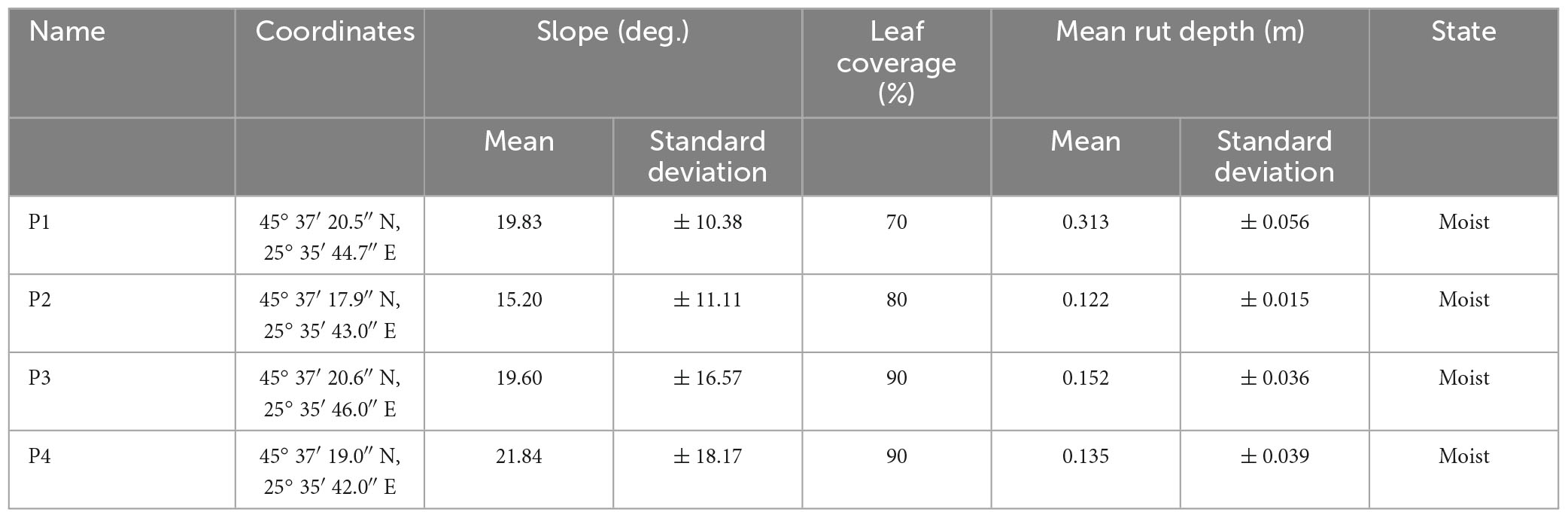
Table 1. Description of the sample plots.
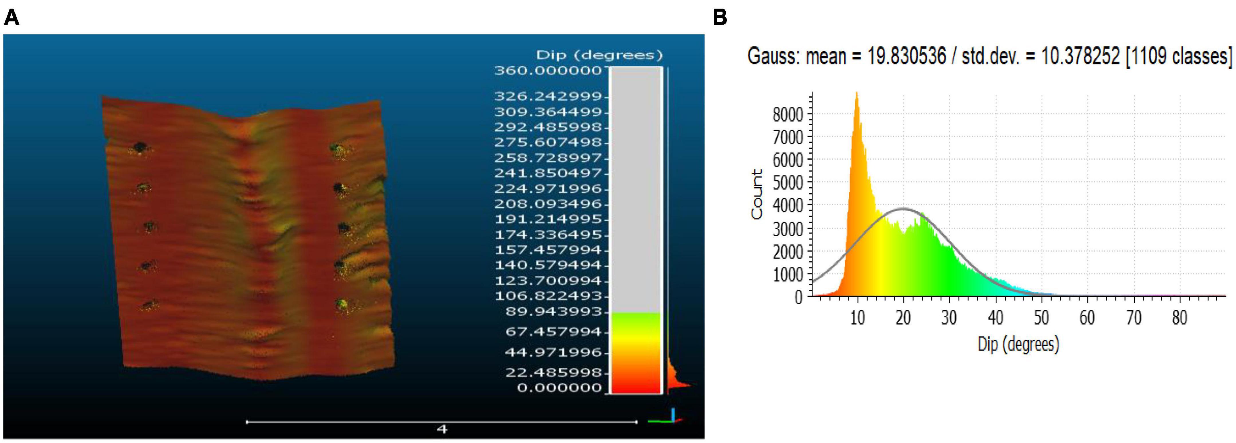
Figure 1. An example of color-coded point cloud (A) and histogram (B) showing slope in sample plot 1 (P1).
Data collection process was implemented in April 2022. The sample plots were rectangular in shape (Figure 1), measuring approximately 2 by 10 m and were geographically positioned using a handheld GPS receiver. Ten ground control points (GCP) were used in each plot, placed on their boundary and spaced at approximately 2 m each other (Figure 1), so as to form a grid overlapped on the boundary of each sample plot. GCPs were in the form of white plastic spheres, measuring 10 cm in diameter, attached to black stands, which were inserted vertically into the soil so as the top of each sphere was located at approximately 30 cm above the ground. These spheres were marked in advance on the sides with numbers from 1 to 10 by the use of a black permanent marker.
2.2. Acquisition and processing of LiDAR data
Two mobile LiDAR-based devices were used for scanning, namely the GeoSLAM Zeb-Revo (GeoSLAM Ltd et al., 2017) and the iPhone 13 Pro Max (Apple Inc., Cupertino, CA, USA, 2021). SiteScape and 3DScanner App were installed on the iPhone platform and used to collect the point clouds. The steps involved in the data collection process are illustrated in Figure 2. The scanning procedures used for the Zeb Revo were adapted to those used in earlier studies (Ryding et al., 2015; Gollob et al., 2021; Marra et al., 2022), meaning that the operator walked slowly around the edge of each sample plot, following a closed path while remaining about 1.5 m away from the boundary. This approach aimed to ensure that the entire area was scanned and to minimize position accuracy drifts and scanner range noise. After each scanning process and based on external control, the device automatically processed and saved the point cloud data on a USB stick. For the mobile phone and associated apps, scans were done at medium-density (MD), for which the clouds showed a good representation of the ground. The LiDAR sensor collected the 3D point cloud data as the operator walked along the plot’s axis. In each plot, two scans were taken by the Zeb Revo device; the iPhone platform was used to take two scans by 3D Scanner app, and another two by the SiteScape app. After each measurement day, the point clouds produced by both LiDAR platforms were transferred into a computer. Table 2 describes the point cloud datasets and their corresponding settings used in the C2C and data analyses.
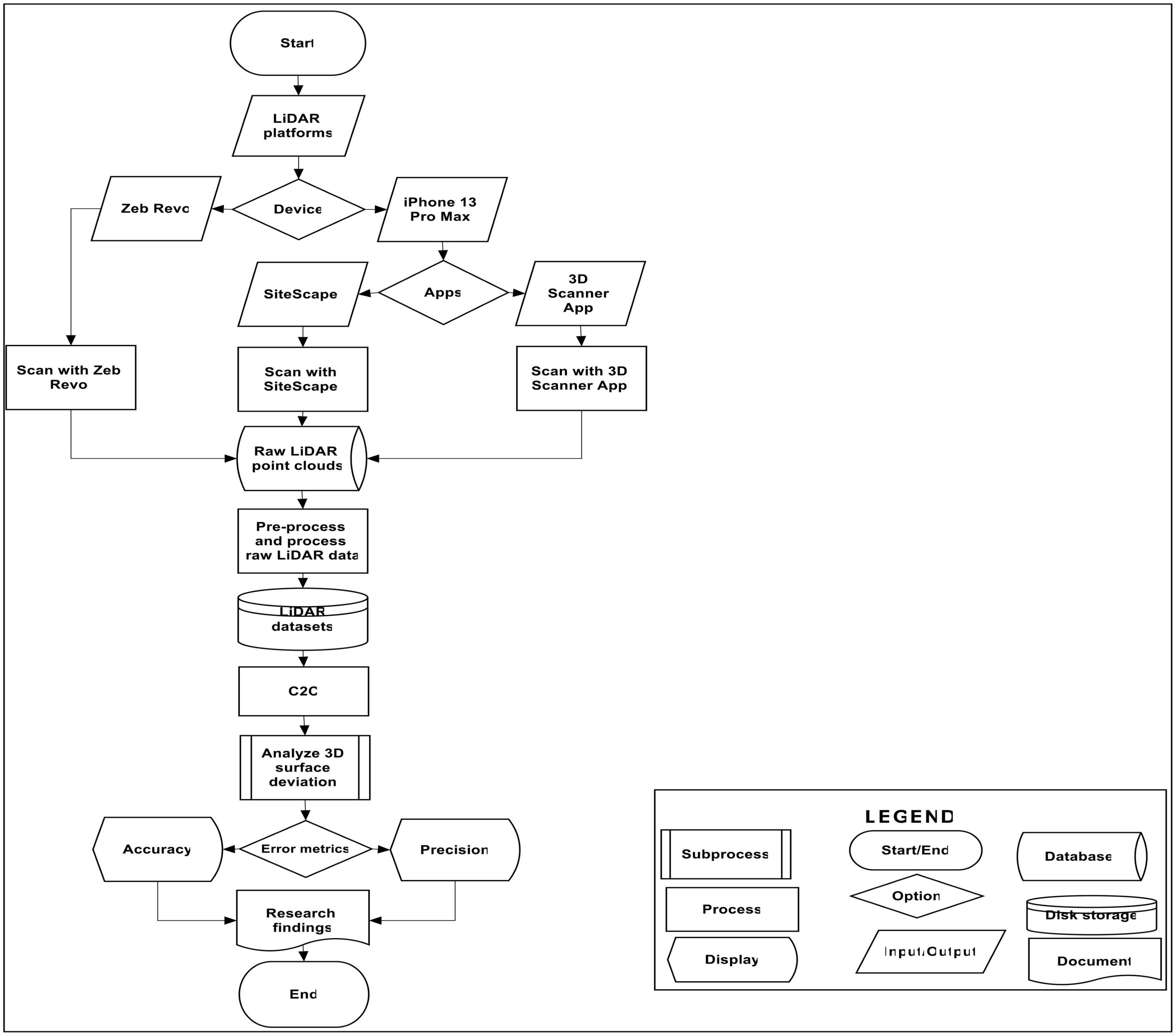
Figure 2. Flow chart of LiDAR data collection, processing, analysis and cloud-to-cloud comparison in CloudCompare software. Designed with ClickCharts diagram flowchart software Version 6.98. © NCH software.
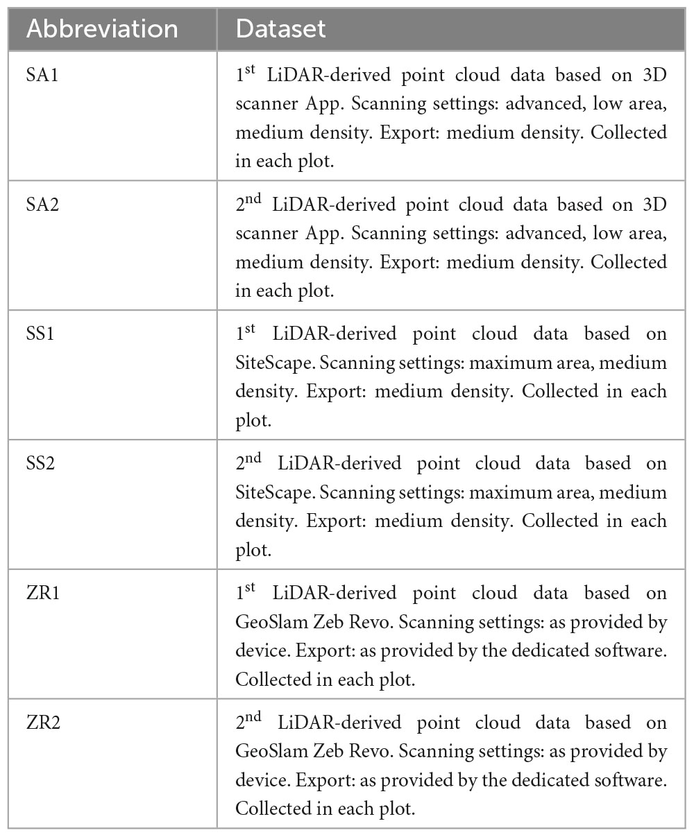
Table 2. Description of the datasets used in the C2C and data analyses.
Point clouds produced by scans had various sizes after pre-processing. Typically, the ZR files had between approximately 1.0 and 1.7 million points, SA between approximately 0.2 and 0.8 million points and SS between approximately 0.7 and 2.3 million points, respectively.
2.3. Cloud-to-cloud comparisons (C2C) of the point clouds
2.3.1. Point-cloud pre-processing and processing
The Cloud-to-Cloud comparison method (C2C) computes the distances between two LiDAR point clouds, and is a widely used technique (Ahmad Fuad et al., 2018). The C2C method compares a reference point cloud generated from a highly accurate surveying method to a test point cloud generated from the LiDAR system under test. This is done by aligning and comparing the point clouds to identify any discrepancies or potential errors in the data, and to estimate the accuracy and precision of the LiDAR system under test (Lague et al., 2013; Ahmad Fuad et al., 2018; Kharroubi et al., 2022). The accuracy and precision of the low-cost LiDAR platforms used for mobile scanning were estimated in this study using the C2C approach. Feature-based and Iterative Closest Point (ICP) options were combined as a part of the coarse-to-fine (C2F) registration strategy (Besl and McKay, 1992; Cheng et al., 2018). The feature-based method was used to identify the corresponding ground control points (GCPs) between the test and reference point clouds and align them accordingly as an initial coarse registration, while the ICP algorithm was used to find the closest point pair between the two-point clouds and align them together in a fine registration (Besl and McKay, 1992; Cheng et al., 2018). Cheng et al. (2018) claim that the fine registration approach is used to alter the results of coarse registration to acquire a satisfactory starting position. This is the main justification for using the two options in this study. Nevertheless, due to the iterative nature of point cloud registration, the ICP technique is slower in identifying connected points between two-point clouds and less effective at registering large, high-density point cloud files (Cheng et al., 2018).
In this study, C2C involved five stages: raw point cloud data pre-processing and processing, point cloud alignment, point cloud fine-registration, cloud-to-cloud distance computation, and surface deviation analysis in CloudCompare software (version 2.12 beta; Girardeau-Montaut, 2015). CloudCompare is a widely used software for point cloud processing, analysis, and visualization (Girardeau-Montaut, 2015; Ahmad Fuad et al., 2018). It provides a range of tools for cleaning, segmentation, filtering, aligning, registering, computing distances, and comparing point clouds (Biber and Strasser, 2003; Ahmad Fuad et al., 2018; Kharroubi et al., 2022). The raw point cloud data pre-processing and processing involved cleaning and segmentation. The point clouds were first imported from the LiDAR scans in a LAZ file format (.laz) (Thomson, 2018). The raw point cloud data acquired from all the mobile LiDAR scanning platforms were then processed by cleaning the 3D point cloud using the noise filter tool in CloudCompare, which removes unnecessary data associated with the scanned surface (Ahmad Fuad et al., 2018). After cleaning the clouds, the data were segmented using the interactive segmentation tool (Girardeau-Montaut, 2015), exported, and saved in PLY MESH (.ply) file format (Thomson, 2018). According to Rajendra et al. (2014), point cloud pre-processing and processing involve converting the initial raw LiDAR-derived point cloud into a final deliverable. For the purposes of this study, the final deliverables were fully cleaned and segmented LiDAR scans of the soil surfaces for the C2C.
2.3.2. Alignment of the processed LiDAR-derived point cloud
The ground control points (GCPs) found on each of the two clouds were first selected and then used for alignment (Maté-González et al., 2022). Iterative Closest Point (ICP), a popular approach that iteratively discovers the transformation parameters that minimize the distance between matching points in the two clouds, was used in CloudCompare to align pairs of point clouds (Besl and McKay, 1992). A rotation, translation, and scaling factor make up the rigid transformation. The objective was to identify the transformation parameters that would best align the point clouds (Besl and McKay, 1992). To create a statistically fair comparison, all point clouds used in the C2C were subsampled to 50,000 points (Costantino et al., 2022). Once the optimal transformation parameters were found, the clouds were aligned, and the registration process was complete. Then the RMS values, mean distance, and their standard deviations were recorded. The alignment quality was then assessed using various tools provided by CloudCompare, including color-coded deviation maps, distance histograms, and visualization of the aligned clouds. These tools enabled the evaluation of the accuracy and precision of the alignment and refinement of the alignment parameters if necessary. Figure 3 shows the ICP alignment process and results provided by the CloudCompare software. Typically, a satisfactory beginning position is initially attained using the point cloud alignment approach, and then registration is fine-tuned using the fine registration method (Biber and Strasser, 2003; Cheng et al., 2018).
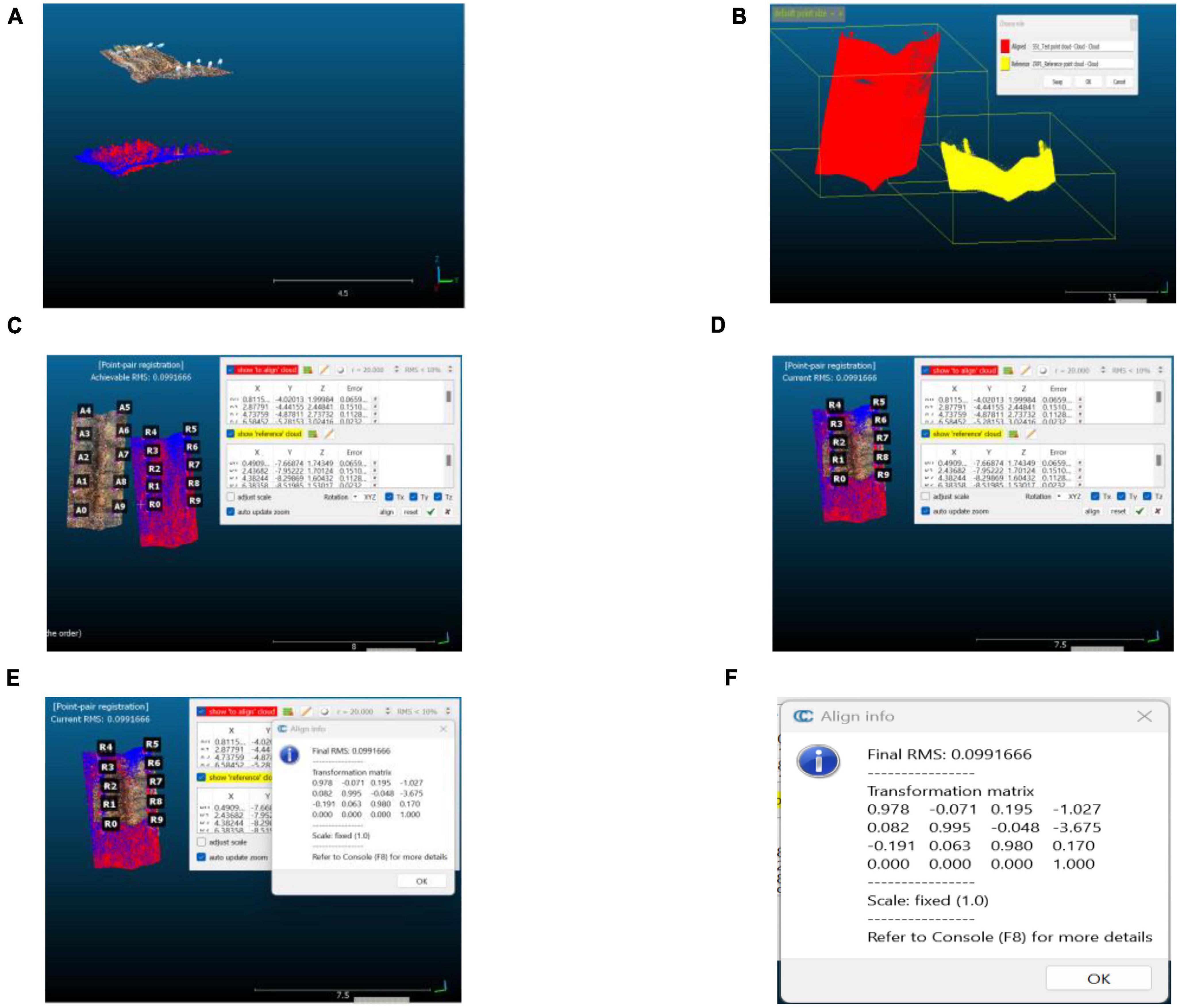
Figure 3. An example of ICP alignment and results using low-cost LiDAR-derived data collected by SiteScape (compared) and Zeb Revo (reference) point clouds for Plot 1: (A)–the point clouds before role selection, (B)–the selected test and reference point clouds, (C)–the point clouds ready for alignment after GCP picking, (D)–the aligned point clouds, (E)–the aligned point clouds with the alignment information, (F)–the alignment information on the final RMS error and transformation matrix.
2.3.3. Fine registration
The ICP registration method was used for the fine registration of the datasets. This method iteratively matches points in two datasets to find the optimal transformation that aligns the datasets (Segal et al., 2009). The ability to automatically complete the ICP registration process is provided by the CloudCompare program (Ahmad Fuad et al., 2018). However, the value for the point sample unit and the number of iterations were specified prior to starting the ICP registration procedure. Figure 4 shows an example of the CloudCompare’s results and the ICP registration options.
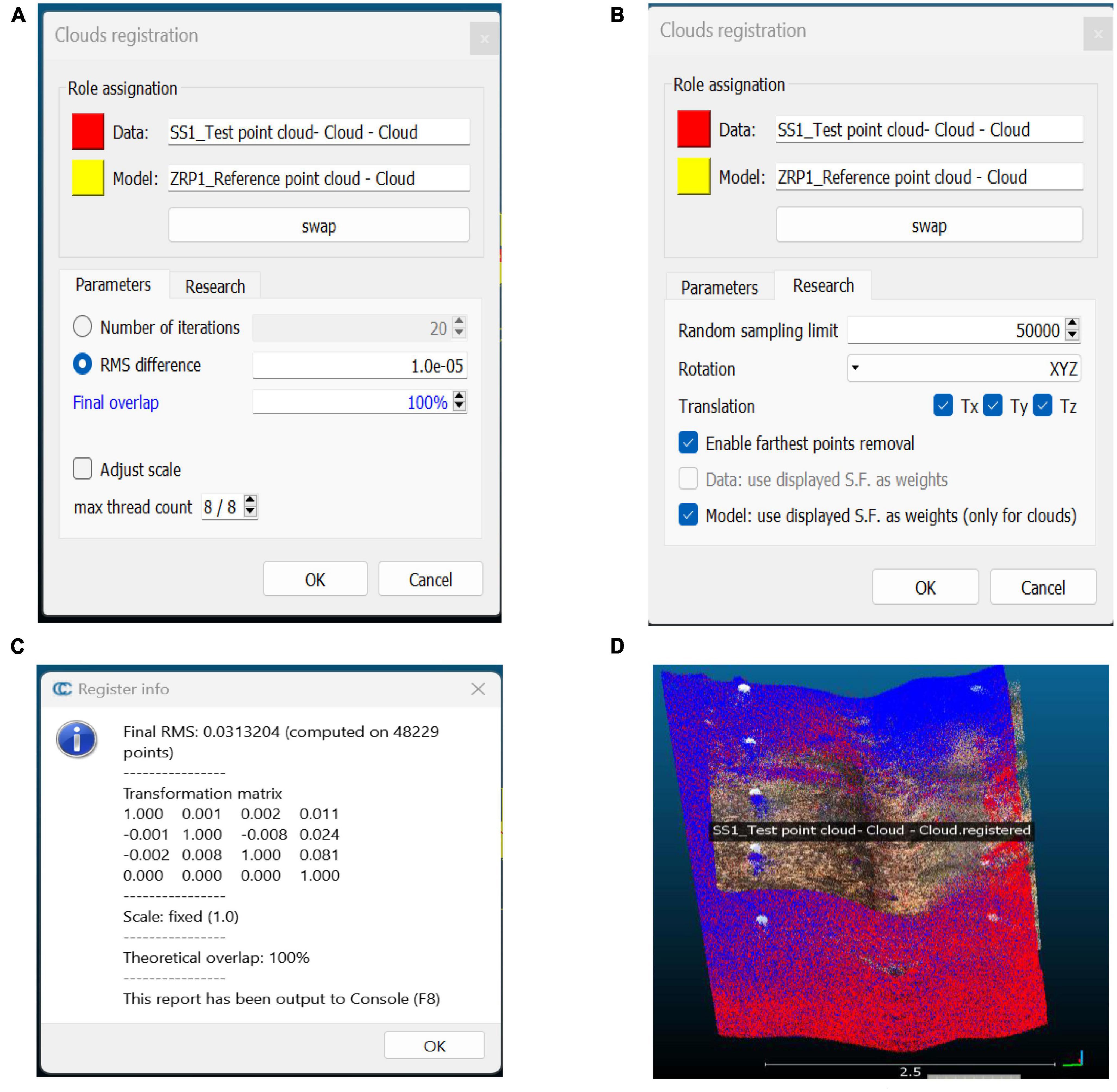
Figure 4. An example of ICP registration and results using low-cost LiDAR-derived data collected by SiteScape (compared) and Zeb Revo (reference) point cloud for Plot 1: (A)–the number of iterations and final overlap, (B)–the default number of sampling points, (C)–the final RMS error and the transformation matrix, (D)–the registered point cloud.
The registration method consisted of several steps, including point selection, point matching, transformation estimation, and transformation refinement. The first step was to select a subset of points from the two datasets. Here again, all point clouds used in the ICP method were those subsampled to 50,000 points (Figure 4B). These points were used as the initial correspondence between the two datasets. The point matching step involved finding the closest points in the second dataset for each point in the first dataset. This was done using the more robust Point-to-Plane distance measure (Rusinkiewicz and Levoy, 2001). For the accuracy and precision analyses, the number of iterations of the algorithm was fixed to the default value of 20, the optimum threshold for minimizing the root mean square (RMS) difference was 1.0 E-05 m, and the theoretical overlap was set 100% (Figure 4A). Following the establishment of the correspondences, the transformation estimation process involved determining the transformation that would best align the two datasets. This transformation was rigid, consisting of a rotation, a translation, and scale factor (Ahmad Fuad et al., 2018; Cheng et al., 2018). A least-square optimization was used to compute the transformation, minimizing the distance between equivalent points in the two datasets (Besl and McKay, 1992; Cheng et al., 2018).
Following the initial transformation, the transformation refinement step iteratively refined the transformation by repeating the point selection, point matching, and transformation estimation steps. The refinement process continued until convergence criteria were met, such as the change in the transformation parameters or the distance between corresponding points falling below a certain threshold. To align the two datasets, the approach iteratively matched points in each of the two datasets before computing the best rigid transformation (Zhang, 1994; Zhang et al., 2015).
To estimate the accuracy of the low-cost LiDAR technology in this study, the point clouds collected by SiteScape and 3D Scanner App were compared against those collected by Zeb Revo, using the Zeb Revo LiDAR point clouds as reference point clouds. For simplicity, the comparisons were done for each plot by matching the repetitions taken by iPhone with those taken by Zeb Revo, namely SA1 against ZR1, SS1 against ZR1, SA2 against ZR2 and SS2 against ZR2. Furthermore, the precision of each LiDAR platform was estimated in each plot by comparing the first repetition against the second one taken by the same platform and software, namely SA1 against SA2, SS1 against SS2 and ZR1 against ZR2. The RMS values, mean distances and their standard deviations were recorded once the registration process was complete.
2.3.4. Cloud-to-cloud distance computation and surface deviation analysis
The 3D surface deviation analysis was carried out using CloudCompare software with the C2C distance computation method (Zhang, 1994; Zhang et al., 2015; Ahmad Fuad et al., 2018). The software first estimates the results for the distance computation between the chosen datasets using the reference dataset and the compared dataset. Local surface model option from the local modeling menu of the CloudCompare was chosen to increase the accuracy of analysis. Computation was done by the Least Square Plane C2C distance with the default values. The appropriate Octree level value for the process was automatically determined (Zhang, 1994; Zhang et al., 2015; Ahmad Fuad et al., 2018). By activating the data in the layer panel, it was simple to see the resulting 3D surface deviation that was displayed and saved in the test datasets.
The outcome of the 3D surface deviation analysis was then used to identify any alterations resulting from the differences in the compared LiDAR datasets. The CloudCompare software comes equipped with a color scale that displays the value of the C2C distance computation to provide a better understanding of the result. The aligned and registered point clouds were then compared using various metrics, such as the root mean square (RMS), mean distances, and their standard deviations. The RMS error is the square root of the mean square error (MSE) between two clouds (Chai and Draxler, 2014; Brassington, 2017). These metrics help quantify the differences between the point clouds and provide insight into the accuracy and precision of the LiDAR data. However, the C2C distance computation process using CloudCompare software was susceptible to errors, such as the inclusion of unnecessary point cloud data that did not belong to the computed surfaces. To mitigate this for the low-cost LiDAR datasets, the point cloud cleaning and segmentation tools were used. Additionally, the most suitable filtering method was used to produce the point clouds datasets that only belonged to the soil surface (Ahmad Fuad et al., 2018). It is important to note that the accuracy of the analysis was improved by carefully selecting the appropriate filtering methods and settings.
3. Results and discussion
3.1. Accuracy of low-cost derived point clouds
The results on the accuracy of low-cost mobile LiDAR scans using the C2C in the studied plots are summarized in Figure 5 and Table 3. Figure 5 gives only a limited amount of information on the accuracy comparisons. For more graphical information, see the Supplementary material. For the comparison of SS1 against ZR1 in Plot 1 (Figure 5), these metrics were computed on 47,372 points out of 50,000 subsampled from approximately 1.37 million sampling units of the SS test point cloud (Figures 5A, C). The results indicated that the mean distance was 0.010 m, with standard deviation of 0.009 (Figure 5E). Additionally, the final RMS errors during point cloud alignment and fine registration were 0.030 and 0.093 m, respectively (Table 3). For the C2C of SA1 against ZR1 point clouds in the same sample plot (Figures 5B, D, F), however, the metrics were computed on 46,828 points out of the 50,000 points selected from 337,086 sampling points of the SA test point cloud (Figures 5B, D). The results indicated that the mean distance was 0.004 m at a standard deviation of 0.005 (Figure 5F). Moreover, the final RMS error of the registration phase was 0.018 m, while the final RMS error obtained during the alignment phase was 0.042 m (Table 3).
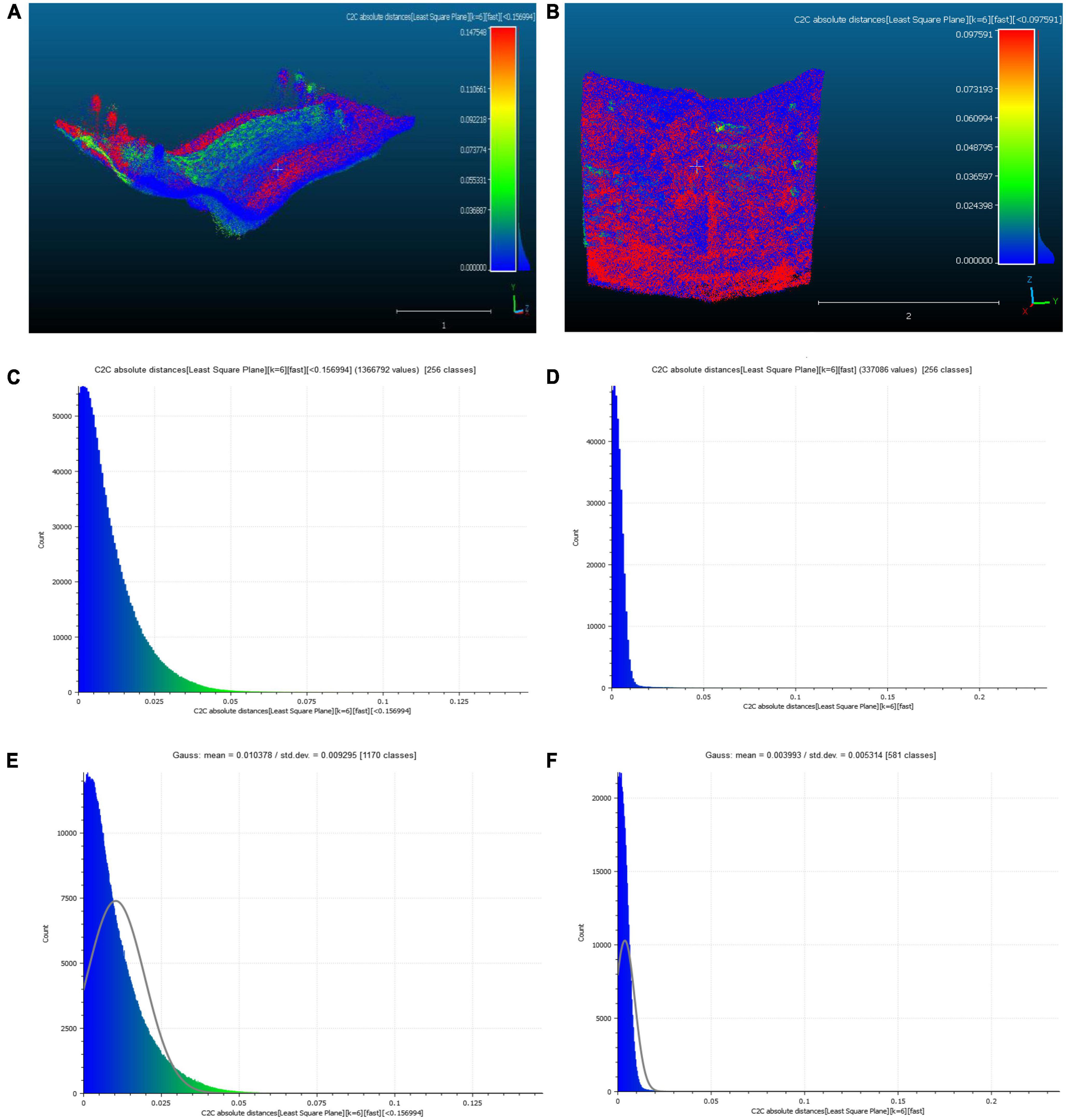
Figure 5. An example of accuracy in terms of observed differences between SS1 and ZR1 in Plot 1 (A,C,E) and between SA1 and ZR1 in Plot 1 (B,D,F): (A,B)–color-coded deviation map of absolute distances, (C,D)–histogram of absolute distances, (E,F)–histogram of the mean distance and standard deviation.
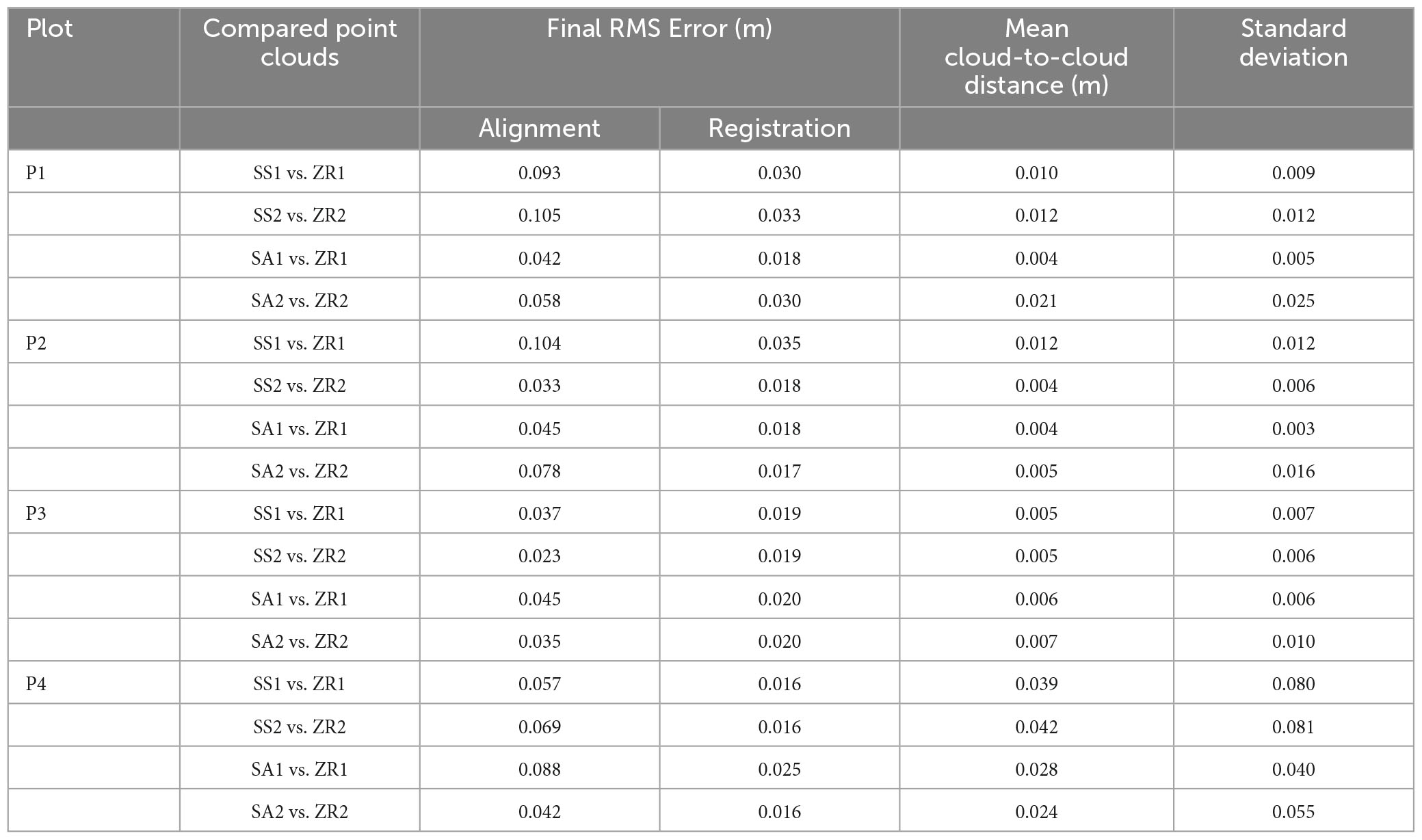
Table 3. Summary statistics of C2C showing the accuracy of the LiDAR scans.
Similar results on accuracy were obtained in the remaining C2Cs of SS and SA against the ZR reference point cloud. Table 3 provides a summary of all the results on accuracy of the LiDAR scans with SS and SA by considering the sample plot under question, RMS error obtained at the alignment and registration phases, as well as the mean and standard deviation of distance calculations between point clouds. As shown, the SA had lower RMS errors, mean distances and standard deviations compared to the SS, indicating that it may be more accurate in measuring distances with better repeatability. From these results, the range of final RMS errors of SS vs. ZR was 0.016–0.035 m (Range = 0.019 m). Additionally, the average final RMS error of SS vs. ZR was 0.023 m. In terms of the mean cloud-to-cloud absolute distance, the values varied from 0.004 to 0.039 m (Range = 0.035 m). The corresponding the standard deviation values varied from 0.003 to 0.081 (Range = 0.078). However, the average cloud-to-cloud distance and average standard deviation of SS vs. ZR were 0.016 m and 0.032, respectively.
For SA vs. ZR, the final RMS errors varied from 0.017–0.025 m (Range = 0.007 m). Moreover, the average final RMS error of SA vs. ZR comparisons was 0.020 m; the mean distance varied from 0.004 to 0.042 m (Range = 0.038 m). The corresponding standard deviation varied from 0.006 to 0.081 (Range = 0.075). However, the average cloud-to-cloud absolute distance and average standard deviation values of SA vs. ZR comparisons were 0.011 m and 0.021, respectively.
Overall, both SA and SS produced relatively accurate point clouds with low RMS errors, but SA appeared to have a slight edge in terms of consistency (repeatability) and smaller errors. The overall average final RMS error for SS was slightly higher than the overall average for SA (0.023 vs. 0.020 m). Besides, the SA has a slightly lower average mean distance and standard deviation compared to the SS, indicating that on average, the SA may be slightly more accurate than SS for cloud-to-cloud comparisons using the ZR as the reference point cloud. The results also suggest that the SA has less variability in its measurements than the SS and therefore greater repeatability by comparing the average standard deviations (0.021 vs. 0.032 m). The difference in accuracy between the two apps is relatively small, so it may not be a significant difference and thus suggesting that both apps are comparable in terms of overall accuracy.
3.2. Intercloud precision of the LiDAR-derived point clouds
Figure 6 and Table 4 show the results of the precision of low-cost mobile LiDAR scans. Figure 6 shows the results graphically only for the sample plot 1. The rest of the graphical results are given in the Supplementary material. The final RMS errors, mean distance, and standard deviation were used to evaluate the precision of the scans during both the alignment and registration phases. For instance, the comparison of SS1 and SS2 in Plot 1 (Figure 6) was based on 46,091 points out of 50,000 points subsampled from approximately 1.37 million of sampling units of SS test point cloud (Figures 6A, D). The results indicated that the mean distance was 0.006 m at a standard deviation of 0.009 m (Figure 6G). The final RMS error in registration was 0.017 m, whereas the final RMS error obtained during the alignment phase was 0.074 m (Table 4). Similarly, the statistical metrics for the C2C of SA1 and SA2 in the same sample plot 1 (Figure 6) were computed on 44,378 points out of 50,000 subsampled from approximately 0.83 million sampling units of the SA test point cloud (Figures 6B, E). The mean distance was 0.005 m with a standard deviation of 0.014 m (Figure 6H). Additionally, the final RMS error at fine registration was estimated at 0.012 m, whilst the final RMS error at the alignment phase was 0.039 m (Table 4). Regarding ZR1 and ZR2 C2C in the same sample plot 1 (Figure 6), the metrics were computed on 39,273 points out of 50,000 points selected from approximately 1.23 million sampling units of the ZR test point cloud (Figures 6C, F). The mean distance was 0.057 m, and the standard deviation was 0.185 m (Figure 6I); the final RMS error at fine registration was estimated at 0.019 m, while the final RMS error obtained during the alignment phase was 0.053 m (Table 4). A summary of all the comparisons is presented in Table 4.
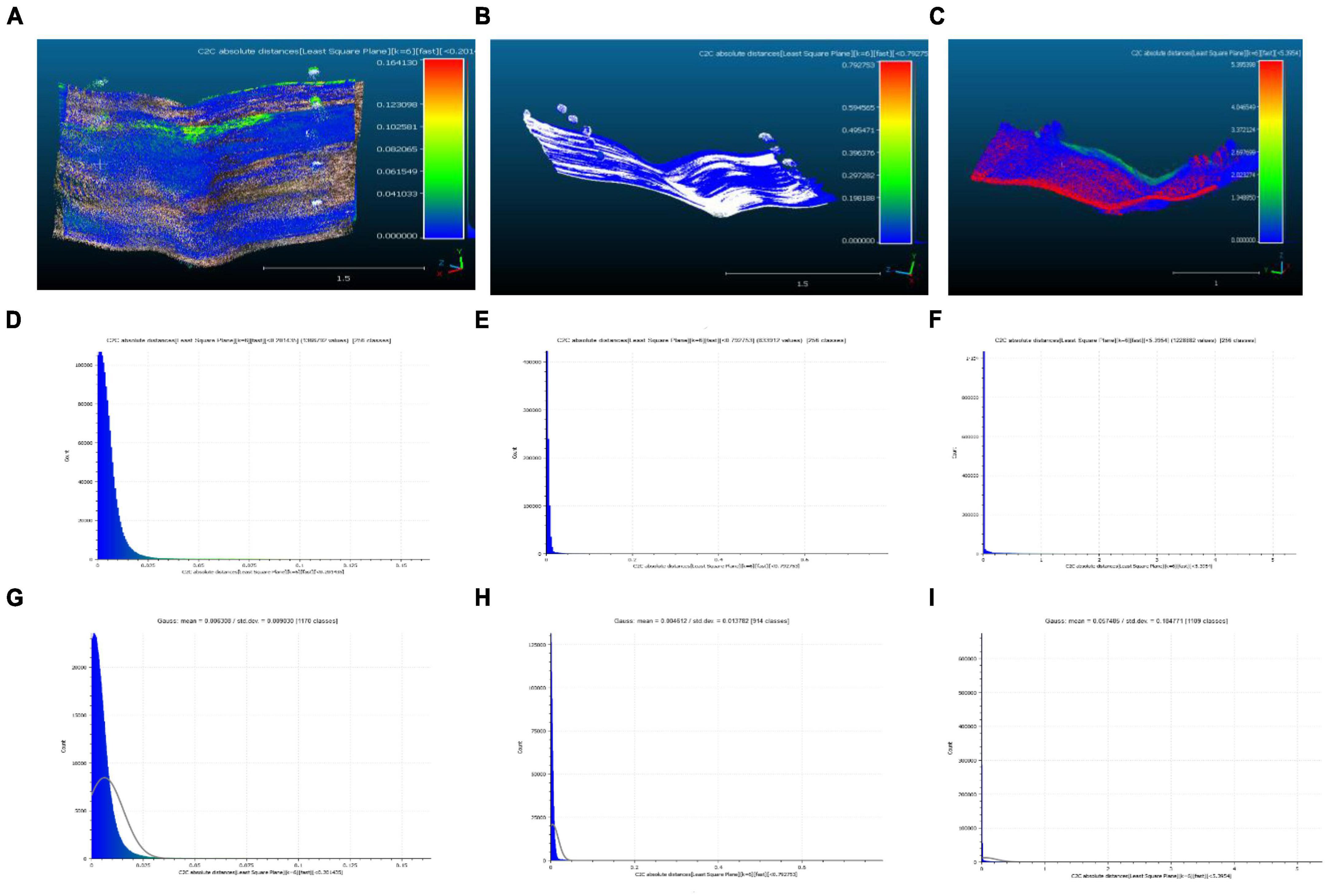
Figure 6. An example of precision in terms of observed differences of SS1 and SS2 (A,D,G), between SA1 and SA2 (B,E,H) and between ZR1 and ZR2 (C,F,I) in Plot 1: (A–C)–color-coded deviation map of absolute distances, (D–F)–histogram of the C2C absolute distances, (G–I)–histogram of the mean distance and standard deviation.
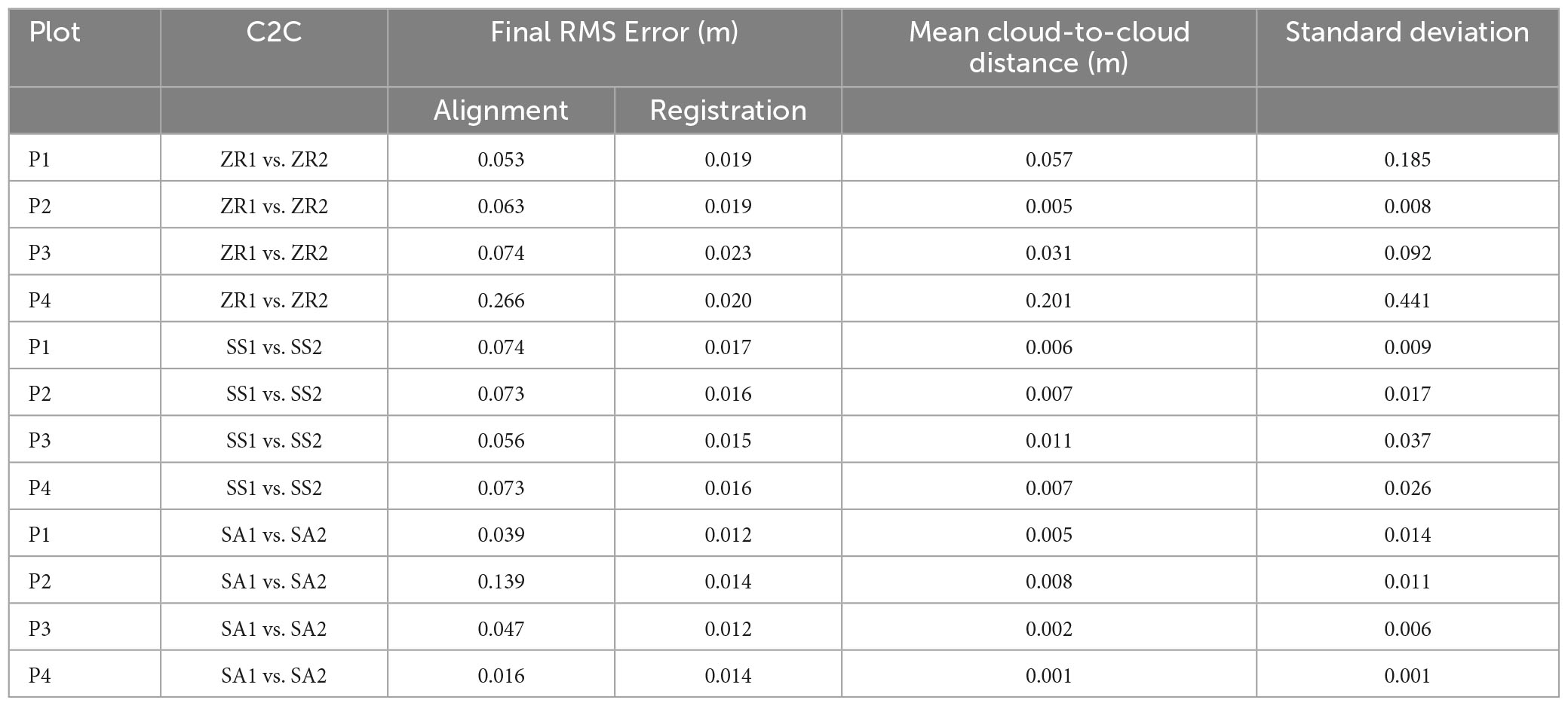
Table 4. Summary statistics of C2C showing the precision of the LiDAR scans.
The results presented in Table 4 show the final RMS errors at point cloud alignment and registration, and the mean C2C (cloud-to-cloud) absolute distances and their standard deviations of the point clouds generated by the iPhone 13 Pro Max (Apple Inc., 2021b) equipped with SS and SA and the professional mobile LIDAR platform of ZR for the four sample plots. From these results, the final RMS error values at fine registration when comparing ZR1 with ZR2 varied from 0.019 to 0.023 m (Range = 0.004 m). Additionally, the average final RMS error of ZR1 vs. ZR2 was 0.021 m. In terms of the range of values for the mean distance and standard deviation for ZR1 vs. ZR2, the mean distance varied from 0.005 to 0.201 m (Mean distance range = 0.197 m), and the standard deviation varied from 0.008 to 0.441 (Standard deviation range = 0.028). Similarly, the average cloud-to-cloud distance and standard deviation of these comparisons were 0.074 and 0.181 m, respectively.
For the comparison between SS1 and SS2, the final RMS error values varied from 0.015 to 0.017 m (Range = 0.002). The average RMS error of SS1 vs. SS2 was 0.017 m. Furthermore, the mean distance varied from 0.006 to 0.011 m (Mean distance range = 0.004 m), while the standard deviation varied from 0.009 to 0.037 m (Standard deviation range = 0.028); the average cloud-to-cloud distance was 0.008 m with a standard deviation of 0.023 m. Regarding the comparison between SA1 and SA2, the final RMS error values varied from 0.012 to 0.014 m (Range = 0.002 m). Moreover, the average RMS error of SA1 vs. SA2 was 0.013 m. Additionally, the mean distance ranged from 0.001 to 0.008 m (Mean distance range = 0.007), and the standard deviation ranged from 0.001 to 0.014 m (Standard deviation range = 0.012). However, the average cloud-to-cloud distance and standard deviation of these comparisons were 0.004 and 0.009 m, respectively.
Generally, these results suggest that the precision of the low-cost mobile LiDAR technology in estimating soil disturbance in forest operations is high. The final RMS errors, mean distances and standard deviations observed during the C2C comparison were generally low, indicating a high degree of precision. However, the results also show that the final RMS errors during the alignment phase were higher than during the registration phase. Overall, these results suggest that the SA app installed on the iPhone was the best option in terms of precision and consistency (repeatability).
3.3. Discussion
This study aimed to estimate the accuracy and precision of the low-cost mobile LiDAR technology in estimating soil disturbance in forest operations using a cloud-to-cloud comparison approach (C2C), and on that basis, to give indications on repeatability. Regarding the metrics for estimating the accuracy and precision in this study, the RMS error and standard deviation are very similar statistical measures of variability (accuracy, precision, and repeatability) used in LiDAR research (Carter et al., 2012). However, studies show that the two values will be equal in a non-biased data set, when the error is normally distributed above and below zero (Carter et al., 2012). The closer the average RMS error values to zero, the better the performance, as it indicates a smaller deviation from the actual values (Girardeau-Montaut et al., 2005; Ahmad Fuad et al., 2018). Similarly, the lower the average cloud-cloud distance values, the better the accuracy and precision of the scanning device and technology used (Girardeau-Montaut et al., 2005; Ahmad Fuad et al., 2018). According to MacMillan et al. (2023), the standard deviation provides a sense of how close the complete collection of data is to the average value; data sets with modest standard deviations contain precisely organized data, while those with big standard deviations have data dispersed throughout a wide range of values. For example, if the standard deviation of a measurement is very small, it means that repeating that measurement will give similar results. Thus, lower values of the average standard deviation in this study indicate less variability in the precision and accuracy of the scanning devices and therefore greater repeatability.
In this study, the final alignment and registration RMS errors represent the error in aligning the SS and SA scan point clouds and registering them to the reference ZR point cloud, respectively. These errors were used to quantify the difference between test and reference point clouds, and subsequently estimate the accuracy and precision. These values gave us an idea of the variability of the registration and alignment accuracy and precision for each application and device. Nonetheless, the average standard deviation values showed how much the scanned data was spread out from the mean cloud-to-cloud distances, which were used to assess the repeatability of this method. Additionally, the mean cloud-to-cloud distance is the average displacement between the SS or SA point clouds and the reference model of ZR in each plot, which also gave us an idea of the accuracy and precision of the low-cost mobile LiDAR technology.
Overall, the performance of each application in terms of accuracy varied plot wise. SA consistently had the smallest final RMS error values, indicating that it was more accurate in capturing the geometry of the reference model. However, SA had considerably higher final RMS error values, especially in P4, which suggests that it may have some limitations in capturing more complex geometries (see Supplementary material). SS had the lowest overall mean cloud-to-cloud distance and standard deviation in P2. However, it had considerably larger final RMS error values in P1 and P4, suggesting that it is less accurate in capturing certain types of geometries. Similarly, based on the ranges of RMS errors, SA performed slightly better in terms of accuracy compared to SS. SA had a narrower range of RMS errors, which means that the errors varied less between different test point clouds. In contrast, SS had a wider range of RMS errors, indicating that its accuracy varied more between different test point clouds. However, SA’s RMS errors were generally smaller than SS’s RMS errors. SA’s lowest RMS error (0.017 m) was smaller than both of SS’s RMS errors, and SA’s highest RMS error (0.025 m) was still smaller than SS’s highest RMS error (0.035 m). This suggests that SA may be more consistently accurate across different test conditions, while SS may be less predictable in terms of accuracy.
In general, the registration error was smaller than the alignment error across all plots for all applications, suggesting that the registration process was generally more accurate. Overall, these results suggest that both applications can be useful for capturing 3D geometry of soil disturbance in forest operations. However, the accuracy of each application may vary based on the complexity of the soil geometry being captured as well as the complexity of space surrounding the sample plots. Further research could focus on identifying the limitations of each application and developing methods for improving the accuracy of 3D scanning.
Based on the average (mean) distance and standard deviation, SA had a slightly lower average mean distance and standard deviation compared to SS, indicating that it may be slightly more accurate. Overall, the average standard deviations for both apps were relatively low, indicating that they may have good repeatability on average. However, the standard deviations for some of the individual comparisons were relatively large (e.g., SS2 vs. ZR2 in P4 with a standard deviation of 0.081 and SA2 vs. ZR2 in P2 with a standard deviation of 0.016), indicating a lower repeatability in those cases. This suggests that while the studied apps may have good repeatability on average, there are some individual cases where the results could be less reliable. It is possible that this is due to differences in the underlying algorithms or hardware used by each application and device (Gollob et al., 2020, 2021). Further analysis, such as statistical testing or confidence interval estimation, could be used to better understand the variability of the results and their implications for the application being studied. Besides, comparing the average standard deviation values with the average RMS error values, it is evident that for all applications and plots, the standard deviation values were significantly lower. This suggests a good consistency and repeatability in the measurements, and a low uncertainty in the obtained results (Downing, 2004; Nakagawa and Schielzeth, 2010).
The overall accuracy and performance of each application and device may vary depending on the specific use, precision of the data, and other factors. Based on the results of this study, it appears that both applications can achieve a reasonable level of accuracy for cloud-to-cloud comparisons. Therefore, the choice of a given application may ultimately depend on other factors such as precision, user preferences, cost, and ease of use (Wang and Qi, 2021).
Similarly, the study found that the precision of SS, SA, and ZR point clouds was high. The ranges in the descriptive statistics indicated the variability in the final RMS error values, mean cloud-to-cloud absolute distances, and their standard deviation values for each application and device across all four plots; they shown that comparisons between SA1 and SA2 had the least variability in RMS error values, while the ZR1 vs. ZR2 comparisons had the highest variability. Moreover, the SA1 vs. SA2 C2C had the lowest range of values for both mean distance and standard deviation, indicating that the SA application was a consistent (repeatable) and reliable option. The ZR1 vs. ZR2 C2C had the highest range of values for both mean distance and standard deviation, indicating that ZR was the least consistent (repeatable) option. The SS1 vs. SS2 C2C falls somewhere in between with moderate performance in terms of precision and consistency (repeatability).
However, the range alone does not provide enough information about the overall precision; the average of the final RMS error values, mean distance and standard deviation may give a more accurate representation. Consequently, both the range and the average values were combined in the overall evaluation of the performance of the LiDAR platforms. From the results, SA1 vs. SA2 C2C had the lowest average RMS error (0.013 m), indicating that 3D Scanner app was the most precise option. The SA1 vs. SA2 had also the lowest average mean distance (0.004 m), and standard deviation value (0.009), indicating that 3D Scanner app was the most consistent (repeatable) option. On the other hand, the ZR1 vs. ZR2 C2C had the highest average RMS error (0.021 m), which suggests that it was the least precise option. Moreover, the ZR1 vs. ZR2 has the highest average mean distance (0.074 m), and the highest standard deviation (0.181), which suggests that this option was the least consistent (repeatable).
There is limited information available on similar studies for direct comparisons of these findings. For instance, SiteScape is supposed to enable users to easily take 3D scans that are accurate to within ± 1 inch, on average (Corke, 2021). Findings of this study are consistent with some previous research that also used LiDAR systems and/or C2C comparison methods to estimate the accuracy and precision of LiDAR technology. For instance, Milenković et al. (2015) evaluated the accuracy and potential of terrestrial laser scanning (TLS) for soil surface roughness assessment. Their study found that TLS provided highly accurate measurements of soil surface roughness with a mean difference of 0.52 mm between TLS data and ground truth measurements. Furthermore, Mikita et al. (2022) investigated the use of different types of laser scanning methods, including the iPhone 12 Pro Max LiDAR scanning apps, for assessing damage to forest road wearing courses. The study found that the root mean square error (RMSE) of the iPhone LiDAR scanning method was 0.023 m and the coefficient of variation (CV) for the vertical accuracy of the iPhone LiDAR scanning method was 0.25%. They compared these values to those obtained using a terrestrial laser scanner (TLS) and a mobile laser scanning system (MLS). They found that the RMSEs and CVs of the iPhone LiDAR scanning method were comparable to those of the TLS and MLS, indicating that the iPhone LiDAR scanning method can provide accurate and precise measurements. Additionally, the study suggested that the iPhone apps have the potential to streamline the data acquisition process and reduce costs compared to traditional terrestrial laser scanning methods. Similarly, Luetzenburg et al. (2021) evaluated the Apple iPhone 12 Pro LiDAR for its potential application in geosciences. The study found a mean horizontal error of 0.03 m and a mean vertical error of 0.05 m in a vegetation-dominated environment, making it suitable for high-resolution topographic mapping applications. Additionally, Jaboyedoff et al. (2009) used terrestrial laser scanning for the characterization of retrogressive landslides in sensitive clay and rotational landslides in riverbanks, finding that this method was highly accurate and precise for monitoring landslide movement and deformation. The study reported accuracy values generally less than 5 cm and precision values ranging from 1 to 2 cm. Ahmad Fuad et al. (2018) also found that the Iterative Closest Point (ICP) registration method and the Least Square Plane cloud-to-cloud distance approach were more accurate than other methods for spotting changes in 3D landslide surfaces utilizing Mobile Laser Scanning data between two periods.
In general, the quality of the scan would depend on various factors such as the type of soil, its moisture content, and the texture but when it comes to scanning soil, one important consideration is the resolution of the scanner (Jaboyedoff et al., 2009; Milenković et al., 2015). According to a study by Milenković et al. (2015), the accuracy of laser scanning for soil surface roughness measurement was affected by the point density of the laser scanner. TLS was also found to have high spatial resolution and could be used as a valuable tool for monitoring soil erosion and other environmental changes (Milenković et al., 2015). Similarly, a study by Jaboyedoff et al. (2009) found that increasing the point density resulted in a significant reduction of the error in comparisons between terrestrial laser scanning datasets which was approximately 3 to 6 cm in their study. Therefore, a higher resolution scanner is likely to provide more accurate results when scanning soil surfaces. Another factor that could have affected the accuracy and precision of the low-cost LiDAR scans in this study was the presence of vegetation or other objects on the soil surface (Salmivaara et al., 2018). Several studies indicated that the presence of small vegetation and litter on the soil surface caused errors in the determination of soil surface elevation and roughness, compaction and rutting using LiDAR and TLS methods (Milenković et al., 2015; Salmivaara et al., 2018; Mohieddinne et al., 2022). According to Magtalas et al. (2016), the meter level distances and standard deviations in their study were produced by the fact that both point clouds’ whole contents including vegetation were used to calculate the cloud-to-cloud distance when they employed distance computations to further compare their findings. However, the descriptive statistics they used to assess accuracy and precision reduced when the C2C was performed on non-vegetation point clouds using the same procedure. Thus, the vegetation growing on the soil’s surface, which exhibited elevation differences of a few meters between the two datasets, might be the source of the meter level deviations (Magtalas et al., 2016). The accuracy and precision values from their study cannot, however, be directly compared to those from this study, because their technique of assessing the accuracy and precision differs from that used herein. Thus, further research is necessary to explore the effects of vegetation on the accuracy and precision of these low-cost LiDAR systems.
Despite being a useful method for analyzing LiDAR data, the C2C has important limitations in its use (Girardeau-Montaut et al., 2005; Cheng et al., 2018; Kharroubi et al., 2022). One of the main limitations is the assumption that the point clouds being compared are of the same geographic location. The comparisons may be inaccurate if there are any variations in the position or orientation of the point clouds during scanning (Girardeau-Montaut et al., 2005; Lague et al., 2013; Kharroubi et al., 2022). Additionally, the accuracy and precision of the cloud-to-cloud comparison method depend on the quality and resolution of the point clouds generated by the LiDAR systems (Cheng et al., 2018; Kharroubi et al., 2022). The C2C method is not robust to changes in point density and point cloud noise (Girardeau-Montaut et al., 2005; Lague et al., 2013), which may affect the accuracy and precision of the results. The accuracy of the method can be reduced if the clouds from different LiDAR systems have different point densities (Cheng et al., 2018; Kharroubi et al., 2022). These problems were addressed in this study by modeling the soil surfaces locally to prevent problems with density change.
Moreover, this study is constrained by the small sample size because it only included four rectangular plots, each measuring around 20 m2. More studies may be necessary to evaluate the suitability of this technology in different forested landscapes. Furthermore, the studies cited in this research paper are case studies and may not be generalizable to other locations or forest types. As such, additional research may be necessary to test the applicability of low-cost mobile LiDAR technology in other forested areas. In addition, the cost of high-end LiDAR systems for soil disturbance estimation may not be justifiable for small-scale forest operations. The potential benefits of low-cost mobile LiDAR technology for these operations may be limited by their accuracy and dependence on mobile platforms.
Numerous studies demonstrate that attaining accurate results with low-cost LiDAR technology depends on several variables, including the calibration parameters of the LiDAR platform components, the underlying point cloud density, the scanning settings, and the data processing methods used. Therefore, it is necessary to keep exploring new low-cost LiDAR technologies as they appear. Future studies might consider integrated low-cost LiDAR systems that can potentially offer enhanced capture options with a greater spatial resolution and a longer effective range in forest environments. Additionally, increasing plot coverage while maintaining low operational costs can potentially be achieved by designing and implementing a multiplatform LiDAR sensor solution using Apple’s iPhones. For instance, the use of selfie sticks in future research can potentially increase plot coverage and point cloud capture. Moreover, incorporating a multiple-iPhone strategy for the capturing of LiDAR point clouds may be able to shorten the time required for data collection. However, future studies should assess how quickly (time efficiency) point cloud data can be captured and processed using low-cost LiDAR technology. Besides, it will be necessary for extra caution to be taken in using the point picking tool in CloudCompare to ensure that the exact centers of the GCPs are hit to ensure proper alignment and subsequent registration of the point clouds.
Additionally, both the procedures and protocols used in low-cost LiDAR scanning and the experience of the operator are relevant factors that can impact the quality (accuracy, precision, and repeatability) of the resulting LiDAR data (Rathore, 2017). Several studies suggest that that optimizing the scanning procedure, by carefully planning the survey area, selecting appropriate scanning parameters and designing efficient scan paths, choosing the scanning pattern and processing of the data collected are essential steps in the process and can improve the quality of the data while reducing costs (Rathore, 2017; Wang and Menenti, 2021). The experience of the operator is also critical in ensuring the quality of data collected by low-cost LiDAR systems. An experienced operator can anticipate problems that may arise during the survey and adjust the scanning plan accordingly. Additionally, an experienced operator can make a significant difference in the accuracy of the data collected, particularly in areas with dense vegetation cover by understanding the limitations of the technology and taking appropriate corrective actions.
4. Conclusion
This study aimed to evaluate the accuracy and precision of three LiDAR options for estimating small-scale soil disturbance in forest operations. The three LiDAR options used can generate highly accurate and precise point clouds for small-scale soil disturbance estimation. The cloud-to-cloud distances (C2C) between the point clouds were generally small, indicating a high degree of similarity and agreement between the different options. However, some differences in accuracy and precision may exist between these options depending on the specific test conditions. Additionally, the precision of the LiDAR scans generated by the three options was generally good for all plots tested. The C2C distances between point clouds generated from the same option were also small, indicating a high degree of repeatability and consistency of the LiDAR scans for small-scale soil mapping. Overall, the study suggests that LiDAR scans generated by the three options are highly accurate and precise for small-scale soil disturbance mapping. Additional research is necessary to further validate the applicability of low-cost mobile LiDAR technology for mapping and monitoring forested landscapes.
Data availability statement
The raw data supporting the conclusions of this article will be made available by the authors, without undue reservation.
Author contributions
SB: conceptualization, supervision, and project administration. GF and SB: methodology, formal analysis, writing—original draft, writing–review and editing, resources, and funding acquisition. GF: data curation, validation, visualization, and investigation. Both authors contributed to the article and approved the submitted version.
Funding
This work was supported by the Transilvania University of Brasov–grant “Proiectul Meu de Diploma 2022,” which supported the purchase of some of the equipment used in the field data collection. Some of the activities of this study were supported by a grant of the Romanian Ministry of Education and Research, CNCS—UEFISCDI, project number PN-III-P4-ID-PCE-2020-0401, within PNCDI III.
Acknowledgments
We would like to thank Jenny Magaly Morocho Toaza for her help in the field data collection stage. We would also like to thank the Department of Forest Engineering, Forest Management Planning, and Terrestrial Measurements, Faculty of Silviculture and Forest Engineering, Transilvania University of Brasov, for providing some of the equipment needed for this study.
Conflict of interest
The authors declare that the research was conducted in the absence of any commercial or financial relationships that could be construed as a potential conflict of interest.
Publisher’s note
All claims expressed in this article are solely those of the authors and do not necessarily represent those of their affiliated organizations, or those of the publisher, the editors and the reviewers. Any product that may be evaluated in this article, or claim that may be made by its manufacturer, is not guaranteed or endorsed by the publisher.
Supplementary material
The Supplementary Material for this article can be found online at: https://www.frontiersin.org/articles/10.3389/ffgc.2023.1224575/full#supplementary-material
References
Ahmad Fuad, N., Yusoff, A. R., Ismail, Z., and Majid, Z. (2018). Comparing the performance of point cloud registration methods for landslide monitoring using mobile laser scanning data. ISPRS Arch. 42, 11–16. doi: 10.5194/isprs-archives-XLII-4-W9-11-2018
Akay, A. E., Oğuz, H., Karas, I. R., and Aruga, K. (2009). Using LiDAR technology in forestry activities. Environ. Monit. Assess. 151, 117–125. doi: 10.1007/s10661-008-0254-1
Ampoorter, E., de Schrijver, A, van Nevel, L, Martin Hermy, M., et al. (2012). Impact of mechanized harvesting on compaction of sandy and clayey forest soils: Results of a meta-analysis. Ann. For. Sci. 69, 533–542. doi: 10.1007/s13595-012-0199-y
Ampoorter, E., Van Nevel, L., De Vos, B., Hermy, M., and Verheyen, K. (2010). Assessing the effects of initial soil characteristics, machine mass and traffic intensity on forest soil compaction. For. Ecol. Manag. 260, 1664–1676.
Andrachuk, M., Marschke, M., Hings, C., and Armitage, D. (2019). Smartphone technologies supporting community-based environmental monitoring and implementation: A systematic scoping review. Biol. Conserv. 237, 430–442.
Apple Inc (2021a). Apple unveils iPhone 13 Pro and iPhone 13 Pro Max - more pro than ever before. Available online at: https://www.apple.com/ro/newsroom/2021/09/apple-unveils-iphone-13-pro-and-iphone-13-pro-max-more-pro-than-ever-before/ (accessed May 13, 2023).
Apple Inc (2021b). iPhone 13 Pro and 13 Pro Max – technical specifications. Available online at: https://www.apple.com/by/iphone-13-pro/specs/ (accessed April 28, 2023).
Apple Inc (2022). Apple introduces gorgeous new green finishes for the iPhone 13 lineup. Available online at: https://www.apple.com/ro/newsroom/2022/03/apple-introduces-gorgeous-new-green-finishes-for-the-iphone-13-lineup/ (accessed May 10, 2023).
Astrup, R., Nowell, T., and Talbot, B. (2016). Deliverable D3.3. The OnTrack monitor – A report on the results of extensive field testing in participating countries. OnTrack – Innovative solutions for the future of wood supply. H2020-EU.3.2.1.4. - Sustainable forestry. Available online at: https://cordis.europa.eu/project/id/728029 (accessed May 7, 2023).
Beland, M., Parker, G., Sparrow, B., Harding, D., Chasmer, L., Phinn, S., et al. (2019). On promoting the use of lidar systems in forest ecosystem research. For. Ecol. Manag. 450:117484. doi: 10.1016/j.foreco.2019.117484
Besl, P. J., and McKay, N. D. (1992). A method for registration of 3-D shapes. IEEE Trans. Pattern Anal. Mach. Intell. 14, 239–256. doi: 10.1109/34.121791
Biber, P., and Strasser, W. (2003). “The normal distributions transform: A new approach to laser scan matching,” in Proceedings of the 2003 IEEE/RSJ international conference on intelligent robots and systems (IROS 2003), Las Vegas, NV: IEEE, 2743–2748. doi: 10.1109/IROS.2003.1249285
Böhm, S., and Kanzian, C. (2022). A review on cable yarding operation performance and its assessment. Int. J. For. Eng. 34, 229–253. doi: 10.1080/14942119.2022.2153505
Brassington, G. (2017). “Mean absolute error and root mean square error: Which is the better metric for assessing model performance?,” in Proceedings of the EGU general assembly conference abstracts, Vienna, 3574.
Brown, K. R., Aust, W. M., and McGuire, K. J. (2013). Sediment delivery from bare and graveled forest road stream crossing approaches in the Virginia piedmont. For. Ecol. Manag. 310, 836–846. doi: 10.1016/j.foreco.2013.09.031
Cabo, C., Ordóñez, C., López-Sánchez, C. A., and Armesto, J. (2018). Automatic dendrometry: Tree detection, tree height and diameter estimation using terrestrial laser scanning. Int. J. Appl. Earth Obs. Geoinf. 69, 164–174. doi: 10.1016/j.jag.2018.01.011
Cambi, M., Certini, G., Neri, F., and Marchi, E. (2015). The impact of heavy traffic on forest soils: A review. For. Ecol. Manag. 338, 124–138.
Cambi, M., Grigolato, S., Neri, F., Picchio, R., and Marchi, E. (2016). Effects of forwarder operation on soil physical characteristics: A case study in the Italian alps. Croat. J. For. Eng. 37, 233–239.
Cambi, M., Hoshika, Y., Mariotti, B., Paoletti, E., Picchio, R., Venanzi, R., et al. (2017). Compaction by a forest machine affects soil quality and Quercus robur L. seedling performance in an experimental field. For. Ecol. Manag. 384, 406–414.
Carter, J., Schmid, K., Waters, K., Betzhold, L., Hadley, B., Mataosky, R., et al. (2012). Lidar 101: An introduction to LiDAR technology, data, and applications. Washington, DC: National oceanic and atmospheric administration (NOAA).
Cécillon, L., Barthès, B. G., Gomez, C., Ertlen, D., Génot, V., Hedde, M., et al. (2009). Assessment and monitoring of soil quality using near-infrared reflectance spectroscopy (NIRS). Eur. J. Soil Sci. 60, 770–784. doi: 10.1111/j.1365-2389.2009.01178.x
Chai, T., and Draxler, R. R. (2014). Root mean square error (RMSE) or mean absolute error (MAE)? - Arguments against avoiding RMSE in the literature. Geosci. Model Dev. 7, 1247–1250. doi: 10.5194/gmd-7-1247-2014
Cheng, L., Chen, S., Liu, X., Xu, H., Wu, Y., Li, M., et al. (2018). Registration of laser scanning point clouds: A review. Sensors 18, 1641. doi: 10.3390/s18051641
Coleman, D. C. (2005). “Vital soil: Function, value and properties,” in Developments in soil science, Vol. 29, eds P. Doelman and H. Eijsackers (Amsterdam: Elsevier), doi: 10.1016/j.agrformet.2005.09.003
Corke, G. (2021). SiteScape: LiDAR scanning on the iPhone/iPad. Available online at: https://aecmag.com/reality-capture-modelling/sitescape-lidar-scanning-on-the-iphone-ipad/ (accessed May 4, 2023).
Costantino, D., Vozza, G., Pepe, M., and Alfio, V. S. (2022). Smartphone LiDAR technologies for surveying and reality modelling in urban scenarios: Evaluation methods, performance and challenges. Appl. Syst. Innov. 5, 63. doi: 10.3390/asi5040063
Dassot, M., Constant, T., and Fournier, M. (2011). The use of terrestrial LiDAR technology in forest science: Application fields, benefits and challenges. Ann. For. Sci. 68, 959–974. doi: 10.1007/s13595-011-0102-2
Dodge, Y. (2008). The concise encyclopedia of statistics. Berlin: Springer Science & Business Media, doi: 10.1007/978-0-387-32833-1
Doetterl, S., Stevens, A., Van Oost, K., and Van Wesemael, B. (2013). Soil organic carbon assessment at high vertical resolution using closed-tube sampling and Vis-NIR spectroscopy. Soil Sci Soc Am J. 77, 1430–1435. doi: 10.2136/sssaj2012.0410n
Downing, S. M. (2004). Reliability: On the reproducibility of assessment data. Med. Educ. 38, 1006–1012. doi: 10.1111/j.1365-2929.2004.01932.x
Dudáková, Z., Allman, M., Merganič, J., and Merganičová, K. (2020). Machinery-induced damage to soil and remaining forest stands - Case study from Slovakia. Forests 11:1289. doi: 10.3390/f11121289
Elhashash, M., Albanwan, H., and Qin, R. (2022). A review of mobile mapping systems: From sensors to applications. Sensors 22, 4262. doi: 10.3390/s22114262
Foldager, F. F., Pedersen, J. M., Haubro Skov, E., Evgrafova, A., and Green, O. (2019). Lidar-based 3d scans of soil surfaces and furrows in two soil types. Sensors 19:661. doi: 10.3390/s19030661
Frankl, A., Nyssen, J., De Dapper, M., Haile, M., Billi, P., Munro, R. N., et al. (2011). Linking long-term gully and river channel dynamics to environmental change using repeat photography (Northern Ethiopia). Geomorphology 129, 238–251. doi: 10.1016/j.geomorph.2011.02.018
Frey, B., Kremer, J., Rüdt, A., Sciacca, S., Matthies, D., and Lüscher, P. (2009). Compaction of forest soils with heavy logging machinery affects soil bacterial community structure. Eur. J. Soil Biol. 45, 312–320. doi: 10.1016/j.ejsobi.2009.05.006
GeoSLAM Ltd, Ruddington, and Nottinghamshire (2017). ZEB-REVO user manual v3.0.0. Available online at: https://download.geoslam.com (accessed April 18, 2023).
Girardeau-Montaut, D. (2015). CloudCompare - 3D point cloud and mesh processing software. Open-Source Project, 197. Available online at: https://scholar.google.co.uk/citations?user=d3cx1qsAAAAJ&hl=en (Accessed May 8, 2023).
Girardeau-Montaut, D. (2016). CloudCompare. France: EDF R&D Telecom ParisTech, 11. Available online at: https://scholar.google.com/citations?user=d3cx1qsAAAAJ&hl=fr (Accessed May 1, 2023).
Girardeau-Montaut, D., Roux, M., Marc, R., and Thibault, G. (2005). Change detection on points cloud data acquired with a ground laser scanner. Int. Arch. Photogramm. Remote Sens. Spat. Inf. Sci. 36:W19.
Glen, S. (2023). Accuracy and precision: Definition, examples. StatisticsHowTo.com. Available online at: https://www.statisticshowto.com/accuracy-and-precision/ (accessed May 9, 2023).
Gollob, C., Ritter, T., Kraßnitzer, R., Tockner, A., and Nothdurft, A. (2021). Measurement of forest inventory parameters with Apple iPad Pro and integrated LiDAR technology. Remote Sens. 13:3129. doi: 10.3390/rs13163129
Gollob, C., Ritter, T., and Nothdurft, A. (2020). Comparison of 3D point clouds obtained by terrestrial laser scanning and personal laser scanning on forest inventory sample plots. Data 5:103. doi: 10.3390/data5040103
Gregurić, L. (2022). The best LiDAR scanner apps of 2022. Available online at: https://all3dp.com/2/best-lidar-scanner-app/ (accessed May 11, 2023).
Heinimann, H. R. (2000). “Forest operations under mountainous conditions,”In Forests in sustainable mountain development: A state of knowledge report for 2000, Wallingford: CABI Publishing, 224–234.
Heinimann, H. R. (2004). “Harvesting| forest operations under mountainous conditions,” in Encyclopedia of forest sciences, eds J. Evans and J. A. Youngquist (Cambridge, MA: Elsevier Academic Press), 279–285. doi: 10.1016/B0-12-145160-7/00011-9
Heinimann, H. R., Stampfer, K., Loschek, J., and Caminada, L. (2001). “Perspectives on central European cable yarding systems,” in Proceedings of the International mountain logging and 11th pacific northwest skyline symposium, Seattle, WA, 268–279.
Heinzel, J., and Koch, B. (2011). Exploring full-waveform LiDAR parameters for tree species classification. Int. J. Appl. Earth Obs. Geoinf. 13, 152–160. doi: 10.1016/j.jag.2010.09.010
Hullette, T., Ghadge, P., and Ali, A. (2023). The best 3D scanner apps of 2023 (iPhone & Android). Available online at: https://all3dp.com/2/best-3d-scanner-app-iphone-android-photogrammetry/ (accessed May 11, 2023).
Jaafari, A., Najafi, A., and Zenner, E. K. (2014). Ground-based skidder traffic changes chemical soil properties in a mountainous Oriental beech (Fagus orientalis Lipsky) forest in Iran. J. Terramechanics 55, 39–46. doi: 10.1016/j.jterra.2014.06.001
Jaboyedoff, M., Demers, D., Locat, J., Locat, A., Locat, P., Oppikofer, T., et al. (2009). Use of terrestrial laser scanning for the characterization of retrogressive landslides in sensitive clay and rotational landslides in river banks. Can. Geotech. J. 46, 1379–1390. doi: 10.1139/T09-073
Jeong, N., Hwang, H., and Matson, E. T. (2018). “Evaluation of low-cost LiDAR sensor for application in indoor uav navigation,” in Proceedings of the 2018 IEEE sensors applications symposium (SAS), Seoul: IEEE, 1–5. doi: 10.1109/SAS.2018.8336719
Ke, Y., Quackenbush, L. J., and Im, J. (2010). Synergistic use of QuickBird multispectral imagery and LiDAR data for object-based forest species classification. Remote Sens. Environ. 114, 1141–1154. doi: 10.1016/j.rse.2010.01.002
Kedron, P., and Frazier, A. E. (2022). How to improve the reproducibility, replicability, and extensibility of remote sensing research. Remote Sens. 14:5471. doi: 10.3390/rs14215471
Kharroubi, A., Poux, F., Ballouch, Z., Hajji, R., and Billen, R. (2022). Three-dimensional change detection using point clouds: A review. Geomatics 2, 457–485. doi: 10.3390/geomatics2040025
Koreň, M., Slančík, M., Suchomel, J., and Dubina, J. (2015). Use of terrestrial laser scanning to evaluate the spatial distribution of soil disturbance by skidding operations. iForest 8, 386–393. doi: 10.3832/ifor1165-007
Krause, S., Sanders, T. G. M., Mund, J. P., and Greve, K. (2019). UAV-based photogrammetric tree height measurement for intensive forest monitoring. Remote Sens. 11:758. doi: 10.3390/rs11070758
Laan Labs (2011). 3D Scanner App. Available online at: https://laanlabs.com/ (accessed May 4, 2023).
Lague, D., Brodu, N., and Leroux, J. (2013). Accurate 3D comparison of complex topography with terrestrial laser scanner: Application to the Rangitikei canyon (N-Z). ISPRS J. Photogramm. Remote Sens. 82, 10–26. doi: 10.1016/j.isprsjprs.2013.04.009
Liu, W., Li, Z., Sun, S., Malekian, R., Ma, Z., and Li, W. (2019). Improving positioning accuracy of the mobile laser scanning in GPS-denied environments: An experimental case study. IEEE Sens. J. 19, 10753–10763. doi: 10.1109/JSEN.2019.2929142
Luetzenburg, G., Kroon, A., and Bjørk, A. A. (2021). Evaluation of the Apple iPhone 12 Pro LiDAR for an application in geosciences. Sci. Rep. 11:22221. doi: 10.1038/s41598-021-01763-9
MacMillan, A., Preston, D., Wolfe, J., Yu, S., and Yu, S. (2023). “13.1: Basic statistics mean, median, average, standard deviation, z-scores, and p-value,” in Chemical process dynamics and controls, ed. University of Michigan Engineering Controls Group, 2009 (Ann Arbor, MI: University of Michigan).
Magtalas, M. S. L. Y., Aves, J. C. L., and Blanco, A. C. (2016). Georeferencing UAS derivatives through point cloud registration with archived lidar datasets. ISPRS Ann. Photogramm. Remote Sens. Spatial Inf. Sci. 4:195. doi: 10.5194/isprs-annals-IV-2-W1-195-2016
Marra, E., Laschi, A., Fabiano, F., Foderi, C., Neri, F., Mastrolonardo, G., et al. (2022). Impacts of wood extraction on soil: Assessing rutting and soil compaction caused by skidding and forwarding by means of traditional and innovative methods. Eur. J. For. Res. 141, 71–86. doi: 10.1007/s10342-021-01420-w
Maté-González, M. Á, Di Pietra, V., and Piras, M. (2022). Evaluation of different LiDAR technologies for the documentation of forgotten cultural heritage under forest environments. Sensors 22:6314. doi: 10.3390/s22166314
Matterport Inc (2018). Capture 3D. Available online at: https://matterport.com/ (accessed May 4, 2023).
McLain, K. W., Bumblauskas, D. P., White, D. J., and Gransberg, D. D. (2018). Comparative analysis of repeatability and reproducibility of compaction testing. J. Struct. Integrity Maint. 3, 106–113. doi: 10.1080/24705314.2018.1461545
Mikita, T., Krausková, D., Hrůza, P., Cibulka, M., and Patočka, Z. (2022). Forest road wearing course damage assessment possibilities with different types of laser scanning methods including new iPhone LiDAR scanning apps. Forests 13:1763. doi: 10.3390/f13111763
Milas, A. S., Cracknell, A. P., and Warner, T. A. (2018). Drones - The third generation source of remote sensing data. Int. J. Remote Sens. 39, 7125–7137. doi: 10.1080/01431161.2018.1523832
Milenković, M., Pfeifer, N., and Glira, P. (2015). Applying terrestrial laser scanning for soil surface roughness assessment. Remote Sens. 7, 2007–2045. doi: 10.3390/rs70202007
Mohan, M., Silva, C. A., Klauberg, C., Jat, P., Catts, G., Cardil, A., et al. (2017). Individual tree detection from unmanned aerial vehicle (UAV) derived canopy height model in an open canopy mixed conifer forest. Forests 8:340. doi: 10.3390/f8090340
Mohieddinne, H., Brasseur, B., Gallet-Moron, E., Lenoir, J., Spicher, F., Kobaissi, A., et al. (2022). Assessment of soil compaction and rutting in managed forests through an airborne LiDAR technique. Land Degrad. Dev. 34, 1558–1569. doi: 10.1002/ldr.4553
Nakagawa, S., and Schielzeth, H. (2010). Repeatability for Gaussian and non-Gaussian data: A practical guide for biologists. Biol. Rev. 85, 935–956. doi: 10.1111/j.1469-185X.2010.00141.x
Nansen, C., and Strand, M. R. (2018). Proximal remote sensing to non-destructively detect and diagnose physiological responses by host insect larvae to parasitism. Front. Physiol. 9:1716. doi: 10.3389/fphys.2018.01716
Nichol, J., and Wong, M. S. (2005). Satellite remote sensing for detailed landslide inventories using change detection and image fusion. Int. J. Remote Sens. 26, 1913–1926. doi: 10.1080/01431160512331314047
Nikooy, M., Tavankar, F., Naghdi, R., Ghorbani, A., Jourgholami, M., and Picchio, R. (2020). Soil impacts and residual stand damage from thinning operations. Int. J. For. Eng. 31, 126–137. doi: 10.1080/14942119.2020.1744954
Nitoslawski, S. A., Wong-Stevens, K., Steenberg, J. W. N., Witherspoon, K., Nesbitt, L., Konijnendijk, et al. (2021). The digital forest: Mapping a decade of knowledge on technological applications for forest ecosystems. Earth’s Future 9:e2021EF002123. doi: 10.1029/2021EF002123
Novo, A., González-Jorge, H., Martínez-Sánchez, J., and Lorenzo, H. (2020). Canopy detection over roads using mobile LiDAR data. Int. J. Remote Sens. 41, 1927–1942. doi: 10.1080/01431161.2019.1678077
Occipital Inc (2018). Canvas. Available online at: https://canvas.io/ (accessed May 4, 2023).
Pentek, T., Poršinsky, T., Šušnjar, M., Stankić, I., Nevečerel, H., and Šporčić, M. (2008). Environmentally sound harvesting technologies in commercial forests in the area of Northern Velebit–functional terrain classification. Period. Biol. 110, 127–135.
Pierzchała, M., Talbot, B., and Astrup, R. (2016). Measuring wheel ruts with close-range photogrammetry. Forestry 89, 383–391. doi: 10.1093/forestry/cpw009
Polycam Inc (2017). Polycam. Available online at: https://polycam.ai/ (accessed May 4, 2023).
Rajendra, Y. D., Mehrotra, S. C., Kale, K. V., Manza, R. R., Dhumal, R. K., Nagne, A. D., et al. (2014). Evaluation of partially overlapping 3D point cloud’s registration by using ICP variant and CloudCompare. ISPRS Arch. 40:891. doi: 10.5194/isprsarchives-XL-8-891-2014
Rathore, F. (2017). Techniques, protocols, application 3D scanning/geomatics “. P2Endure Research Project. Available online at: https://www.p2endure-project.eu/en/results/PublishingImages/d1-3/D1.5_Techniques%20protocols%20application%203D%20scanning.pdf (accessed May 11, 2023).
Rusinkiewicz, S., and Levoy, M. (2001). “Efficient variants of the ICP algorithm,” in Proceedings of the third international conference on 3-D digital Imaging and modeling, Quebec City, QC: IEEE, 145–152. doi: 10.1109/IM.2001.924423
Ryding, J., Williams, E., Smith, M. J., and Eichhorn, M. P. (2015). Assessing handheld mobile laser scanners for forest surveys. Remote Sens. 7, 1095–1111. doi: 10.3390/rs70101095
Salmivaara, A., Miettinen, M., Finér, L., Launiainen, S., Korpunen, H., Tuominen, S., et al. (2018). Wheel rut measurements by forest machine-mounted LiDAR sensors - Accuracy and potential for operational applications? Int. J. For. Eng. 29, 1–12. doi: 10.1080/14942119.2018.1419677
Samsung Group (2023). Galaxy Z Fold4. Available online at: https://www.samsung.com/global/galaxy/galaxy-z-fold4/ accessed May 12, 2023).
Scandy, L. (2016). Scandy Pro. Available online at: https://www.scandy.co/ (accessed May 4, 2023).
Segal, A., Haehnel, D., and Thrun, S. (2009). “Generalized-ICP,” in Robotics: Science and Systems V, eds J. Trinkle, Y. Matsuoka, and J. A. Castellanos (Cambridge, MA: MIT Press), 435–442. doi: 10.15607/RSS.2009.V.021
Shao, J., Zhang, W., Mellado, N., Wang, N., Jin, S., Cai, S., et al. (2020). SLAM-aided forest plot mapping combining terrestrial and mobile laser scanning. ISPRS J. Photogramm. Remote Sens. 163, 214–230. doi: 10.1016/j.isprsjprs.2020.03.008
Sharma, V. (2018). Methods and techniques for soil moisture monitoring. Available online at: https://wyoextension.org/publications/html/B1331/ (accessed April 25, 2023).
Shishiuchi, M. (1993). Optimal skid trail spacing for small vehicles in thinning. J. For. Eng. 5, 29–34. doi: 10.1080/08435243.1993.10702652
Silver, L. (2019). Smartphone ownership is growing rapidly around the world, but not always equally. Available online at: https://www.pewresearch.org/global/2019/02/05/smartphone-ownership-is-growing-rapidly-around-the-world-but-not-always-equally/ (accessed May 10, 2023).
Simonik, M. (2018). Heges – the iOS 3D Scanner app | using FaceID or LiDAR to make scans. Available online at: https://hege.sh/ (accessed May 4, 2023).
SiteScape FARO Solution (2023). SiteScape - LiDAR 3D scanning for construction. Available online at: https://www.sitescape.ai/ (accessed May 4, 2023).
Spinelli, R., Magagnotti, N., Cosola, G., Labelle, E. R., Visser, R., and Erber, G. (2021). The effect of yarding technique on yarding productivity and cost: Conventional single-hitch suspension vs. horizontal double-hitch suspension. Croat. J. For. Eng. 42, 369–380. doi: 10.5552/crojfe.2021.886
Spinelli, R., Magagnotti, N., and Facchinetti, D. (2013). Logging companies in the European mountains: An example from the Italian Alps. Int. J. For. Eng. 24, 109–120. doi: 10.1080/14942119.2013.838376
Stovall, A. E., Vorster, A. G., Anderson, R. S., Evangelista, P. H., and Shugart, H. H. (2017). Non-destructive aboveground biomass estimation of coniferous trees using terrestrial LiDAR. Remote Sens Environ. 200, 31–42. doi: 10.1016/j.rse.2017.08.013
Talbot, B., and Astrup, R. (2021). A review of sensors, sensor-platforms and methods used in 3D modelling of soil displacement after timber harvesting. Croat. J. For. Eng. 42, 149–164. doi: 10.5552/crojfe.2021.837
Tavankar, F., Bonyad, A. E., Nikooy, M., Picchio, R., Venanzi, R., and Calienno, L. (2017). Damages to soil and tree species by cable-skidding in Caspian forests of Iran. For. Syst. 26:e009. doi: 10.5424/fs/2017261-09100
Teller, P. (2013). The concept of measurement-precision. Synthese 190, 189–202. doi: 10.1007/s11229-012-0141-8
Thomson, C. (2018). Common 3D point cloud file formats & solving interoperability issues. Available online at: https://info.vercator.com/blog/what-are-the-most-common-3d-point-cloud-file-formats-and-how-to-solve-interoperability-issues (accessed April 18, 2023).
Tigges, J., Lakes, T., and Hostert, P. (2013). Urban vegetation classification: Benefits of multitemporal RapidEye satellite data. Remote Sens. Environ. 136, 66–75. doi: 10.1016/j.rse.2013.05.001
Trimble Inc (2009). SiteScape app. Available online at: https://www.trimble.com/ (accessed May 4, 2023).
Trnio Inc (2014). Trnio. Available online at: https://www.trnio.com/ (accessed May 4, 2023).
Vallet, B., and Mallet, C. (2016). “Urban scene analysis with mobile mapping technology,” in Land surface remote sensing in Urban and Coastal Areas, eds N. Baghdadi and M. Zribi (Amsterdam: Elsevier), 63–100.
Vicari, M. B., Disney, M., Wilkes, P., Burt, A., Calders, K., and Woodgate, W. (2019). Leaf and wood classification framework for terrestrial LiDAR point clouds. Methods Ecol Evol. 10, 680–694. doi: 10.1111/2041-210X.13144
Vinson, J. A., Barrett, S. M., Aust, W. M., and Bolding, M. C. (2017). Suitability of soil erosion models for the evaluation of bladed skid trail BMPs in the southern Appalachians. Forests 8:482. doi: 10.3390/f8120482
Visser, R., and Stampfer, K. (2015). Expanding ground-based harvesting onto steep terrain: A review. Croat. J. For. Eng. 36, 321–331.
Vogt, M., Rips, A., and Emmelmann, C. (2021). Comparison of iPad Pro® ’s LiDAR and TrueDepth capabilities with an industrial 3D scanning solution. Technologies 9:25. doi: 10.3390/technologies9020025
Wang, C., and Qi, H. (2021). Influencing factors of acceptance and use behavior of mobile health application users: Systematic review. Healthcare 9:357. doi: 10.3390/healthcare9030357
Wang, D., Momo Takoudjou, S., and Casella, E. (2020). LeWoS: A universal leaf?wood classification method to facilitate the 3D modelling of large tropical trees using terrestrial LiDAR. Methods Ecol. Evol. 11, 376–389. doi: 10.1111/2041-210X.13342
Wang, Z., and Menenti, M. (2021). Challenges and opportunities in Lidar remote sensing. Front. Remote Sens. 2:641723. doi: 10.3389/frsen.2021.641723
Wilkes, P., Lau, A., Disney, M., Calders, K., Burt, A., de Tanago, J. G., et al. (2017). Data acquisition considerations for terrestrial laser scanning of forest plots. Remote Sens. Environ. 196, 140–153. doi: 10.1016/j.rse.2017.04.030
Zhang, X., Glennie, C., and Kusari, A. (2015). Change detection from differential airborne lidar using a weighted anisotropic iterative closest point algorithm. IEEE J. Sel. Top. Appl. Earth Obs. Remote Sens. 99, 1–9. doi: 10.1109/JSTARS.2015.2398317
Keywords: mobile LiDAR technology, soil disturbance, cloud-to-cloud comparison (C2C), accuracy, precision, sustainable forest management
Citation: Forkuo GO and Borz SA (2023) Accuracy and inter-cloud precision of low-cost mobile LiDAR technology in estimating soil disturbance in forest operations. Front. For. Glob. Change 6:1224575. doi: 10.3389/ffgc.2023.1224575
Received: 17 May 2023; Accepted: 20 July 2023;
Published: 04 August 2023.
Edited by:
Miglena Zhiyanski, Bulgarian Academy of Sciences, BulgariaReviewed by:
Rodolfo Picchio, University of Tuscia, ItalyElena Marra, University of Florence, Italy
Copyright © 2023 Forkuo and Borz. This is an open-access article distributed under the terms of the Creative Commons Attribution License (CC BY). The use, distribution or reproduction in other forums is permitted, provided the original author(s) and the copyright owner(s) are credited and that the original publication in this journal is cited, in accordance with accepted academic practice. No use, distribution or reproduction is permitted which does not comply with these terms.
*Correspondence: Stelian Alexandru Borz, c3RlbGlhbi5ib3J6QHVuaXRidi5ybw==