 Simon Lautenbach
 Rainer Grauer
- Institut für Theoretische Physik I, Fakultät für Physik und Astronomie, Ruhr-Universität Bochum, Bochum, Germany
Collisionless plasmas, mostly present in astrophysical and space environments, often require a kinetic treatment as given by the Vlasov equation. Unfortunately, the six-dimensional Vlasov equation can only be solved on very small parts of the considered spatial domain. However, in some cases, e.g. magnetic reconnection, it is sufficient to solve the Vlasov equation in a localized domain and solve the remaining domain by appropriate fluid models. In this paper, we describe a hierarchical treatment of collisionless plasmas in the following way. On the finest level of description, the Vlasov equation is solved both for ions and electrons. The next courser description treats electrons with a 10-moment fluid model incorporating a simplified treatment of Landau damping. At the boundary between the electron kinetic and fluid region, the central question is how the fluid moments influence the electron distribution function. On the next coarser level of description the ions are treated by an 10-moment fluid model as well. It may turn out that in some spatial regions far away from the reconnection zone the temperature tensor in the 10-moment description is nearly isotopic. In this case it is even possible to switch to a 5-moment description. This change can be done separately for ions and electrons. To test this multiphysics approach, we apply this full physics-adaptive simulations to the Geospace Environmental Modeling (GEM) challenge of magnetic reconnection.
1. Introduction
One of the most important challenges in astrophysical, space and fusion plasmas is the treatment of different spatial and temporal scales and the correct physical description on each of these different scales.
In order to give a rough estimate for different plasma systems, let us first consider the warm ionized phase (diffuse ionized hydrogen) in the interstellar medium. Here, the smallest relevant kinetic scales are in the order of magnitude of kilometers, while the global scale of the system is about 1013 km. In the heliosphere the scales are altogether smaller (kinetic scales about 2 km, system scale about 108 km), but the ratio of global to kinetic scales is still astronomical in the truest sense. The situation is similar in fusion plasmas: the electron skin depth is about 5·10−4 m and the vessel measures about 10 meters. In all these cases, it is not possible to carry out simulations which represent all scales with the finest level (kinetic equations) of the physical description. Most of these plasmas can be considered as collisionless, since collision times are orders of magnitude larger than time scales relevant for the dynamical evolution of the plasma. Such plasmas can be modeled with the kinetic Vlasov equation. Nevertheless, kinetic models are inherently computationally expensive, so that large–scale simulations of typical phenomena, as for example magnetic reconnection or collisionless shocks, are hardly feasible and only possible in localized regions of interest. As an alternative, much cheaper fluid models can be considered, but they lack the expressiveness and some physics of full kinetic models, even though some of the effects may be included. Simple treatments and modeling of Landau damping in the same context were proposed and analyzed in Wang et al. [1], Ng et al. [2], and Allmann-Rahn et al. [3]. These studies were based on the closure introduced by Hammett and Perkins [4] and successive work in this direction [5, 6]. An extension providing heat fluxes in the parallel and perpendicular directions (with respect to the magnetic field) was presented in Sharma et al. [7]. An excellent overview is given in Chust et al. [8].
Fortunately, many relevant problems like magnetic reconnection or collisionless shocks exhibit a rather clear separation of scales and regimes such that an adaptive approach is promising and might combine the best of the two worlds: cheap models where they are sufficient and detailed models where they are necessary and interesting. The idea of coupling different physical models is not new and has been applied in different physical contexts. Schulze et al. [9] couple kinetic Monte-Carlo and continuum models in the context of epitaxial growth. Considerable efforts have been made to couple kinetic Boltzmann descriptions with fluid models (see [10–14]). In the context of plasma physics Sugiyama et al. [15, 16], Markidis et al. [17] and Daldorff et al. [18] show ways to combine PIC and MHD fluid models, Kolobov and Arslanbekov [19] describe the transition from neutral gas models to models of weakly ionized plasmas. In Rieke et al. [20] a coupling between the Vlasov equation and a 5-moment model is presented. In recent simulations by Tóth et al. [21, 22] and Makwana et al. [23] not only the multiphysics but also the multiscale aspects have been addressed by utilizing adaptive mesh refinement (AMR) in the coupling strategy.
We take a slightly different route in solving the Vlasov equation on the finest relevant scales and then adaptively use less and less detailed fluid models outside the kinetic region. In this way we have some control where to use which kind of physical model at the expense of dealing with a substantially more complicated computational infrastructure.
Our group has developed and is continuously developing and improving methods and codes that are capable of combining kinetic and fluid models during runtime [20], making it possible to consider problems of the type mentioned above at much lower expenses than before.
A sketch of this hierarchy is depicted in Figure 1. In the inner zone, both ions and electrons are treated kinetically and solved with the Vlasov equation. Adjacent to this zone, ions are still modeled with the Vlasov equation but electrons are described with a 10-moment fluid model. On the next coarser level of description, the ions are also described by a 10-moment fluid model. To ease the transition from the kinetic to the 10-moment fluid description we apply the Landau closure developed in Wang et al. [1] in the fluid description. It may turn out that in some spatial regions outside the reconnection zone the temperature tensor in the 10-moment description is nearly isotopic. In this case it is even possible to switch to a 5-moment description. This change can be done separately for ions and electron. In future studies we will also try to include the coupling of the 5-moment model to magnetohydrodynamic (MHD) models (with generalized Ohms law) which would represent the last step in this hierarchy.
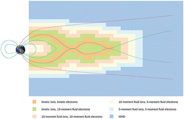
Figure 1. Oversimplified sketch of a multiphysics approach for tail reconnection.
With this multiphysics strategy, these codes can be applied to problem sizes that are otherwise impossible to reach with kinetic simulations and the understanding of the impact of small scale phenomena on the dynamics on global scales is in reach.
The outline of the paper is as follows: first we briefly describe all the plasma models and the necessary numerical schemes (Vlasov equation, 10- and 5-moment fluid equations, Maxwell's equations, the coupling procedure, the Landau fluid closure). We will then study the Geospace Environmental Modeling (GEM) reconnection setup [24] and perform comparisons to pure kinetic and pure fluid simulations.
2. Plasma Models
The plasma models that we have to consider are: (i) the Vlasov equation, (ii) Maxwell's equations, and (iii) the 10- and 5-moment fluid equations. We will briefly summarize these sets of equations.
2.1. Vlasov Equation
Collisionless plasmas on the finest level of description are governed by the Vlasov equation
where denotes the phase-space density, qs and ms the particle charge and mass for species s ∈ {e, i} (electrons and ions). The electric and magnetic fields and are given by Maxwell's equations:
with speed of light c and electric constant ε0. Maxwell's equations depend on charge and current densities ρ and , which are obtained from the phase-space densities :
Vlasov equation (1) and Maxwell's equations (2) form a closed set of equations and constitute the most fundamental description of a collisionless plasma.
2.2. Two-Species Fluid Equations
Fluid descriptions can be obtained from the Vlasov Equation (1) by taking moments of the phase-space density fs,
Here, denotes the n-fold tensor product of with itself, . Typically, only the first few moments are considered since a Gaussian distribution is exactly represented by the moments μ0,s, μ1,s, μ2,s (and all other moments equaling zero).
We will subsequently describe the 10- and 5-moment equations. Consider the lowest moments up to μ3,s :
ns, , 𝔼s are evolved by the following equations, obtained from the Vlasov Equation (1):
where sym(·) symmetrizes its argument. Naturally, these equations are not closed. Designing appropriate fluid closures have a long history. An excellent overview is given in Chust and Belmont [8]. In order to mimic kinetic Landau damping effects, several closures have been developed (see [5, 6]), all based on the early Hammett and Perkins model [4].
Wang et al. [1] suggested a heat flux closure which approximates a spectrum of wave numbers by one single wave number k0. Following this idea, Allmann-Rahn et al. [3] developed an improved model that is able to correctly describe the kinetic scaling of average reconnection rate as a function of the distance between the islands' O-points λ and where di denotes the ion skin depth (see Figure 9 in [3]).
In the simulations used in this paper the original k0-closure from Wang et al. [1] is used. It approximates the divergence of the heat flux with an expression that forces an anisotropic pressure tensor to a more isotropic one. More precisely, the expression reads
with the pressure tensor , the scalar pressure and thermal velocity vth. The parameter k0 is choosen on the order of the inverse Debye length. Together with (6), this constitutes a closed set of ten fluid equations.
In future simulations it is planed to switch to the improved model introduced in Allmann-Rahn et al. [3].
As an alternative to the 10-moment description, an even simpler 5-moment description can be introduced where the energy density tensor and heatflux tensor are replaced by the scalar energy density and vector heat flux . The scalar energy density evolves in time according to:
Together with the assumption of adiabaticity, , (6a, 6b, 8) form the set of five moment equations.
Completely analogous to the case of the Vlasov equation, the source terms ρ and j in Maxwell's Equations (2) are formed from the particle densities ns (see Equation (5a)). Actually, as will be described in section 3.3, only the current density j is needed to propagate Maxwell's equations.
3. Numerical Methods
3.1. Vlasov Equation
In order to circumvent the complexity that could arise from the high dimensionality of the phase space, the Vlasov equation is split into five one-dimensional problems using Strang splitting [25]. These one-dimensional advection problems are solved with a third order semi-Lagrangian flux-conservative scheme introduced by [26]. Thus the scheme conserves density but not energy. Work on conservation of momentum and energy is in progress (see [27]) but not yet fully implemented in our multiphysics framework.
In order to minimize the error due to the Strang splitting when calculating the backward characteristics needed in the semi-Lagrangian method, the cascade interpolation [28] is combined with the Boris step [29] to form the backsubstitution method introduced in Schmitz and Grauer [30]. Details of this procedure can be found in Schmitz and Grauer [31].
The code is fully parallelized using the message passing interface (MPI) [32] where the Vlasov part is solved in parallel on distributed graphics cards using CUDA programming tools [33].
3.2. Two-Species Fluid Equations
Both the 10-moment and the 5-moment two-species fluid models are all discretized with the same numerical methods.
For the discretization in space, we use the CWENO scheme introduced by Kurganov and Levy [34], an easy to implement third order finite-volume scheme which is a perfect compromise between sharp shock resolution and high-order approximation in spatially smooth regions. A third order strong-stability-preserving Runge-Kutta scheme [35] is employed for the time integration.
3.3. Maxwell's Equation
The electromagnetic fields are positioned on a staggered Yee grid [36] in order to maintain the divergence free condition for the magnetic field: ∇ · B = 0. Equations (2c, 2d) are evolved through the FDTD method presented in Taflove and Brodwin [37]. Here, only the current density j enters as a source term. Since the speed of light exceeds all other speeds found in the plasma by far, subcycling is used in order to resolve lightwaves while keeping the global timestep as large as possible. In addition, the speed of light is artificially reduced to 20 times the Alfvén speed.
3.4. Adaptive Coupling
The coupling strategy is the most important and at the same time the most critical part of the multiphysics simulations. The coupling strategy involves two separate problems: first, providing the correct boundary conditions at interfaces between different physical models and second, designing criteria to decide which model can be used in which part of the computational domain in an adaptive way.
We start with discussing the strategy for obtaining boundary conditions at the interfaces. Providing boundary conditions for the fluid part at the kinetic/fluid interface is rather straightforward: the fluid boundary conditions are obtained by taking the necessary moments of the phase-space densities fs at the interface. Providing boundary conditions for the phase-space densities fs from the fluid description is far less trivial and described in detail in Rieke et al. [20]. In short the procedure can be summarized as follows: we first extrapolate the phase-space density fs to the boundary region. Next, we adjust the extrapolated phase-space density fs such that the moments equal the moments from the 10-moment fluid description. In this way, we only manipulate the phase-space density fs rather “smoothly” with minimal changes and do not force fs to a Gaussian shape. The coupling between the 10-moment and 5-moment fluid regions is done in a very natural way. The boundary conditions for the 5-moment description is simply obtained by calculating the energy scalar from the trace of the energy density tensor. In the other direction, the energy tensor has to be constructed from the energy scalar by assuming a diagonal shape at the 10-/5-moment interface.
The criteria to decide which of the available models shall be used in which subregion of the domain is a highly non-trivial issue. Presently, our strategy is still in a phase of proof of concept and further work has to be invested. For the case of magnetic reconnection, we implemented heuristic criteria based on the current density jz since it is a good indicator for regions of high reconnection. In order to allow for a finer detachment of electrons and ions, we actually use the velocity uz, s = nsûz, s for electrons and ions separately. This is reasonable as the current density is given by (compare (3b)). We note that the same criterium is used to introduce a finer level of description (e.g. changing a 10 moment fluid region into a Vlasov region) as well as “coarsening” the physical model (e.g. changing a Vlasov region into a fluid region). Also note that we do not introduce overlap regions or buffer zones. It should be stated clearly that a criterion based on the current density is rather heuristic and far from universally applicable approach and further work has to be invested on robust criteria.
In addition, once a criterion is considered satisfactory for the context, thresholds have to be defined that mirror a good trade-off between the need to use a higher-information model for a correct representation and the opportunity to save computational resources with a lower-information model. Up to know we can only state that this is based on educated guesses.
3.5. Code Performance
The described numerical codes, the adaptive coupling procedures and the parallelization framework based on space-filling curves [38] is build in our framework called muphy. This framework has been developed over the last 10 years. It is written in C++/CUDA, runs partly on GPUs and partly on CPUs and employs MPI for parallelization.
Scaling runs have been performed on the JURECA supercomputer at the FZ Jülich, Germany [39], on a fully kinetic Whistler-wave setting [18]. Scaling results are excellent as shown in Table 1 and Figure 2. Note that the number of GPUs was only restricted by the actual configuration of JURECA.
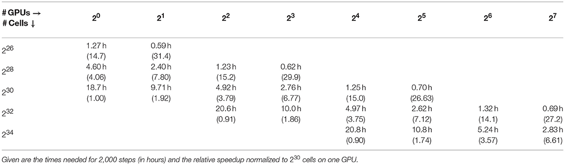
Table 1. Scaling behavior of muphy on JURECA across different problem sizes (absolute number of grid cells) and number of GPUs.
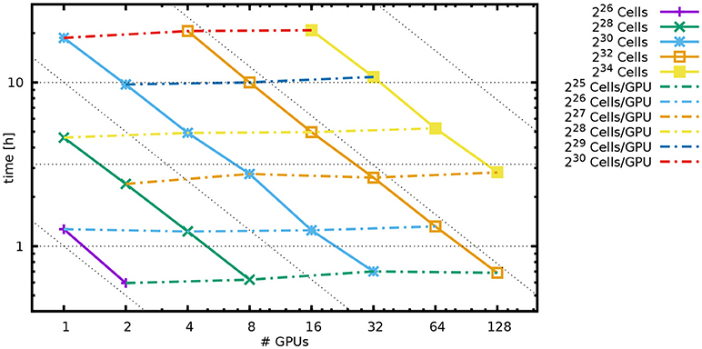
Figure 2. Scaling behavior of muphy on JURECA. Same data as in Table 1.
4. Results
We apply the described models and the multiphysics coupling strategy to the Geospace Environmental Modeling (GEM) Magnetic Reconnection Challenge [24], which has been set up to study 2d reconnection. It is a Harris sheet equilibrium with magnetic field
density
magnetic flux perturbation
initially uniform electron and ion temperatures of ratio Ti/Te = 5, and mass ratio mi/me = 25. Moreover, B0 = 1, n0 = 1, ψ0 = 0.1, λ = 0.5 in the standard normalized units. While the original domain size is Lx = 25.6di, Ly = 12.8di, we use the slightly smaller Lx = 8πdi, Ly = 4πdi with ion inertial length di, as we have depicted in Table 2. The symmetry properties of the GEM problem make it sufficient to calculate only one quarter of the spatial domain. We use a uniform cell-width of dx = d in 2d physical space and a uniform resolution of 32 cells in each direction in 3d velocity space. To reduce the computational costs, we use the reduced speed of light of 20 times the Alfvén speed. The numerical setup is depicted in Table 2.
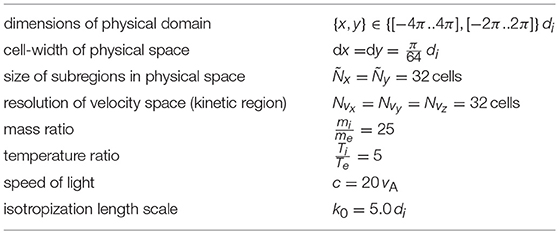
Table 2. Numerical setup of GEM.
In the simulation we use the uz,s-based criterion with a thresholds depicted in Table 3. The criterion is reassessed every (inverse ion-gyrofrequencies) for every subregion.
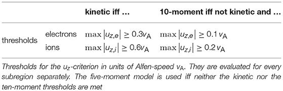
Table 3. Numerical setup of GEM.
In Figure 3 the fields jz, uz,e and uz,i are shown together with the areas depicting the different physical models for different times of the simulation. From these figures one can deduce that substantial saving in simulation time can be achieved since the performance gain is approximately proportional to the ratio of the computational domain to the area where the Vlasov equation is solved. A video showing the dynamical evolution depicted in Figure 3 is available in the Supplementary Material section.
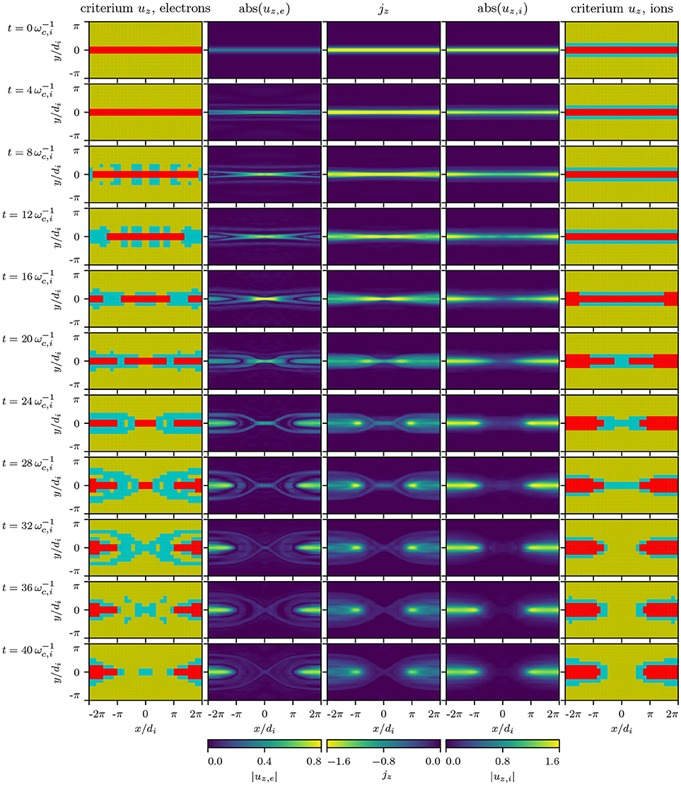
Figure 3. |uz,e|, jz and |uz,i| for different times in units of inverse ion-gyrofrequencies . On the outsides, the preferred models are depicted based on the values of uz,s and threshold as given in Table 3. Red areas are solved with the kinetic solver, blue areas with the ten-moment and yellow areas with the five-moment fluid solver. Note that the initial spacial distribution of models at time t = 0 have been prescribed.
In Figure 4, a comparison of different simulations are shown and compared to the multiphysics run. Depicted is the current density jz at the time of the highest reconnection rate. The fully kinetic Vlasov simulation agrees rather well with the multiphysics simulation. The overall agreement is substantially better than the results obtained from the 10- and 5-moment simulations. However, differences especially in the precise values of the absolute maxima of the current density, are visible. Whether this is an effect of the model selection criteria has to be tested in further investigations.
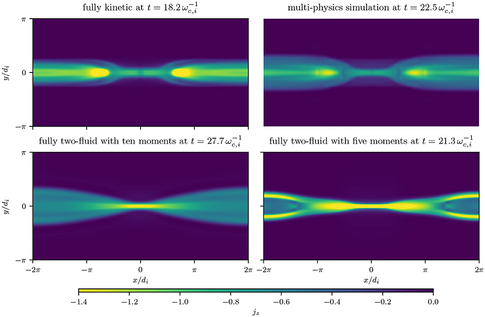
Figure 4. jz at highest reconnection rate for the coupled run and some uncoupled comparison runs with a single solver.
As a more quantitative comparison, the reconnecting flux for the multiphysics simulation is plotted in Figure 5 together with purely kinetic and fluid runs. There are a number of things to observe from the plot: While the reconnecting flux of the fluid runs does not saturate within the simulation time, the kinetic and the multiphysics runs saturate. In addition, they both saturate at the same level and thus capture essentially the same small scale physics which is not possible with the fluid models.
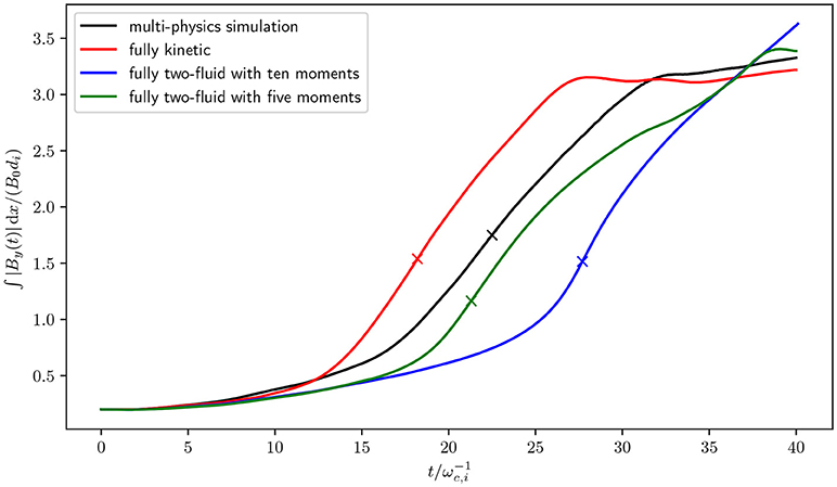
Figure 5. Reconnection fluxes for the coupled run and some uncoupled comparison runs with a single solver. Crosses mark the point of highest reconnection rate throughout the respective run.
Alone the presence of electron and ion kinetic regions in the very center of reconnection zone and 10-moment fluid regions around it seems to ensure the characteristic behavior of the full kinetic reconnection scenario.
5. Discussion
We showed that the proposed multiphysics coupling hierarchy can give excellent results even when only a small part of computational domain near the reconnection zone is captured with a kinetic model.
However, still many questions and challenges remain and it is clear that the present simulations are only on the level of a proof of concept. Most important is the issue of designing robust physics refinement criteria and their thresholds. First attempts based on the heat flux are under investigation. In addition, the multiphysics coupling strategy should be formulated as an asymptotic preserving scheme [40, 41]. The coupling of the 10- and 5-moment models is already in this state when incorporating the effect of Landau damping [1, 3]. Presently, we are also reformulating the coupling between the Vlasov and the 10-moment model. For this, we formulate the kinetic description as an adaptive (in time and space) δf method and ease the transition to the fluid description as an asymptotic preserving scheme. Finally, the multiphysics hierarchy should not stop at the level of the 5-moment fluid description. Work to couple the 5-moment model to MHD is in progress.
Data Availabilty Statement
The datasets generated for this study can be found on the data server https://vlasov.tp1.ruhr-uni-bochum.de/data/paper-frontiers-2018.
Author Contributions
All authors listed have made a substantial, direct and intellectual contribution to the work, and approved it for publication.
Conflict of Interest Statement
The authors declare that the research was conducted in the absence of any commercial or financial relationships that could be construed as a potential conflict of interest.
Acknowledgments
We acknowledge interesting discussions with F. Allmann-Rahn, J. Dreher and T. Trost. Computations were conducted on the Davinci cluster at TP1 Plasma Research Department and on the JURECA cluster at Jülich Supercomputing Center under the project number HBO43. The authors gratefully acknowledge the computing time granted by the John von Neumann Institute for Computing (NIC) and provided on the supercomputer JURECA at Jülich Supercomputing Centre (JSC).
Supplementary Material
The Supplementary Material for this article can be found online at: https://www.frontiersin.org/articles/10.3389/fphy.2018.00113/full#supplementary-material
Video S1. Dynamical evolution of |uz,e|, |uz,i| together with the refinement criteria. red: Vlasov solver, blue: 10-moment fluid solver, yellow: 5-moment fluid solver.
References
1. Wang L, Hakim AH, Bhattacharjee A, Germaschewski K. Comparison of multi-fluid moment models with particle-in-cell simulations of collisionless magnetic reconnection. Phys Plasmas (2015) 22:012108. doi: 10.1063/1.4906063
2. Ng J, Hakim A, Bhattacharjee A, Stanier A, Daughton W. Simulations of anti-parallel reconnection using a nonlocal heat flux closure. Phys Plasmas (2017) 24:082112. doi: 10.1063/1.4993195
3. Allmann-Rahn F, Trost T, Grauer R. Temperature gradient driven heat flux closure in fluid simulations of collisionless reconnection. J Plasma Phys. (2018). doi: 10.1017/S002237781800048X
4. Hammett GW, Perkins FW. Fluid moment models for Landau damping with application to the ion-temperature-gradient instability. Phys Rev Lett. (1990) 64:3019–22. doi: 10.1103/PhysRevLett.64.3019
5. Hammett GW, Dorland W, Perkins FW. Fluid models of phase mixing, Landau damping, and nonlinear gyrokinetic dynamics. Phys Fluids B. (1992) 4:2052–61. doi: 10.1063/1.860014
6. Passot T, Sulem PL. Long-Alfvén-wave trains in collisionless plasmas. II. A Landau-fluid approach. Phys Plasmas. (2003) 10:3906–13. doi: 10.1063/1.1600442
7. Sharma P, Hammett GW, Quataert E. Transition from collisionless to collisional magnetorotational instability. Astrophys J. (2003) 596:1121. doi: 10.1086/378234
8. Chust T, Belmont G. Closure of fluid equations in collisionless magnetoplasmas. Phys Plasmas. (2006) 13:012506. doi: 10.1063/1.2138568
9. Schulze TP, Smereka PEW. Coupling kinetic Monte-Carlo and continuum models with application to epitaxial growth. J Comput Phys. (2003) 189:197–211. doi: 10.1016/S0021-9991(03)00208-0
10. Degond P, Dimarce G, Mieussens L. A multiscale kinetic-fluid solver with dynamic localization of kinetic effects. J Comput Phys. (2010) 229:4907–33. doi: 10.1016/j.jcp.2010.03.009
11. Dellacherie S. Kinetic-fluid coupling in the field of the atomic vapor isotopic separation: numerical results in the case of a monospecies perfect gas. AIP Conf Proc. (2003) 663:947–56. doi: 10.1063/1.1581642
12. Goudon T, Jin S, Liu JG, Yan B. Asymptotic-preserving schemes for kinetic-fluid modeling of disperse two-phase flows. J Comput Phys. (2013) 246:145–64. doi: 10.1016/j.jcp.2013.03.038
13. Tiwari S, Klar A. An adaptive domain decomposition procedure for Boltzmann and Euler equations. J Comput Appl Math. (1998) 90:223–37. doi: 10.1016/S0377-0427(98)00027-2
14. Le Tallec P, Mallinger F. Coupling Boltzmann and Navier-Stokes Equations by Half Fluxes. J Computational Physics. (1997) 136:51–67. doi: 10.1006/jcph.1997.5729
15. Sugiyama T, Kusano K, Hirose S, Kageyama A. MHD–PIC Connection Model in a Magnetosphere–ionosphere Coupling System. J Plasma Phys. (2006) 72:945–8. doi: 10.1017/S0022377806005356
16. Sugiyama T, Kusano K. Multi-scale plasma simulation by the interlocking of magnetohydrodynamic model and particle-in-cell kinetic model. J Comput Phys. (2007) 227:1340–52. doi: 10.1016/j.jcp.2007.09.011
17. Markidis S, Henri P, Lapenta G, Rönnmark K, Hamrin M, Meliani Z, et al. The fluid-kinetic particle-in-cell method for plasma simulations. J Comput Phys. (2014) 271:415–29. doi: 10.1016/j.jcp.2014.02.002
18. Daldorff LKS, Tóth G, Gombosi TI, Lapenta G, Amaya J, Markidis S, et al. Two-way coupling of a global Hall magnetohydrodynamics model with a local implicit particle-in-cell model. J Comput Phys. (2014) 268:236–54. doi: 10.1016/j.jcp.2014.03.009
19. Kolobov VI, Arslanbekov RR. Towards adaptive kinetic-fluid simulations of weakly ionized plasmas. J Comput Phys. (2012) 231:839–69. doi: 10.1016/j.jcp.2011.05.036
20. Rieke M, Trost T, Grauer R. Coupled vlasov and two-fluid codes on GPUs. J Comput Phys. (2015) 283:436–52. doi: 10.1016/j.jcp.2014.12.016
21. Tóth Gábor, Jia Xianzhe, Markidis Stefano, Peng Ivy Bo, Chen Yuxi, Daldorff Lars K S, et al. Extended magnetohydrodynamics with embedded particle-in-cell simulation of Ganymede's magnetosphere. J Geophys Res. (2016) 121:1273–93. doi: 10.1002/2015JA021997
22. Tóth G, Chen Y, Gombosi TI, Cassak P, Markidis S, Peng IB. Scaling the ion inertial length and its implications for modeling reconnection in lobal simulations. J Geophys Res. (2017) 122:10336–55. doi: 10.1002/2017JA024189
23. Makwana KD, Keppens R, Lapenta G. Two-way coupling of magnetohydrodynamic simulations with embedded particle-in-cell simulations. Comput Phys Commun. (2017) 221:81–94. doi: 10.1016/j.cpc.2017.08.003
24. Birn J, Drake JF, Shay MA. Geospace Environmental Modeling (GEM) magnetic reconnection challenge. J Geophys Res. (2001) 106:3715–9. doi: 10.1029/1999JA900449
25. Strang G. On the construction and comparison of difference schemes. SIAM J Numer Anal. (1968) 5:506–17. doi: 10.1137/0705041
26. Filbet F, Sonnendrücker E, Bertrand P. Conservative numerical schemes for the Vlasov equation. J Comput Phys. (2001) 172:166–87. doi: 10.1006/jcph.2001.6818
27. Trost T, Lautenbach S, Grauer R. Enhanced conservation properties of Vlasov codes through coupling with conservative fluid models. ArXiv e-prints. (2017).
28. Leslie LM, Purser RJ. Three-dimensional mass-conserving semi-Lagrangian scheme employing forward trajectories. Month Weather Rev. (1995) 123:2551–66. doi: 10.1175/1520-0493(1995)123<2551:TDMCSL>2.0.CO;2
29. Boris JP. Relativistic plasma simulation-optimization of a hybrid code, in Proceedings of the Conference on the Numerical Simulation of Plasmas. Washington DC: U.S. Naval Research Laboratory (1970). 3–67.
30. Schmitz H, Grauer R. Darwin-Vlasov simulations of magnetised plasmas. J Comput Phys. (2006) 214:738–56. doi: 10.1016/j.jcp.2005.10.013
31. Schmitz H, Grauer R. Comparison of time splitting and backsubstitution methods for integrating Vlasov's equation with magnetic fields. Comp Phys Commun. (2006) 175:86–92. doi: 10.1016/j.cpc.2006.02.007
33. nVidia corp. nVidia CUDA C Programming Guide (2013). Available online at: http://docs.nvidia.com/cuda/cuda-c-programming-guide/index.html
34. Kurganov A, Levy D. A third-order semidiscrete central scheme for conservation laws and convection-diffusion equations. SIAM J Sci Comput. (2000) 22:1461–88. doi: 10.1137/S1064827599360236
35. Shu CW, Osher S. Efficient implementation of essentially non-oscillatory shock-capturing schemes. J Comput Phys. (1988) 77:439–71. doi: 10.1016/0021-9991(88)90177-5
36. Yee KS. Numerical solution of initial boundary value problems involving Maxwell's equations in isotropic media. IEEE Trans Antennas Propag. (1966) 14:302–7. doi: 10.1109/TAP.1966.1138693
37. Taflove A. Computational electrodynamics: the finite-difference time-domain method. Norwood, MA: Artech House (1995).
38. Dreher J, Grauer R. racoon: a parallel mesh-adaptive framework for hyperbolic conservation laws. Parallel Comput. (2005) 31:913. doi: 10.1016/j.parco.2005.04.011
39. Jülich Supercomputing Centre. JURECA: general-purpose supercomputer at Jülich supercomputing centre. J Large Scale Res Facilit. (2016) 2:1–7. doi: 10.17815/jlsrf-2-121
40. Degond P, Deluzet F. Asymptotic-preserving methods and multiscale models for plasma physics. J Comput Phys. (2017) 336:429–57. doi: 10.1016/j.jcp.2017.02.009
41. Hu J, Jin S, Li Q. Chapter 5 - asymptotic-preserving schemes for multiscale hyperbolic and kinetic equations. In: Abgrall R, Shu CW editors. Handbook of Numerical Methods for Hyperbolic Problems. Vol. 18 of Handbook of Numerical Analysis. Elsevier (2017). 103–29. Available online at: http://www.sciencedirect.com/science/article/pii/S1570865916300102
Keywords: multiphysics coupling, kinetic plasmas, fluid descriptions, numerical simulations, reconnection
Citation: Lautenbach S and Grauer R (2018) Multiphysics Simulations of Collisionless Plasmas. Front. Phys. 6:113. doi: 10.3389/fphy.2018.00113
Received: 14 May 2018; Accepted: 11 September 2018;
Published: 08 October 2018.
Edited by:
Vladimir I. Kolobov, CFD Research Corporation, United StatesReviewed by:
Ammar H. Hakim, Princeton University, United StatesGiovanni Lapenta, KU Leuven, Belgium
Copyright © 2018 Lautenbach and Grauer. This is an open-access article distributed under the terms of the Creative Commons Attribution License (CC BY). The use, distribution or reproduction in other forums is permitted, provided the original author(s) and the copyright owner(s) are credited and that the original publication in this journal is cited, in accordance with accepted academic practice. No use, distribution or reproduction is permitted which does not comply with these terms.
*Correspondence: Rainer Grauer, grauer@tp1.rub.de