Efficient Criteria of Quantumness for a Large System of Qubits

1 Introduction

One of the key obstacles in the way to the full development of quantum technologies 2.0 [1] is the same circumstance which stimulated their development in the first place: the fundamental impossibility of an efficient simulation of a large enough, quantum coherent structure with classical means. In practice “large enough” turned out to be a system comprising a hundred or so quantum bits, which is still too small to form a quantum computer capable of simulating other “large enough” quantum systems. On the other hand, artificial quantum coherent systems comprising thousands of qubits are being fabricated [2] and even successfully used, like commercial quantum annealers [3, 4]. Arrays of superconducting qubits are also being considered as microwave range detectors capable of exceeding the standard quantum limit (in such application as, e.g., search for galactic axions [5]). Quantum coherence of the array is the key element of the detection mechanism. This “quantum capacity gap” [6] needs to be bridged, in order to allow a systematic progress towards the development of the full potential of quantum technologies 2.0, such as noisy intermediate-scale quantum (NISQ) devices [7] and universal fault tolerant quantum computers.

The impossibility of an efficient classical simulation of a large quantum system is not absolute, in the sense that it concerns the simulation of an arbitrary evolution of such a system, whereby its state vector can reach all of its (exponentially high-dimensional) Hilbert space and has potentially infinite time to do so. The Margolus-Levitin theorem and its generalizations [8–13] put a limit on the speed of such evolution, thus restricting the accessible part of the Hilbert space for any finite time interval. This agrees with a proof [14] that the manifold of all quantum many-body states that can be generated by arbitrary time-dependent local Hamiltonians in a time that scales polynomially in the system size occupies an exponentially small volume in its Hilbert space. (This is a literally correct statement, since the Hilbert space of a system of qubits is a finite-dimensional complex projective space; that is, it is compact and, moreover, it has a unitary invariant Fubini-Study metric [15]). Numerical and analytical studies also indicate that the number of independent constraints describing quantum evolution may be much less than the dimensionality of the Hilbert space [16]. It is therefore reasonable to suggest that a “general case” evolution of a large quantum coherent quantum structure can be characterized by a non-exponentially large set of dimensionless parameters, which correspond to qualitatively different regimes of evolution of this structure. Our recent numerical simulations indicate the existence of such regimes in a set of qubits with pumping and dissipation [17].

Such dimensionless parameters, if exist, will be combinations of fundamental physical constants and parameters, which characterize the system. (We will only need the Planck constant, since the speed of light and gravity constant are not relevant for the currently feasible devices). For example, in the standard approximation, a system of qubits is described by a quantum Ising Hamiltonian,

$\widehat{H}(t)=\sum _{i\ne j}{J}_{ij}(t){\sigma }_i^z{\sigma }_j^z-\frac{1}{2}\sum _j\left(h_j(t){\sigma }_j^z+{\mathrm{\Delta }}_j(t){\sigma }_j^x\right),(1)$

and a set of Lindblad operators responsible for dephasing and relaxation of separate qubits, with characteristic times, respectively, t_ϕ and t_r, and their combination, the decoherence time t_D. In the case of an adiabatic quantum processor [3, 4], the time dependence of the Hamiltonian parameters J_ij, h_j and Δ_j (except that induced by the ambient noise) is determined by that of the adiabatic parameter λ (t) (in the simplest case, by the time of adiabatic evolution, t_f). Then, the dimensionless characteristics of the system should be the combinations of ℏ with the following quantities:

(1) Dimensionless: N (number of qubits); ⟨z⟩ (connectivity of the network: average number of couplings per qubit); ⟨δz²⟩ (its dispersion); ⟨z_iz_j⟩ (its correlation function); …;

(2) Powers of energy: ⟨E⟩ (average qubit excitation energy); ⟨δE²⟩; ⟨E_iE_j⟩; ⟨J⟩ (average coupling strength); ⟨δJ²⟩; ⟨J_iJ_k⟩; k_BT; …;

(3) Powers of time: t_ϕ; t_r; t_D; t_f; $\dot{\lambda }\sim 1/t_f$ (speed of evolution); $\ddot{\lambda }$; …;

and such additional parameters as, e.g., the spectral density of ambient noise S_A (f). Note that all these parameters can be efficiently obtained by either direct measurements or straightforward calculations.

The field of several dozens of independent dimensionless combinations of the above parameters is narrowed for a particular quantum system and the mode of its operation. Here we concentrate on adiabatic quantum computing (quantum annealing). The Hamiltonian of a quantum system is here manipulated in such a way that its ground state changes from the easily accessible one to the one encoding a solution to the desired problem (and presumably having a very complex structure, so that reaching it by annealing would be improbable). In the case of a slow enough evolution of the Hamiltonian H (t), the system initialized in the ground state of H (0) will evolve into the ground state of H (t_f) by virtue of the adiabatic theorem [18]. If the system is totally insulated, the quantum speed and accessibility theorems [8–14] do not put fundamental constraints on an adiabatic quantum computer. Nevertheless, in a realistic case, the computation time is limited by interactions with the outside world leading to nonunitarity [19], and the question arises whether the evolution from the initial to the desired final state of the system is possible. As we see, the question of accessibility of different regions of the Hilbert space is especially relevant in this case.

An intriguing twist is added by the fact that the operation of D-Wave processors demonstrated what looked convincingly like quantum annealing [20, 21] despite the large discrepancy between the adiabatic evolution time, t_f (microseconds [20]), and the qubit decoherence time, t_D ≪ t_f (tens of nanoseconds [22]), in the absence of any quantum error correction. On the second thought, it is not so surprising. The quantum state of an adiabatic quantum computer evolves starting at t = 0 from a factorized state, |in⟩. The computation is successful, if at the time t = t_f there is a sufficient ratio of quantum trajectories ending in the state |out⟩, which is also factorized by design. Decoherence tends to disrupt quantum correlations between different qubits, and thus constrain the trajectories to partially factorized submanifolds of the Hilbert space. Nevertheless the success does not necessarily require that these trajectories pass through globally entangled states, and thus certain degree of decoherence may not necessarily make the proper operation of the device impossible.

While it cannot be predicted whether the evolution of a given quantum system can take it from the given initial to the desired final state, the average of the maximal distance between some initial and some final state of the system, for given values of t_f and other system parameters, may serve as a heuristic indicator of success. This distance can be naturally determined via the Fubini-Study metric [15], in which the distance s (ϕ, ψ) between states |ϕ⟩ and |ψ⟩ is given by

$\cos s(\varphi ,\psi )=\sqrt{\frac{\langle \varphi |\psi \rangle \langle \psi |\varphi \rangle }{\langle \varphi |\varphi \rangle \langle \psi |\psi \rangle }}.(2)$

The maximal Fubini-Study distance in the Hilbert space is π/2, the distance between mutually orthogonal states. We will therefore choose the quantity

$\mathcal{S}=\frac{2}{\pi }\sqrt{\overline{s^2(\varphi ,\psi )}}(3)$

as an ad hoc parameter, which characterizes the ability of an adiabatically evolving quantum device to reach its desired quantum state. The bar denotes the averaging over all initial states and over all quantum trajectories accessible to the system, which connect them to the final states maximally removed from them (in terms of the Fubini-Study distance).

2 Random Walk Model: Heuristic Treatment

The evolution of the state vector of a quantum system can be modeled by a series of random collapses to one of its instantaneous eigenstates at the moments t₁, t₂, …, and unitary evolutions under the Hamiltonian $\widehat{H}(t)$ between these moments. In the limit of infinitesimally small time intervals between subsequent collapses, this picture leads to the Quantum State Diffusion approach (QSD). Averaging over individual QSD trajectories reproduces the standard quantum master equation for the density matrix and provides an efficient basis for numerical calculation [23].

For our purpose it is essential to keep the decoherence time as an explicit parameter. Therefore, the model we use is a random walk in the Hilbert space of the system, with the step (Fubini-Study) lengths Δs_j dependent on Δt. For small time intervals of unitary evolution $|\varphi \rangle =e^{-i\widehat{H}\mathrm{\Delta }t}|\psi \rangle$, the distance s (ϕ, ψ) is given by (see Supplementary Appendix SA).

$s\approx \frac{\mathrm{\Delta }t}{\hslash }{\sigma }_{\widehat{H}}(\psi ).(4)$

Here, ${\sigma }_{\widehat{H}}^2(\psi )\equiv {⟨{\widehat{H}}^2⟩}_{\psi }-{⟨\widehat{H}⟩}_{\psi }^2$ is the energy dispersion during the unitary evolution, where ⟨⋅⟩_ψ is the expectation value for a quantum state |ψ⟩, i.e., ⟨⋅⟩_ψ ≡⟨ψ|⋅|ψ⟩. This expression is intuitively plausible: energy and time are the only parameters in the problem, and in case of zero energy variance the system would be in an eigenstate of the Hamiltonian and remain in it, barring degeneracies. The energy variance is made possible by the interaction with the environment, which is implicit in the assumption of random collapses of the quantum state of the system.

Substituting here the maximal possible value of s = π/2, we find

$\mathrm{\Delta }{t}_{\text{max}}=\frac{\pi }{2}\frac{\hslash }{{\sigma }_{\widehat{H}}(\psi )}.(5)$

This coincides with the rigorous Mandelstam-Tamm expression for the minimal time necessary to evolve from an initial state to a state orthogonal to it [8].

Now consider the random walk of M ≫ 1 steps of identical duration Δt, controlled by independently distributed random Hamiltonians ${\widehat{H}}_j(j=\mathrm{1,2},\dots M)$ (but still assuming that the total displacement remains small). Using the same approximation as before, the span of this random walk (i.e., the Fubini-Study distance between its initial point |ψ⟩ and final point $|\varphi \rangle ={\prod }_j\exp (-i\mathrm{\Delta }t{\widehat{H}}_j/\hslash )|\psi \rangle$) is thus found directly (see Supplementary Appendix SB):

$s(\varphi ,\psi )\approx \frac{\mathrm{\Delta }t}{\hslash }{\sigma }_{\sum _j{\widehat{H}}_j}(\psi ),(6)$

where,

$\begin{array}{ll}\hfill {\sigma }_{\sum _j{\widehat{H}}_j}(\psi )=& {\langle \sum _j{\widehat{H}}_{j}2\rangle }_{\psi }-{\langle \sum _j{\widehat{H}}_j\rangle }_{\psi }^2\hfill \end{array}(7)$

$\begin{array}{ll}\hfill =& \sum _{\chi \ne \psi }\sum _{jk}⟨\psi |{\widehat{H}}_j|\chi ⟩⟨\chi |{\widehat{H}}_k|\psi ⟩.\hfill \end{array}(8)$

Here the summation is taken over the states |χ⟩ from the orthonormal basis of the Hilbert space of our system, which includes the state |ψ⟩.

Making a further simplification, assume that all random steps have the same length $\mathrm{\Delta }S=\overline{{\sigma }_{\widehat{H}}}\mathrm{\Delta }t/\hslash$. Then the r.m.s. of the span is

$\sqrt{\overline{s{(\varphi ,\psi )}^2}}\approx \mathrm{\Delta }S\frac{\sqrt{\stackrel{̄}{{\sigma }_{\sum _j{\widehat{H}}_j}^2(\psi )}}}{\overline{{\sigma }_{\widehat{H}}(\psi )}},(9)$

where the bar average is over random choice of H_j-Hamiltonians and initial states |ψ⟩.

After averaging over random Hamiltonians ${\widehat{H}}_j$ and states |ψ⟩, which gives $\overline{{\sum }_j⟨\psi |{\widehat{H}}_j|\chi ⟩}\approx 0$, the only term surviving will be $\stackrel{̄}{{\sigma }_{\sum {\widehat{H}}_j}^2(\psi )}={\sum }_{\chi \ne \psi }{\sum }_j\overline{|⟨\psi |{\widehat{H}}_j|\chi ⟩{|}^2}$. We thus have

$\begin{array}{ll}\hfill \stackrel{̄}{{\sigma }_{\sum {\widehat{H}}_j}^2(\psi )}=& \sum _{j=1}^M\sum _{\chi \ne \psi }\overline{|⟨\psi |{\widehat{H}}_j|\chi ⟩{|}^2}\hfill \end{array}(10)$

$\begin{array}{ll}\hfill \approx & Mf(N){\overline{{\sigma }_{\widehat{H}}(\psi )}}^2.\hfill \end{array}(11)$

Here, f(N) is some function of the dimension of the Hilbert space D = 2^N, which is given by ${\sum }_{\chi \ne \psi }\overline{|⟨\psi |{\widehat{H}}_j|\chi ⟩{|}^2}\equiv f(N){\overline{{\sigma }_{\widehat{H}}(\mathrm{\Psi })}}^2$, where we used the fact that the averaged value with respect to the random ${\widehat{H}}_j$ is j-independent.

Then we obtain from Eq. 3

$\mathcal{S}\approx \frac{2}{\pi }\mathrm{\Delta }S{M}^{1/2}f{(N)}^{1/2}.(12)$

In particular, the condition $\mathcal{S}=1$ yields the relation between M and ΔS, for which the random walk is likely to connect mutually orthogonal states in the Hilbert space (a maximal random walk), and thus the quantum adiabatic operation of the system we model should be possible. This “critical value” of ΔS for a given M, N is

$\mathrm{\Delta }S=\frac{\pi }{2}{M}^{-1/2}f{(N)}^{-1/2}.(13)$

3 Random Walk Model: Numerical Approach

The goal of our numerical simulations is to determine the function f(N) in Eq. 13 through the relation between the Fubini-Study length of a single step, ΔS, and the number of steps, M, of a maximal random walk in the D = 2^N-dimensional Hilbert space (see Figures 1A,B).

FIGURE 1

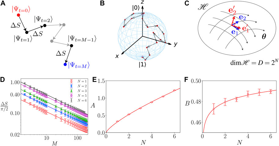
FIGURE 1. Random walk in the Hilbert space. (A) Schematics of states walking randomly in the Hilbert space. The points represent states. The state walks randomly from |Ψ_t=0⟩ to |Ψ_t=M⟩, where the stride of each step is given by the Fubini-Study distance ΔS. (B) Schematic of the random walk in the Hilbert space in the Bloch sphere. The red points indicate the states, which walks with the random direction with a fixed stride ΔS. The random walker on the Bloch sphere starts from the initial state |0⟩ at the north pole, and finally reaches the state |1⟩ at the south pole. (C) For considering the uniform random walk in the Hilbert space, we generate a random vector in the local orthogonal coordinate (spanned by the bases ${\mathbf{e}}_{\mathrm{1,2}}^{\prime }$, where ${\mathbf{e}}_1^{\prime }\cdot {\mathbf{e}}_2^{\prime }=0$, for example) from the curved parameter space θ (spanned by the bases e_1,2, where e₁ ⋅e₂ ≠ 0). (D) The critical Fubini-Study distance ΔS for the random walk in the in the Hilbert space, as a function of the number of random steps M. We consider N-qubits states. The data points are the averaged value for 500 trials. Solid lines are fitted lines with ΔS = (π/2)AM^−B. The fitting is performed for M ≥ 3. (E) The fitting factor A and (F) the fitting factor B as a function of the number of qubits N. The solid lines represent fitting functions, where we used $A={\alpha }_A{N}^{{\beta }_A}$ and $B={\alpha }_B{N}^{{\beta }_B}$ for N = 1–6.

A D-dimensional quantum state can be parameterized by 2 (D—1) real parameters $\mathit{\theta }={({\theta }_1,{\theta }_2,\dots ,{\theta }_{2(D-1)})}^{\text{T}}$, because of the presence of the overall phase factor and the normalized condition. The state can be given by

$|\mathrm{\Psi }(\mathit{\theta })\rangle =\left(\begin{array}{cc}\hfill e^{i{\theta }_D}\hfill & \cos ({\theta }_1)\hfill \\ \hfill e^{i{\theta }_{D+1}}\hfill & \sin ({\theta }_1)\cos ({\theta }_2)\hfill \\ \hfill e^{i{\theta }_{D+2}}\hfill & \sin ({\theta }_1)\sin ({\theta }_2)\cos ({\theta }_3)\hfill \\ \hfill \hfill & ⋮\hfill \\ \hfill e^{i{\theta }_{2(D-1)}}\hfill & \hfill \sin ({\theta }_1)\cdots \sin ({\theta }_{D-2})\cos ({\theta }_{D-1})\hfill \\ \hfill \hfill & \hfill \sin ({\theta }_1)\cdots \sin ({\theta }_{D-2})\sin ({\theta }_{D-1})\hfill \end{array}\right).(14)$

We consider the uniform random walk in the Hilbert space using the form Eq. 14, where each step length is fixed with the Fubini-Study distance ΔS. First, we randomly prepare an initial state |Ψ_t=0⟩ in the D-dimensional Hilbert space. The state |Ψ_t(θ)⟩ at a step t is parameterized by θ. The state at t + 1 is updated as |Ψ_t+1 (θ + dθ)⟩.

The Fubini-Study distance between these states |Ψ (θ + dθ)⟩ and |Ψ (θ)⟩ can be written as

$\mathrm{\Delta }S=s({\mathrm{\Psi }}_t(\mathit{\theta }),{\mathrm{\Psi }}_{t+1}(\mathit{\theta }+d\mathit{\theta }))=\sum _{ij}{g}_{ij}d{\theta }_{i}d{\theta }_j,(15)$

where the Fubini-Study metric is given by

$\begin{array}{ll}\hfill g_{ij}(\mathit{\theta })=& ⟨{\partial }_{{\theta }_i}\mathrm{\Psi }(\mathit{\theta })|{\partial }_{{\theta }_j}\mathrm{\Psi }(\mathit{\theta })⟩\hfill \\ \hfill & -⟨{\partial }_{{\theta }_i}\mathrm{\Psi }(\mathit{\theta })|\mathrm{\Psi }(\mathit{\theta })⟩⟨\mathrm{\Psi }(\mathit{\theta })|{\partial }_{{\theta }_j}\mathrm{\Psi }(\mathit{\theta })⟩,\hfill \end{array}(16)$

with $|{\partial }_{{\theta }_i}\mathrm{\Psi }(\mathit{\theta })\rangle \equiv \partial |\mathrm{\Psi }(\mathit{\theta })\rangle /\partial {\theta }_i$ for i, j = 1, 2, … , 2 (D − 1). We generate the parameter dθ such that the Fubini-Study distance ∑_ijg_ijdθ_idθ_j satisfies the given fixed value ΔS, and the direction of the random step is uniformly random in the local orthogonal space, where the parameters θ are given in the non-orthogonal coordinates with the curved space (See Figure 1C and Supplementary Appendix SC). Since we use the form Eq. 14, the state vector remains normalized.

The span of the random walk from t = 0 to M is then given by

$s({\mathrm{\Psi }}_0,{\mathrm{\Psi }}_M)=\arccos (⟨{\mathrm{\Psi }}_0|{\mathrm{\Psi }}_M⟩).(17)$

In our simulations we fix the number of steps M and search for such a value of ΔS (“critial value”) that the final state |Ψ_t=M⟩ satisfies the condition |π/2—s (Ψ₀, Ψ_M)| ≤ ϵ for some small ϵ.

Figure 1D shows the critical value of ΔS as a function of M. Fitting yields

$\mathrm{\Delta }S=\frac{\pi }{2}A(N)M^{-B(N)},(18)$

where A(N) = 0.309 (8)N^0.76(2) and B(N) = 0.472 7 (8)N^0.020(1) (see Figures 1E,F). In these numerical simulations, we used $ϵ=\pi /2-{\cos }^{-1}(1/\sqrt{D})$, where $ϵ\approx 1/\sqrt{D}$ in the huge Hilbert space. We see that the critical value of ΔS scales almost as a power of M, since B(N) shows a very weak power law dependence on the number of qubits.

Comparing Eq. 13 with Eq. 18, we see that the dependence on M in our heuristic and numerical approaches is almost the same, while for the function f(N) we find f(N) ≈ 10.5 N^−3/2.

4 Accessibility Index, “Quantumness” Criterion and Comparison to Experiment

The quantities ΔS and M do not have a direct experimental significance. In our approximate treatment we can relate them instead to the decoherence time (during which the unitary evolution takes place), t_D, and the total time of adiabatic evolution, t_f, via

$M=\frac{t_f}{t_D};\mathrm{\Delta }S\le \frac{t_D}{\hslash }J,(19)$

where J is the typical coupling between qubits, so that J is a reasonable measure of the uncertainty of the N-qubit system’s energy during the adiabatic evolution (here we use the Mandelstam-Tamm expression). Then from Eq. 18 we find, that the necessary “quantumness” criterion for the adiabatic evolution is

$t_D\frac{2\pi J}{h}>\frac{\pi }{2}C{N}^{3/4}{\left(\frac{t_D}{t_f}\right)}^{1/2},(20)$

where C ≈ 0.31. Given all the approximations we have made, we can as well take C = 1. Then the “quantumness” condition can be written as

$\mathcal{A}>1,(21)$

where the accessibility index for a system of N qubits with average coupling strength J is

$\mathcal{A}\equiv 4\frac{J}{h}\frac{\sqrt{t_f{t}_D}}{N^{3/4}}.(22)$

Applying this criterion to the operation of the D-Wave processor described in Refs. [20, 22], with t_D ∼ 10 ns, t_f ∼ 5 µs, N ∼ 100 and J/h ∼ 5 GHz, we see that

$\mathcal{A}\approx 10^2\gg 1,(23)$

and the necessary “quantumness” condition was satisfied. This indicates that the results of Refs. [20, 22] are consistent with quantum annealing. From Eq. 21, we can evaluate the maximal size of a quantum processor for which the “quantumness” condition holds, other things being the same as in [20, 22]: $N_{\text{max}}\equiv {[4J/h]}^{4/3}{(t_f{t}_D)}^{2/3}\approx 7\times 10^4$.

Note that the condition $\mathcal{A}>1$ does not guarantee the successful operation of a quantum processor, i.e., it reaching the desired final state. It is rather the necessary, but not sufficient, condition of success.

5 Conclusion

We have investigated the generic behavior of a partially coherent system of qubits undergoing adiabatic evolution. Our aim was finding a convenient dimensionless parameter, which could characterize the degree of “quantumness” of our system. Basing our analysis on a random walk model of quantum evolution in the Hilbert space, we found a parameter allowing to evaluate the likelihood of a successful quantum transition between the initial and desired final states of the system. It is the accessibility index, expressed through the qubit decoherence time, time of evolution and the qubit coupling strength. Applying it to the case of 128-qubit D-Wave processors, we found that their evolution was consistent with quantum adiabatic transitions despite the qubit decoherence time being much smaller than the evolution time. An important future study is to assess the effectiveness of the accessibility index in more detail by considering a specific Hamiltonian system coupled to an environment.

Data Availability Statement

The raw data supporting the conclusion of this article will be made available by the authors, without undue reservation.

Author Contributions

AZ: posing the problem; SW and AZ: developing the methodology and performing analytical calculations; SW and MS: numerical calculations; SW, SK, and AZ: interpretation and analysis on the results. All authors made intellectual contribution to the work, contributed to writing and editing of the manuscript and approved the submitted version.

Funding

This paper is partly based on results obtained from a project, JPNP16007, commissioned by the New Energy and Industrial Technology Development Organization (NEDO), Japan. SW was supported by Nanotech CUPAL, National Institute of Advanced Industrial Science and Technology (AIST). AZ was partially supported by NDIAS Residential Fellowship and by the SUPERGALAX project which has received funding from the European Union’s Horizon 2020 research and innovation programme under grant agreement No 863313.

Conflict of Interest

The authors declare that the research was conducted in the absence of any commercial or financial relationships that could be construed as a potential conflict of interest.

Publisher’s Note

All claims expressed in this article are solely those of the authors and do not necessarily represent those of their affiliated organizations, or those of the publisher, the editors and the reviewers. Any product that may be evaluated in this article, or claim that may be made by its manufacturer, is not guaranteed or endorsed by the publisher.

Supplementary Material

The Supplementary Material for this article can be found online at: https://www.frontiersin.org/articles/10.3389/fphy.2021.773128/full#supplementary-material

References

1. Zagoskin A. A Brief Subjective Perspective on the Development of Quantum Technologies 2.0. J Phys Soc Jpn (2019) 88:061001. doi:10.7566/JPSJ.88.061001

CrossRef Full Text | Google Scholar

2. Kakuyanagi K, Matsuzaki Y, Déprez C, Toida H, Semba K, Yamaguchi H, et al. Observation of Collective Coupling between an Engineered Ensemble of Macroscopic Artificial Atoms and a Superconducting Resonator. Phys Rev Lett (2016) 117:210503. doi:10.1103/physrevlett.117.210503

PubMed Abstract | CrossRef Full Text | Google Scholar

3.D‐Wave Systems Introduction to the D-Wave Quantum Hardware (2019) company manual. https://www.dwavesys.com/tutorials/background-reading-series/introduction-d-wave-quantum-hardware.

Google Scholar

4. Bunyk PI, Hoskinson EM, Johnson MW, Tolkacheva E, Altomare F, Berkley AJ, et al. Architectural Considerations in the Design of a Superconducting Quantum Annealing Processor. IEEE Trans Appl Supercond (2014) 24:1–10. doi:10.1109/tasc.2014.2318294

CrossRef Full Text | Google Scholar

5. Navez P., Balanov A. G., Savelev S. E., Zagoskin A. M. Towards the Heisenberg Limit in Microwave Photon Detection by a Qubit Array. Phys. Rev. B (2021) 103, 064503.

CrossRef Full Text | Google Scholar

6. Zagoskin A. The Grand Challenge of Quantum Computing: Bridging the Capacity Gap. Front ICT (2014) 1:2. doi:10.3389/fict.2014.00002

CrossRef Full Text | Google Scholar

7. Preskill J. Quantum Computing in the NISQ Era and beyond. Quantum (2018) 2:79. doi:10.22331/q-2018-08-06-79

CrossRef Full Text | Google Scholar

8. Mandelstam L, Tamm I. Izv. Akad. Nauk SSSR Ser Fiz (1945) 9:122.

Google Scholar

9. Margolus N, Levitin LB. The Maximum Speed of Dynamical Evolution. Physica D: Nonlinear Phenomena (1998) 120:188–95. doi:10.1016/s0167-2789(98)00054-2

CrossRef Full Text | Google Scholar

10. Zwierz M, Pérez-Delgado CA, Kok P. Ultimate Limits to Quantum Metrology and the Meaning of the Heisenberg Limit. Phys Rev A (2012) 85:1. doi:10.1103/physreva.85.042112

CrossRef Full Text | Google Scholar

11. Deffner S, Lutz E. Energy-time Uncertainty Relation for Driven Quantum Systems. J Phys A: Math Theor (2013) 46:335302. doi:10.1088/1751-8113/46/33/335302

CrossRef Full Text | Google Scholar

12. Deffner S, Lutz E. Quantum Speed Limit for Non-markovian Dynamics. Phys Rev Lett (2013) 111:249. doi:10.1103/physrevlett.111.010402

CrossRef Full Text | Google Scholar

13. Deffner S, Campbell S. Quantum Speed Limits: from Heisenberg's Uncertainty Principle to Optimal Quantum Control. J Phys A: Math Theor (2017) 50:453001. doi:10.1088/1751-8121/aa86c6

CrossRef Full Text | Google Scholar

14. Poulin D, Qarry A, Somma R, Verstraete F. Quantum Simulation of Time-dependent Hamiltonians and the Convenient Illusion of Hilbert Space. Phys Rev Lett (2011) 106:170501. doi:10.1103/physrevlett.106.170501

PubMed Abstract | CrossRef Full Text | Google Scholar

15. Brody DC, Hughston LP. Geometric Quantum Mechanics. J Geometry Phys (2001) 38:19–53. doi:10.1016/s0393-0440(00)00052-8

CrossRef Full Text | Google Scholar

16. Rigol M, Dunjko V, Olshanii M. Thermalization and its Mechanism for Generic Isolated Quantum Systems. Nature (2008) 452:854–8. doi:10.1038/nature06838

PubMed Abstract | CrossRef Full Text | Google Scholar

17. Andreev AV, Balanov AG, Fromhold TM, Greenaway MT, Hramov AE, Li W, et al. Emergence and Control of Complex Behaviors in Driven Systems of Interacting Qubits with Dissipation. Npj Quan Inf (2021) 7:1. doi:10.1038/s41534-020-00339-1

CrossRef Full Text | Google Scholar

18. Albash T, Lidar DA. Adiabatic Quantum Computation. Rev Mod Phys (2018) 90:015002. doi:10.1103/revmodphys.90.015002

CrossRef Full Text | Google Scholar

19. Sarandy MS, Lidar DA. Adiabatic Quantum Computation in Open Systems. Phys Rev Lett (2005) 95:250503. doi:10.1103/physrevlett.95.250503

PubMed Abstract | CrossRef Full Text | Google Scholar

20. Boixo S, Rønnow TF, Isakov SV, Wang Z, Wecker D, Lidar DA, et al. Evidence for Quantum Annealing with More Than One Hundred Qubits. Nat Phys (2014) 10:218–24. doi:10.1038/nphys2900

CrossRef Full Text | Google Scholar

21. Albash T, Vinci W, Mishra A, Warburton PA, Lidar DA. Consistency Tests of Classical and Quantum Models for a Quantum Annealer. Phys Rev A (2015) 91:042314. doi:10.1103/physreva.91.042314

CrossRef Full Text | Google Scholar

22. Boixo S, Albash T, Spedalieri F, Chancellor N, Lidar D. Experimental Signature of Programmable Quantum Annealing. Nat Comm (2013) 4:3067. doi:10.1038/ncomms3067

PubMed Abstract | CrossRef Full Text | Google Scholar

23. Percival I. Quantum State Diffusion. Cambridge University Press (1998).

Google Scholar