Resolving the spatial scales of mass and heat transfer in direct plasma sources for activating liquids

When plasma is in direct contact with liquid, an exchange of mass and heat between the two media occurs, manifested in multiple physical processes such as vaporization and multiphase heat transfer. These phenomena significantly influence the conditions at the plasma–liquid interface and interfere with other processes such as the multiphase transport of reactive species across the interface. In this work, an experimentally validated computational model was developed and used to quantify mass and energy exchange processes at a plasma–liquid interface. On the liquid side of the interface, it was shown that a thin film of liquid exists where the temperature is approximately three times higher than the bulk temperature, extending to a depth of 10 μm. As the depth increased, a strongly nonlinear decrease in the temperature was encountered. On the plasma side of the interface, plasma heating caused background gas rarefaction, resulting in a 15% reduction in gas density compared to ambient conditions. The combined effect of gas rarefaction and liquid heating promoted vaporization, which increased liquid vapor density in the plasma phase. When water is the treated liquid, it is shown that water vapor constitutes up to 30% of the total gas composition in the region up to 0.1 mm from the interface, with this percentage approaching 70–80% of the total gas composition when the water’s temperature reaches its boiling point.

1 Introduction

In multiple atmospheric pressure discharge configurations where plasma is used to treat liquids, whether for medical, agricultural, or environmental applications, a plasma–liquid interface exists [1–3]. Common examples of these configurations include pin-to-water discharges, falling film reactors, and droplet reactors [4–6]. A common feature among all of these configurations is the noticeable heating of the treated liquid, where it has been reported in multiple works that the liquid temperature is increased significantly due to treatment by the plasma [7–10]. For example, Hoeben et al. operated an arc discharge using a pin-to-water configuration to activate water, where they reported that the temperature of a 50-ml water sample reaches 54°C within minutes of operation at a discharge power of 100 W⁷. Judée et al. used an array of pins embedded in dielectric tubes to treat a sample of water, operating at a power much lower than that used by Hoeben [8]. They reported an increase in the water’s temperature by approximately 8° after 25 min of treatment. Another similar experiment was reported by El Shaer et al., who reported a temperature increase of the water sample treated with plasma by 10°C, operating at a few Watts of power using the pin–water configuration [9]. They studied the influence of long plasma exposure time on temperature and reported that steady state temperature was reached after 60 min of treatment in their settings. Medvecká et al. used diffuse coplanar surface barrier discharge to activate water-covered allspice. They reported the samples’ temperature increased to 50°C approximately after 300 s of exposure to the plasma at 400 W discharge power [10]. Lindsay et al. constructed a numerical model describing heat transfer and fluid flow in a pulsed air jet discharge configuration [11]. They assumed the gas is already heated and is flowing at a certain velocity as it enters the jet, thus treating the plasma implicitly, where they reported a decrease by 10°C between the gas and liquid sides of the interface. In general, plasma treatment of water causes a modest increase in its temperature. However, considering that most of these studies report on the average temperature of the treated sample, the reported temperatures provide no information on the spatial distribution of temperature, suggesting the possibility that parts of the liquid may be at a much higher temperature than the average.

Spectroscopic analysis of the plasma operating at atmospheric pressure has shown that the gas temperature in the plasma channel, created by streamers, is in the order of 1,000–2000 K for pin-to-plate discharges whether operating in air or nitrogen with oxygen and water admixtures [12–14], which inevitably leads to heat transfer from the plasma to the liquid causing it to heat. An increase in the temperature of the liquid affects multiple physical and chemical processes. For example, the solubility of gaseous species in water, represented by Henry coefficients, decreases as its temperature increases for most species. Specific examples of such species include O₃ and H₂O₂, as their Henry’s coefficients drop to 30% and 1% of its values at room temperature when the water is close to the boiling point, respectively [15]. Another temperature-dependent process is chemical reactions in the aqueous phase, where it was reported that an increase in the water temperature causes a nonmonotonic variation in the concentration of H₂O₂ and NO₂⁻ under indirect plasma exposure [16]. The third process is water vaporization, where it has been shown in multiple studies that the concentration of water vapor in the plasma has a significant impact on the plasma’s characteristics [17–19]. These processes and many more emphasize the significant influence of temperature on the dynamics of the discharge and the treated liquids.

While multiple studies examined the spatial distribution of temperature in discharge configurations common for activating water [13, 20–23], very few focused on the temperature distribution in the liquid phase and its consequences on the gas phase, which is the focus of this work. To conduct this analysis, a numerical model developed in an earlier work of the group was upgraded to account for heat transfer and water vaporization at the plasma–liquid interface [24]. To validate the model from a heat transfer aspect, a simple experimental setup was built to collect the data needed for the validation based on spatially averaged measurements.

2 Experimental setup

The experimental setup was a simple pin-to-water discharge configuration operating in air. The driven electrode was a pin made of tungsten with a diameter of 1 mm. The pin was mounted vertically above a Petri dish filled with 40 ml of tap water (0.23 mS cm⁻¹ conductivity), leaving a gap of 4 mm between the tip of the electrode and the surface of the water. The discharge was driven by a homemade power supply consisting of a voltage amplifier connected to a transformer that was connected to the driven electrode. The output of the power supply was a sinusoidal waveform with a peak amplitude of 3.5 kV and a frequency of 22 kHz. The discharge was driven at three operating powers, namely, 10 W, 15 W, and 20 W. The operating power was measured using a high-resolution oscilloscope (Tektronix DPO 5054), which displayed the product of the voltage measured at the pin electrode using a voltage probe (Tektronix P6015A) and the drawn current in the circuit measured using a current probe (Pearson 2877), also at the pin electrode. It should be noted here that the measured power at this point (referred to as the operating power) includes the time-averaged discharge power and the power dissipated in the liquid phase. During the treatment, the applied voltage was adjusted in real time to maintain a constant operating power for the three investigated cases. The ground was a thin copper strip fixed to the side wall of the Petri dish. The experimental configurations and the computational domain of the model are shown in Figure 1. While the computation domain assumes an axisymmetric ground electrode (ring-like electrode), in contrast with the experimental configuration, this assumption has minimal impact on the results as most of the effects discussed in this work occur at the contact point between the plasma and the liquid far from the edges of the Petri dish, where this difference is encountered.

FIGURE 1

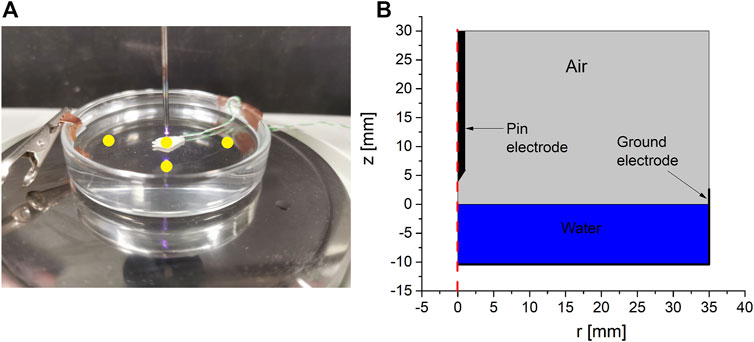
FIGURE 1. (A) A picture of the experimental setup used in this study and (B) the computational domain of the model representing the experimental setup. The yellow circles in panel a represent the points at which the temperature was measured. The point at the plasma contact point represents the thermocouple measurement at the bottom of the Petri dish.

For the three operating powers, the temperature of the treated water was recorded as a function of time at four points. Three points were on the surface of the water, while the fourth point was in the bulk of the water. The temperature of three out of the four points was measured using an infrared camera (FLIR E76 24°). The standoff distance of the camera was approximately 20 cm, which was enough to ensure that the resolution of the camera and the standoff distance had no influence on the measurements, as verified by having a reference temperature imaged at different standoff distances. The fourth point was measured using a type K thermocouple submerged in water and fixed at the center of the Petri dish. To prevent electric current from flowing into the thermocouple it was covered with a thermal paste, which served as an insulator for the current and as a conductor of heat, ensuring that the temperature recorded by the thermocouple was close to that of the bulk water. The four measurements were then averaged, and their standard deviation was computed. It was found that the standard deviation of the four measurements did not exceed 5% of the average temperature, indicating the consistency of the measurements.

3 Numerical model

The numerical model used in this study was the same as that reported in a previous work by the authors [24]. For brevity, a summary of the model description is given here while the upgrade of the model is discussed in detail. The model was defined in a two-dimensional axially symmetry domain describing a pin-to-water discharge configuration. It consisted of two components, an electric component and a mechanical component. The electric component described the plasma discharge between the pin and the surface of the water. It was a standard multifluid model that solved for the densities of N₂⁺, O₂⁺, and O₂⁻, electrons and electron energy density in addition to the electric potential in both phases. The choice of these specific species and the chemical kinetics associated with them was based on the findings of an earlier work of the authors [25], which identified the dominant charged species and their chemical pathways in a typical air plasma discharge. The electric component also solved for current conduction in the liquid phase. The electric component was solved for a single period of the waveform used in experiments. Considering that this type of discharge causes loading of the power supply, the applied voltage waveform used in the model was taken from experiments after averaging over multiple periods. The applied voltage waveform was semisinusoidal with a peak voltage of 3.5 kV and a frequency of 22 kHz. As the electric component was solved, the electrohydrodynamic (EHD) force field exerted by the plasma on the background gas was integrated in time to compute its time-averaged value to be used as input to the mechanical part. In its original version, the model also computed the electric field stresses at the interface; however, it was shown in previous work that the electric field stress at the interface dominates the behavior of the surface only for water with low conductivity [24]. Consequently, it was ignored in this work as the conductivity of the water samples was high enough for the electric field stresses at the surface to have negligible influence on the dynamics of the interface. After the electric component of the model was solved, the mechanical component was then solved. It described the flow dynamics in both phases by solving Navier–Stokes equations, in addition to solving for the deformation of the free surface using the arbitrary Lagrange–Eulerian (ALE) scheme. The mesh used in the model had a resolution of approximately 1 μm at the interface from both sides, while at the boundaries of the computational domain, the mesh resolution was in the order of 0.5 mm. Mesh convergence analysis has been conducted for the investigated work, and it was found that the solution is independent of the mesh used.

The upgrade to the model, equations describing heat and mass transfer across the interface were incorporated into the mechanical component of the model, as described in the following sections.

3.1 Addition of heat transfer in both phases

To solve for heat transfer in both phases, the heat equation, given by Eq. 1, was solved as part of the mechanical component.

$\mathit{\rho }{\mathit{C}}_{\mathit{p}}\left(\frac{\partial \mathit{T}}{\partial \mathit{t}}+\stackrel{\rightharpoonup }{\mathit{u}}\bullet \mathit{\nabla }\mathit{T}\right)=\mathit{\nabla }\bullet \left(-\mathit{\kappa }\mathit{\nabla }\mathit{T}\right)+\mathit{Q}.(1)$

In Eq. 1, ρ is the mass density of the fluid (kg˖m⁻³), which was calculated by the model in air as $\rho =P{M}_{avg}/\left(RT\right)$, where P is the pressure of the gas mixture (Pa), M_avg is the average molar mass of the mixture (kg mol⁻¹), R is the ideal gas constant, and T is the temperature (K). The density of water was defined as function of temperature [26] and C_p is the heat capacity at constant pressure (J K⁻¹), which was computed in air as $C_p=\sum {\omega }_i{C}_{pi}$, where ω_i is the mass fraction of the i^th constituent of the gas mixture and C_pi is the heat capacity of that constituent. In water, the value was defined as a function of temperature [26], and $\stackrel{\rightharpoonup }{u}$ is the velocity field computed by Navier–Stokes equations in the mechanical component (m s⁻¹). In the right-hand side of Eq. 1, κ is the heat conductivity (W m⁻¹k⁻¹) of both phases, set as a function of temperature in air [27] and to 0.61 in the liquid phase [28]. The last term, Q, is the volumetric heating term (W m⁻³). This term in the gas phase was set equal to the power lost through inelastic electron collisions with the background gas, which was computed in the electric component of the model. The inelastic collisions include rotational and vibrational excitation of the molecules of the background gas. In the liquid phase, the volumetric heating term was set equal to the ohmic heating due to current conduction by the solvated ions in the liquid. The concentration of the ions in the aqueous phase was adjusted such that the conductivity of the liquid matched that in experiments. The boundary condition at the external boundaries of the computational domain, as shown in Figure 1, imposed a zero-gradient condition on temperature for outflowing gas. For inflowing gas, the temperature is set equal to room temperature, mimicking an open boundary where the surrounding of the computational domain is held at room temperature.

At the interface, an energy balance condition was imposed as given in Eq. 2, where $\widehat{n}$ is the normal unit vector at the interface, pointing from the gas into the liquid. The square brackets on the left-hand side of Eq. 2 represent a jump condition, that is, the difference between the heat flux across the interface. The sum on the right-hand side runs over all plasma ionic species in the model, where E_i is the kinetic energy of the i^th species as it bombards the interface, Γ_I is the flux of the i^th species to the interface (m⁻² s⁻¹), R_(T) is the enthalpy of vaporization of water as a function of temperature (J kg⁻¹) [24], and J_H2O is the net flux of H₂O across the interface (kg m⁻²s⁻¹). Its calculation is explained in Section 3.2.

$\widehat{\mathit{n}}\bullet \left[\mathit{\kappa }\mathit{\nabla }\mathit{T}\right]={\displaystyle \sum }_{\mathit{i}}{\mathit{E}}_{\mathit{i}}{\mathit{\Gamma }}_{\mathit{i}}-{\mathit{R}}_{\left(\mathit{T}\right)}{\mathit{J}}_{{\mathit{H}}_{\mathbf{2}}\mathit{O}}.(2)$

The first term in the right-hand side of Eq. 2 describes heat flux from the plasma to the interface, which is computed by the electric component of the model. The flux is equal to the kinetic energy flux carried by the ionic species to the interface. It originates from the acceleration of the ions in the sheath. This treatment assumes that all of the kinetic energy of the ions is dissipated as heat in the liquid. Considering that other processes such as sputtering are possible, this treatment represents an upper limit to the heat flux due to the ions. The second term in the right-hand side of Eq. 2 represents the enthalpy of vaporization, which can be a loss term (i.e., causing the interface to cool) when the net flux of water is directed from the liquid phase into the gas phase, signifying vaporization or it can be a source term when the flux is reversed, representing the condensation of water vapor.

A single modification was performed to the Navier–Stokes equations, which involved adding a buoyancy force to the conservation of momentum equation. It was modeled as a volumetric force given in Eq. 3, where ρ₀ is the standard density of air at ambient conditions (kg m⁻³), set equal to 1.24, and g is the gravity acceleration in the z direction, set equal to 9.81 (m s⁻²).

${\stackrel{\rightharpoonup }{\mathit{F}}}_{\mathit{b}\mathit{o}\mathit{u}\mathit{y}\mathit{a}\mathit{n}\mathit{c}\mathit{y}}=\left({\mathit{\rho }}_{\mathbf{0}}-\mathit{\rho }\right)\stackrel{\rightharpoonup }{\mathit{g}.}(3)$

3.2 Addition of mass transfer in the gas phase

Since an increase in the temperature of water increases its vapor pressure, it is important to follow that increase and its spatial variation as it affects the chemistry of the gas phase. As any increases in temperature of the liquid was followed by the mechanical component of the model, following the water vapor content in the gas phase should follow on the same timescale. Thus, two additional equations were added to the mechanical component to solve for the mass fraction of O₂ and H₂O, as given in Eq. 4. The mass fraction of the remaining constituent, N₂, was determined from the constraint that the sum of all mass fractions is equal to 1.

$\mathit{\rho }\frac{\partial {\mathit{\omega }}_{\mathit{k}}}{\partial \mathit{t}}+\mathit{\nabla }\bullet \left(-\mathit{\rho }{\mathit{D}}_{\mathit{k}}\mathit{\nabla }{\mathit{\omega }}_{\mathit{k}}-\mathit{\rho }{\mathit{\omega }}_{\mathit{k}}{\mathit{D}}_{\mathit{k}}\mathit{\nabla }{\mathit{M}}_{\mathit{n}}-\frac{\mathit{\rho }{\mathit{\omega }}_{\mathit{k}}}{{\mathit{M}}_{\mathit{n}}}{\displaystyle \sum }_{\mathit{l}}{\mathit{M}}_{\mathit{l}}{\mathit{D}}_{\mathit{l}}\mathit{\nabla }{\mathit{x}}_{\mathit{l}}\right)+\mathit{\rho }(\stackrel{\rightharpoonup }{\mathit{u}}\bullet \mathit{\nabla }){\mathit{\omega }}_{\mathit{k}}=\mathbf{0}.(4)$

Most of the parameters in Eq. 4 were defined earlier; x_k is the mole fraction of the k^th species, and D_k is the diffusion coefficients of the k^th species in the mixture (m²s⁻¹), which were determined from binary diffusion coefficients using Eq. 5, where D_ik is the binary diffusion coefficient of the i^th species into the k^th species, which was determined using the mixture-averaged formulation [29].

${\mathit{D}}_{\mathit{k}}=\frac{\mathbf{1}-{\mathit{\omega }}_{\mathit{k}}}{{{\displaystyle \sum }}_{\mathit{i}\ne \mathit{k}}\frac{{\mathit{x}}_{\mathit{i}}}{{\mathit{D}}_{\mathit{i}\mathit{k}}}}.(5)$

The plasma–liquid interface is treated as a flux source described by a balance between vaporization flux and condensation flux. Multiple expressions to describe this balance are available in the literature, the most common of which is given by the Hertz–Knudsen formulation [30]. Despite its wide use, this formulation does not satisfy the conservation of momentum and energy at the interface nor is it applicable to situations where nonsoluble gases exert pressure on the liquid [29, 31], as is the case in the current investigation. An alternative formulation, the Schrage formulation, overcomes both limitations [29]; therefore, it was used in this work, as given in Eq. 6.

${\mathit{J}}_{{\mathit{H}}_{\mathbf{2}}\mathit{O}}=\mathit{\alpha }\sqrt{\frac{\mathit{R}}{\mathbf{2}\mathit{\pi }{\mathit{M}}_{{\mathit{H}}_{\mathbf{2}}\mathit{O}}}}\left({\mathit{\rho }}_{\mathit{s}\mathit{a}\mathit{t}\left({\mathit{T}}_{\mathit{L}}\right)}\sqrt{{\mathit{T}}_{\mathit{L}}}-{\mathit{\Gamma }}_{\left({\mathit{v}}_{\mathit{R}}\right)}{\mathit{\rho }}_{\mathit{v}}\sqrt{{\mathit{T}}_{\mathit{G}}}\right).(6)$

In Eq. 6, α is the fraction of gaseous water molecules that strike the interface and accommodate to the liquid phase. Molecular dynamics simulations showed that a typical value of this variable is close to 1 at the boiling temperature of water [29], therefore it was set to 1 in this expression, M_H2O is the molecular weight of water (kg mol⁻¹), ρ_sat is the saturation vapor density at a given temperature of the liquid (kg m⁻³), and T_L and T_G are the temperatures of the interface from the liquid and the gas side, respectively. The two temperatures are not necessarily equal, and a temperature jump is reported for certain conditions [30, 32]. However, it was shown that as the pressure approaches atmospheric pressure, the jump in the temperature gradually disappears and the temperature in the liquid side of the interface is equal to that in the gas side [31]; hence, in this work it was assumed that T_G = T_L, ρ_v is the vapor pressure on the gas side of the interface (kg m⁻³), and lastly Γ(v_R) is a kinetic function of the velocity of the macroscopic water vapor velocity, which describes the flux to the interface from the gas phase, as given in Eq. 7. In this equation, v_R is the ratio of the macroscopic velocity of water molecules to the thermal velocity of water vapor at a given temperature and erf is the error function. The macroscopic velocity was set equal to the gas velocity at the interface.

${\mathit{\Gamma }}_{\left({\mathit{v}}_{\mathit{R}}\right)}={\mathit{e}}^{-{\mathit{v}}_{\mathit{R}}^{\mathbf{2}}}-{\mathit{v}}_{\mathit{R}}\mathit{\pi }\left[\mathbf{1}-\mathit{erf}\left({\mathit{v}}_{\mathit{R}}\right)\right].(7)$

3.3 Iteration between mechanical and electric components

Initially, the experimental parameters were input to the electric component. These include the geometry, the volume of water, and the distance between the tip of the pin electrode and the surface of the water, in addition to the voltage waveforms recorded in experiments. The electric part was then solved for one period, after which time-average quantities were extracted and input into the mechanical part. The output from the electric part to the mechanical part included the EHD forces in the gas phase, the heat flux of the ions in the plasma to the interface, the discharge power lost to the background gas as heat through inelastic collisions driven by electrons, and the ohmic heating of the liquid due to current conduction by aqueous ions. The mechanical component is then solved for 100 s. After which, the shape of the interface, the flow velocities in both phases, and the gas pressure are fed back into the electric component. This represents a single iteration of the model. The results presented in Section 4 were obtained after two iterations, unless otherwise stated.

4 Results and discussion

The model was solved for three cases similar to those investigated in experiments. The power computed by the model was evaluated as the integration of the current density on the surface of the pin electrode multiplied by the applied voltage, thus giving the computed operating power, which was found to deviate by less than 15% from the corresponding experimental power for any given case.

4.1 Experimental validation

To validate the model, the computed temperature in the liquid phase was averaged over the liquid volume and compared to the average liquid temperature measured experimentally as a function of time. Figure 2 shows that there is a reasonable agreement between the model and experiments, where the model follows the trends observed experimentally, both qualitatively and quantitively. Focusing on differences, the model slightly overestimates the liquid temperature. This was attributed to the assumption that all of the kinetic energy of the bombarding ions is dissipated as heat, ignoring processes such as sputtering, which has been shown to take place at plasma–liquid interfaces for ions with an energy greater than 10 eV [33, 34]. Another possible cause of this difference is ignoring the thermal boundaries of the system, where the model assumed the system was thermally isolated from its environment while the experimental setup was placed on a metallic surface.

FIGURE 2

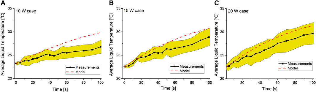
FIGURE 2. Comparison between the computed and measured average liquid temperature as a function of time for operating powers (A) 10 W, (B) 15 W, and (C) 20 W. The solid black line shows the measured average temperature of the liquid, the dashed red line shows the computed average temperature, and the yellow shaded region shows the standard deviation of the experimental measurements.

Another difference is the sensitivity of the average liquid temperature to the variation in the operating power, which was underestimated by the model in comparison to experiments. This was attributed to keeping the conductivity of the liquid media constant in the model. It has been shown in multiple experimental works that treating a liquid medium with plasma increases its conductivity noticeably even on a short timescale [8, 35]. Assuming the operating power is constant, an increase in the liquid’s conductivity means that the power dissipated in the liquid is reduced, thus leaving a larger fraction of the operating power to be dissipated in the plasma and therefore enhancing all of the heating mechanisms driven by the plasma. Since the model does not capture the variation of the conductivity of the liquid due to plasma treatment, the variation in the computed discharge power is less than that in experiments.

4.2 Liquid temperature

The two-dimensional distribution of temperature in the liquid for the three investigated cases is shown in Figure 3 at the end time of the simulation, that is, 100 s after plasma ignition.

FIGURE 3

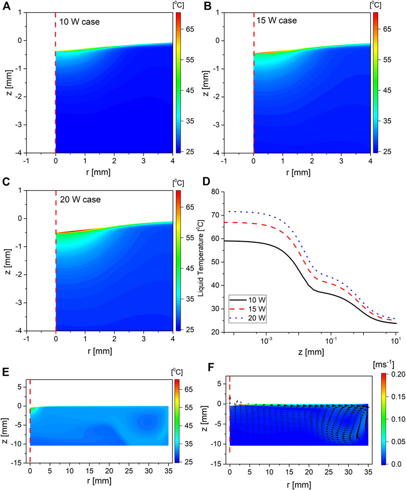
FIGURE 3. Two-dimensional color map of the temperature in the liquid phase for the operating powers (A) 10 W, (B) 15 W, and (C) 20 W. Panels (A–C) have the same color legend. Panel (D) shows the liquid temperature plotted along the symmetry axis for the three cases, where z = 0 is at the interface; panel (E) shows the temperature in the entire liquid part of the computational domain for the 15 W case, and panel (F) shows the magnitude of the flow velocity in the liquid phase as background color, with the direction indicated by the imposed arrows. All of the data shown in this figure were taken at t = 100 s, where t = 0 is the time at which the plasma was ignited.

The liquid temperature had a similar distribution irrespective of the operating power. The liquid temperature can be split into three zones. Moving from the interface toward the bulk, the first zone is a thin film of hot liquid that exists at the interface with a typical depth of 10 μm, followed by the second zone, which is a region of relatively cooler liquid extending up to 1 mm from the interface, and finally, the third zone represents the bulk region, where the temperature is almost uniform. The impact of increasing the operating power is mostly manifested as a scaling of the temperature profile rather than changing its spatial distribution. To investigate the origin of these zones, the mechanical component of the model was run with the heating mechanism selectively switched in order to quantify their contributions to each zone. The thin film zone forms as a result of the ionic heating flux and the thermal boundary layer due to the flow of hot gas in the plasma side of the interface. Moreover, it has been reported from molecular dynamics studies that impinging ions on a water sample dissipate their energy in the first few monolayers, extending to a few nanometers in depth from the interface [32]. Since the ionic heat flux is dominated by the plasma side of the interface, the temperature at the interface increases until the temperature gradient is steep enough for the conductive heat transfer on the liquid side to establish local thermal equilibrium at the interface. Since conductive heat transfer is diffusive by nature, the width of the thin layer zone is larger than the thickness of the few monolayers where ions dissipate most of their kinetic energy. Furthermore, contrasting the characteristics of the thin film reported here with a typical thermal boundary layer encountered at a hot gas–liquid interface, the width of the thin layer zone was found to be consistent with that of a thermal boundary layer in the liquid phase, which was estimated by running the heat transfer part of the model with a hot gas blowing at the interface in the absence of plasma. The ionic heat flux only increased the temperature, thus causing a steeper temperature gradient at the interface. Moving to the second zone, where the temperature drops to approximately 66% of that at the interface, the temperature in this region is above that in the bulk liquid by approximately 15°C. This above-bulk temperature is maintained by the ionic ohmic heating in the liquid, which is concentrated in this region due to the small surface area at the interface through which the current flows; thus, the local current density at that point is the highest in the liquid volume, resulting in the maximum volumetric heating in the liquid phase. Lastly, moving to the bulk of the liquid which is at a significantly lower temperature than the interface, it is heated by convection from the interface, which can be seen clearly in Figure 3E as the distribution of the hot liquid matches the convection pattern encountered in this type of discharge [24, 36], shown in Figure 3F for this investigated case.

While the chemistry of the discharge is beyond the scope of this work, the implications of the findings presented here are quite significant for the transport of the gaseous species across the interface. As the temperature of the liquid is increased, Henry coefficients, which describe the solubility of gaseous species in the liquid, decrease. For the highest reported temperature increase in this work, for the 20 W case, the value of Henry’s coefficient of O₃ decreases to 35% of its value at ambient conditions. Similar figures for H₂O₂ and OH are 4.8% and 9%, respectively [14]. Accordingly, the presence of the thin film at the interface represents a solvation barrier for the species generated in the gas phase, hinting that the role of aqueous reactions in generating aqueous species is more significant than previously thought.

4.3 Gas temperature and gas rarefaction

Considering that the heat capacity of the gas is much smaller than that of water, its temperature was computed using two different approaches, the standard approach where all heating terms were averaged over the duration of the period, then solved as part of the mechanical components as explained in Section 3. The second approach was to solve the mechanical component using instantaneous heating terms as the electric component of the model was solved. This allowed for a comparison of the temperature observed on different timescales. The two-dimensional distribution of gas temperature for both approaches is shown in Figure 4, where panel 1) shows the temperature computed using the time-averaged heating terms for the 15 W case, while panel 2) shows the temperature computed using the instantaneous heating terms for the same case.

FIGURE 4

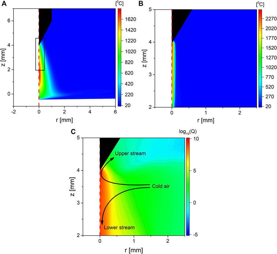
FIGURE 4. Two-dimensional color map showing (A) the gas temperature computed using the time-averaged heating term for operating power of 15 W, (B) the gas temperature computed using instantaneous heating terms for operating power of 15 W, the domain shown in panel b is indicated as a black box, and in panel (A,C), the logarithm of the time-average heating term of the background by the plasma for the 15 W case.

From Figure 4, it can be seen that the maximum temperature is consistent with that reported in the literature for similar discharge types [13, 20, 22, 23]. An interesting difference between panels a and b in Figure 4 is that the maximum gas temperature, equal to 1,745 and 2,563°C in panels a and b, respectively, is located at the middle of the discharge gap instead of the tip of the electrode as shown in panel a, which is in contrast to that shown in panel b and what is typically expected in such type of discharges20 22. This difference is likely the result of two processes: heat coupling to the gas flow and gas rarefaction. As shown in the previous work of the authors [24] and as highlighted in Figure 4C, the gas flow induced by the EHD force pushes the air out of the discharge in two streams. The first stream (upper stream) leaves the discharge gap close to the pin electrode, where the flow is directed upward due to EHD forces exerted in the sheath at the tip of the electrode. The second stream (lower stream) originates in the bulk plasma channel, where the EHD forces push the air downward toward the surface of the liquid, causing the air to leave the discharge gap at the interface as radially expanding flow. As a result of air being pushed out from the discharge gap, cold air flows from the side of the discharge gap. The fate of the cold air depends on the stream it becomes part of. The upper stream passes close to the pin tip, which is the position of the maximum heating power as Figure 4C shows. However, because it has a short residence time, it gets pushed out from that region by the background flow before it is heated significantly. On the other hand, the lower stream travels through the plasma channel until it arrives at the interface. This yields a significant residence time, such that the moving air experiences multiple streamers as it is traveling downward and therefore experiences more heating than the stream traveling upward, as indicated in Figure 4C. Considering that the timescale of the development of the flow is typically in the millisecond range [37], which is much longer than a single period of the waveform, the coupling between the background flow and gas heating can be observed only using the time-averaged heating terms approach. This process has important implications for temperature-sensitive species such as O₃, as it implies such species are most likely to exit the discharge region through the upper stream, making the delivery of such species to the interface less efficient, assuming the discharge conditions allow for such species to form.

The second process is gas rarefaction, where the ideal gas law predicts that at the temperatures shown in Figure 4, the gas density will drop to 16% of its value at ambient conditions. However, such a simple calculation cannot predict the consequences on the discharge behavior. To quantify this, the solution from the first iteration (i.e., without accounting for rarefaction) was compared to the solution from the second iteration (accounting for rarefaction). The comparison was focused on the spatial distribution of the plasma heating power of the background gas in addition to the ionic heat flux at the interface.

Figure 5 shows that the rarefied density is consistent with the ideal gas law. Furthermore, Figure 5B shows the plasma power dissipated as heat (which can be referred to as heating power) to the background gas with and without gas rarefaction. It is clear that when gas rarefaction was accounted for the heating power close to the tip of the electrode decreased, while the heating power in the discharge gap increased by more than an order of magnitude. This explains the shift in the maximum temperature observed in Figure 4. Another implication of the gas rarefaction is emphasized in Figure 5C, which shows the time-averaged ionic heating flux at the interface. The time-averaged heat flux was computed as the integral of the product of the ion flux arriving at the interface multiplied by its average kinetic energy (the first term in the right-hand side of Eq. 2), which is then integrated over the period and divided by it. When gas rarefaction was accounted for, the ionic heat flux to the interface was increased by a factor of 3, which is a result of the increased mean free path in the sheath. It should be noted here that the comparison shown in Figure 5 was conducted using similar operating powers. The trends reported here were consistent among all investigated operating powers.

FIGURE 5

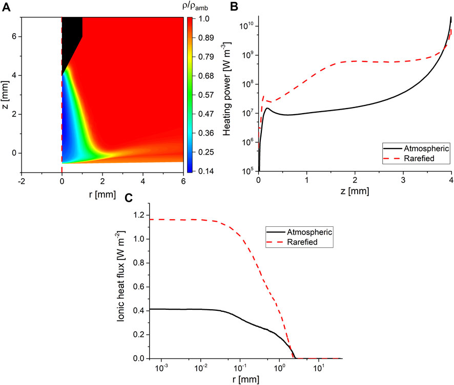
FIGURE 5. (A) Two-dimensional color map showing the density of the background gas normalized to its value at ambient conditions, (B) plasma power dissipated as heat to the background gas along the symmetry axis with and without gas rarefaction considered, z = 4 is the tip of the pin electrode and z = 0 is the interface, and (C) the time-averaged ionic heat fluxes to the interface with and without gas rarefaction. The data shown in all panels of the figure are for an operating power of 15 W.

Figures 4, 5 also show that close to the interface, there is a pocket of gas where the impact of the plasma heating is smaller than that observed in the discharge gap. This is a result of the high water vapor content in that pocket, as will be explained in Subsection 4.4.

4.4 Water vapor density in the gas phase

Considering that the plasma causes the formation of a thin film of hot liquid at the interface, as explained in Section 4.2, while simultaneously causing gas rarefaction, as explained in Section 4.3, both effects contribute toward promoting water vaporization. Figure 6 shows a zoomed-in view at the interface and depicts the percentage of water vapor in the overall gas mixture for the 15 W case.

FIGURE 6

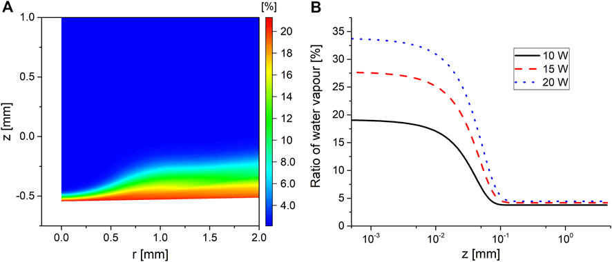
FIGURE 6. (A) Percentage of water vapor in the gas mixture for operating power of 15 W at t = 100 s and (B) the percentage of the water vapor in the gas mixture along the symmetry axis for the three investigated operating powers, where z = 0 is the interface.

Figure 6 shows that the water vapor makes up to 25% of the total gas composition in a region that extends up to 0.1 mm above the interface in the plasma phase. The height of this layer is at its minimum on the symmetry axis as a result of the stagnation pressure due to the impinging flow at the interface from the plasma phase. Moving radially outward, the flow expands in width while at the same time carrying the water vapor vaporized close to the symmetry axis, resulting in a widening of the water vapor layer at the interface. The relatively high content of water vapor was enough to cause the mixture’s heat capacity to increase by 25% in the water vapor layer, explaining the pocket of dense gas observed in Figure 5A at the interface.

The model was only solved for 100 s, which was not enough to reach the boiling temperature of water under the investigated conditions. The model was run while artificially increasing the heat flux to the interface in order to determine the corresponding water vapor percentage at boiling conditions. It was found that the maximum water vapor content ranged between 70% and 80% of the total gas composition at the interface, with the specific ratio being dependent on the convection from the gas phase.

The implications of the width of the vapor layer and its gas composition can be appreciated when comparing its width to the width of the plasma sheath, which was found to be of the order of 50 μm under the investigated conditions. This means that a significant proportion of the collisions encountered by the ions as they travel from the plasma to the liquid are with water molecules. Considering that the mean free path of a molecule at ambient conditions in water vapor can be 30 times larger than that in dry air [32], it is expected that the water vapor layer reported here will significantly impact the ion energy distribution function at the interface. Furthermore, during the negative cycle of the discharge, the sheath at the plasma–liquid interface will be dominated by electrons. Having a higher water vapor concentration than ambient air implies that the chemistry driven by the electrons will experience a transition from being dominated by long-lived species typically encountered in air plasmas such as O₃ and NO₂ to being dominated by water-based species such as OH. The water vapor concentration at which such a transition occurs remains to be investigated.

5 Conclusion

In this work, a 2D numerical model describing a pin–water discharge configuration and operating in air under ambient conditions was upgraded to account for heat and mass transfer processes in both phases. The model was validated in terms of the predicted average water temperature and was found to have reasonable agreement with experimental measurements.

The model was used to analyze the spatial distribution of the liquid temperature, where it was reported that the liquid can be split into three zones: the first zone is the interface zone, where a thin film of liquid at a temperature three times higher than the bulk temperature extends up to 10 μm in depth, followed by a cooler region with a temperature equal to 66% of that at the interface, extending up to 1 mm from the interface, and then followed by the bulk of the liquid, which is at a much lower temperature than the interface, with an almost uniform temperature distribution.

On the gas side of the interface, it was found that the plasma heats the background gas to approximately 1,700–2,600°C for the investigated conditions in this work, causing the density of the background gas to drop to 15% of its value at ambient conditions. This gas rarefaction combined with the induced flow by EHD forces caused the maximum temperature in the discharge region to shift from the tip of the electrode to the center of the discharge gap on long timescales.

The combined effect of gas rarefaction and liquid heating promoted the vaporization of water, where the gas composition on the plasma side of the interface was analyzed. It was observed that a thin layer of water vapor extends to 0.1 mm above the interface, where the water vapor constitutes between 20% and 35% of the total gas composition for the conditions investigated in this work. Extrapolating these conditions to the boiling point of water increased the water vapor fraction to 70%–80%.

The findings of this work have many implications on the current understanding of plasma–liquid interaction. First, the presence of a thin film of hot liquid at the interface represents a solvation barrier for gaseous species, thus reducing their anticipated role in aqueous chemistry. Second, the coupling between heat transfer and gas flow indicates that temperature-sensitive species such as O₃ might be extracted from the discharge region toward the pin electrode rather than toward the interface, as that stream has a lower temperature on average and thus a longer life time of O₃. Third, this work reported that the thickness of the thin water vapor layer on the plasma side of the interface is larger than the plasma sheath, implying the dominance of water-based species at the interface in addition to a significant alternation of the ion energy distribution function as ions arrive at the interface.

Data availability statement

The raw data supporting the conclusion of this article will be made available by the authors, without undue reservation.

Author contributions

The work was conceptualized by JS and MH who performed the modeling part. The experimental part was performed by AD and JW. All authors have approved the manuscript.

Funding

This work was supported by EPSRC grant numbers EP/S025790/1, EP/N021347/1, and EP/T000104/1.

Acknowledgments

JW and MH acknowledge the financial support of EPSRC. For the purpose of Open Access, the author has applied a Creative Commons Attribution (CC-BY) license to any Author Accepted Manuscript version arising.

Conflict of interest

The authors declare that the research was conducted in the absence of any commercial or financial relationships that could be construed as a potential conflict of interest.

Publisher’s note

All claims expressed in this article are solely those of the authors and do not necessarily represent those of their affiliated organizations, or those of the publisher, the editors, and the reviewers. Any product that may be evaluated in this article, or claim that may be made by its manufacturer, is not guaranteed or endorsed by the publisher.

References

1. Nastuta AV, Topala I, Grigoras C, Pohoata V, Popa G. Stimulation of wound healing by helium atmospheric pressure plasma treatment. J Phys D: Appl Phys (2011) 44, 105204. doi:10.1088/0022-3727/44/10/105204

CrossRef Full Text | Google Scholar

2. Ranieri P, Sponsel N, Kizer J, Rojas-Pierce M, Hernández R, Gatiboni L. Plasma agriculture: Review from the perspective of the plant and its ecosystem. Plasma Process Polym (2021) 18–2000162. doi:10.1002/ppap.202000162

CrossRef Full Text | Google Scholar

3. Attri P, Yusupov M, Park JH, Lingamdinne LP, Koduru JR, Shiratani M, et al. Mechanism and comparison of needle-type non-thermal direct and indirect atmospheric pressure plasma jets on the degradation of dyes. Sci Rep (2016) 6–34419. doi:10.1038/srep34419

PubMed Abstract | CrossRef Full Text | Google Scholar

4. Jović MS, Dojcinovic BP, Kovacevic VV, Obradovic BM, Kuraica MM, Gasic UM, et al. Effect of different catalysts on mesotrione degradation in water falling film DBD reactor. Chem Eng J (2014) 248:63–70. doi:10.1016/j.cej.2014.03.031

CrossRef Full Text | Google Scholar

5. Toth JR, Abuyazid NH, Lacks DJ, Renner JN, Sankaran RM. A plasma-water droplet reactor for process-intensified, continuous nitrogen fixation at atmospheric pressure. ACS Sustain Chem Eng (2020) 8:39 14845–54. doi:10.1021/acssuschemeng.0c04432

CrossRef Full Text | Google Scholar

6. Zeghioud H, Nguyen-Tri P, Khezami L, Amrane A, Assadi AA. Review on discharge plasma for water treatment: Mechanism, reactor geometries, active species and combined processes. J Water Process Eng (2020) 38–101664. doi:10.1016/j.jwpe.2020.101664

CrossRef Full Text | Google Scholar

7. Hoeben WFLM, van Ooij PP, Schram DC, Huiskamp T, Pemen AJM, Lukes P. On the possibilities of straightforward characterization of plasma activated water. Plasma Chem Plasma Process (2019) 39:597–626. doi:10.1007/s11090-019-09976-7

CrossRef Full Text | Google Scholar

8. Judée F, Simon S, Bailly C, Dufour T. Plasma-activation of tap water using DBD for agronomy applications: Identification and quantification of long lifetime chemical species and production/consumption mechanisms. Water Res (2018) 133:47–59. doi:10.1016/j.watres.2017.12.035

PubMed Abstract | CrossRef Full Text | Google Scholar

9. Shaer ME, Eldaly M, Heikal G, Sharaf Y, Diab H, Mobasher M., et al. Chem Plasma Process Plasma(2020) 40:971. doi:10.1007/s11090-020-10076-0

CrossRef Full Text | Google Scholar

10. Medvecká V, Mosovska S, Mikulajova A, Valik L, Zahoranova A. Cold atmospheric pressure plasma decontamination of allspice berries and effect on qualitative characteristics. Eur Food Res Technol (2020) 246:2215–23. doi:10.1007/s00217-020-03566-0

CrossRef Full Text | Google Scholar

11. Lindsey A, Anderson C, Slikboer E, Shannon S, Graves D. Cold atmospheric pressure Journal J Phys D: Appl Phys (2015) 48–424007. doi:10.1088/0022-3727/48/42/424007

CrossRef Full Text | Google Scholar

12. Hamdan A, Ridani DA, Diamond J, Daghrir R. Pulsed nanosecond air discharge in contact with water: Influence of voltage polarity, amplitude, pulse width, and gap distance. J Phys D Appl Phys (2020) 53–355202. doi:10.1088/1361-6463/ab8fde

CrossRef Full Text | Google Scholar

13. Bruggeman P, Liu J, Degroote J, Kong MG, Vierendeels J, Leys C, et al. Dc excited glow discharges in atmospheric pressure air in pin-to-water electrode systems. J Phys D Appl Phys (2008) 41–215201. doi:10.1088/0022-3727/41/21/215201

CrossRef Full Text | Google Scholar

14. Ono R Rapid temperature increase near the anode and cathode in the afterglow of a pulsed positive streamer discharge. J Phys D Appl Phys (2018) 51:245202. doi:10.1088/1361-6463/aac31d

CrossRef Full Text | Google Scholar

15. Takeuchi N, Ishii Y, Yasuoka K. Modelling chemical reactions in dc plasma inside oxygen bubbles in water. Plasma Sourc Sci Technol (2012) 21–015006. doi:10.1088/0963-0252/21/1/015006

CrossRef Full Text | Google Scholar

16. Pang B, Liu Z, Zhang H, Wang S, Gao Y, Xu D, et al. Investigation of the chemical characteristics and anticancer effect of plasma-activated water: The effect of liquid temperature. Plasma Process Polym (2022) 19:2100079. doi:10.1002/ppap.202100079

CrossRef Full Text | Google Scholar

17. Zhang X, Lee BJ, Im HG, Cha MS. Ozone production with dielectric barrier discharge: Effects of power source and humidity. IEEE Trans Plasma Sci (2016) 44:2288–96. doi:10.1109/TPS.2016.2601246

CrossRef Full Text | Google Scholar

18. Moiseev T, Misra NN, Patil S, Cullen PJ, Bourke P, Keener KM, et al. Post-discharge gas composition of a large-gap DBD in humid air by UV–Vis absorption spectroscopy. Plasma Sourc Sci Technol (2014) 23–065033. doi:10.1088/0963-0252/23/6/065033

CrossRef Full Text | Google Scholar

19. Abdelaziz AA, Ishijima T, Osawa N, Seto T. Quantitative analysis of ozone and nitrogen oxides produced by a low power miniaturized surface dielectric barrier discharge: Effect of oxygen content and humidity level. Plasma Chem Plasma Process (2019) 39:165–85. doi:10.1007/s11090-018-9942-y

CrossRef Full Text | Google Scholar

20. Komuro A, Ono R Two-dimensional simulation of fast gas heating in an atmospheric pressure streamer discharge and humidity effects. J Phys D Appl Phys (2014) 47–155202. doi:10.1088/0022-3727/47/15/155202

CrossRef Full Text | Google Scholar

21. Xu SF, Zhong XX, Majeed A. Neutral gas temperature maps of the pin-to-plate argon micro discharge into the ambient air. Phys Plasmas (2015) 22–033502. doi:10.1063/1.4913654

CrossRef Full Text | Google Scholar

22. Kacem S, Ducasse O, Eichwald O, Yousfi M, Meziane M, Sarrette JP, et al. Simulation of expansion of thermal shock and pressure waves inducaed by a streamer dynamics in positive DC corona discharges. IEEE Trans Plasma Sci (2013) 41:942–7. doi:10.1109/TPS.2013.2249118

CrossRef Full Text | Google Scholar

23. Agnihotri A, Hundsdorfer W, Ebert U. Modeling heat dominated electric breakdown in air, with adaptivity to electron or ion time scales. Plasma Sourc Sci Technol (2017) 26–095003. doi:10.1088/1361-6595/aa8571

CrossRef Full Text | Google Scholar

24. Dickenson A, Walsh JL, Hasan MI. Electromechanical coupling mechanisms at a plasma–liquid interface. J Appl Phys (2021) 129–213301. doi:10.1063/5.0045088

CrossRef Full Text | Google Scholar

25. Hasan MI, Walsh JL. Numerical investigation of the spatiotemporal distribution of chemical species in an atmospheric surface barrier-discharge. J Appl Phys (2016) 119–203302. doi:10.1063/1.4952574

CrossRef Full Text | Google Scholar

26. Crc Handbook of Chemistry and Physics . CRC handbook of chemistry and Physics. 95th ed., 6 (2015).section

27. Nist Chemistry WebBook. Beijing (2022).accessed in March

28. Becker M. Heat transfer: A modern approach. New York: Plenum Press (1986). chapter 1.

Google Scholar

29.“Chemically reacting flow” 2018, 2nd ed., John Wiley & Sons, chapter 2, Beijing China

30. Bird E, Gutierrez Plascencia J, Keblinski P, Liang Z. Molecular simulation of steady-state evaporation and condensation of water in air. Int J Heat Mass Transf (2022) 184–122285. doi:10.1016/j.ijheatmasstransfer.2021.122285

CrossRef Full Text | Google Scholar

31. Jafari P, Masoudi A, Irajizad P, Nazari M, Kashyap V, Eslami B, et al. Evaporation mass flux: A predictive model and experiments. Langmuir (2018) 34:11676–84. doi:10.1021/acs.langmuir.8b02289

PubMed Abstract | CrossRef Full Text | Google Scholar

32. Gatapova EY, Graur IA, Kabov OA, Aniskin VM, Filipenko MA, Sharipov F, et al. The temperature jump at water – air interface during evaporation. Int J Heat Mass Transf (2017) 104:800–12. doi:10.1016/j.ijheatmasstransfer.2016.08.111

CrossRef Full Text | Google Scholar

33. Minagawa Y, Shirai N, Uchida S, Tochikubo F. Analysis of effect of ion irradiation to liquid surface on water molecule kinetics by classical molecular dynamics simulation. Jpn J Appl Phys (2008) (2014) 53–010210. doi:10.7567/JJAP.53.010210

CrossRef Full Text | Google Scholar

34. Nikiforov AY. Plasma sputtering of water molecules from the liquid phase by low-energy ions: Molecular dynamics simulation. High Energ Chem (2008) 42:235–9. doi:10.1134/S0018143908030090

CrossRef Full Text | Google Scholar

35. Olszewski P, Li J, Liu D, Walsh J. Optimizing the electrical excitation of an atmospheric pressure plasma advanced oxidation process. J Hazard Mater (2014) 279:60–6. doi:10.1016/j.jhazmat.2014.06.059

PubMed Abstract | CrossRef Full Text | Google Scholar

36. Semenov IL, Weltmann KD, Loffhagen D. Modelling of the transport phenomena for an atmospheric-pressure plasma jet in contact with liquid. J Phys D Appl Phys (2019) 52–315203. doi:10.1088/1361-6463/ab208e

CrossRef Full Text | Google Scholar

37. Dickenson A, Britun N, Nikiforov A, Leys C, Hasan MI, Walsh JL. The generation and transport of reactive nitrogen species from a low temperature atmospheric pressure air plasma source. Phys Chem Chem Phys (2018) 20:28499–510. doi:10.1039/C8CP05762A

PubMed Abstract | CrossRef Full Text | Google Scholar