 Michael S. Murillo
- Department of Computational Mathematics, Science and Engineering, Michigan State University, East Lansing, MI, United States
A wide range of theoretical and computational models have been developed to predict the electrical transport properties of dense plasmas, in part because dense plasma experiments explore order-of-magnitude excursions in temperature and density; in experiments with mixing, there may also be excursions in stoichiometry. In contrast, because high pressures create transient and heterogeneous plasmas, data from experiments that isolate transport are relatively rare. However, the aggregate of our datasets continues to increase in size and plays a key role in the validation of transport models. This trend suggests the possibility of using the data directly to make predictions, either alone or in combination with models, thereby creating a predictive capability with a controllable level of agreement with the data. Here, such a data-driven model is constructed by combining a theoretical model with extant data, using electrical conductivity as an example. Discrepancy learning is employed with a theoretical model appropriate for dense plasmas over wide ranges of conditions and a dataset of electrical conductivities in the solid to expanded warm dense matter regimes. The resulting discrepancy is learned via a radial basis function neural network. Regularization of the network is included through centers chosen with silhouette scores from k-means clustering. The covariance properties of each cluster are used with a scaled Mahalanobis distance metric to construct anisotropic basis functions for the network. The scale is used as a hyperparameter that is used to optimize prediction quality. The resulting predictions agree with the data and smoothly transition to the theoretical model away from the data. Detailed appendices describe the electrical conductivity model and compare various machine-learning methods. The electrical conductivity data and a library that yields the model are available at GitHub.
1 Introduction
Dense plasmas are typically created in the laboratory by heating solids with currents, radiation or beams. In all cases, electron-ion collisions play a central role in determining the characteristics of the energy absorption. Energy deposition properties (e.g., stopping range) from ion beams, for example, are primarily determined by projectile-electron collisions [1]. Similarly, properties of laser absorption are also determined by electron-ion collisions in the inverse Bremsstrahlung process [2, 3]. These energy-deposition processes are typically characterized by the stopping-power and electrical-conductivity transport coefficients. Knowledge of these coefficients allows us to design and interpret experiments and provides physical insight into material properties. In fact, these transport coefficients, together with the equation of state [4], are the closures in hydrodynamics models that specify material properties [5–7]. It is important to obtain accurate values for these coefficients, but it is difficult to do so over large ranges of material properties because of the order-of-magnitude excursions in these properties during a typical experiment. This difficulty poses challenges for theoretical and computational approaches that are highly efficient in narrow regimes of material properties.
A typical research pattern is that theoretical and/or computational models are compared to each other, yielding a form of theoretical confidence or sensitivity [4, 7], and are validated with experimental data. With increasing amounts of experimental data becoming available, an alternate approach, using machine learning (ML), is possible: rather than merely validating models with data, data can now be directly employed in generating models. ML approaches to capturing and predicting material properties are currently under intense development [8–11], and such approaches are widely used in plasmas physics [12]. Other applications of ML in plasma physics include, for example, mitigating disruptions that break confinement in tokamaks, provided accurate forecasts can be made from real-time data; in fact, using a wide variety of ML techniques, the success rate for predicting disruptions is quite high [13]. Another example is the use of ML to produce clean gases from biomass by predicting chemical processes in plasma arcs to improve tar removal [14]; in general, ML has numerous uses in low-temperature plasma applications [15, 16]. Closer to the theme of this work, artificial neural networks have been used to reconstruct plasma parameters using spectra from laser-plasma experiments [17]. Here, ML will be used to develop predictions for the electrical conductivity in dense plasmas, both as an exemplar of this approach and because of the intrinsic importance of the electrical conductivity in plasma applications.
A wide array of theoretical and computational methods has been developed across many decades to model electrical conductivities [18–21]. The ongoing need for new models stems from the fact that practical models are formulated for a narrow range of material properties; theoretical and computational approaches are efficient and accurate in limited regimes [7]. This can be seen by considering the Lee-More model of electronic transport [18], a version of which is developed in this work. To account for large changes in material properties, the Lee-More model uses a “patchwork-quilt” approach that stitches together conductivity models appropriate in different regimes of temperature-density space (see their Figure 6). Their model is constructed such that it captures the high-temperature Spitzer limit, with corrections to handle lower-temperature phases. While these corrections do give important improvements, as discussed in detail in Supplementary Appendix SB, the accuracy of this model at low temperatures is not uniform across different elements. Thus, for the important class of experiments in which matter is rapidly heated from a solid through the liquid and warm dense matter regimes, improvements in the model are needed. In particular, laser- and pulsed-power-heated targets are initially cold and often evolve into, or through, the challenging expanded warm dense matter regime. Fortunately, this is the regime for which data are most readily available; starting with a new version of the Lee-More model, the goal of this work is to use ML to create a wide-ranging model that is very accurate at both low and high temperatures.
This paper is organized as follows. The ML approach employed here is based on radial basis function neural networks (RBFNNs), which are reviewed and developed generally, for potential application to a variety of material properties, in the next section. Because ML can be conducted using a wide range of techniques, RBFNNs are compared with several related ML techniques in Supplementary Appendix SA; in some settings, a related ML technique may offer an advantage over RBFNNs in terms of interpretation, computational cost and/or another specific feature, such as an ability to provide uncertainty estimates. RBFNNs are used here in the context of discrepancy learning [22–24], which is formulated in the next section to include model-based detrending, cluster-based center selection and anisotropic radial basis functions (RBFs). The model used here is a modification of the Lee-More model and is developed in detail in Supplementary Appendix SB. Next, in Section 3, two datasets are described that include electrical conductivity measurements from five elements, as measured in exploding-wire experiments conducted by DeSilva and coworkers [25, 26], and data from Clérouin et al. for eight elements. Exploratory data analysis is carried out, including the generation of distributions, correlations and silhouette diagrams for data clusters, as well as a scatter plot variant that reveals silhouette trends within a cluster. Finally, a summary discussion, conclusions and an outlook are given.
2 Radial basis function neural network models
Our RBFNN approach is described in this section. Because the approach can be applied to a broad range of applications beyond electrical conductivity, including to the equation of state [4], ionic transport properties [5] and other electronic properties [6], the formulation in this section is generic. The ML goal is function approximation: from data, establish the functional relationship between the input variables, which are here the equilibrium material properties {Z, ρ, T}, and the output variable, which is the electrical conductivity σ. In the following section, we will examine data for the electrical conductivity σ that can be used in the framework of this section.
Consider a dataset
directly uses the data
The relative contribution of distant data points is controlled through the choice of L. These methods are intuitive and straightforward to evaluate given the data; the connections among these models and others, and their strengths and weaknesses, are discussed in Supplementary Appendix SA. The related RBFNN method will be used in the remainder of this paper.
2.1 RBF basics
The RBFNN method expresses predictions Y at x in terms of a basis expansion of the form
or Y = Kw, where the functional form of K depends on ‖x − xc‖2 (Euclidean distance or L2 norm). That is, predictions are made based on radial distances r = ‖x − xc‖2 from centers xc, avoiding the need for a regular mesh. The sum is over all Nc centers, with weights wc learned from
Note that we use the term “RBF” to refer to the basis functions in (3), although that term is also used in some contexts to refer specifically to the Gaussian, or “squared-exponential,” basis function itself. We also refer to the basis functions themselves as RBFs, and we call the method that uses RBFs an RBFNN.
For a given choice for K, we have Nc unknowns wc, and Nd knowns yp. There are several options for choosing the centers. If the data have very little uncertainty, then the centers can be chosen to be the locations of the data: xc = xp. We use the data, with Y(xj) = yj, to write (3) as
for each j in
This learning method makes predictions using the data directly and reproduces the data exactly (i.e., the method is an “exact-interpolation” method). Note that every prediction Y(x) uses all of the data with relative contributions determined by the distances ‖x − xp‖2 and the functional form of K. The scaling parameter ϵ can be chosen to be the inverse of the average distance between data points, or it can be determined through a separate procedure (e.g., maximum likelihood estimation or cross validation).
Maximum fidelity is obtained by choosing each center at each data point, in which case K is square and we exactly interpolate
2.2 Discrepancy learning: Physics-based Detrending
In principle, the form (3) can be used to predict electrical conductivities given a dataset
These three issues are mitigated by detrending the data with a physics model that reliably characterizes electrical conductivities in data-poor regimes, exhibits appropriate basic trends with physical parameters (e.g., power-law scalings with density and/or temperature), and is high-fidelity in the data-poor regimes explored by experiments (e.g., at very high temperature). Thus, here, we propose to modify (3) to become
where
In the following subsection, we will specify the details of the RBFNN: center selection, choice of distance metric and functional form.
2.3 Center selection and silhouette diagrams
The number of centers in the RBFNN is a key hyperparameter that allows one to account for several properties of the data, including the following:
• Data may have been obtained with very fine changes in material conditions with negligible changes in the material property.
• Related to the possibility raised above, datasets can be unbalanced, with many more data points in one region of the input space than in other regions.
• Experimental uncertainties may not support exact interpolation.
• The dataset may contain contradictory data obtained by experiments under the same conditions with samples that differ in some way, such as the presence of impurities.
• Computational resources may prohibit finding the weights w for very large datasets.
In general, different datasets will not be impacted by these issues in the same way; thus, there is no single algorithm for choosing the number and locations of the centers that will work in all situations [10]. Given a choice for the number of centers, perhaps guided by computational limitations, the centers can be placed uniformly, randomly, or more densely near extrema of the second-order derivative of an approximate function, or they can be chosen using clustering [29, 30].
An unsupervised approach to clustering is used to find the RBF centers. Choosing the number of clusters is a challenge in the absence of a straightforward analogy of cross-validation for unsupervised learning, as there is no equivalent to a “test” score [31, 32]. However, as there are no computational issues with the relatively small datasets we have in mind, the number of centers is chosen such that the topology of the data is well represented by the number of clusters, as defined by silhouette scores for the clusters [33]. Clusters of various numbers are formed by a k-means algorithm, and the value of k with the lowest silhouette score is chosen as the optimal value. The silhouette score
Note that
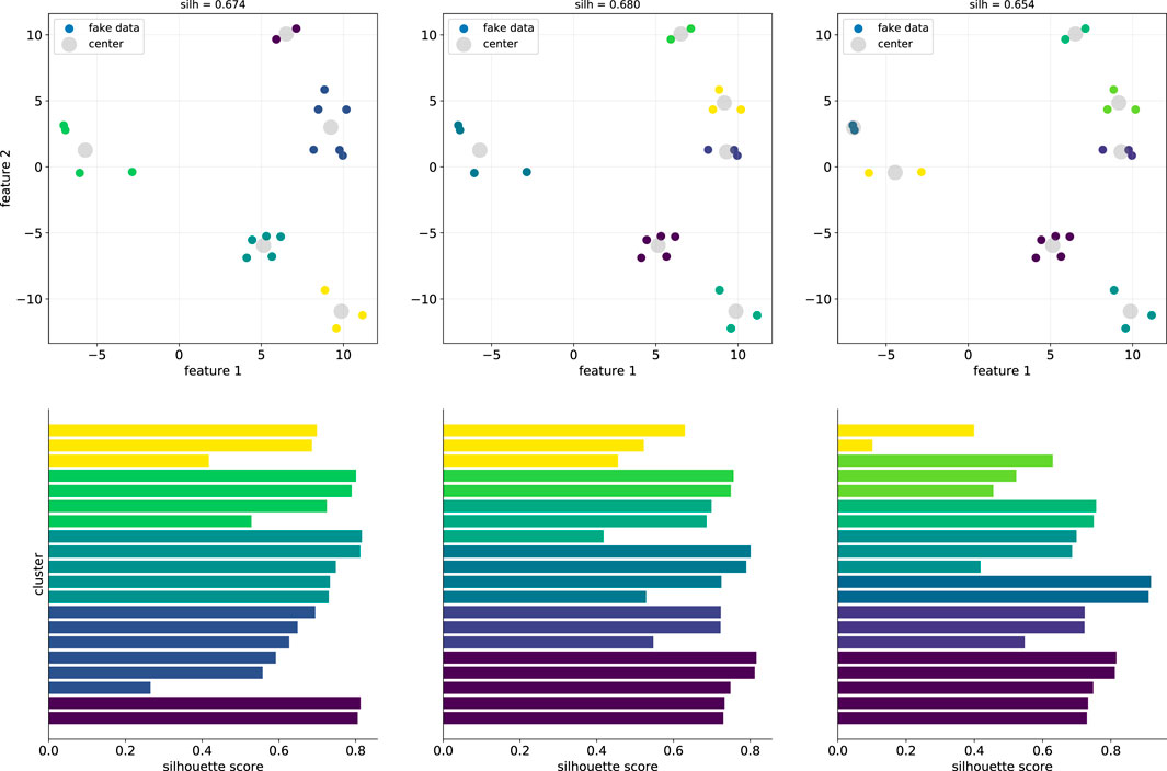
FIGURE 1. Example of forming clusters of three sizes with fake data and generating silhouette scores and diagrams. In the top row, the smaller points are the data points, and the larger gray points are the cluster centers, as determined by k-means. The silhouette score is given at the top of each column; the center column has the highest score. Silhouette diagrams are shown in the diagrams in the bottom row, color coded by the clusters shown in the diagrams above them. Bar lengths are most uniform in the middle column, indicating that none of the points are poorly clustered, and therefore resulting in the middle column’s higher score.
The overall silhouette score is given at the top of each column in Figure 1, and we see that the middle column has a slightly higher score. However, all scores are positive and
2.4 Norms and RBF widths
As mentioned above, RBFs are typically characterized by a scalar distance and a scaling parameter ϵ (See Supplementary Appendix SA for more details). The radial distance r can be defined for multivariate data in terms of the Euclidean distance
Consider the Gaussian RBF
This RBF is unsatisfactory in practice because the components of x contain quantities of different types, scales and units. This suggests that it would be useful to use a weighted norm, which we define as
where W is a matrix that contains the scalings. Choosing a diagonal form for W generalizes (9) to
This is treated by scaling each feature by a “typical” value of that feature; for example, we scale temperatures by 10 eV, densities by 1 g/cc, and nuclear charges by 10, making each scaled feature dimensionless and of order unity. An overall scale remains that is determined by the topology of the data.
Experimental data are rarely aligned along the Cartesian directions of our inputs; as a result, changes in one variable are often correlated with changes in other variables. For example, laser-driven experiments drive shocks that follow the Hugoniot rather than an isochore. For this reason, clusters of points around a center are unlikely to be distributed spherically. The region of influence of the center should reflect the distribution of data points; what is “farther from” or “closer to” the center depends on the topology of the data associated with that center. An extreme example is the case in which a very short-pulse laser is used to heat a sample approximately isochorically: the data lie nearly along a line in parameter space, not as points filling a sphere. We treat these issues by generalizing the distance metric to the Mahalanobis distance
We assume that
Use of the Mahalanobis distance suggests an alternate visualization to the standard silhouette plot in Figure 1. In Figure 2, fake data are again used to find clusters. The dataset is shown with 2–7 clusters. Here, the points are color-coded according to their silhouette value, with darker colors corresponding to lower values. Also shown are contours associated with the covariance matrix of each cluster; these contours indicate each cluster’s orientation and therefore its volume of influence in parameter space. Silhouette scores are shown in the lower right plot, which shows that the choice of four clusters is optimal; when there are more than four clusters, well-isolated clusters are broken into non-isolated subclusters. Importantly, as the number of clusters grows, the region influenced by the data becomes more spherical and suggestive of a single, scalar ϵ. Thus, we anticipate that in the limit of large datasets and large numbers of clusters, the universal function-approximation properties of these anisotropic RBFs will be preserved. Note how dense clusters associated with an unbalanced dataset are assigned to a single center, thereby partially balancing the dataset.

FIGURE 2. A fake dataset separated into two through seven clusters. The color of each data point indicates its silhouette number. The orientation of each cluster is indicated by contours computed from the covariance properties of that cluster, indicating the coverage of the data points in the parameter space. The optimal number of clusters is found using the plot at the lower right that shows the silhouette score versus the number of clusters; the number of clusters with the largest silhouette score is the optimal choice. See Figure 9 for the 3D version using real data.
In summary, the ML approach finds clusters in the data, guided by silhouette scores, finds the covariance of each cluster, uses the covariance as the distance in anisotropic RBFs and learns the discrepancy between
3 Datasets
The approach described above was applied to two datasets, both of which originated from exploding-sample experiments. A dataset that includes the elements Al, Ni, Fe, Cu and W was generated with wires by DeSilva and Katsouros (DK) [25] and has been studied by many authors [34–36]. Conductivities versus temperature, color-coded by density, for these four elements are shown in Figure 3. Another dataset, using wires, foam, tubes, foil and sticks, was generated by Clérouin and co-authors [37] and includes data for the elements Al, Ni, Ti, Cu, Ag, Au, B and Si. The Clérouin et al. data differ from the DK data in two important ways: detailed equations of state were used to connect the energy density to the temperature, and the density was controlled through the use of a fixed-radius ring. Both datasets used here, along with codes used in this work, are available at GitHub [38].
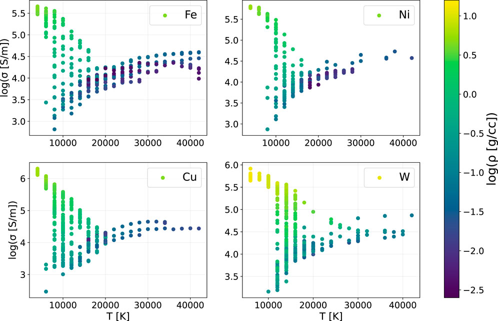
FIGURE 3. DK electrical conductivity data for Fe, Ni, Cu and W. Conductivity is shown versus temperature, with data points color-coded by the mass density. (Conductivity and mass density are shown on logarithmic scales.) Note that the data at high temperatures tend to be at lower densities because of the experimental procedure that employs an exploding wire.
Raw features of these datasets are shown in Figures 4, 5. Variations in and concentrations of values for temperature, density and conductivities are indicated by the histograms along the diagonal. Note that the DK dataset is concentrated at lower temperatures and higher densities, as expected for exploding wires that begin as room-temperature solids. The logarithm of the conductivity is moderately uniform. There are clear trends of conductivity with temperature and density, with the correlation between conductivity and density being slightly stronger than that between conductivity and temperature. While these trends are similar to those seen in the Clérouin data, a key difference is that the Clérouin experiments are very isochoric. (Note that an outlier in the boron data was removed.)
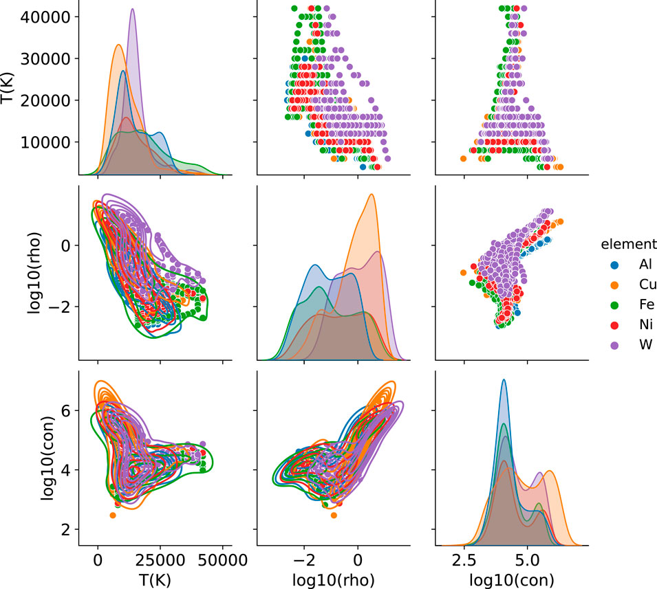
FIGURE 4. DK electrical conductivity data for all five elements (Al, Fe, Ni, Cu and W) shown as histograms and scatter plots. Along the diagonal are the distributions of temperatures (in K), densities (log g/cc) and conductivities (log S/m). Note that some of the data are unbalanced toward lower temperatures or higher densities. Correlations between variables are shown in the off-diagonal plots, which reveal strong correlations between conductivity and density as well as between conductivity and temperature.
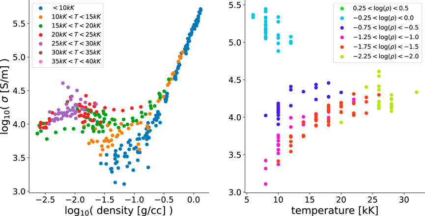
FIGURE 5. Clérouin et al. electrical resistivity data for all elements, shown as histograms and scatter plots. In contrast to the DK data, the densities are constant within a given experiment and resistivities are shown.
We can get a better sense of the physics content of the data by plotting conductivity versus density, with data points color-coded by temperature, and separately, conductivity versus temperature, with data points color-coded by density. These comparisons are shown in Figure 6, where some averaging is done by binning the data into temperature ranges. In the left panel, at low temperatures (blue dots), the conductivity increases monotonically and nearly linearly (in terms of logarithms of the quantities). At elevated temperatures (e.g., orange and green), the conductivity exhibits a minimum, and insufficient data are available to draw a definitive conclusion at the highest temperatures. However, at low densities, there is a trend toward higher conductivities at higher temperatures. This trend is clearer in the panel on the right, where the colors of data points now reflect density bands, with some bands not shown, to reduce clutter. At high densities (shown as green points near the top of the plot), the conductivity drops as the temperature increases. At slightly lower densities (cyan), there is no clear trend. For expanded plasmas, however, the conductivity increases with temperature, a possible signature of a metal-nonmetal transition [36]. Because all of the temperatures in this dataset are below the Fermi energy of Cu (
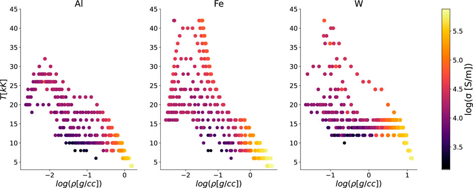
FIGURE 6. The DK data plotted as conductivity versus density (left panel) and versus temperature (right panel) for Al. In the left panel, color coding by temperature reveals strong temperature dependence at low density, with fairly universal behavior at high density. These trends with temperature can be seen in the right panel, in which data points are color-coded by the logarithm of the density: conductivities decrease with temperature at high densities (top, green), are roughly constant at intermediate densities (cyan), and increase with temperature at low densities.
The function we wish to learn is σ(ρ, T). Figure 7 shows the distribution of data points in this input space, color-coded by the conductivity, for three elements: Al, Fe and W. Because this dataset originated from one source—with all data produced using exploding wires—the data do not have well-isolated clusters. Rather, the topology of the data represents the temperature-density path taken by wires with initially high density and low temperature that are heated and expand under pressure. Moreover, because Figure 7 is a 2D projection, we cannot view possible clustering of points along a conductivity axis. Below, we will examine whether our clustering algorithm can find the structure in this dataset.
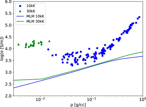
FIGURE 7. Distribution of DK data points in a linear-temperature log-density plane, color-coded by the logarithm of the electrical conductivity, for Al, Fe and W.
4 Results
The modified Lee-More (MLM) model (see Supplementary Appendix SB) is compared with the data in Figure 8 for the two temperatures 10kK and 30kK for a range of densities. This represents an extreme regime—expanded warm dense matter—for the MLM model, and the corresponding errors are clearly visible. Note that the MLM model is used here with no empirical adjustments. The MLM model uses a simple Thomas-Fermi ionization model (see Supplementary Appendix SB) that is not accurate at these low densities and uses a single mean ionization state. Importantly, the MLM model is used here only as the trend
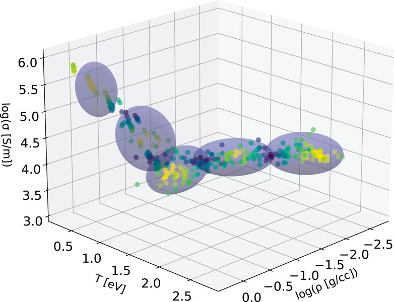
FIGURE 8. Electrical conductivity versus density for the MLM and DK data. Shown are two temperatures, 10kK (blue) and 30 kK (green), for Cu. (To get a sense of the trend in the data, a small band of temperatures around 10kK and 30kK was used).
Next, clustering is used to examine the coverage of the DK data in the density-temperature space, using a cluster analysis. As with most ML methods, the formation of clusters was very sensitive to the data values. Thus, to compress the data onto similar scales, temperatures were scaled by 11,605; that is, temperatures were converted to eV from K. The results are shown in Figure 9.
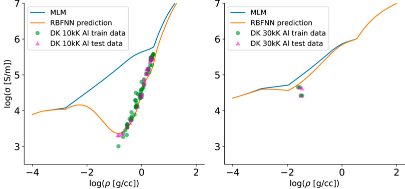
FIGURE 9. Clustering of the DK Al data. As in Figure 2, colors represent silhouette scores; darker points are less well clustered. Note that clusters are formed using all three dimensions (with Z fixed). Five clusters are used, which is two greater than the silhouette score suggested; this increase in cluster number gave an improved prediction.
In practice, once clusters are formed and their covariances are found, three additional steps were performed. First, because the clusters were formed in 3D, a marginal covariance in 2D was found in terms of the input variables x. Second, a hyperparameter was introduced that scales the covariance matrix; physically, this corresponds to learning the region of influence of the data and therefore the scale over which the model reverts to
RBFNN model predictions of Al and Cu electrical conductivity versus density are shown as the orange curves in Figures 10, 11. Because of the large variations in the conductivity values, the logarithm of σ(ρ, T) was used in the learning process. The DK testing data [25] are shown as green points, with testing data chosen randomly from 80% of the total data. Note the agreement of the RBFNN with the data in comparison with the base MLM model and, in particular, how the RBFNN predictions naturally transition to the MLM model predictions away from the data. Here, scale factors of 10 and 30 of the Mahalanobis covariance matrix were used for Al and Cu, respectively, which impacts the widths of the peaks seen in the RBFNN predictions (and therefore the scale over which there is a transition to the MLM model). Because only five centers were used, a high degree of regularization is seen. This is manifested in the good agreement with the green testing data; there is little chance of overfitting with so few centers.
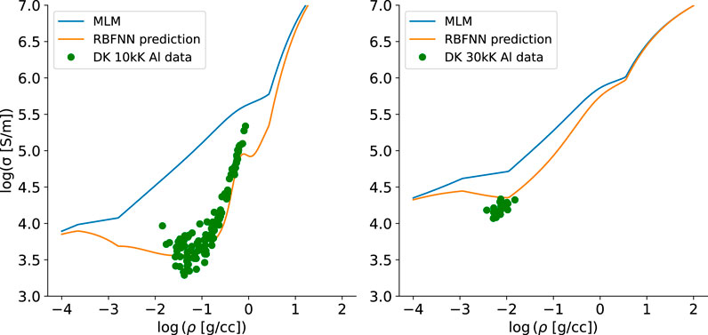
FIGURE 10. DK training data for Al are shown as green dots, with the base MLM model shown as the top, blue curve. The RBFNN model is shown in orange, which predicts the data well and asymptotically (away from the data) tends to the trend
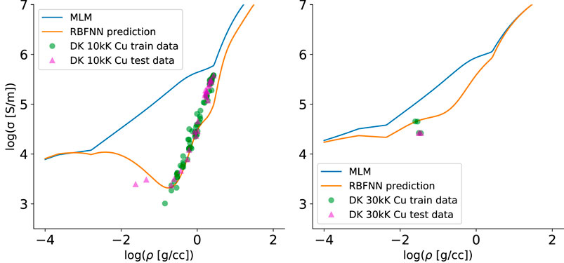
FIGURE 11. DK training data for Cu are shown as green dots, with the base MLM model shown as the top, blue curve. The RBFNN model is shown in orange, which predicts the data well and asymptotically (away from the data) tends to the trend
Next, we turn to the Clérouin et al. dataset. As seen above in Figures 4, 5, the topology of this dataset is very different from that of the DK dataset, and this difference provides an opportunity to further explore the RBFNN approach. Results are shown in Figure 12 for three clusters. Note that the data are nearly constant, with relatively small temperature variations and no density variations; such a topology causes two potential problems not seen with the DK data. First, because the data for each element falls on an isochore, which prevents one from exploring variations along density contours as can be done with the DK data, the lack of variation in density leads to a covariance matrix that has small, and sometimes zero, values. The RBFNN procedure therefore involves singular matrices. These zero values correspond to having no confidence in making a prediction at any density other than the one that was measured. However, if we plot our predictions versus temperature, as in Figure 12, we do not use information for other densities; when the data and predictions are shown this way, a small amount of noise added to the covariance matrix allows for matrix inversion. Second, it is known that RBFNNs are poor at approximating functions that have steps between flat regions, which is how this dataset varies versus temperature. To achieve a sharp transition between flat regions, the RBFNN generates oscillations as seen in the figure.
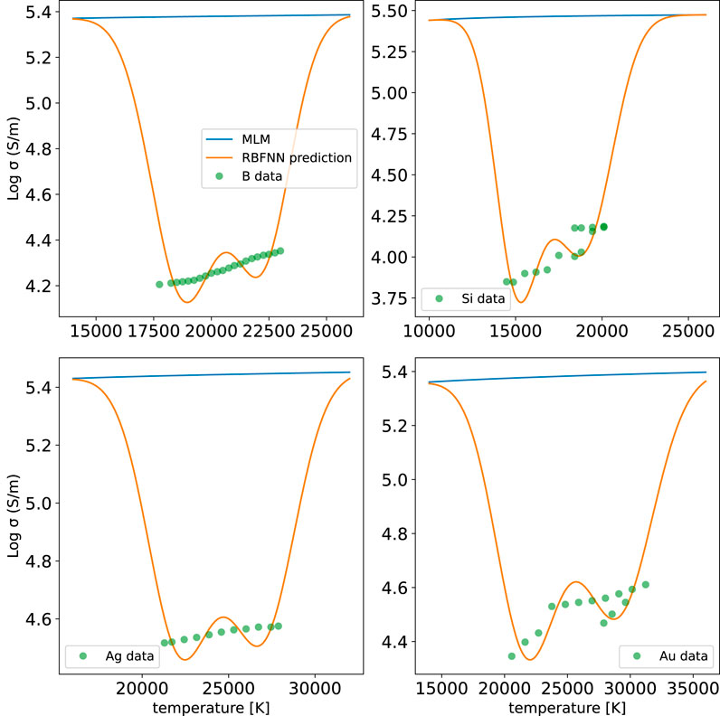
FIGURE 12. Predictions for the Clérouin et al. dataset for four elements. In this case, conductivity is plotted versus temperature because density did not vary within an experiment. Three clusters were used, which limits the ability of the RBFNN to resolve what are nearly flat data.
If we have control over the creation of our data, where should we create it [39]? The Clérouin et al. dataset reveals that, despite the desire to experimentally create well-characterized densities, allowing some variation in density is important from a data-science perspective. (Portions of the Clérouin et al. dataset contained data at two densities for a single element; we leave analysis of these data for future work.) ML methods can be used to guide the creation of datasets [39, 51] that maximize our knowledge with the minimum cost. And, of course, in practice we would combine the datasets; here, these two datasets were kept separate to reveal the interesting differences in their topologies.
5 Conclusion and outlook
In summary, a data-driven approach to predictions of electrical conductivities has been presented. The ML model is based on a detrended RBFNN, where the detrending function
The detrending model
There are many ways that the ML approach can be extended. Chief among them is to enhance the size, quality and sources of the dataset. This can be accomplished by using properties of lower-pressure heated solids and liquid metals, as well as by “computing data” with highly converged, high-fidelity computational models (e.g., Kubo-Greenwood calculations with finite-temperature Kohn-Sham inputs). A topic not discussed here is uncertainty: all discrepancy-learning models [22–24] should be subject to uncertainty quantification and the use of Bayesian methods, such as Gaussian process regression (GPR) [40]. This will be the subject of future work; for example, there are interesting parallels with discrepancy modeling and multifidelity models, many of which are GPR-based [39]. Finally, the approach presented here could be extended to multi-output ML. Simultaneous prediction of multiple electronic transport properties (e.g., including viscosity and thermal conductivity) could enforce consistency among the models. Importantly, a general framework could be constructed that also predicts the equation of state, which allows a more direct use of exploding wire data [26] for which energy density is a more natural independent variable than temperature.
Data availability statement
Publicly available datasets were analyzed in this study. These data can be found here: https://github.com/MurilloGroupMSU/Dense-Plasma-Properties-Database/tree/master/database/DeSilvaKatsouros.
Author contributions
MM conceived and designed the study, performed all calculations and wrote the manuscript.
Acknowledgments
The author thanks A. W. DeSilva for useful conversations. The author is extremely grateful to J. Stephens (Texas Tech University) and S. Hansen (Sandia) for providing DeSilva-Katsouros datasets and to an anonymous referee for providing a CSV file of the Clérouin et al. data. We thank the U.S. Air Force Office of Scientific Research for their support of this work under Grant No. FA9550-17-1-0394.
Conflict of interest
The author declares that the research was conducted in the absence of any commercial or financial relationships that could be construed as a potential conflict of interest.
Publisher’s note
All claims expressed in this article are solely those of the authors and do not necessarily represent those of their affiliated organizations, or those of the publisher, the editors and the reviewers. Any product that may be evaluated in this article, or claim that may be made by its manufacturer, is not guaranteed or endorsed by the publisher.
Supplementary material
The Supplementary Material for this article can be found online at: https://www.frontiersin.org/articles/10.3389/fphy.2022.867990/full#supplementary-material
References
1. Clauser CF, Arista NR. Stopping power of dense plasmas: The collisional method and limitations of the dielectric formalism. Phys Rev E (2018) 97:023202. doi:10.1103/physreve.97.023202
2. Ichimaru S. Statistical plasma physics, volume I: Basic principles. Boca Raton, FL, USA: CRC Press (2018).
3. Pfalzner S, Gibbon P. Direct calculation of inverse-bremsstrahlung absorption in strongly coupled, nonlinearly driven laser plasmas. Phys Rev E (1998) 57:4698–705. doi:10.1103/physreve.57.4698
4. Gaffney J, Hu S, Arnault P, Becker A, Benedict L, Boehly T, et al. A review of equation-of-state models for inertial confinement fusion materials. High Energ Density Phys (2018) 28:7–24. doi:10.1016/j.hedp.2018.08.001
5. Stanton LG, Murillo MS. Ionic transport in high-energy-density matter. Phys Rev E (2016) 93:043203. doi:10.1103/physreve.93.043203
6. Stanton LG, Murillo MS. Efficient model for electronic transport in high energy-density matter. Phys Plasmas (2021) 28:082301. doi:10.1063/5.0048162
7. Grabowski P, Hansen S, Murillo M, Stanton L, Graziani F, Zylstra A, et al. Review of the first charged-particle transport coefficient comparison workshop. High Energ Density Phys (2020) 37:100905. doi:10.1016/j.hedp.2020.100905
8. Wei J, Chu X, Sun X-Y, Xu K, Deng H-X, Chen J, et al. Machine learning in materials science. InfoMat (2019) 1:338–58. doi:10.1002/inf2.12028
9. Barnes BC, Elton DC, Boukouvalas Z, Taylor DE, Mattson WD, Fuge MD, Chung PW. Machine learning of energetic material properties. arXiv preprint arXiv:1807.06156 (2018).
10. Wu Y, Wang H, Zhang B, Du K-L. Neural network implementations for PCA and its extensions. Int Scholarly Res Notices (2012) 2012:847305. doi:10.5402/2012/847305
11. Jain A, Bligaard T. Atomic-position independent descriptor for machine learning of material properties. Phys Rev B (2018) 98:214112. doi:10.1103/physrevb.98.214112
12. Spears BK, Brase J, Bremer P-T, Chen B, Field J, Gaffney J, et al. Deep learning: A guide for practitioners in the physical sciences. Phys Plasmas (2018) 25:080901. doi:10.1063/1.5020791
13. Parsons MS. Interpretation of machine-learning-based disruption models for plasma control. Plasma Phys Control Fusion (2017) 59:085001. doi:10.1088/1361-6587/aa72a3
14. Wang Y, Liao Z, Mathieu S, Bin F, Tu X. Prediction and evaluation of plasma arc reforming of naphthalene using a hybrid machine learning model. J Hazard Mater (2021) 404:123965. doi:10.1016/j.jhazmat.2020.123965
15. Mesbah A, Graves DB. Machine learning for modeling, diagnostics, and control of non-equilibrium plasmas. J Phys D Appl Phys (2019) 52:30LT02. doi:10.1088/1361-6463/ab1f3f
16. Krüger F, Gergs T, Trieschmann J. Machine learning plasma-surface interface for coupling sputtering and gas-phase transport simulations. Plasma Sourc Sci Technol (2019) 28:035002. doi:10.1088/1361-6595/ab0246
17. Gonoskov A, Wallin E, Polovinkin A, Meyerov I. Employing machine learning for theory validation and identification of experimental conditions in laser-plasma physics. Sci Rep (2019) 9:7043. doi:10.1038/s41598-019-43465-3
18. Lee YT, More R. An electron conductivity model for dense plasmas. Phys Fluids (1994) (1984) 27:1273. doi:10.1063/1.864744
19. Rozsnyai BF. Electron scattering in hot/warm plasmas. High Energ Density Phys (2008) 4:64–72. doi:10.1016/j.hedp.2008.01.002
20. Perrot F, Dharma-Wardana M. Electrical resistivity of hot dense plasmas. Phys Rev A (Coll Park) (1987) 36:238–46. doi:10.1103/physreva.36.238
21. Ichimaru S, Tanaka S. Theory of interparticle correlations in dense, high-temperature plasmas. V. Electric and thermal conductivities. Phys Rev A (Coll Park) (1985) 32:1790–8. doi:10.1103/physreva.32.1790
22. Yang C, Zhang Y. Delta machine learning to improve scoring-ranking-screening performances of protein—ligand scoring functions. J Chem Inf Model (2022) 62:2696–712. doi:10.1021/acs.jcim.2c00485
23. Lu J, Hou X, Wang C, Zhang Y. Incorporating explicit water molecules and ligandconformation stability in machine-learning scoring functions. J Chem Inf Model (2019) 59 (11):4540–49.
24. Kaheman K, Kaiser E, Strom B, Kutz JN, Brunton SL. Learning discrepancy models from experimental data. arXiv preprint arXiv:1909.08574.
25. DeSilva A, Katsouros J. Electrical conductivity of dense copper and aluminum plasmas. Phys Rev E (1998) 57:5945–51. doi:10.1103/physreve.57.5945
26. DeSilva AW, Vunni GB. Electrical conductivity of dense Al, Ti, Fe, Ni, Cu, Mo, Ta, and W plasmas. Phys Rev E (2011) 83:037402. doi:10.1103/physreve.83.037402
27. Bemporad A. Global optimization via inverse distance weighting and radial basis functions. Comput Optim Appl (2020) 77:571–95. doi:10.1007/s10589-020-00215-w
28. Specht DF. A general regression neural network. IEEE Trans Neural Netw (1991) 2:568–76. doi:10.1109/72.97934
29. Jain AK, Murty MN, Flynn PJ. Data clustering. ACM Comput Surv (1999) 31:264–323. doi:10.1145/331499.331504
30. Rokach L, Maimon O. Data mining and knowledge discovery handbook. Berlin, Germany: Springer (2005). p. 321–52.
31. Tarekegn AN, Michalak K, Giacobini M. Cross-validation approach to evaluate clustering algorithms: An experimental study using multi-label datasets. SN Comput Sci (2020) 1:263. doi:10.1007/s42979-020-00283-z
32. Fayyad U, Piatetsky-Shapiro G, Smyth P. From data mining to knowledge discovery in databases. AI Mag (1996) 17(3):37. doi:10.1609/aimag.v17i3.1230
33. Rousseeuw PJ. Silhouettes: A graphical aid to the interpretation and validation of cluster analysis. J Comput Appl Math (1987) 20:53–65. doi:10.1016/0377-0427(87)90125-7
34. Zaghloul MR. Erratum: “A simple theoretical approach to calculate the electrical conductivity of nonideal copper plasma” [phys. Plasmas 15, 042705 (2008)]. Phys Plasmas (2008) 15:109901. doi:10.1063/1.2996112
35. Stephens J, Dickens J, Neuber A. Semiempirical wide-range conductivity model with exploding wire verification. Phys Rev E (2014) 89:053102. doi:10.1103/physreve.89.053102
36. Clérouin J, Renaudin P, Laudernet Y, Noiret P, Desjarlais MP. Electrical conductivity and equation-of-state study of warm dense copper: Measurements and quantum molecular dynamics calculations. Phys Rev B (2005) 71:064203. doi:10.1103/physrevb.71.064203
37. Clérouin J, Noiret P, Blottiau P, Recoules V, Siberchicot B, Renaudin P, et al. A database for equations of state and resistivities measurements in the warm dense matter regime. J Plasma Phys (2012) 19 (8):082702.
38. Murillo MS. DeSilva and Katsouros Cu data (2022). Available from: https://github.com/MurilloGroupMSU/Dense-Plasma-Properties-Database/tree/master/database/DeSilvaKatsouros.
39. Stanek LJ, Bopardikar SD, Murillo MS. Multifidelity regression of sparse plasma transport data available in disparate physical regimes. Phys Rev E (2021) 104:065303. doi:10.1103/physreve.104.065303
41. Park J, Sandberg IW. Universal approximation using radial-basis-function networks. Neural Comput (1991) 3:246–57. doi:10.1162/neco.1991.3.2.246
42. Poggio T, Girosi F. Networks for approximation and learning. Proc IEEE (1990) 78:1481–97. doi:10.1109/5.58326
43. Broomhead DS, Lowe D. Radial basis functions, multi-variable functional interpolation and adaptive networks. In: Tech. Rep. Malvern, United Kingdom: Royal Signals and Radar Establishment (1988).
44. Murillo MS. Strongly coupled plasma physics and high energy-density matter. Phys Plasmas (2004) 11:2964–71. doi:10.1063/1.1652853
45.The notation ϵ was chosen for the width parameter for consistency with the library sci-kit learn, which was used for these results.
46. Moody J, Darken CJ. Fast learning in networks of locally-tuned processing units. Neural Comput (1989) 1:281–94. doi:10.1162/neco.1989.1.2.281
47. Bugmann G. Normalized Gaussian radial basis function networks. Neurocomputing (1998) 20:97–110. doi:10.1016/s0925-2312(98)00027-7
50. Schløler H, Hartmann U. Mapping neural network derived from the parzen window estimator. Neural Networks (1992) 5:903–9. doi:10.1016/s0893-6080(05)80086-3
51.These results were obtained using the scikit-learn library, which uses the parameter α to characterize regularization. Although its default kernel is linear, the Gaussian has been used here.
52. Stanton LG, Glosli JN, Murillo MS. Multiscale molecular dynamics model for heterogeneous charged systems. Phys Rev X (2018) 8:021044. doi:10.1103/physrevx.8.021044
53. Goano M. Series expansion of the Fermi-Dirac integral over the entire domain of real j and x. Solid-State Electron (1993) 36:217–21. doi:10.1016/0038-1101(93)90143-e
54. Stanton L, Murillo M. Publisher's Note: Unified description of linear screening in dense plasmas [Phys. Rev. E 91, 033104 (2015)]. Phys Rev E (2015) 91:049901. doi:10.1103/physreve.91.049901
Keywords: machine learning, electrical conductivity, plasma transport, warm dense matter, dense plasma
Citation: Murillo MS (2022) Data-driven electrical conductivities of dense plasmas. Front. Phys. 10:867990. doi: 10.3389/fphy.2022.867990
Received: 01 February 2022; Accepted: 25 August 2022;
Published: 24 November 2022.
Edited by:
Mianzhen Mo, Stanford University, United StatesReviewed by:
Zheng Li, Peking University, ChinaTianyu Guo, Peking University, China and Jingcheng Hu, Zhejiang University, China, in collaboration with reviewer ZL
Nathaniel Shaffer, University of Rochester, United States
Copyright © 2022 Murillo. This is an open-access article distributed under the terms of the Creative Commons Attribution License (CC BY). The use, distribution or reproduction in other forums is permitted, provided the original author(s) and the copyright owner(s) are credited and that the original publication in this journal is cited, in accordance with accepted academic practice. No use, distribution or reproduction is permitted which does not comply with these terms.
*Correspondence: Michael S. Murillo, murillom@msu.edu