Effects from dayside magnetosphere to distant tail unleashed by a bifurcated, non-reconnecting interplanetary current sheet

Introduction

The terrestrial magnetosphere constitutes an obstacle to the continuous flow of magnetized plasma from the Sun, i.e., the solar wind, and its dynamics derive in large measure from its interactions with this stream. The solar wind flowing past the magnetosphere changes over various timescales. From a geoeffectiveness perspective, variations on long time scales have attracted most attention, specifically those associated with interplanetary coronal mass ejections (ICMEs) and, in particular, their subset magnetic clouds (MCs [1]). In these large (fraction of an AU) solar eruptions, important parameters, such as the North-South component of the magnetic field, Bz, change slowly and can reach extreme values not otherwise sampled and which are maintained for several hours, even days. This continued forcing of the magnetosphere gives rise to geomagnetic storms of a wide range of intensities (e.g., [2,3]), and repetitive substorm activity [4,5], such as sawtooth events (e.g., [6]).

The solar wind also changes in a discontinuous fashion. Such transient changes can occur, for example, at tangential (TDs) and rotational (RDs) discontinuities [7–9], and shocks. Studies of the impact that these directional discontinuities (DDs) have on the coupled magnetosphere-ionosphere (M-I) system have been by nature more eclectic and, in some sense, more interesting. There are various reasons for this. Among them are: 1) while impulsive at source, they can set in motion a chain of interlinked responses mediated by field-aligned currents (FACs) which couple momentum and energy from the magnetosphere to the ionosphere; 2) waves that typically accompany a strong disturbance of a magnetoplasma propagate and spread out, transmitting the effects and, importantly, 3) DDs are very frequent in the solar wind. Further, the impulsive changes may involve more than one parameter. Even for DDs involving just the magnetic field vector, one has to take into account the different background plasma and field conditions they occur in (e.g., a North-South deflection of a strong magnetic field in a tenuous plasma). Also, shocks may be isolated or may be driven by CMEs and high-speed streams in corotating interaction regions (CIRs), or may be propagating inside a CME. In the last case, for example, the disturbances of magnetospheric plasmas and fields can be very strong: thus, in two studied cases they emptied the outer radiation belt of energetic electrons (see e.g., [10,11]).

Although of short duration at source, the effects of DDs on magnetospheric plasmas and fields can be spread out in time. Intuitively, the strength of the response should depend on the amplitude of the impulsive change, at least until saturation, if there is any, sets in. Combinations of simultaneous impulsive changes introduce additional features in the magnetospheric response. For example, sharp velocity deflections accompanying the magnetic changes at a TD usher in a vortex sheet element and the latter results in tangential stresses being exerted on the magnetopause (see, e.g., [12]). A TD at which there is a sharp rise/drop in density will undergo a change as it interacts with the bow shock. Thus, for a density rise a fast magnetosonic wave carrying part of the density jump precedes the modified TD and perturbs the magnetopause first [13,14]. This was realized in a prescient study by [15] (see also [16]), and shown observationally by [17] and [18]. In addition, a pressure rise at a TD which is oriented such that the motive electric field points towards it from at least one side can excite hot flow anomalies (HFA) at the bow shock which may lead to a distortion of the magnetopause in the form of a local protrusion [19–21] and large-amplitude motions. HFAs illustrate the point that while transient changes in the interplanetary (IP) medium may seem fairly innocuous, they may yet trigger considerable disturbances in the magnetospheric plasmas and fields.

In what follows we shall examine such a case. Our focus is on a short-duration (∼1/2 h) variation in the interplanetary plasma and magnetic field parameters which we identify as a current sheet (CS). Absence of accelerated flows indicates it is non-reconnecting. Through a very good deployment of spacecraft we can monitor its effects on the magnetosheath/magnetosphere, from dayside to the far tail (∼−230 Re). Its effects are found to be clear and large. In particular, a large flux rope structure was ejected down the distant tail at great speed before a tail flapping episode began. Interestingly, the IP feature is embedded in a long (∼1 day) ICME which provides the ambient medium our feature occurs in. This ambient medium is marked by large non-radial flows and strong fields whose effects on the dayside, duskside magnetosheath and in the far tail (windsock-type deflection and twisting) are clearly seen.

We make use of the following data sets. From the Advanced Composition Explorer (ACE) we analyze magnetic field data from the Magnetic Field Experiment (MAG [22]) and proton data from the Solar Wind Electron Proton Alpha Monitor (SWEPAM [23]) at 16 s (occasionally, 1 s) and 64 s resolution, respectively. Data from Wind are provided by the Magnetic Fields Instrument (MFI [24]) and the 3DP instrument (3DP [25]). Typically, we use data at 3 s resolution from both. The Wind 3DP instrument consists of six different sensors. There are two electron (EESA) and two ion (PESA) electrostatic analyzers with different geometrical factors and field-of-views covering the energy range from 3 eV to 30 keV. More details can be found in [26], who also review 20 years of discoveries made by Wind. Geotail magnetic and plasma data are from the MGF [27] and LEP [28] instruments, respectively, at a resolution of 3 s (MGF) and 12 s (LEP). Cluster magnetic field data are from the Cluster Magnetic Field investigation (MGF [29]), and the plasma data are from the Cluster Ion Spectrometry experiment (CIS [30]). Polar magnetic field data are from the Magnetic Fields Experiment (MFE [31]) and plasma data are from the hot plasma Analyzer (HYDRA [32]). Key parameters at 1 min and 6 s resolution are employed. Defense Meteorological Satellite Program (DMSP) satellites are Sun-synchronous satellites in nearly circular polar orbit at an altitude of roughly 835 km and an orbital period of approximately 101 min. The SSJ instrument package included on all recent DMSP flights uses curved plate electrostatic analyzers to measure ions and electrons from 30 eV to 30 keV in logarithmically spaced steps [33]. Because of its upward pointing and limited pitch angle resolution, DMSP SSJ measures only highly field-aligned precipitating particles. The DMSP magnetic field experiments (SSM) consist of triaxial fluxgate magnetometers with a range of ± 65,535 nT and one-bit resolution of 2 nT [34]. The time resolution of SSJ and SSM data is 1 s. The DMSP magnetic field data can provide estimates of the large-scale structure of FACs (e.g., [35–37]).

Interplanetary and far tail observations

Interplanetary observations are from spacecraft ACE in orbit around the L1 point. Before we describe them, we present an overview of the effect in the far tail which motivated this investigation. It was observed by the spacecraft Wind which was sampling the distant tail near the ecliptic plane on the duskside.

Figure 1 shows Wind plasma and magnetic field observations over a 2-h interval from 11 to 13 UT on 10 January 2004. During this interval Wind was near the Earth-Sun L2 point in the geomagnetic tail at an average position vector R = (−227, 34, −9) R_E (GSE), i.e., on the duskside and slightly south of the ecliptic. From ∼11:30 to ∼11:55 UT, the Earth-Sun Bx component repeatedly changed polarity (panel 4), i.e., the tail was flapping. But before the flapping, there is a different structure, a “precursor”, shown between vertical guidelines. Here the density is low, and the temperature is high. The total magnetic field, B, is enhanced, and the field components rotate through a large angle. As shown later, the field change is embedded in a plasma flow which is strongly tailward. This feature is the focus of our paper: What gave rise to it and what perturbations did it excite in the magnetosphere?

FIGURE 1

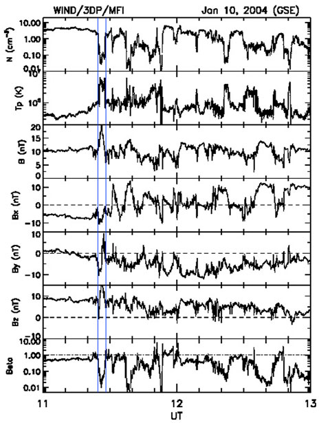
FIGURE 1. Proton and magnetic field data from spacecraft Wind during 11–13 UT, 10 January 2004. From top to bottom: the proton density, temperature, total field and its GSE components, and the proton beta.

We have not yet included plasma velocities. This is because the bulk velocities from the PESA Low instrument are not trustworthy during this period. They follow the proper trends but are not to be trusted in absolute values. We shall return to this qualification when later we use moments from the analysis of the full 3D velocity distribution functions (VDFs) from PESA High, as we discuss Wind observations in more detail.

We return to ACE observations. Figure 2 shows 1 day of data. This is a tabulated, fast ICME lasting from six UT, January 10 to 5 UT, 11 Jan 2004 [38]. Some relevant features are as follows:

1) There are strong non-radial flows, particularly in Vy. This is unusual for ICMEs (see [39]). In accordance with the windsock effect, we expect a deflected tail [40–43].

2) Close to the red vertical guideline at ∼10:10 UT, there are clear field and flow gradient discontinuities near maximum B. These give the temporal profiles of the field and flow a “kink-like” structure. (In this context, by “kink” we mean a place where there is a discontinuous change in the temporal gradients of B and V.) This is our focus. There is a strong By component, whose gradient changes at the red line. A short time earlier the Vy component transitions from negative to positive values. Torques are being applied to the tail which twist it [20,44,45].

3) At this structure, there is a peak in the density concomitant with a decrease of 20% of a strong B. This will serve as a good tracer when we look at observations from other widely-spread spacecraft.

4) The structure lies in a ∼4-hour-long region of strong and positive GSM Bz. During this, the clock angle (i.e., the polar angle in the GSM YZ plane; last panel) is less than 60^°.

FIGURE 2

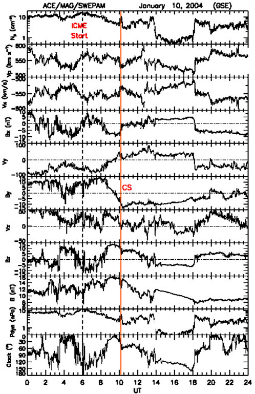
FIGURE 2. ACE observations on 10 January 2004. From top to bottom: the proton density, bulk speed, (pairwise) components of flow and magnetic field, the dynamic pressure in nPa, and the IMF clock angle, i.e., the polar angle in the GSM YZ plane. The dynamic pressure includes the alpha-particle contribution. The vertical red line shows the time of the current sheet which we discuss here.

In summary, while compared to the larger ICME structure these features look innocuous enough, their effects are significant. In addition, we shall also show that they are related to the precursor at Wind.

A shorter interval is plotted in Figure 3. The resolution of the magnetic field data is now 1 s. The feature lasts for ∼17 min. The dynamic pressure (top panel, blue trace) shows a 2-pronged profile: it rises (from 2 to 4.8 nPa), drops (to 3.2 nPa), rises again (to 6 nPa) and then decreases to ambient values (2 nPa). This will cause the magnetopause to bounce. We performed a minimum variance analysis on the 1-s magnetic field data in the interval 10:00–10:25 UT. The routine returned a normal, N = (0.77, 0.50, 0.38) (GSE). The intermediate-to-minimum eigenvalue ratio = 3.3. We thus have a CS. There was a normal field component, B_N = −4.52 ± 0.59 nT. The CS is bifurcated, with sharp changes at the edges, and a plateau in between. There is no plasma jetting, so that it is a non-reconnecting CS. There is indication that minimum B precedes the strongest rise in Np by about 5 min.

FIGURE 3

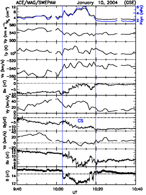
FIGURE 3. A zoom-in of the interval 9:40–10:40 UT. The ACE field data are now at a resolution of 1 s. The vertical blue lines bracket the CS. Overlaid on the density in the top panel is the dynamic pressure (in blue, with scale on the right). Note that the minimum in B (bottom panel) occurs ∼5 min before the density reaches its peak value.

Figure 4 shows the positions of the spacecraft, with on the left the XY GSE plane and on the right the ZX plane. The top panel shows ACE at the L1 point (red) and Wind (blue) at the L2 point in the distant tail. The spacecraft separation in X is ∼480 R_E. The bottom panel shows the positions of Geotail (blue), Cluster 1 (red) and Polar (purple). Geotail is in the ecliptic plane at dawn magnetic local times (MLTs). Cluster 1 and Polar are at dusk South of ecliptic. Cluster 1 is near the bow shock and Polar is initially inside the magnetosphere. We thus have satellites providing simultaneous observations from all important regions: unperturbed solar wind, near the magnetopause, just below the magnetopause, and at the distant tail.

FIGURE 4

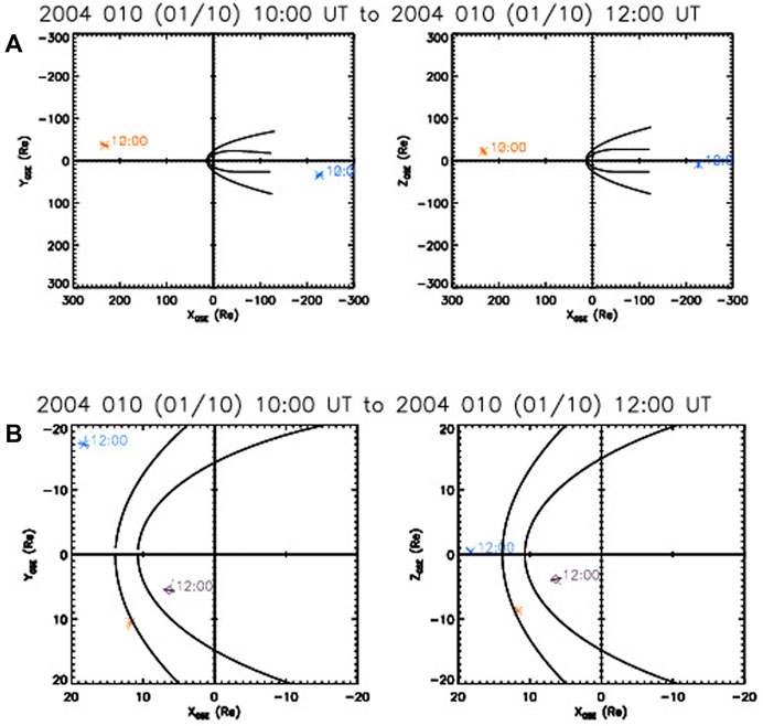
FIGURE 4. The positions of the spacecraft at 11 UT. (A) (top): ACE (red) upstream of Earth near the L1 point and Wind (blue) in the distant tail. (B) (bottom): The near-magnetopause spacecraft: blue: Geotail, red: Cluster 1, purple: Polar. The left-hand panels show the XY GSE plane while those on the right hand show the XZ GSE plane. The curves show model bow shock and magnetopause

Observations near the dayside magnetopause and bow shock

We discuss observations near the dayside magnetopause and bow shock made by Geotail, Cluster 1 and Polar. Figure 5 shows an overlay of ACE (black trace) and Geotail (blue trace) magnetic field data at 16 and 3 s resolution, respectively. The CS arrives at Geotail at ∼10:50 UT. The agreement is very good when the ACE data are shifted forward in time by 46 min. Correlation coefficients are: 0.93 (Bx), 0.98 (By), and 0.92 (Bz). We conclude that Geotail remained in the solar wind all the time. The remarkable agreement implies that the CS is not evolving much while traveling in the solar wind from ACE to GT, which are separated by 217.0 R_E, mostly in the X-direction.

FIGURE 5

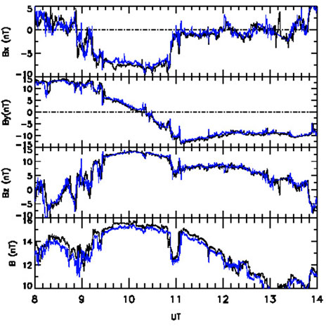
FIGURE 5. An overlay of ACE (black) and Geotail (blue) magnetic field data. ACE data are delayed by 46 min.

Next, we turn to Cluster 1. We recall that Cluster 1 was expected to be in the Southern hemisphere near the bow shock (Figure 4). Figure 6A gives an overlay of ACE (black trace) and Cluster 1 (red) data for the 10-h interval 6 to 16 UT. Delaying ACE data by 47 min results in very good agreement when Cluster 1 is in the solar wind (up to ∼11:10 UT), similar to that between ACE and Geotail. Thus, the CS arrives at Cluster 1 and Geotail practically simultaneously. Performing a minimum variance analysis on the Geotail magnetic field data in the interval 10:40–11:20 UT, we obtain a normal (GSE) N = (0.75, 0.29, 0.60) (eigenvalue ratio = 8.6). Thus, the CS will arrive at the duskside magnetopause first.

FIGURE 6

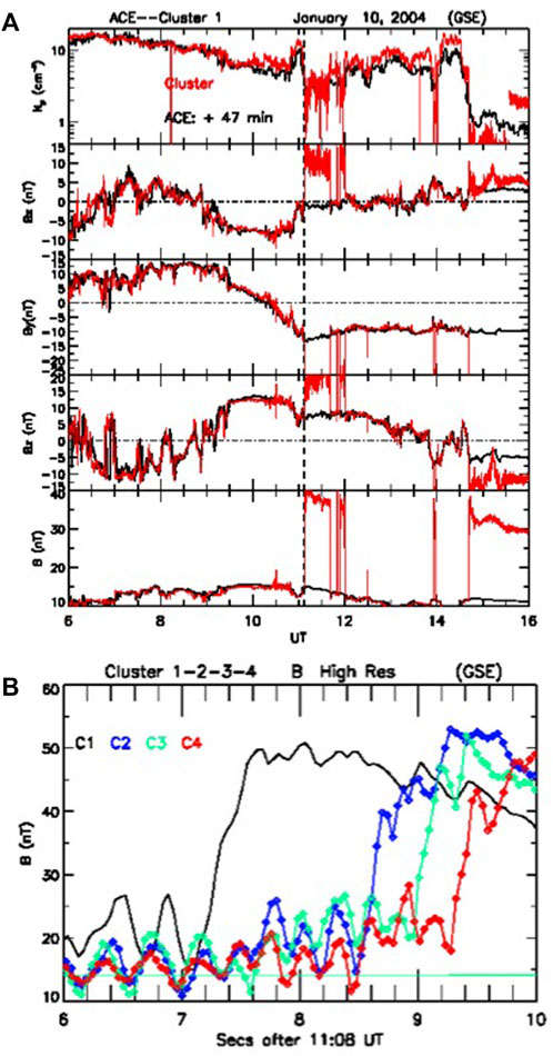
FIGURE 6. (A) (top). Overlay of ACE (black) and Cluster 1 (red) data for the interval 6 to 16 UT. ACE data have been delayed by 47 min. (B) (bottom): The crossing of the bow shock by the four Cluster spacecraft.

As the dynamic pressure decreases just after the B-drop at the CS, Cluster 1 crosses the sunward—moving bow shock into the magnetosheath. The outward motion of the bow shock can be studied by timing its passage over the Cluster configuration. The four spacecraft enter the magnetosheath in the order C1-C2-C3-C4. Shown in Figure 6B is a clear rise in B observed by all the spacecraft just after 11:08 UT. We triangulate this feature using the technique of [46], [47]. Four-spacecraft timing gives a bow shock velocity along its normal of V = 98.6*(0.9, 0.2, −0.3) km/s, i.e., sunward, duskward and southward.

We now consider Polar observations. At 11 UT, the spacecraft was at (6.1, 4.8, -4.2) R_E (GSE), i.e., on the duskside south of the ecliptic. Figure 7 shows magnetic field and electron data. (Proton data from HYDRA are not available.) From top to bottom, the figure shows the electron density, bulk speed and temperature at 14 s temporal resolution, the magnetic field components in GSE coordinates, and the total magnetic field. The resolution of the magnetic field data is 0.92 min. For the 17-min interval 10:51 to 11:08 UT (between vertical guidelines), the temporal profile of Ne closely resembles that at Cluster 1 and ACE. Timing the arrival of the density peak, we find a delay ACE-Polar of ∼48 min. The high-density structure is associated with a decrease in electron flow velocity, and reduced temperatures. There is a 2-pronged drop in the magnetic field strength, the second of which coincides with the density rise.

FIGURE 7

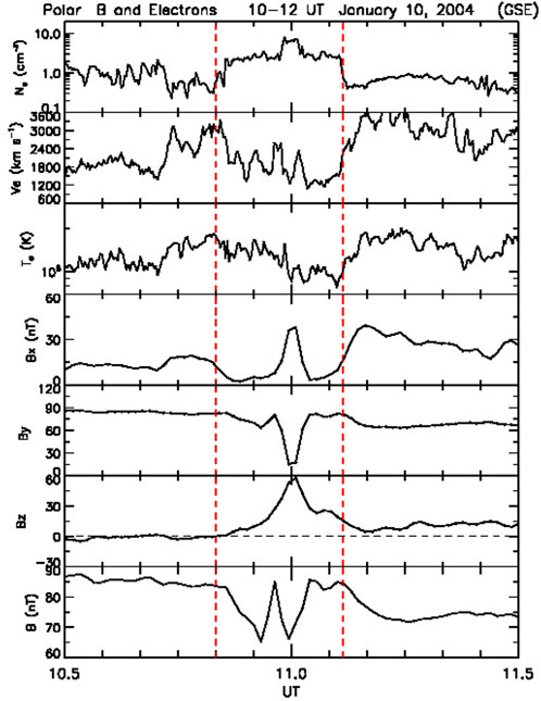
FIGURE 7. Data from the MFE and HYDRA instruments on Polar. Electron data: density, bulk speed and temperature. Magnetic field: Components in GSE coordinates and total field. The vertical guidelines bracket the interval where the clear changes in all these parameters suggest that Polar is sampling the CS-structure observed about 48 min earlier by ACE.

To better understand what Polar is seeing, we consider the effect of the CS when it is near the duskside magnetopause. Recall that Cluster 1 and Polar are on the duskside at a distance of 9.4 R_E and on opposite sides of the magnetosheath (Figure 4), so the effect on the immediate neighborhood of Polar can be monitored well. Shown in Figure 8 are the data from Polar and Cluster 1 (in blue) around the time when the CS reached Cluster 1, whose data have been shifted by 1.5 min to align the peaks of the density profiles.

FIGURE 8

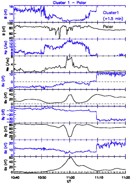
FIGURE 8. Polar (black traces) and Cluster 1 (blue) for the interval 10:40—11:20 UT. Cluster 1 data have been time-shifted by 1.5 min to align the peaks of the density profiles in panels 3 and 4.

Clearly, the two spacecraft see very different magnetic field profiles. Because the CS is also associated with (large) changes in the velocity, there is a vortex sheet element involved, and the structure will exert tangential stresses in addition to normal ones (see [12]). These will distort the magnetopause. We now show that the tangential stresses are comparable to the normal ones by considering the pressure tensor.

The total pressure tensor (total momentum flux tensor) is given by

${\mathrm{\Pi }}_{\mathrm{a}\mathrm{b}}=\left(p+B^2/2{\mu }_0\right){\delta }_{ab}+\rho V_a{V}_b-B_a{B}_b/{\mu }_0$

where a, b are running indices over the (i, j, k) coordinates resulting from MVAB, p is the thermal plasma pressure, and ρ is the mass density. MVAB analysis on the Cluster 1 data for the interval 10:48 to 11:08 UT gave the following eigenvalues i = (−0.58, 0.81, −0.11), j = (−0.24, −0.046, 0.97), and k = (0.78, 0.59, 0.22). The intermediate-to-minimum eigenvalue ratio = 13.0, so the result is robust. The result is shown in Figure 9. The tangential stresses (third and fourth panels) are even somewhat larger than the normal ones (panel 2). Thus, on transmission through the bow shock, we expect a strong local deformation of the magnetopause and perturbations in the magnetosheath [17,48].

FIGURE 9

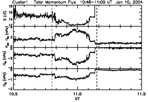
FIGURE 9. The pressure tensor based on Cluster 1 spacecraft data. From top to bottom, the total field for reference, the total pressure in the direction perpendicular to the CS at Cluster 1, ∏_kk, and the tangential stresses in the ith (∏_ki) and jth directions (∏_kj).

Indeed, in Figure 8, around 11 UT when Polar sees a density enhancement, By goes from ∼90 to ∼0 nT and Bz goes from 0 to 60 nT. These values are different from those recorded by the spacecraft while in the magnetosphere at the beginning and end of the interval plotted. Thus, Polar is probably crossing briefly into the magnetosheath, which is strongly disturbed and deformed by the forces exerted on it by the CS, which resulted in this field rotation.

Figure 10 shows differential energy fluxes of electrons and ions. From 10:50 to 11:06 UT there is a clear enhancement in both, when Polar is sampling the passage of the density peak in the CS structure. A 2-dip structure in B (Figure 7) is seen due to the 2-dip profile of Pdyn at ACE (Figure 3).

FIGURE 10

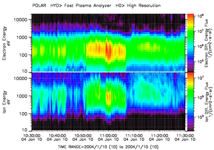
FIGURE 10. Polar/HYDRA differential energy fluxes, with electrons at the top and ions at the bottom. At 11 UT Polar is sampling the SC-structure while located at the distorted magnetosphere/magnetosheath boundary.

Observations from low-altitude spacecraft

We next consider observations from the low-altitude spacecraft F16 and F13, which were following dawn-to-dusk trajectories in the Southern hemisphere, rising to about 80° MLAT. Figure 11 shows, from top to bottom, the energy fluxes of electrons and ions, the density, the velocity and the magnetic field perturbations seen by F16 from 10:39 to 11:09 UT. We supplement this with the top part of Figure 12 (Figure 12A), which shows the magnetic field, and the electron and ion spectrograms. The MLAT and MLT are given at bottom. Around 10:59:02 UT (similar time to Polar) during the bouncing motion of the magnetopause and when F16 was at the poleward edge of the oval, the spacecraft sees a strong (∼3 km/s) sunward flow burst in a double vortex-like structure (Figure 11, fourth panel). From Figure 12A, which plots more clearly the cross-track (green solid line) and along-track (magenta dotted line) perturbations in the magnetic field, this flow structure is flanked by two (up and down) field-aligned currents (FACs), which change polarity at ∼11 UT.

FIGURE 11

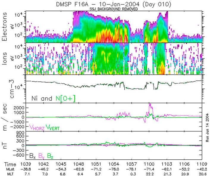
FIGURE 11. Satellite F16 field and plasma data collected on a dawn-dusk pass reaching to high MLATs in the Southern hemisphere. The focus is on the sunward-directed, 3 km/s flow burst at around 11 UT (panel 4). For further details, see text.

FIGURE 12

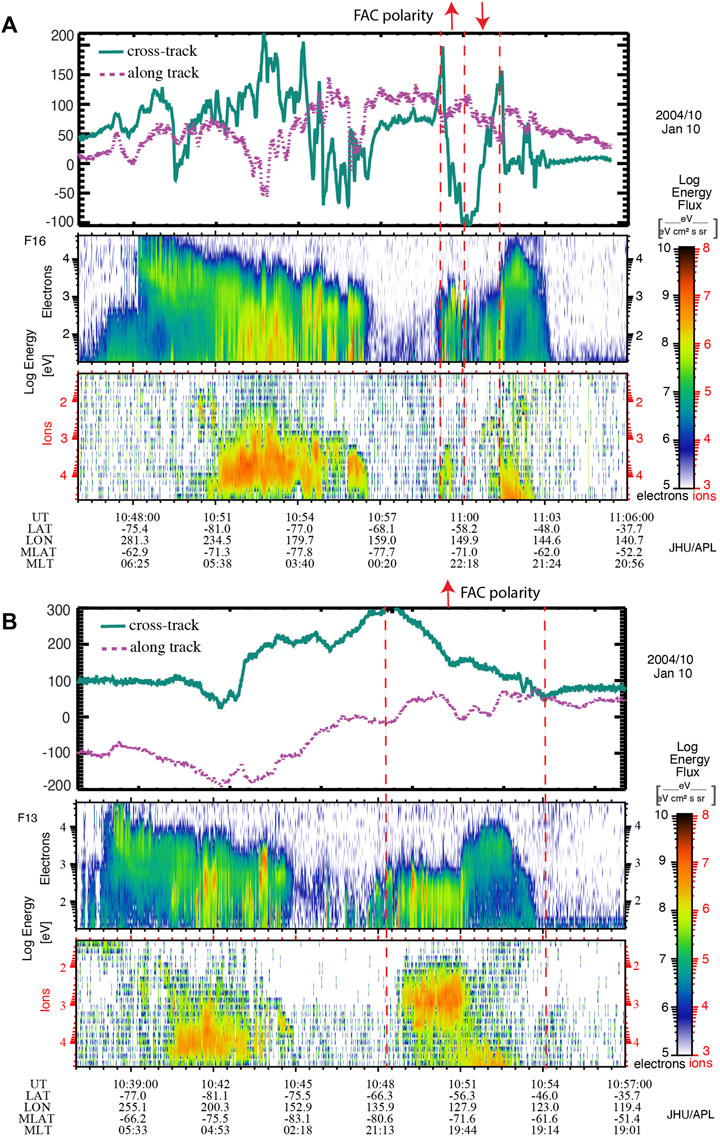
FIGURE 12. (A) (top) A zoom-in of F16 data showing the magnetic field perturbations and associated FAC pair, and the precipitation electrons and ions they occur in. (B) (bottom) Similar observations made by F13 in the southern hemisphere in approximately the same region as F16 but about 1–2 h MLT earlier. It is included to put the F16 observations into context.

In the poleward region of the oval at pre-midnight local times (MLT = 21:48–22:47), the FAC is upward a few min before 11:00 UT and then downward a few min after 11:00 UT. In the upward FAC region, mono-energetic and broadband electrons can be found [49,50]. As discussed next, the equatorward portion of the oval at pre-midnight (MLT ∼21:48–21:22 and MLAT ∼ −67.0° to −61.4°) is sampled at 11:01:23–11:03:11 UT and the precipitation looks more typical, suggesting that closer to Earth, near the isotropy earthward boundary, the behavior of plasma and magnetic field is more typical. At post-midnight (00:30–05:00 MLT), at the poleward region of the oval, there is evidence of broadband electron acceleration which can be attributed to Alfvén wave activities (e.g., [49]).

Figure 12B, which shows the magnetic field and spectrograms from F13, is included for context. F13 crosses almost the same region as F16 but about 10 min earlier and 1–2 h earlier in MLT. This gives us an idea what the region looked like before the disturbance. Prior to 11:00 UT, the postmidnight-dawn auroral oval looks very similar in F13 and F16 and exhibits typical, moderately active plasma sheet and plasma sheet boundary layer (PSBL) electron and ion precipitation (e.g., [51]; [52]). F13 crosses the premidnight oval from 10:47:44 to 10:53:48 UT, prior to the arrival of the disturbance, and also observes typical moderately active plasma sheet precipitation. The first panel in Figure 12B shows that F13 also observes region-1 (R1) upward FAC (e.g., [37]). However, when F16 crosses the pre-midnight oval about 10 min later the characteristics of the oval had changed, particularly the poleward portion of the auroral oval where the spacecraft observes up and down FAC regions and reduced electron and ion precipitation energy fluxes, as described above. On the other hand, the equatorward portion of the oval at 11:01:23—11:03:11 UT (MLAT = –67.01° to –61.41°) looks similar to that observed by F13.

Far tail observations

We now return to the prime concern which kicked off this investigation: Wind’s observation of a precursor to tail flapping (Figure 1). A close view of this “precursor” is given in Figure 13. For the 10-min interval 11:20 to 11:30 UT, this plot shows the proton density, temperature and flow components in GSE coordinates, the total field and its GSE components, and the proton ß. Since, as noted earlier, the absolute values of the velocity moments derived from the onboard moments of the PESA Low instrument are not to be trusted, we use PESA High, at a resolution of ∼90 s. Analysis of the 3D VDFs from PESA High gives the values shown. The interval over which each data point is valid (∼90 s) is also shown.

FIGURE 13

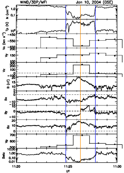
FIGURE 13. A zoom–in of the structure (bracketed by blue guidelines) in the far tail seen by Wind before the tail started to flap: A low-density, hot plasma is being ejected down the tail in a flux rope structure. The velocity moments are obtained from the PESA-HIGH instrument. See text for further details.

At the start and end of the interval (outside the time span bracketed by vertical blue guidelines), Wind is in the magnetosheath: hot and dense plasma moving antisunward at ∼540 km/s. Starting at around 11:25 UT Wind enters a large blob of lobe (low-ß) plasma in a flux rope-type structure which was being ejected at higher speeds (∼680 km/s) down the tail. The low density and high temperature are obtained from the PESA High spectrograms. The flux rope configuration is inferred from the enhanced B, peaking at the center, and the coherent rotations in the other field components. Taking the duration (2.9 min) and multiplying it by the plasma velocity (678 km/s) yields a scale size of the plasmoid of 18.4 R_E. Minimum variance analysis [53] gives an orientation for the flux rope axis of (−0.19, −0.24, 0.95) GSE, i.e., pointing strongly North. This would be a strange orientation in the tail if there were no twisting. (See discussion below where the effect of interplanetary By < 0 is taken into account.)

The magnetosheath flow has a significant positive Vy component (∼150 km/s), implying that the tail is deflected towards dusk. The tail axis makes an angle with the Sun-Earth line of ∼17°. This is evidence of the windsock effect, which results from the positive East-West flow component, Vy, seen by ACE at the CS (Figure 2; [40,42,54]).

How are the fast tailward-moving plasmoid at Wind and the fast sunward-moving twin-vortex pattern at F16 related? We suggest the following interpretation. The Wind and F16 observations point to the formation of an X line in the near-Earth tail region earthward of Wind. Wind observes the large plasmoid while F16 observes a fast sunward-flowing, rather large bursty bulk flow (BBF)-like structure (width of about 1 h in MLT).

The velocity shear between the BBF-like structure and the ambient plasma may lead to a vortex-like flow and a pair of upward-downward FACs ([55], their Figure 19) as they sweep aside the field lines, similar to Kelvin-Helmholtz vortices forming at the magnetopause boundary due to velocity shear [56,57]. However, the pair of FACs seen by F16 is in reverse order (the upward FAC is Westward rather than Eastward of the downward FAC), which may be attributed to the twisting of the tail produced by the torque exerted by IMF By.

Wind observes a tailward-flowing plasmoid at the distant tail in the lobe on open field lines. DMSP F16 observes fast vortex-like structures flowing sunward, just Earthward of the open-closed boundary (reconnection line; see Figure 11, fourth panel). Moreover, the F16 satellite also observes an upward and downward FAC near the open-closed field line boundary (Figure 12A, top panel), which would be consistent with the fast flow. In the upward FAC region, at −73.6° to −70.6° MLAT, F16 observes mono-energetic electrons, which is suggestive of the presence of a quasi-static upward electric field that accelerates the electrons downward and retards ion precipitation. This may partly explain the low ion energy fluxes in the F16 spectrogram. However, in the downward FAC region in Figure 12A from MLAT = −70.6° to −67.0°, the F16 ion energy fluxes remain low despite there being no evidence of mono-energetic electrons and, hence, of a significant upward electric field. The low ion and electron fluxes observed by F16 are quite noticeable when compared to those in the pre-midnight oval near the open-closed boundary observed by F13 (Figure 12B). F13 observes an upward FAC and there is some evidence of monoenergetic and broadband electrons, which can limit some ion precipitation. Yet, in spite of this, the ion energy fluxes in F13 observations are still higher than those in the downward FAC region in the F16 observations. The F16 electron energy fluxes also appear to be lower than their counterpart in the F13 observations.

Low ion and electron energy fluxes would be consistent with the scenario where the fast flow structure has depleted pressure and flux tube entropy (e.g., [58,59]). In Figure 12A, equatorward of the downward FAC region, the F16 ion and electron energy fluxes appear typical and are comparable to their counterpart in the F13 observations (Figure 12B). This would be expected because this region is not part of the fast flow region.

Additionally, we perform a very crude calculation of the timing when Wind and DMSP observe the disturbance. Wind, located ∼227 Re downtail, observes the plasmoid around 11:25–11:28 UT. The plasmoid moving at –621 km/s from the X-line around X ∼ −25 Re would reach Wind in about 34 min, assuming a constant plasmoid speed from the X-line to the Wind location. DMSP observes the fast flow structure around 11:00 UT. Assuming fast flow speed of 300 km/s, the timing would suggest an X-line forming in the ballpark of 10:51–10:54 UT

Summary and discussion

In this work, we analyzed an interlinked chain of effects in the M-I system elicited by a short (∼1/2 h) interplanetary non-reconnecting, bifurcated current sheet. The interplanetary structure was observed by ACE, ∼237 R_E upstream of Earth. Its signatures included a discontinuity in the gradients of the B and V profiles and concomitant Np-rise and B-dip near peak magnetic field strength. This structure was observed inside an ICME and its magnetic field was dominated by the East-West component, By, while strong non-radial flows (Vy and Vz) were reversing their polarity.

The magnetospheric response included: 1) in-out motions of the magnetopause and bow shock, 2) a local deformation of the magnetopause in the postnoon sector; 3) a 3 km/s sunward flow of a twin vortex pattern at the edge of the auroral oval, which was flanked by two sets of FACs, and associated with low ion and electron energy flux/pressure/flux tube entropy, having a large spatial scale (within 1 h in MLT), and 4) in the distant (∼−230 R_E) tail, a fast (∼−680 km/s) and large ejection of lobe-like plasma in a magnetic flux rope structure, which preceded observations of tail flapping. Using a reliable timer assured us that these phenomena are inter-related. The circumstances in which the IP feature occurs, in particular a strongly kinked, negative By (∼−15 nT) and a flow component Vy which had just transitioned from negative to positive, strongly twisted and deflected the tail from the Sun-Earth direction. It was possible to monitor the effects over such a long distance because of a good arrangement of spacecraft in the unperturbed solar wind, near the magnetopause, just below the magnetopause, and in the distant tail. The work thus illustrates how observations from an array of spacecraft spread throughout the magnetosphere can provide insight into, and whet our appetite for, magnetospheric dynamics.

Regarding the persistence of the density pulse, it is likely a structural feature of the current sheet related to its total internal pressure balance. The density change is not sharp like at a tangential discontinuity (TD) and does not induce new waves.

Interestingly, the event took place in otherwise very quiet geomagnetic conditions. As shown in Figure 14 (last 2 panels) the AE index was ∼0 nT and Sym-H ∼ −10 nT. The kink structure was embedded in a 5-to-6-h period (9-∼15 UT), starting in the recovery phase of a substorm and a (weak) storm, and finishing at the start of the growth phase of another substorm and an intensification of the ring current. As seen in the top panels (IP data are time-shifted to the magnetopause), this covered a period in the ICME around a maximum in B, positive Bz and a bipolar variation in By.

FIGURE 14

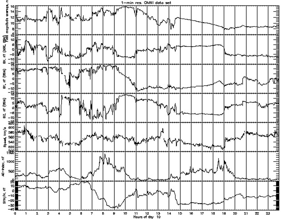
FIGURE 14. Data from the NASA OMNI website showing features of the interplanetary field and flow, and, in the bottom two panels, the substorm auroral electojet (AE) index and the storm-time Sym-H index. Interplanetary data are delayed to the magnetopause. At 11 UT, the time of arrival of the CS structure, both geomagnetic indices indicate very quiet conditions. Substorms appear a few hours before and after 11 UT.

With the strong interplanetary By (∼−15 nT), one would expect the geomagnetic tail to twist. We would expect the tail neutral sheet (NS) to be strongly twisted so that its normal would point towards–Y (GSE, West). Can this effect be seen in the in situ data at Wind? There are at least two indications. 1) Above, we derived the axis orientation of the flux rope at Wind, and found it to be mainly in the + z GSE direction. With the imposed twist this would be mainly along the Y-direction, which is an orientation more in line with what one would expect; 2) A further confirmation of the tail twist comes from the FAC polarities seen at F16 (Figure 12A). If we accept the hypothesis of a BBF-like origin, then the FAC polarity is in reverse order. From (55, their schematic Figure 19), the inward FAC (i.e., into ionosphere) is more towards dawn than the outward FAC. Here, however, the inward FAC occurs at 21 MLT and the outward at 22 MLT, i.e., the inward one is more toward the dusk than the outward one. However, a large enough twist would invert the location of the FACs in the dawn-dusk direction and restore agreement.

The IP medium had also a significant Vy component, which had turned positive shortly before our event (see Figures 2, 3). Interplanetary Vy is at the origin of the tail windsock effect [40,42,54], i.e., a deflection of the aberrated geomagnetic tail to align its axis along the solar wind flow. In our case the tail would be dragged toward dusk (i.e., tilted toward the + Y direction, where Wind was). This was also observed.

The North-South interplanetary component of the flow Vz varies over a significant range. Directional changes in this component have been argued to be the cause of the flapping of the tail [60–62]. Flapping consists of an up-down perturbation of the tail neutral sheet, advancing in the East-West direction and approaching the flanks [63]. From this we conclude that Vz is the major source of the tail flapping seen by Wind after the “precursor.”

We identified a nice “timer”, i.e., a rise in Np and a simultaneous drop in B, as an imprint of this event. Did we see this imprint in the Wind spacecraft observations? Taking a longer interval, we obtain a second peak in Np simultaneous with a minimum in B (Supplementary Figure S2, red traces) at 11:49 UT, i.e., 99 min after they were seen at ACE. From [64] we get an estimate of this delay if we divide the ACE-Wind separation by the solar wind speed (540 km/s). This estimate gives 92 min, which is in reasonable agreement. The CS lags behind the arrival of precursor (∼11:25 UT) by ∼24 min. This delay is expected since, as argued above, the CS triggers reconnection and the accelerated flows produced there travel inside the tail and outrun the SC, which travels in the solar wind [65].

Though multi-faceted, the effects in the M-I system do not indicate a system-wide response. Consider the F13 and F15 observations. F15 (Supplementary Figure S1 in the Supplementary Material S1), for example, observes the dusk auroral oval (not nightside) and observes signatures of Kelvin-Helmholtz instability near the open-closed boundary, which would be consistent with the high solar wind speed (∼540 km/s) observed during this event [56,57].

To conclude, in this paper we have focused on a clear interplanetary magnetic field and plasma structure. This feature consisted of a simultaneous drop in B and a rise in N which were accompanied by strong magnetic field and plasma flow changes. It was embedded in a—much larger—ICME, so that it would hardly have drawn any attention by itself had not a fortuitous deployment of spacecraft allowed us to monitor the multi-faceted response it elicited in the magnetosphere-ionosphere-magnetotail system over a radial distance of more than 400 Re.

Data availability statement

The original contributions presented in the study are included in the article/Supplementary Material, further inquiries can be directed to the corresponding author.

Author contributions

CF, SF, LW, DS, and SC, Develop idea, write manuscript and analyze data NL, RT, and JB: Contribute to interpretation.

Funding

CJF would like to acknowledge support from NASA Grants 80NSSC20K0197 and 80NSSC19K1293. SW acknowledges support of NASA grants 80NSSC20K0704, 80NSSC20K0188, 80NSSC22K0515, 80NSSC19K0843, 80NSSC21K1678. BJV is supported by the NASA Solar and Heliospheric Physics grant 80NSSC19K0832.

Acknowledgments

We are grateful to F. T. Gratton and N. V. Erkaev for helpful discussions.

Conflict of interest

The authors declare that the research was conducted in the absence of any commercial or financial relationships that could be construed as a potential conflict of interest.

Publisher’s note

All claims expressed in this article are solely those of the authors and do not necessarily represent those of their affiliated organizations, or those of the publisher, the editors and the reviewers. Any product that may be evaluated in this article, or claim that may be made by its manufacturer, is not guaranteed or endorsed by the publisher.

Supplementary material

The Supplementary Material for this article can be found online at: https://www.frontiersin.org/articles/10.3389/fphy.2022.942486/full#supplementary-material

References

1. Burlaga L., Sittler E., Mariani F., Schwenn R. Magnetic loop behind an interplanetary shock: Voyager, Helios, and IMP 8 observations. J Geophys Res (1981) 86:6673. doi:10.1029/ja086ia08p06673

CrossRef Full Text | Google Scholar

2. Gonzalez W. D., Tsurutani B. T. Criteria of interplanetary parameters causing intense magnetic storms (Dst<− 100 nT). Planey Space Sce (1987) 35(9):1101–9. doi:10.1016/0032-0633(87)90015-8

CrossRef Full Text | Google Scholar

3. Farrugia C. J., Burlaga L. F., Lepping R. P. Magnetic clouds and the quiet/storm effect at Earth: A review, in magnetic storms. In: T. B. Tsurutani, W. D. Gonzalez, Y. Kamide, and J. K. Arballo, editors. Geophysical monogr. Ser, vol. 98. Washington, D. C.: AGU (1997). p. 91.

CrossRef Full Text | Google Scholar

4. Farrugia C. J., Freeman M. P., Burlaga L. F., Lepping R. P., Takahashi K. The Earth's magnetosphere under continued forcing: Substorm activity during the passage of an interplanetary magnetic cloud. J Geophys Res (1993) 98:7657–71. doi:10.1029/92ja02351

CrossRef Full Text | Google Scholar

5. Huang C.-S., Reeves G. D., Borovsky J. E., Skoug R. M., Pu Z. Y., Le G. Periodic magnetospheric substorms and their relationship with solar wind variations. J Geophys Res (2003) 100:1255. doi:10.1029/2002JA009704

CrossRef Full Text | Google Scholar

6. Henderson M. G., Skoug R., Donovan E., Thomsen M. F., Reeves G. D., Denton M. H., et al. Substorms during the 10-11 August 2000 sawtooth event. J Geophys Res (2006) 111:A06206. doi:10.1029/2005JA011366

CrossRef Full Text | Google Scholar

7. Neugebauer M., Clay D. R., Goldstein B. E., Tsurutani B. T., Zwickl R. D. A reexamination of rotational and tangential discontinuities in the solar wind. J Geophys Res (1984) 89:5395. doi:10.1029/ja089ia07p05395

CrossRef Full Text | Google Scholar

8. Neugebauer M. The structure of rotational discontinuities. Geophys Res Lett (1989) 16(11):1261–4. doi:10.1029/gl016i011p01261

CrossRef Full Text | Google Scholar

9. Neugebauer M. Comment on the abundances of rotational and tangential discontinuities in the solar wind. J Geophys Res (2006) 111:A04103. doi:10.1029/2005JA011497

CrossRef Full Text | Google Scholar

10. Liu Y. D., Luhmann J. G., Kajdiz P., Kilpua E. K. J., Lugaz N., Nitta N. V., et al. Observations of an extreme storm in interplanetary space caused by successive coronal mass ejections. Nat Commun (2014) 5:3481. doi:10.1038/ncomms4481

PubMed Abstract | CrossRef Full Text | Google Scholar

11. Lugaz N., Farrugia C. J., Huang C.-L., Spence H. E. Extreme geomagnetic disturbances due to shocks within CMEs. Geophys Res Lett (2015) 42:4694–701. doi:10.1002/2015gl064530

CrossRef Full Text | Google Scholar

12. Farrugia C. J., Gratton F. T., Lund E. J., Sandholt P. E., Cowley S. W. H., Torbert R. B., et al. Two-stage oscillatory response of the magnetopause to a tangential discontinuity/vortex sheet followed by northward IMF: Cluster observations. J Geophys Res (2008) 113:A03208. doi:10.1029/2007JA012800

CrossRef Full Text | Google Scholar

13. Völk H. J., Auer R. D. Motions of the bow shock induced by interplanetary disturbances. J Geophys Res (1974) 79:40–8. doi:10.1029/ja079i001p00040

CrossRef Full Text | Google Scholar

14. Wu B. H., Mandt M. E., Lee L. C., Chao J. K. Magnetospheric response to solar wind dynamic pressure variations: Interaction of interplanetary tangential discontinuities with the bow shock. l Geophyl Re: Space Phys (1993) 98:21297. doi:10.1029/93JA01013

CrossRef Full Text | Google Scholar

15. Kaufmann R. L., Konradi A. Explorer 12 magnetopause observations: Large-scale nonuniform motion. J Geophys Res (1969) 74:3609–27. doi:10.1029/ja074i014p03609

CrossRef Full Text | Google Scholar

16. Sibeck D. G. A model for the transient magnetospheric response to sudden solar wind dynamic pressure variations. J Geophys Res (1990) 95:3755. doi:10.1029/ja095ia04p03755

CrossRef Full Text | Google Scholar

17. Fairfield D. H., Farrugia C. J., Mukai T., Nagai T., Fedorov A. Motion of the dusk flank boundary layer caused by solar wind pressure changes and the kelvin-helmholtz instability: 10–11 january 1997. Geophy. Re. (2003) 108:A121460. doi:10.1029/2003JA010134

CrossRef Full Text | Google Scholar

18. Maynard N. C., Farrugia C. J., Ober D. M., Burke W. J., Dunlop M., Mozer F. S., et al. Cluster observations of fast shocks in the magnetosheath launched as a tangential discontinuity with a pressure increase crossed the bow shock. J Geophys Res (2008) 113:A10212. doi:10.1029/2008JA013121

CrossRef Full Text | Google Scholar

19. Thomsen M. F., Thomas V. A., Winske D., Gosling J. T., Farris M. H., Russell C. T., et al. Observational test of hot flow anomaly formation by the interaction of a magnetic discontinuity with the bow shock. J Geophys Res (1993) 98:15319. doi:10.1029/93ja00792

CrossRef Full Text | Google Scholar

20. Sibeck D. G., Borodkova N. L., Schwartz S. J., Owen C. J., Kessel R. Comprehensive study of the magnetospheric response to a hot flow anomaly. J Geophys Res (1999) 104(A3):4577–93. doi:10.1029/1998ja900021

CrossRef Full Text | Google Scholar

21. Schwartz S. J., Paschmann G., Sckopke N., Bauer T. M., Dunlop M., Fazakerly A. N., et al. Geophy. Re. (2000) 105(12):639650–12.

22. Smith C. W., L'heureux J., Ness N. F., Acuna M. H., Burlaga L. F., Scheifele J. The ACE magnetic fields experiment. Space Sc. Re. (1998) 86:613–32.

CrossRef Full Text | Google Scholar

23. McComas D. J., Bame S. J., Barker P., Feldman W., Phillips J., Riley P., et al. Solar wind electron proton alpha monitor (SWEPAM) for the advanced composition explorer. Space Sc. Re. (1998) 86:563–612. doi:10.1023/A:1005040232597

CrossRef Full Text | Google Scholar

24. Lepping R. P., Acuna MH, Burlaga LF, Farrell WM, Slavin JA, Schatten KH, et al. The wind magnetic field investigation. Space Sci Rev (1995) 71:207–29. doi:10.1007/bf00751330

CrossRef Full Text | Google Scholar

25. Lin R. P., Anderson KA, Ashford S, Carlson C, Curtis D, Ergun R, et al. A three-dimensional plasma and energetic particle investigation for the wind spacecraft. Space Sci Rev (1995) 71:125–53. doi:10.1007/bf00751328

CrossRef Full Text | Google Scholar

26. Wilson L. B., Brosius A. L., Gopalswamy N., Nieves-Chinchilla T., Szabo A., Hurley K., et al. A quarter century of Wind spacecraft discoveries. Res Geophys (2021) 59:e2020RG000714. doi:10.1029/2020RG000714

CrossRef Full Text | Google Scholar

27. Kokubun S., Yamamoto T., Acuna M. H., Hayashi K., Shiokawa K., Kawano H. The geotail magnetic field experiment . Geoma. Geoelect. (1994) 46:7–21. doi:10.5636/jgg.46.7

CrossRef Full Text | Google Scholar

28. Mukai T., Machida S., Saito Y., Hirahara M., Terasawa T., Kaya N., et al. The low energy particle (LEP) experlment onboard the GEOTAIL satellite. JGgeomagnGgeoelec (1994) 46:669–92. doi:10.5636/jgg.46.669

CrossRef Full Text | Google Scholar

29. Balogh A., Carr CM, Acuna MH, Dunlop MW, Beek TJ, Brown P, et al. The Cluster magnetic field investigation: Overview of inflight performance and initial results. Ann Geophys (2001) 19:1207–17. doi:10.5194/angeo-19-1207-2001

CrossRef Full Text | Google Scholar

30. Rème H., Aoustin C, Bosqued JM, Dandouras I, Lavraud B, Sauvaud JA, et al. First multispacecraft ion measurements in and near the Earth’s magnetosphere with the identical Cluster ion spectrometry (CIS) experiment. Ann Geophys (2001) 19:1303–54. doi:10.5194/angeo-19-1303-2001

CrossRef Full Text | Google Scholar

31. Russell C. T., Snare R. C., Means J. D., Pierce D, Dearborn D, Larson M, et al. The GGS/POLAR magnetic fields investigation. Space Sci Rev (1995) 71:563–82. doi:10.1007/BF00751341

CrossRef Full Text | Google Scholar

32. Scudder J., Hunsacker F., Miller G., Lobell J, Zawistowski T, Ogilvie K, et al. Hydra — a 3-dimensional electron and ion hot plasma instrument for the polar spacecraft of the ggs mission. Space Sci Rev (1995) 71:459–95. doi:10.1007/bf00751338

CrossRef Full Text | Google Scholar

33. Hardy D. A., Schmitt L. K., Gussenhoven M. S., Marshall F. J., Yeh H. C, Shumaker T. L., et al. Precipitating electron and ion detectors (SSJ/4) for the block 5D/flights 6-10 DMSP satellites: Calibration and data presentation, rep. AFGL-TR-84-0317, air force geophys. Mass: Lab., Hanscom Air Force Base (1984).

34. Rich F. J., Hardy D. A., Gussenhoven M. S. Enhanced ionosphere-magnetosphere data from the DMSP satellites. Eos Trans AGU (1985) 66:513. doi:10.1029/eo066i026p00513

CrossRef Full Text | Google Scholar

35. Wing S., Johnson J. R. Theory and observations of upward field-aligned currents at the magnetopause boundary layer. Geophys Res Lett (2015) 42:9149–55. doi:10.1002/2015GL065464

PubMed Abstract | CrossRef Full Text | Google Scholar

36. Johnson J. R., Wing S. The dependence of the strength and thickness of field-aligned currents on solar wind and ionospheric parameters. J Geophys Res Space Phys (2015) 120:3987–4008. doi:10.1002/2014JA020312

PubMed Abstract | CrossRef Full Text | Google Scholar

37. Wing S., Ohtani S. I., Newell P. T., Higuchi T., Ueno G., Weygand J. M., et al. Dayside field-aligned current source regions. J Geophys Res (2010) 115:A12215. doi:10.1029/2010JA015837

CrossRef Full Text | Google Scholar

38. Richardson I.G., Cane H.V. Near-earth interplanetary coronal mass ejections during solar cycle 23 (1996 – 2009): Catalog and summary of properties. Sol Phys (2010) 264:189–237. doi:10.1007/s11207-010-9568-6

CrossRef Full Text | Google Scholar

39. Al-Haddad N., Galvin A. B., Lugaz N., Farrugia C. J., Yu W. Investigating the cross-section of coronal mass ejections through the study of non-radial flows with STEREO/PLASTIC.Astrophysical J (2021) 927(1):68.

Google Scholar

40. Shodhan S., Siscoe G. L., Frank L. A., Ackerson K. L., Paterson W. R. Boundary oscillations at Geotail: Windsock, breathing, and wrenching. J Geophys Res (1996) 101(A2):2577–86. doi:10.1029/95ja03379

CrossRef Full Text | Google Scholar

41. Shang W. S., Tang B. B., Shi Q. Q., Tian A. M., Zhou X. Y., Yao Z. H., et al. Unusual location of the geotail magnetopause near lunar orbit: A case study. J Geophys Res Space Phys (2019) 125(4):e2019JA027401. doi:10.1029/2019ja027401

CrossRef Full Text | Google Scholar

42. Borovsky J. E. The effect of sudden wind shear on the Earth's magnetosphere: Statistics of wind shear events and CCMC simulations of magnetotail disconnections. J Geophys Res (2012) 117(A6). doi:10.1029/2012ja017623

CrossRef Full Text | Google Scholar

43. Borovsky J.E. Looking for evidence of wind-shear disconnections of the earth's magnetotail: GEOTAIL measurements and LFM MHD simulations. J Geophys Res Space Phys (2018) 123(7):5538–60. doi:10.1029/2018ja025456

CrossRef Full Text | Google Scholar

44. Cowley S. W. H. Magnetospheric asymmetries associated with the Y-component of the IMF. Planet Space Sci (1981) 29:79–96. doi:10.1016/0032-0633(81)90141-0

CrossRef Full Text | Google Scholar

45. Wing S., Newell P. T., Sibeck D. G., Baker K. B. A large statistical study of the entry of interplanetary magnetic field Y-component into the magnetosphere. Geophys Res Lett (1995) 22:2083–6. doi:10.1029/95GL02261

CrossRef Full Text | Google Scholar

46. Russell C. T., Melliot M. M., Smith E. J., King J. H. Multiple spacecraft observations of interplanetary shocks: Four spacecraft determinations of shock normals. . Geophy. Re. (1983) 88:4739–5408.

CrossRef Full Text | Google Scholar

47. Knetter T., Neubauer F. M., Horbury T., Balogh A. Four-point discontinuity observations cluster magnetic field data: A statistical survey. JGgeomagnGgeoelec (2004) 109:A06102. doi:10.5636/jgg.46.7

CrossRef Full Text | Google Scholar

48. Farrugia C. J., Cohen I. J., Vasquez B. J., Lugaz N., Alm L., Torbert R. B., et al. Effects in the near-magnetopause magnetosheath elicited by large-amplitude Alfvénic fluctuations terminating in a field and flow discontinuity. J Geophys Res Space Phys (2018) 123(11):8983–9004. doi:10.1029/2018ja025724

CrossRef Full Text | Google Scholar

49. Wing S., Gkioulidou M., Johnson J. R., Newell P. T., Wang C.-P. Auroral particle precipitation characterized by the substorm cycle. J Geophys Res Space Phys (2013) 118:1022–39. doi:10.1002/jgra.50160

CrossRef Full Text | Google Scholar

50. Newell P. T., Sotirelis T., Wing S. Diffuse, monoenergetic, and broadband aurora: The global precipitation budget. J Geophys Res (2009) 114:A09207. doi:10.1029/2009JA014326

CrossRef Full Text | Google Scholar

51. Wing S., Newell P. T. Central plasma sheet ion properties as inferred from ionospheric observations. J Geophys Res (1998) 103(A4):6785–800. doi:10.1029/97JA02994

CrossRef Full Text | Google Scholar

52. Wing S., Newell P. T. 2D plasma sheet ion density and temperature profiles for northward and southward IMF. Geophys Res Lett (2002) 29(9):21. doi:10.1029/2001GL013950

CrossRef Full Text | Google Scholar

53. Sönnerup B. U. Ö., Scheible M. Minimum andmaximum variance analysis. In: G. Paschmann, and P. W. Daly, editors. Analysis methods for multi-spacecraft data. Bern, Switzerland: International Space Science Institute (1998). p. 185–220.

Google Scholar

54. Grygorov K., Přech L., Šafránková J., Němeček Z., Goncharov O. The far magnetotail response to an interplanetary shock arrival. Planey Space Sce (2014) 103:228–37. doi:10.1016/j.pss.2014.07.016

CrossRef Full Text | Google Scholar

55. Birn J., Raeder J., Wang Y. L., Wolf R. A., Hesse M., On the propagation of bubbles in the geomagnetic tail. Ann Geophys (2004) 22(5): 1773–86. Copernicus GmbH. doi:10.5194/angeo-22-1773-2004

CrossRef Full Text | Google Scholar

56. Johnson J. R., Wing S., Delamere P., Petrinec S., Kavosi S. Field-aligned currents in auroral vortices. J Geophys Res Space Phys (2021) 126:e2020JA028583. doi:10.1029/2020JA028583

CrossRef Full Text | Google Scholar

57. Petrinec S. M., Wing S., Johnson J. R., Zhang Y. Multi-spacecraft observations of fluctuations occurring along the dusk flank magnetopause, and testing the connection to an observed ionospheric bead. Front Astron Space Sci (2022) 9:827612. doi:10.3389/fspas.2022.827612

CrossRef Full Text | Google Scholar

58. Pontius D. H., Wolf R. A. Transient flux tubes in the terrestrial magnetosphere. Geophys Res Lett (1990) 17(1):49–52. doi:10.1029/gl017i001p00049

CrossRef Full Text | Google Scholar

59. Wing S., Johnson J. R., Chaston C. C., Echim M., Escoubet C. P., Lavraud B., et al. Review of solar wind entry into and transport within the plasma sheet. Space Sci Rev (2014) 184:33–86. doi:10.1007/s11214-014-0108-9

CrossRef Full Text | Google Scholar

60. Runov A., Angelopoulos V., Sergeev V. A., Glassmeier K. H., Auster U., McFadden J., et al. Global properties of magnetotail current sheet flapping: THEMIS perspectives. Ann Geophys (2009) 27:319–28. doi:10.5194/angeo-27-319-2009

CrossRef Full Text | Google Scholar

61. Sergeev V. A., Tsyganenko N. A., Angelopoulos V. Dynamical response of the magnetotail to changes of the solar wind direc-tion: An MHD modeling perspective. Ann Geophys (2008) 26:2395–402. doi:10.5194/angeo-26-2395-2008

CrossRef Full Text | Google Scholar

62. Farrugia C. J., Rogers A. J., Torbert R. B., Genestreti K. J., Nakamura T. K. M, Lavraud B., et al. An encounter with the ion and electron diffusion regions at a flapping and twisted tail current sheet. JGR Space Phys (2021) 126:e2020JA028903. doi:10.1029/2020JA028903

CrossRef Full Text | Google Scholar

63. Sergeev V. A., Runov A., Baumjohann M., Nakamura R., Zhang T. L., Volwerk M., et al. Current sheet flapping motion and structure observed by cluster. Geophys Res Lett (2003) 30:1327. doi:10.1029/2002GL016500

CrossRef Full Text | Google Scholar

64. Kaymaz Z., Petschek H. E., Siscoe G. L., Frank L. A., Ackerson K. L., Paterson W. R., et al. Disturbance propagation times to the far tail. J Geophys Res (1995) 100(A12):23743. doi:10.1029/95ja02855

CrossRef Full Text | Google Scholar

65. Sugiura M., Skillman T. L., Ledley B. G., Heppner J. P. Propagation of the sudden commencement of July 8, 1966, to the magnetotail. J Geophys Res (1968) 73(21):6699–709. doi:10.1029/ja073i021p06699

CrossRef Full Text | Google Scholar