Enabling Persistent Autonomy for Underwater Gliders with Ocean Model Predictions and Terrain-Based Navigation

1. Introduction

Aquatic robots, such as Autonomous Underwater Vehicles (AUVs), and their supporting infrastructure play a major role in the collection of oceanographic data (e.g., Godin et al. (2006), Paley et al. (2008), and Whitcomb et al. (1999)). Actively actuated (propeller-driven) underwater vehicles have proven effective in multiple sampling scenarios; however, they have limited deployment endurance. The emergence of buoyancy-driven vehicles, i.e., underwater gliders, has enabled greater energy savings and thus increased endurance. With limited actuation, these vehicles are more susceptible to external forces, e.g., ocean currents, resulting in poor navigational and localization accuracy underwater. This is exacerbated in coastal regions, where current velocities can be the same order of magnitude as the vehicle velocity. Autonomous underwater gliders provide an approach to observing ocean processes up close. These vehicles are capable of long-term deployments, remaining out in the ocean for periods of time ranging from several weeks to several months (Davis et al., 2008). Although their horizontal speeds are only about 1 km/h, their longevity, coupled with the use of multiple gliders, can be compensated by providing an extended temporal and spatial series of observations.

Our work is motivated by the desire to enable intelligent data collection of complex dynamics and processes that occur in a coastal ocean environments to further our understanding and prediction capabilities. Of particular interest is the formation and evolution of Harmful Algal Blooms (HABs) in the Southern California Bight (SCB), an oceanic region contained within 32° N to 34.5° N and −117° E to −121° E. This region is under continued study to uncover the connections between small-scale biophysical processes and large-scale events related to algal blooms, specifically blooms composed of toxin-producing species (i.e., HABs) (Jones et al., 2002; Schnetzer et al., 2007; Smith et al., 2010b). The long-term study utilizes a team of two autonomous gliders (He Ha Pe and Rusalka), owned and operated by the USC Center for Integrated Networked Aquatic PlatformS (CINAPS) team (Smith et al., 2010b), to sample off the coast of southern California. Field data examined within this paper were gathered during missions executed by these vehicles. The Jet Propulsion Laboratory, California Institute of Technology, maintains a high-resolution, large-scale regional ocean model for the SCB, and provided the model predictions used for our simulation comparisons (Vu, 2008).

Autonomous gliders can spend in excess of 8-h dead reckoning under water, navigating by only a compass, magnetometer, and depth sensor. Frequent surfacing for position fixes limits the amount of data that is collected during a deployment by decreasing the total time underwater, and by expending excess energy for communication and localization while on the surface. Moreover, surfacing in potentially hazardous locations (e.g., shipping lanes) puts the vehicle at risk. Maximizing time underwater significantly reduces the ability of the vehicle to localize. Additionally, accurately reconstructing subsurface glider trajectories can be difficult for long underwater transects; it is generally assumed that the traversed path of a glider is the straight line connecting the dive and surface locations, which is a poor assumption most of the time.

To assist with energy savings, most gliders do not employ highly accurate (high-energy) navigation systems but rely on dead reckoning with a modest Inertial Measurement Unit (IMU). Regardless of the specifications of the IMU, sensor drift is unbounded and navigational error increases with time. During routine deployments in a coastal ocean environment in Los Angeles, CA, USA, it was found that typical underwater gliders experience roughly 650 m navigational error for each kilometer traveled (Smith et al., 2010c, 2012). A combination of these factors can lead to poor experimental results. For example, Figure 1 displays a planned path in black, and an actual execution of this planned path by a glider in white. This poses difficulties in both plan execution in situ and reconstructing the actual traversed path of the vehicle for analysis of scientific data. Additionally, for operations in cluttered environments, or near shipping lanes, this error may put the vehicle at serious risk (Pereira et al., 2013). With an Unscented Kalman Filter (UKF) and inertial dead reckoning augmented with ocean model predictions, the authors have shown that this error can be reduced to less than 500 m over a single kilometer of travel (Smith et al., 2010c, 2012); this is still significant when trying to avoid a busy shipping lane or reconstructing a dataset. High-level planning can provide assurance that the vehicle will follow a prescribed trajectory (Pereira et al., 2013); however, we are always faced with potential navigation error during plan execution. In Smith et al. (2013), it is shown that an approach solely based on ocean model predictions breaks down in regions of significant bathymetric relief, where ocean models have poor prediction capabilities. However, these regions of significant bathymetric relief are exactly where a terrain-based navigation approach is able to perform well. Here, we examine the utility of integrating terrain-based navigation methods into an existing framework for improving the navigational accuracy of underwater gliders. Specifically, we propose to utilize ocean model predictions within a UKF to improve planning and navigation capabilities while additionally incorporating a terrain-based navigation method for localization during plan execution.

FIGURE 1

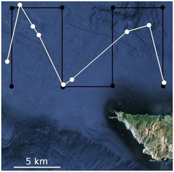
Figure 1. A planned lawnmower path (black) and actual executed path (white) for a glider deployment near the northern tip of Santa Catalina Island, CA, USA.

Areas of significant productivity in the coastal ocean are highly correlated with locations of significant bathymetric relief, e.g., algal blooms (Horner et al., 1997; Anderson et al., 2002; Fulton-Bennett, 2005; Kudela et al., 2005; Sekula-Wood et al., 2009) and ocean fronts (Mancho et al., 2008; Ferrari, 2011; Zhang et al., 2013). In these areas, every path traversed by an AUV has a depth signature that is highly variable and becomes increasingly unique the longer the trajectory becomes. These specific deployment locations and science motivations enhance the utility of terrain-based methods to increase navigation accuracy and localization for long-duration missions.

The use of prior information in the form of predictive ocean models has been shown to improve mission accuracy and execution during field trials (Smith et al., 2010c, 2012). While these models have become quite advanced, they are still generally discrete and deterministic in nature. Specifically, there is no metric provided on the confidence or covariance of the predicted variable, and accurate interpolations of the discrete measurements require sophisticated data-processing algorithms to augment the predictions. The developers of both ROMS and HOPS have investigated producing ensemble forecasts for their model. This method perturbs initial and/or boundary conditions to produce a set of forecasts. This ensemble forecast provides a distribution of potential outcomes; however, the sample size is often too small (~12) to provide a meaningful variance measure of the prediction. These ensembles can provide an accuracy estimation of the model output; however, this is more related to the sensitivity of the numerical model to the inputs rather than the actual physical variability of the ocean inherent within the domain of the model. The size of the ensemble forecast is limited only by computational power and time. However, as models provide the most accurate predictions in the times closest to the observations and measurements, we cannot spend an excessive amount of time computing all the possible ensemble outcomes. So, we are forced to compromise working to produce the most accurate models utilizing a minimal set of resources or utilizing additional resources to augment the computation of model reliability and variability. In current research, several assimilation techniques, e.g., Kalman filter-based ensemble forecasts (Rixen et al., 2009), and variational schemes, e.g., 4DVar (Powell et al., 2008), are under investigation in the modeling community, with the goal to get the model output closer to the observed values.

Predictive models have been exploited in previous AUV mission planning efforts, where a main focus has been to compute energy-optimal paths, as the majority of applications utilize propeller-driven, short-duration (<24 h) AUVs. The work in Garau et al. (2005) makes use of the A* search procedure to harness the inherent spatial variability of currents and minimize expended energy. Similarly, the authors in Alvarez et al. (2004) employ a genetic algorithm to generate energy-conserving trajectories for an AUV subject to time-varying currents. Research in Witt and Dunbabin (2008) explores the utility of predictive models to aid in avoiding land masses exposed by ebbing tides, while the investigation in Kruger et al. (2007) examines how predictions can be used to “ride” currents in estuarine and riverine environments. Although the methodologies, domains, and applications are different, the underlying models used are all deterministic, providing a fixed value for the current at a specified location and time. Much recent research in robotics leverages probabilistic planning and control methods, and has the potential to be applied to the marine domain [e.g., Ono and Williams (2008), Rao and Williams (2009), Hollinger et al. (2012)]. Hence, it is critical to understand the probabilistic nature and/or variability of the priors that will best enable ocean sampling, e.g., predictive ocean models.

However, even with good ocean models, underwater gliders still use dead reckoning while underway. As a proprioceptive device, an IMU is one navigation aid that can be utilized in underwater environments without requiring external electromagnetic signal reception. IMU error sources and their effects on navigation performance are discussed in Flenniken et al. (2005), which demonstrates that even using tactical-grade sensors, the inevitable drift is still too high to mitigate substantial trajectory errors. Navigation is not reliable using IMU data alone, especially when localization fixes are scarce, and sensor drift cannot be bounded.

A detailed survey of recent advances and current challenges in underwater navigation, summarizing existing work on Terrain-Based Navigation (TBN) for underwater vehicles, is provided in Kinsey et al. (2006). One clearly identified shortcoming of TBN in the aquatic environment is the lack of accurate, high-resolution maps of the sea floor in many regions. Additionally, sensor limitations, especially the limitations of optical range sensors, substantially restrict TBN underwater. In Kinsey et al. (2006), it is concluded that improved navigation will enable new missions that would previously have been considered infeasible or impractical. The idea of terrain-based navigation is not new; significant research was carried out on the use of TBN for long-range missile guidance prior to the development of the GPS satellite network (Golden, 1980). Here, we apply a similar concept to an underwater glider.

Recent work by Lagadec (2010) on TBN under ice has demonstrated the feasibility of using a particle filter for long-term glider navigation. Lower relief maps, with a resolution of 2 km, of regions above the arctic circle were sufficient to navigate with reasonable accuracy (~1 km accuracy, with a mean accuracy of approximately 8 km in one simulation). The study suggests that for real deployments, technological advances would be necessary to achieve the required navigation performance. However, higher relief bathymetric maps could facilitate the implementation of a TBN that operates online, in real time. The primary limitation of the technique presented in Lagadec (2010) was the lack of an accurate terrain map, which does not invalidate the methodology used. A significant difference between this method and the proposed is that the use of a particle filter relies both on an accurate terrain map and a dynamic model to propagate the state. Our proposed TBN method does not rely on an underlying dynamic model, although adding a dynamic vehicle model to our TBN approach will improve the presented results.

A number of other studies have utilized particle filters as part of a TBN framework for underwater vehicles (Gustafsson et al., 2002; Anonsen and Hallingstad, 2006, 2007; Lagadec, 2010). The particle filter is suitable as a solution to the TBN problem because it is probabilistic (and therefore captures environmental uncertainty), and because it naturally incorporates the property that the longer a path is traversed, the more likely a single solution will emerge. Again, filtering requires a known motion model for the vehicle, in order to weight possible trajectories according to the dynamics achievable by the system. A simple motion model has limitations when applied to underwater gliders, as a significant portion of the glider motion is driven by ocean currents that can be of the same order of magnitude as the nominal vehicle velocity. Hence, the accuracy of a glider motion model depends heavily on an ability to predict ocean currents, which can be difficult in highly dynamic environments such as the coastal ocean. The method proposed herein is developed as a model-free approach to the TBN problem, using only the acquired water depth data and the initial heading to the next prescribed waypoint. Although this approach is deterministic in nature, it does not rely on a vehicle or ocean model.

This paper examines the combination of two methods for improving both navigation and localization, not only for real-time state estimation but also for accurately reconstructing the actual path that the vehicle traversed to contextualize the gathered data. The overarching goal is to provide an online method for autonomous gliders to accurately navigate in coastal regions. We combine a predictive approach that incorporates glider motion derived from an IMU and ocean model predictions into an UKF with a real-time, terrain-based navigation (TBN) algorithm. The UKF algorithm provides mission planning and a navigation strategy, while the TBN algorithm provides accurate localization during mission execution. The UKF integrates data from an IMU, and the TBN algorithm utilizes only the depth, altitude, and initial compass heading from start to goal; thus, the entire system operates model-free. Practically, TBN for underwater vehicles is limited by the altitude sensor’s ability to see the ground, which is not a limiting factor for most coastal and shallow (<200 m) operations.

The presented approach builds upon prior work by the authors in both the incorporation of ocean models for planning and the use of terrain-based navigation for real-time localization and path reconstruction (Stuntz et al., 2015). The primary contributions of this paper combine these approaches into a single, implementable algorithm, as well as extend existing results in the following four ways.

1. We apply our TBN algorithm to multiple glider missions with varying trajectory length, mission time, and bathymetric relief, further demonstrating the utility of the proposed method.

2. The additional results from extended applications of the TBN algorithm demonstrate the capability of the proposed method to accurately reconstruct the actual paths that gliders followed during mission execution.

3. We present an algorithm that combines the predictive ocean model-based UKF method with the TBN algorithm to provide a robust methodology for maintaining a fixed navigational uncertainty for underwater gliders.

4. We demonstrate that the combination of our two methods into a single algorithm can (a) be run in real time, on-board an underwater glider and (b) maintains a prescribed navigational error for all executed missions.

The proposed methodologies have been tested with data from multiple deployments of Slocum autonomous gliders off the coast of California, USA. Results are presented that demonstrate a significant increase in navigational accuracy compared with previously reported results.

2. Background

2.1. Autonomous Underwater Gliders

The vehicle for this study is a Webb Slocum autonomous underwater glider (Webb Research Corporation, 2008) as seen in Figure 2. A Slocum glider is a 1.5-m (length) by 21.3 cm (diameter), torpedo-shaped vehicle designed for long-term (~1 month) ocean sampling and monitoring (Griffiths et al., 2007; Schofield et al., 2007). These vehicles fly through the water driven entirely by a variable buoyancy system. Wings convert the buoyancy-dependent vertical motion into forward velocity. Inflection points occur at depths and altitudes set in the user-defined mission plan. Thus, the glider navigates by dead reckoning between waypoints with a sequence of dives and climbs (yo-yos), forming a vertical sawtooth pattern.

FIGURE 2

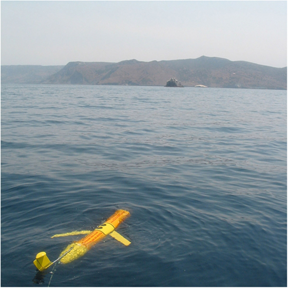
Figure 2. A CINAPS (Smith et al., 2010b) Slocum glider preparing to start a mission off the Northeast coast of Santa Catalina Island, CA, USA.

Gliders are utilized for their deployment endurance, as they provide an optimal method for generating high-resolution spatial and temporal data with minimal energy expense. Sophisticated and power-hungry navigational instruments are not common due to the reduction in deployment duration resulting from their increased power consumption. For similar reasons, on-board decision making and computation are generally not performed. A Slocum glider includes a GPS receiver for localization at each surfacing. In addition to the GPS receiver, a typical glider carries a PNI TCM2 attitude sensor and a SBE 41CP pressure sensor on-board. The TCM2 incorporates an electronic compass, a three-axis magnetometer, and a two-axis tilt sensor, and it is able to provide attitude data at a user-selectable rate of 1–30 Hz, heading accuracy of ±1° RMS, and roll/pitch accuracy of approximately ±0.2° RMS. The SBE measures pressure with an RMS accuracy of 2 dbar or depth with an RMS accuracy of 2.03 m near the water surface, at a rate of 1 Hz. In addition, each glider incorporates a Sea Bird non-pumped, low drag conductivity, temperature, and depth package. A 500-psi pressure transducer is used for the depth measurement. An Airmar altimeter, 0–100 m range transducer, and electronics are supported on the Displacement Piston Pump Cylinder. The transducer is mounted such that it is parallel to a flat sea bottom at a dive angle of nominally 26°.

2.2. Dead-Reckoning Error Estimation

Based on the results of initial tests presented in Smith et al. (2010b), we are motivated to further investigate the improvement of navigational capabilities of gliders by use of TBN. Since a glider depends solely upon dead reckoning for subsurface navigation, the uncertainty in the estimated state will grow without bound. For our applications in the coastal regions of Southern California, we generally require the vehicle to surface frequently (every 3–6 h), see, e.g., Smith et al. (2010a,b, 2011a). Since we acquire GPS ground truth relatively frequently, we are able to bound the growth of the state estimation error. This provides a baseline expected error for the assessment of navigational accuracy and precision. In this paper, we are interested in better localization, while underwater between waypoints to enable more accurate reconstructions of executed trajectories.

During a deployment, a Slocum glider navigates by the following method: when navigating to a new waypoint, the present location L of the vehicle is compared to the next prescribed waypoint in the mission file (W_i), and a bearing and range are computed for execution of the next segment of the mission. The geographical location at the extent of the computed bearing and range from L is the aiming point A_i. The vehicle dead-reckons with the computed bearing and range toward A_i, with the intent of surfacing at W_i. The computed bearing is not altered, and the glider must surface to make any corrections or modifications to its dive plan. When the glider determines that it has traveled the requested range at the specified bearing (based on speed over ground estimation from the previous dive), it surfaces and acquires a GPS fix. If the vehicle surfaces within a given range of W_i, the waypoint is determined to be achieved. Positional error between the actual surfacing location and W_i is computed, and is fully attributed to environmental disturbances, i.e., ocean currents. A depth-averaged current vector is computed, and this is factored in when computing the range and bearing to W_i+1. Hence, A_i is in general not in the same physical location as W_i and rarely does the glider ever surface at W_i. It is of interest to note that A_i is computed from the error observed in the previously executed leg and does not make a prediction or take into account the fact that the vehicle may not be moving through a similar current regime.

2.3. Terrain-Based Navigation

Prior to satellite-based navigation, e.g., GPS, long-distance navigation systems were developed for missiles (Golden, 1980). Data from an embedded altimeter were compared to ground elevations that were provided in a stored map or look-up table. The navigational accuracy of this method is dependent upon the resolution of the underlying topography map and the accuracy of the elevation measurement; both very good for terrestrial applications. This system became redundant after the introduction of GPS, although it is still a useful navigational aid for GPS-denied environments, e.g., underwater. Until recently, the utility of terrain-based navigation for underwater vehicles was low due to the poor resolution of bathymetric maps. Updated bathymetry maps with higher resolution provide motivation for revisiting the application of this method for low-power, accurate navigation underwater. Here, we utilize publicly available maps provided by the Southern California Coastal Ocean Observing System (SCCOOS) which provide 30 arc second grid resolution (SCCOOS, 2009). A detailed representation of the SCCOOS bathymetry map for the southern California region of interest is presented in Figure 3. Additionally, given the increase in accuracy of low-cost sensors for dead reckoning, e.g., IMUs, and increased skill of ocean models, it is of interest to investigate a combined approach to increasing underwater navigation.

FIGURE 3

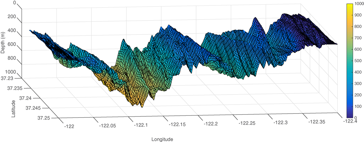
Figure 3. Bathymetry data mapped and shaded, showing detail of the SCCOOS data in Monterey Bay. Maps are accurate to 0.0008° in both latitude and longitude.

3. Unscented Kalman Filter and Ocean Model Prediction Algorithm

Through previous research efforts, we have developed a simulation tool for glider missions in the SCB that incorporates the ROMS predictions of the 3D velocity field (Smith et al., 2010c, 2012). We fuse the measurements from the sensors (either actual in real-time or simulated post priori) into an Unscented Kalman Filter (UKF) to estimate the position, attitude, and velocity of the vehicle over time (Julier and Uhlmann, 2004).

The UKF is a Bayesian filtering algorithm which employs a statistical local linearization procedure to propagate and update the system state. For non-linear systems, this approach typically produces significantly more accurate estimates than the analytic local linearization employed by the well-known Extended Kalman filter (EKF) (Huster and Rock, 2003). In our case, the 10 × 1 state vector is

$\mathbf{x}(t)={{\displaystyle \left[{{\displaystyle \left({\mathbf{p}}^W(t)\right)}}^T{{\displaystyle \left({{\displaystyle \overline{q}}}_B^W(t)\right)}}^T{{\displaystyle \left({\mathbf{v}}^B(t)\right)}}^T\right]}}^T,$ (1)

where p^W(t) is the position of the glider in the world (UTM) frame, ${{\displaystyle \overline{q}}}_B^W(t)$ is the unit quaternion that defines the attitude of the glider body relative to the world frame, and v ^B(t) is the velocity of the glider in the body frame. This simple kinematic model is sufficient for this application of long-range planning. A primary motivation for our choice of the UKF is its performance with a more sophisticated (and non-linear) dynamic model of the glider, which we are exploring in a parallel effort.

For our simulation, we assume that the glider follows a nominal, linear sawtooth trajectory, and that the vehicle angular rotation rate and linear acceleration are driven by white, zero-mean Gaussian noise processes represented by the vectors η_q(t) and η_v(t), with covariance matrices Q_q and Q_v, respectively. The system state evolves in continuous time according to

${{\displaystyle \dot{p}}}^W\text{}(t)=C\left({{\displaystyle \overline{q}}}_B^W(t)\right)v^B(t),$ (2)

${{\displaystyle \dot{\overline{q}}}}_B^W(t)=\frac{1}{2}\Omega \left({\eta }_q(t)\right){{\displaystyle \overline{q}}}_B^W(t),$ (3)

${{\displaystyle \dot{v}}}^B(t)={\eta }_v(t),$ (4)

where $C\left({{\displaystyle \overline{q}}}_B^W(t)\right)$ is the direction cosine matrix corresponding to the unit quaternion ${{\displaystyle \overline{q}}}_B^W(t)$, and Ω(η_q(t)) is the quaternion kinematic matrix, relating the rate of change of the orientation quaternion to the body frame angular velocity (Stevens and Lewis, 2003).

The effects of the currents on the glider are incorporated as a concatenation of the contributions from the velocity of the glider in the water column and the velocity of the water column itself (i.e., the ocean currents). The modified process model for the glider position is then

${{\displaystyle \dot{p}}}^W\text{}(t)=C\left({{\displaystyle \overline{q}}}_B^W(t)\right)v^B(t)+v_{\text{ROMS}}(t),$ (5)

where v_ROMS(t) is the predicted water current velocity, found by spatiotemporally interpolating the ROMS (or other ocean model) prediction.

Our improved navigation strategy involves attempting to predict, based on the kinematic model and the ROMS data, how far the glider will drift away from the desired trajectory. We aim to limit the drift such that the distance between the glider’s position and the planned trajectory is never larger than the primary axis of the UKF 3σ uncertainty ellipse. Equivalently, at least one point on the trajectory should lie within the 3σ uncertainty ellipse. For the simulations here, 3σ corresponds to ~600 m.

The initial steps follow those for a normal mission as discussed in Section 2. We run a prediction step using a deterministic, discrete kinematic model incorporating ROMS prediction data, for a given surfacing time. The glider begins on the surface, and computes a heading and bearing location A_i to reach W_i based on the depth-averaged currents experienced during the previous leg. The glider dives, and surfaces upon reaching W_i or after a duration T hours has elapsed.

To begin the simulated mission, we compute an initial depth-averaged current by running for T hours and finding the offset from the prescribed path as a one-time initialization. This initial drift offset is then used to adjust the glider heading (in the opposite direction) as the difference in the angle between our expected and (simulated) trajectory.

Next, we simulate the full dive profile, using ROMS current predictions and the kinematic model above, using the UKF. This provides an expected surfacing location with an associated uncertainty ellipse. If, at the end of T hours, the glider surfaces more than 3σ away from the desired trajectory, the mission terminates. Otherwise, the simulation continues with another dive as outlined in Section 2.

We iteratively simulate the execution of a segment 25 times; T_j = {2, 2.25, 2.5, …, 7.75, 8} hours. For each j, a path segment with T = T_j, represented by γ_i(T_j), is considered successful when the final surfacing on a segment is within δ = 1000 m of the goal waypoint, and at all surfacing along the segment, the distance from the glider to the prescribed path remains less than the 3σ uncertainty ellipse, i.e., the glider remained within 600 m of the prescribed path. For each γ_i, we compute S = {∪_jγ_i(T_j)| γ_j(T_j) is successful}, the set of all successful executions. Then, for the entire path, we compute the desired surfacing interval S to be

$S=\underset{i}{\min }\underset{j}{\max }\text{{}{T}_j|{\gamma }_i(T_j)\text{\hspace{0.17em}is\hspace{0.17em}successful}}$ (6)

Thus, for a prescribed mission, the UKF Algorithm outputs a proposed surfacing interval S, which may define intermediate waypoints between the initially prescribed path waypoints. For each of the computed waypoints, the UKF Algorithm provides (1) a predicted surfacing location, which is given by the computed 3σ uncertainty ellipse and (2) an aiming point A_i based on the ocean model predictions to aid in improving navigation to the next waypoint. Further details and implementations of this approach are presented in Smith et al. (2010c, 2012, 2013).

4. Terrain-Based Navigation Algorithm

To address the issues of poor ocean model predictions along the shelf-break region, and to provide a method for localization while underwater, we present a least-squares optimization method for determining the path traversed by the glider based on gathered depth data, a terrain-based navigation approach. We utilize publicly available maps provided by the Southern California Coastal Ocean Observing System (SCCOOS), which provides 30 arc second grid resolution (SCCOOS, 2009). The data are accurate to the grids of 0.0008° of latitude and longitude.

The Least Squares Error-Terrain-Based Navigation (LSE/TBN) algorithm is presented in detail in Stuntz et al. (2015) and reproduced here in Algorithm 1. The LSE/TBN Algorithm takes as input the start location, heading to proposed ending location or aiming point A_i, and gathered vehicle depth and altitude data. The output is predicted latitude and longitude at each time epoch the algorithm is executed.

ALGORITHM 1

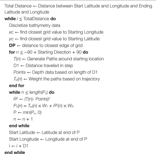
Algorithm 1. LSE/TBN Algorithm.

Acquired depth data are smoothed over time to handle sensor noise and hysteresis. Some of the errors are a result of the fixed angle of the altimeter, causing altitude measurements to be inaccurate during the ascent portion of the yo-yo trajectory path that gliders execute. These data were smoothed using a SD rejection algorithm (Taylor, 1996). During real-time implementation, we break the deployment into pieces consisting of only the segments when the vehicle is diving. These segments are then concatenated to reconstruct the actual path. This implementation method allows for computation to occur during each ascent along the path.

Within Algorithm 1, path options are generated by sweeping the area around the starting location to generate 180 different path options, generating one path option for every compass degree from −90° of the expected direction to +90° of the expected direction. Equations (7a–9b) describe how this is done. First, the point (x, y) is translated to the origin (x_o, y_o).

$x_o=|x-startlong|$ (7a)

$y_o=|y-startlat|$ (7b)

Then, using a rotation formula, the points are rotated about (x′, y′).

$xa=cos(\theta )\times x_o+sin(\theta )\times y_o$ (8a)

$ya=-sin(\theta )\times x_o+cos(\theta )\times y_o;$ (8b)

Each point is then sent back (translated back) to its original location by adding it to the original point (x, y).

$x^{\prime }=xa+startlong$ (9a)

$y^{\prime }=ya+startlat$ (9b)

The length of each possible segment is chosen by picking the closest point of the bathymetric grid to the startlat and startlong. This keeps the step size lengths between 0.0001° and 0.0008°, which is less than or equal to the resolution of the SCCOOS bathymetric maps for each step. The expected direction to initialize the iterative algorithm is taken to be the azimuth from the projected trajectory. An example of the generated path options can be seen in Figure 4. Each path segment length is computed using the Haversine formula. Using this length, we determine the number of data points (DP) within the segment.

FIGURE 4

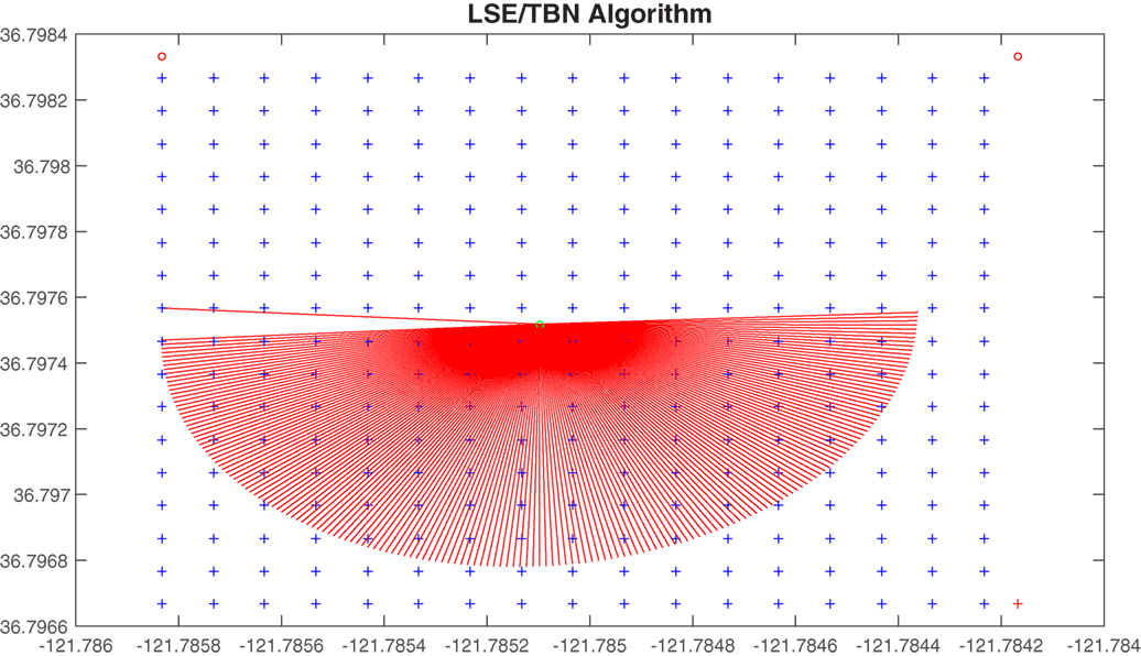
Figure 4. The 180 path options generated around the start latitude and longitude by the LSE/TBN Algorithm.

A linear least-squares approximation is used to compute the error for each path segment between the measured water depth values and an interpolated bathymetric map. The linear least-squares method solves an over-determined system by minimizing the error of the data points to a given line, f(x) = m × x + b, as shown in equation (10).

$R^2={\displaystyle \sum _{i=1}^n}{[y_i-f(x_1,x_2,x_3\mathrm{\dots }{x}_n)]}^2$ (10)

The R² values are normalized between 0 and 1 to provide a weighting for each path segment.

Given the prescribed trajectory, we additionally assign a weight (T_w) to each path segment, based on how close the azimuth is to the initially prescribed trajectory. Assume the prescribed trajectory has an azimuth of 92° from starting point to goal location. The computed path segments then have an azimuth range from 1° to −1°. We assign the preferred direction a value of T_w = 90² and decrease as the segments diverge away from this direction. Thus, an azimuth of 92 would have a weight of T_w = 90², an azimuth of 91 or 93 would have a weighting of T_w = 89², an azimuth of 2 would have a weighting of T_w = 1², etc. The path segments at each epoch are then weighted using the weighting function $T_{w_i}$ shown in equation (11).

$T_{w_i}=1-[(T_{w_i}-min(T_w)/(max(T_w)-min(T_w)]$ (11)

Since $T_{w_i}$ is maximized about the trajectory, it is normalized between 0 and 1 and then subtracted from one to get a minimization criterion.

Finally, a path segment is chosen based on the cost function shown in equation (12). The parameter α is initially set to 0.5 and seeds the algorithm. Altering α allows for emphasizing a preferred heading, e.g., close to the compass heading between the start location and goal location, in regions of minimal bathymetric relief, regions where multiple path segments have identical R² values from the least-squares optimization. As the bathymetric relief approaches zero over the path, α → 1 since the R² values for all paths will approach equality and will not contribute meaningful information to the optimization criterion.

$P_o=T_{w_i}\times \alpha +R^2\times (1-\alpha )$ (12)

Since both T_wi and R² are normalized between zero and one, the weighting factors also stay between zero and one so that neither T_wi nor R² dominate.

The algorithm then initializes the end of the chosen path segment as the new start point, and the process repeats itself until it has utilized all of the available depth data. Further details are presented in Stuntz et al. (2015).

5. Field Experiments

Hundreds of glider missions have been successfully completed off the California coast over the last few years by the University of Southern California CINAPS team (Smith et al., 2010b). For this paper, we utilize data gathered from multiple deployments of Slocum gliders in both Monterey Bay and off the coast of Los Angeles, CA, USA. These data are used to validate the proposed methods to better reconstruct executed trajectories for science analysis and provide better real-time localization while underwater. Commonly, glider trajectories are represented as straight lines underwater by connecting adjacent surfacing locations. The fact is that glider motion is hardly a straight line, as they are continually moved underwater by ocean currents and continual correction with poor navigation systems. The proposed method will provide better mission planning, navigation, and trajectory reconstruction, thus enabling a clearer understanding and contextualization of the data that these vehicles collect.

The experiments in this study were conducted in southern California between July 14 and August 3, 2011 and in Monterey Bay during October 2010. During these times, multiple gliders were deployed that were executing predefined sampling missions and yo-yoing between 2 and 100 m. Further details of these standard missions can be found in Smith et al. (2011a,b). From all of the surfacing locations during the mission executions, we selected those where the subsequent surfacing hit a waypoint. Thus, we selected the dives for which we knew the start location at the surface L, the desired waypoint W_i, the aiming point A_i, and the actual surfacing location S of the vehicle for each segment examined. For southern California, these selected mission segments comprise 34 surfacing events over a span of 21 days. For Monterey Bay, we present one mission demonstrating the proposed TBN algorithm.

6. Unscented Kalman Filter and Ocean Model Prediction Results

For each of the 34 missions considered in the SCB, Figure 5 displays the surfacing error (distance between the desired waypoint and the actual surfacing location) versus the length of the trajectory. Note the linear trend of the data; the longer the glider dead reckons underwater, the greater is the surfacing error. Given that the surfacing error is directly correlated with the distance that the vehicle traveled underwater, we normalize this by use of equation (13) for an equivalent comparison across all 34 missions.

${\text{Error}}_{\text{Normalized}}=\frac{d_g(S,W_i)}{d_g(L,W_i)}$ (13)

FIGURE 5

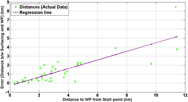
Figure 5. A plot of the absolute surfacing error (in km) versus the length of the prescribed trajectory for the actual field trials.

Here d_g (x, y) is the geographical distance between x and y. Figure 6 displays a heat-map surface plot of this normalized surfacing error within the SCVB for each of the 34 actual surfacing instances. Regions in blue indicate small error, while red regions are indicative of large error. The stars represent the waypoints that the two gliders were trying to achieve. The heat map is computed using a cubic interpolation of the 34 data points.

FIGURE 6

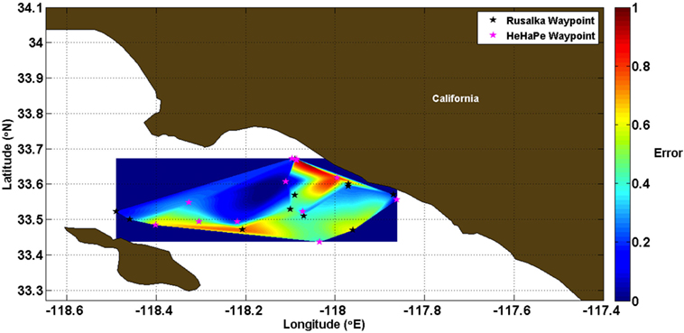
Figure 6. A heat-map surface plot representing the normalized error between the surfacing location and the prescribed waypoint for the actual field trials.

Comparing these errors with water depth, as shown in Smith et al. (2013), we note that the largest errors occur near shore and in the shelf-break portion of the region. These large errors are attributed to the following:

1. Regional forcing drives upwelling across the shelf and creates strong and complex currents in the shelf region, which cannot be modeled well.

2. Two of the northernmost waypoints are less than 1 km apart and are used as a holding pattern between missions. Since the glider must travel by executing an integer number of yos, overshooting the waypoint is likely due to the short baseline distance, the normalized error for geographically close waypoints.

We implemented our developed UKF model to execute all 34 missions using the ocean current predictions from ROMS for the respective day and time of actual execution. Figure 7 displays the surfacing error versus the length of the trajectory for these simulations. The linear trend is not as evident in Figure 7 as previously seen in Figure 5, with much more dispersion in the shorter length missions. Figure 8 displays a heat-map surface plot of this normalized surfacing error within the deployment region for each of the 34 simulated surfacing instances. Regions in blue indicate small error, while red regions are indicative of large error. A normalized error of value >1 indicates a surfacing error greater than the length of the prescribed trajectory. The stars represent the waypoints that the two gliders were trying to achieve. The heat map is computed using a cubic interpolation of the 34 data points.

FIGURE 7

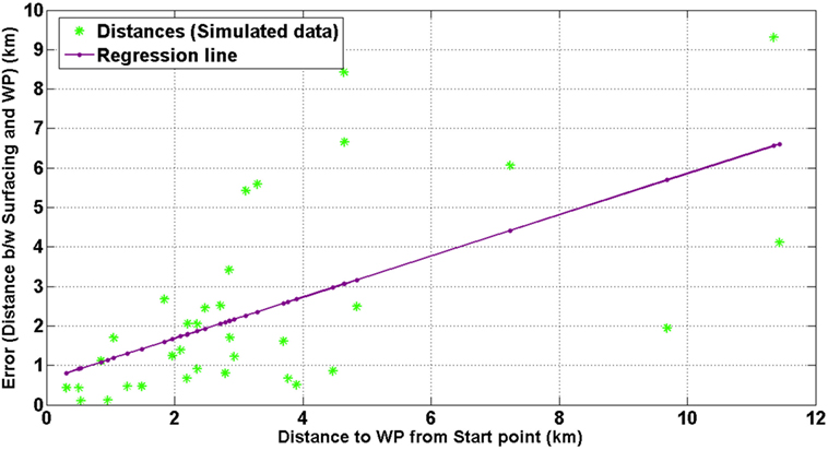
Figure 7. A plot of the absolute surfacing error (in km) versus the length of the prescribed trajectory for the simulated trials.

FIGURE 8

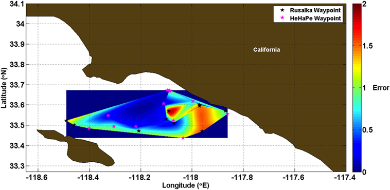
Figure 8. A heat-map surface plot representing the normalized error between the surfacing location and the prescribed waypoint for the simulated trials.

Here, the largest errors are seen directly along the shelf break, a region where the bathymetry changes rapidly as you move toward shore. Note that the scale is different from Figure 6, with the error along the shelf break >1; the surfacing error was larger than the actual length of the prescribed trajectory. It is understandable that a model would have trouble predicting currents in this complex region.

A detailed comparison of these results is presented in Smith et al. (2013), and shows a good match between model predictions and the results of field trial validation for a small region within the SCB. This demonstrates the utility of ocean model predictions within our proposed UKF framework for mission planning and navigation in a coastal region. We note that with just this method, error still exists in the surfacing location. Hence, there is a need for a localization method to determine the actual path that the glider followed.

6.1. Terrain-Based Navigation Results

6.1.1. Monterey Bay Deployment

We demonstrate the effectiveness in localization and path reconstruction of our TBN algorithm on a glider deployment in Monterey Bay, CA, USA, executed during the Monterey Bay Aquarium Research Institute CANON experiments in October 2010 (Chavez, 2010). The deployment region is focused on the northern shelf in Monterey Bay, referred to as the algal bloom incubator. The terrain in this region is varied, and the bathymetry maps are of high resolution. The Glider He Ha Pe (Smith et al., 2010b) was deployed in Monterey Bay in October 2010. Its start position was (36.8431, −121.9204), and it was headed for (36.8097, −121.9041). The actual final surfacing location was (36.8415, −121.8694), a ~4.7-km error in surfacing location. The vehicle traveled a straight line distance of approximately 4.5377 km from its initial position to its ending position. The deployment can be seen in Figure 9. Given the drastic difference in prescribed surfacing location and actual surfacing location, this mission is an excellent candidate for demonstrating our method. The Glider He Ha Pe started at the yellow pin, as shown in Figure 9. The glider surfaced at the green pin but was attempting to head toward the red pin, as shown in Figure 9. Note that the glider surfaced at the location that it thought was the prescribed waypoint. Thus, we see a navigational error in the on-board INS of approximately 4688 m. The glider actually traversed an area with a depth relief of less than 0.4% with raw, recorded depth data showing a relief of approximately 1.7%.

FIGURE 9

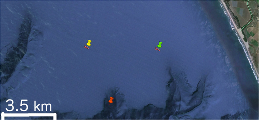
Figure 9. The start position (yellow), goal location (red), and the actual ending position (green) of a glider mission in Monterey Bay, CA, USA. Image courtesy of Google Earth.

Applying the LSE/TBN Algorithm to the chosen trajectory in Monterey Bay, CA, USA, we see a difference between the predicted surfacing location and the actual surfacing location of 55 m. This is the total navigation error over the entire 4.54-km trajectory. The algorithm utilized a weighting factor (α) of 0.5. Figure 10 shows the path computed by the LSE/TBN Algorithm. For this path, the LSE/TBN Algorithm iterated 69 times. A top-down view of the computed trajectory is presented in Figure 11.

FIGURE 10

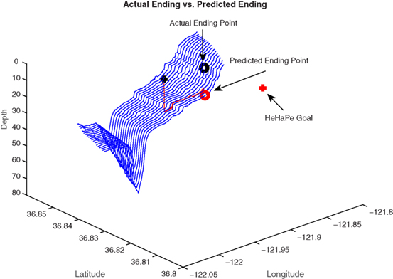
Figure 10. Final results comparing the predicted ending point and the actual ending point. The prescribed goal location is also plotted, demonstrating more than 4000-m dead-reckoning error.

FIGURE 11

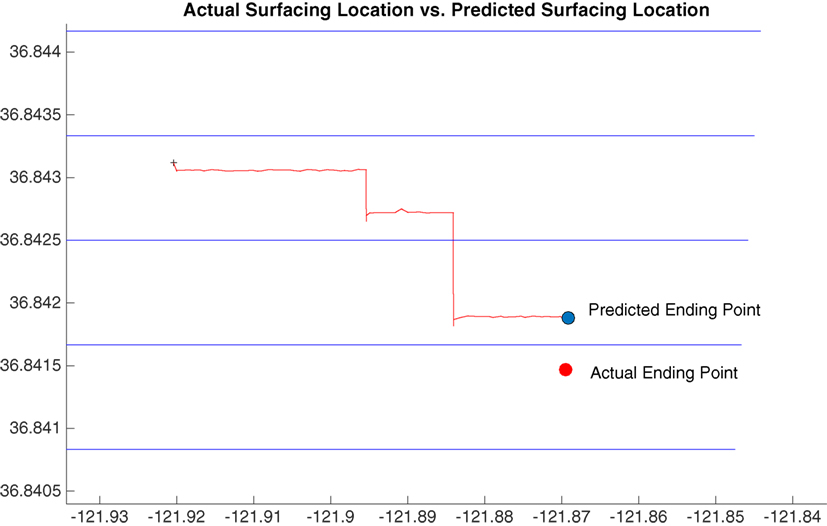
Figure 11. A plot of the actual path followed by the glider as computed by the LSE/TBN Algorithm.

The predicted path is laid over the bathymetry map and presented in Figure 10. Here, we show the actual ending point, predicted ending point, and initial goal. The path followed rises approximately 20 m over a length of 4565.7 m. This is an overall depth relief of approximately less than 0.5%. The distance actually traveled was 4537 m, a difference of 29 m (0.6% error) from the predicted distance traveled. The distance between the actual surfacing location and the predicted surfacing location was 55 m. Some of these errors may be attributed to the drift a glider experiences as it sits on the surface waiting for a GPS fix. Further details and analysis are presented in Stuntz et al. (2015).

6.1.2. Southern California Bight Results

Further validation of the proposed TBN algorithm was demonstrated by examining multiple missions from the Southern California Bight glider missions that were presented in Section 3. We examined 8 of the 34 missions, which occurred in those regions where the ocean model prediction algorithm demonstrated poor results, shallow water, and across the shelf break where there is significant bathymetric relief. The locations of the selected missions overlaid on a bathymetric heat map are presented in Figure 12. Here, red is shallow and blue is deep; the white stars identify the starting location for each mission examined. The results of the TBN algorithm applied to these missions are presented in Table 1. Here, the first column presents the overall length of the path given by our TBN algorithm. The second column provides the prescribed path length as the straight-line distance between start and goal waypoints. The third column gives the distance between the actual surfacing location and the predicted surfacing location given by our TBN algorithm. The fourth column presents the distance between the predicted surfacing location from our TBN algorithm and the actual goal waypoint. The final column displays the distance between the actual goal waypoint and the actual surfacing location of the glider during field trials. Note that during the field trials, the glider was not executing any of the algorithms proposed in this manuscript; hence, it was only relying on dead-reckoning navigation, and the actual surfacing location was not biased or affected by the proposed methods. Figure 13 displays the surfacing error versus the length of the trajectory for these simulations. We note that there is no noticeable trend to these data, with predicted surfacing errors seemingly not dependent upon distance traveled as was the case shown in Figure 5. Most noticeably is a similar error in navigation for paths of 600 and 2500 m. This similarity is a result of the TBN algorithm depending primarily upon the resolution of the underlying bathymetry map, which is 0.0008° or approximately 88 m at the latitude of southern California where the missions were executed. The results from the SCB compare well with those presented for the Monterey Bay data set. This demonstrates the ability of our proposed TBN method to augment the UKF Algorithm for a hybrid algorithm for mission planning and localization to enable persistent operations.

FIGURE 12

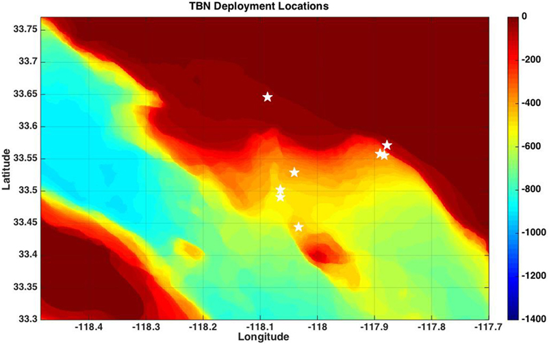
Figure 12. The locations of the eight missions examined with the TBN algorithm overlaid on a bathymetric heat map of the SCB.

TABLE 1

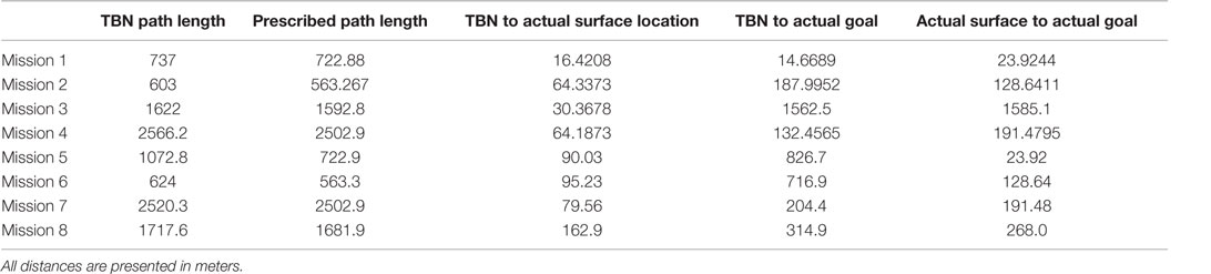
Table 1. Results of applying the TBN Algorithm to multiple missions in the Southern California Bight.

FIGURE 13

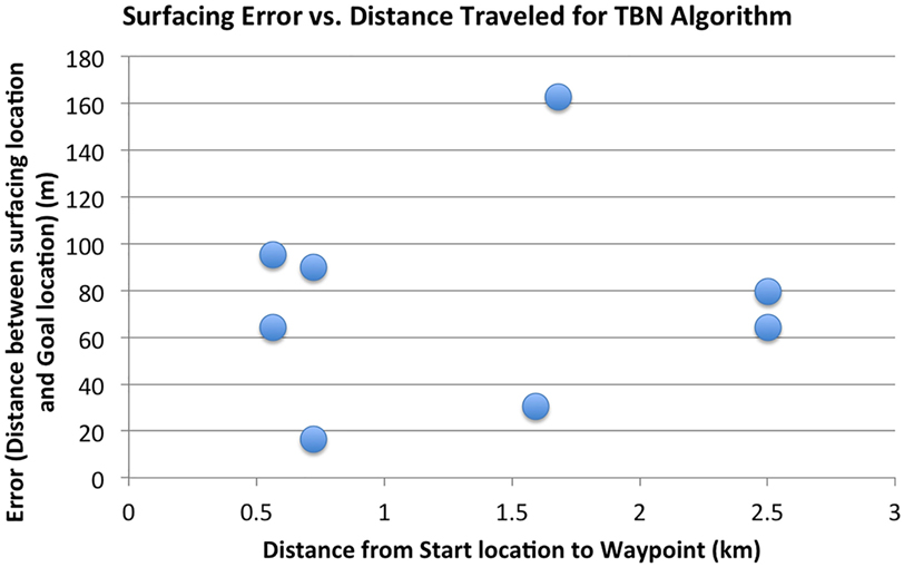
Figure 13. A plot of the TBN predicted surfacing error in meters versus the length of the prescribed trajectory in kilometers.

7. Combining Priors and Predictions

We have presented two methods for aiding underwater gliders to increase navigational accuracy, as well as reconstruct the traversed path after execution. The ocean model prediction method utilizes predictions to aid in plan execution in the uncertain ocean environment. The terrain-based algorithm utilizes priors in the form of bathymetry maps to accurately plot the traversed path of the vehicle while underway. Each method has shown to increase overall accuracy for navigation and the ability of gliders to reach the designated waypoint. However, each method demonstrates poor results over a subset of the experimental domains that are complimentary to one another. Ocean model predictions are not able to predict the currents well over areas of large bathymetic relief, and the accuracy of the model degrades over time. Terrain-based navigation demonstrates excellent results in areas of significant bathymetic relief, and accuracy improves over time by reducing the number of possible locations of the vehicle given the bathymetric history.

In this section, we present Algorithm 2, which combines both approaches. By the design, we rely on the accuracy of the ocean model predictions over short periods of time at the beginning of plan/mission execution and augment this with our proposed TBN method, which performs well in the areas with poor model predictions and maintains high accuracy over long periods of time. Additionally, we utilize each method to provide estimation bounds for the other to maintain a robust navigation solution. The primary contribution of this proposed combined algorithm is to provide low-power, persistent vehicles with an energy-efficient and accurate navigation solution. The proposed technique can be executed on-board gliders during mission execution and will significantly aid in keeping them out of high-risk areas, e.g., shipping lanes. Additionally, the TBN portion of the algorithm is able to track deviations from the UKF predicted mission plan and force surfacing when a threshold error is exceeded. This combined implementation will enable better trajectory tracking by prescribing a surfacing for a GPS fix when necessary, thus maximizing data collection while minimizing time on the surface.

ALGORITHM 2

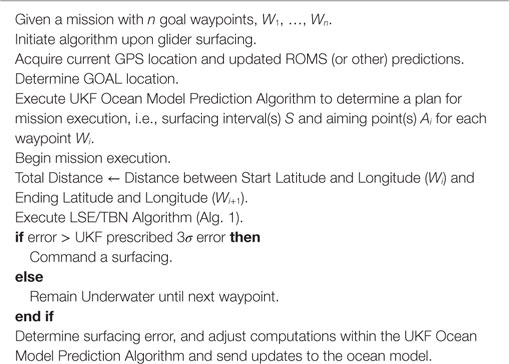
Algorithm 2. UKF Ocean Model and TBN Combined Algorithm.

Given the method of locomotion for an underwater glider, slow velocities and reduced controllability, the following hybrid algorithm is not intended to provide a means for in situ mission adaptation. The UKF Algorithm functions to provide mission planning and reduce navigational error through the use of ocean model predictions. The TBN Algorithm functions to estimate the position of the glider during mission execution to ensure the vehicle does not drift too far off course. Additionally, the TBN Algorithm provides a method to reconstruct the actual executed path of the vehicle.

In the design of Algorithm 2, we utilize the predictions from the ocean model to provide an a priori plan for mission execution, determining aiming points A_i for each waypoint W_i along with potential surfacing locations within the prescribed mission that meet the desired surfacing interval time or maintain a prescribed error bound as described in Section 3; see Smith et al. (2012) for further details. In previous work, the UKF Ocean Model Prediction Algorithm maintained an upper bound on navigational error by implementing frequent surfacing to acquire a GPS fix. Here, we are able to relax this constraint by incorporating the LSE/TBN Algorithm to keep navigation error bounded while the vehicle is underway. This enables longer duration segments underwater, as the glider is free to continue a segment as long as the prescribed navigational error is not violated. Once a prescribed time epoch has elapsed, or a deviation from the prescribed path exceeds a set threshold, the glider is commanded to surface. This method enables safer mission execution coupled with more time for data collection. For each segment of the prescribed path, the aiming point A_i from the UKF Algorithm is used as the initial compass heading to seed Algorithm 1, and this algorithm is run continuously as data are collected during mission execution.

The combined Ocean Model and TBN Algorithm presented in Algorithm 2 were implemented on the same 8 SCB missions used for validation of the TBN Algorithm presented in Section 1. The UKF Ocean Model Prediction Algorithm provided (1) the aiming point A_i for each of the mission segments, which was used as the compass heading to seed the TBN Algorithm and (2) proposed surfacing locations along the path based on an estimated navigational error. Of the eight total missions, the UKF Algorithm prescribed an additional surfacing location for only Missions 4 and 7. This surfacing interval was prescribed for 2 h, based on the predicted currents from ROMS in the area and the uncertainty computed by the UKF Algorithm. Upon execution of Algorithm 2, the proposed additional surfacing locations for Missions 4 and 7 were not requested or implemented since the navigational error never exceeded the prescribed 3σ bound of 600 m based on the TBN Algorithm estimation of location over the duration of the trajectory. However, during Mission 3, the glider was prescribed to surface less than 1 h into the mission since the computed deviation from the prescribed path based on the TBN Algorithm, exceeded the prescribed 3σ bound of 600 m.

As the data used to execute these simulations were the same in situ collected data used to test the TBN Algorithm in Section 4, the performance results from the TBN portion of Algorithm 2 are the same as those listed in Table 1. We did observe slight differences in the computed path given by Algorithm 2 compared to the results by just applying Algorithm 1. These differences were observed during the initial portion of the trajectory, within the first one to three iterations of executing the TBN portion of Algorithm 2. The observed difference is a result of using the azimuth between the start and goal waypoint for Algorithm 1 and the aiming point A_i for Algorithm 2 as the initial compass headings to seed the TBN Algorithm. As pointed out, this did not have an effect on the overall accuracy of the method, as over the length of the paths, the TBN Algorithm was able to converge to the same result.

Given the experience of multiple implementations of the UKF Ocean Model Prediction Algorithm over many glider missions, it is possible, but unlikely, that the predicted initial compass heading supplied to Algorithm 2 may be quite different than the azimuth from prescribed start waypoint to prescribed goal waypoint, e.g., difference >90°. Further experiments are required to analyze the sensitivity of Algorithm 2 to the initial compass heading and are the focus of future work. Additionally, field experiments are planned to validate the promising results shown through these simulated field trials.

8. Conclusion

In this paper, we examined multiple missions that were executed by autonomous gliders in coastal regions in southern California. The results from the field experiments were compared with simulations of the same missions in a UKF that integrated ROMS current predictions and a TBN algorithm for determining location and traversed path underwater. We found that incorporating ocean model predictions does improve navigational accuracy and plan execution; however, this method alone neither produces reliable predictions over long periods of time nor in regions of complex current structure, e.g., shelf break. We found excellent results for localization and path reconstruction in the shallow and shelf-break region using the proposed TBN algorithm. Contrary to the ocean model prediction incorporation, the LSE/TBN Algorithm has an upper bound on error based on the resolution of the underlying bathymetry map, regardless of the distance or time traveled. In the majority of areas within the deployment region studied, ROMS provided a prediction of the ocean current that corresponded well with field experiment results. This information can be used to increase the utility of the deterministic model predictions by understanding what regions actually do have unpredictable currents.

The LSE/TBN Path Estimation algorithm provides a real-time path estimator that provides an improved estimation of the route the glider took over the course of a deployment over existing dead-reckoning solutions. This improved path estimation provides a better understanding of the position of the glider for scientists that utilize the instruments on the glider. It is clear that a combination of the proposed methodologies will provide increased navigational accuracy in this oceanic region for autonomous gliders by forcing a surfacing when a glider veers too far away from the prescribed path.

This paper shows the feasibility of a combined approach to mission planning and execution for autonomous gliders to perform persistent monitoring/sampling in coastal ocean regions. Utilizing model predictions for mission planning coupled with a terrain-based navigation while underway has the ability to provide accurate localization estimates for gliders to ~100 m, without the use of high-power sensors such as DVLs or acoustic communications. This error is approximately 1/5th the accuracy previously reported for similar vehicles utilizing dead-reckoning and minimal sensing capabilities (Nicholson and Healey, 2008; Davis et al., 2009; Smith et al., 2010c, 2012, 2013). The proposed, combined methodology provides this bound on navigational accuracy, regardless of trajectory length or mission duration. The primary application of the proposed method is to bound navigational error for gliders during mission execution, thus keeping them out of high-risk areas, such as shipping lanes, and enabling better trajectory tracking by knowing when a GPS fix is necessary to relocalize.

9. Future Work

In this paper, we presented two techniques for operating autonomous gliders for persistent operations. It has been shown that real-time glider navigation accuracy can be increased through the incorporation of ocean model predictions and an Unscented Kalman Filter (UKF) (Smith et al., 2010c, 2012). However, even in this case, the uncertainty grows without bound. In the first step to implement our combined method in a real-time scenario, we utilized it as a means to bound the uncertainty in the UKF. We implemented this algorithm in simulation to demonstrate that we can command a surfacing when the path deviation exceeds a prescribed value. We plan to implement our method online and provide a position estimate for the UKF to compare with at each update epoch. We plan to implement this hybrid system onto a pair of autonomous gliders during field trials in the SCB during summer 2016 to compare with a dead-reckoning solution in situ.

Given the existing research presented earlier on the use of particle filters for TBN for underwater vehicles, we plan to develop a particle filter method for integration within the existing ocean model and UKF framework. This will hopefully provide an online set of navigation tools for accurate localization for underwater vehicles that operate for long-duration missions.

The study presented here serves as an initial investigation into the comparison of actual ground truth with ocean model predictions. Future work will expand on this effort to include more field trials over longer time periods, as well as to compare other output variables of the model, e.g., salinity, temperature, and chlorophyll, with those measured by the vehicle(s). Additionally, we intend to examine field trials conducted during the same time period over multiple years to examine the ability of the model to predict seasonal and annual variability in the structure of the ocean currents in southern California.

Further research includes examining multiple other glider trajectories from USC CINAPS (Smith et al., 2010b) to assess algorithm sensitivity, and formalizing and proving the proposed methodology for other AUVs, specifically propeller-driven vehicles such as the YSI EcoMapper AUV (YSI Incorporated, 2016). The majority of deployments of these vehicles is much shorter than that of the gliders and will provide a good case study for a lower bound on the applicability of our methods. Also, we will use a YSI EcoMapper vehicle, which includes a 10-beam DVL, to provide accurate ground truth to further benchmark the proposed method. The proposed terrain-based navigation method is a complement to other localization systems present for any vehicle. We see this as augmenting existing systems, as well as bounding the inherent errors of other navigation systems, i.e., filtering methods.

Note that the presented method is virtually model free, relying only on the vehicle speed for matching measured water depth values with bathymetric maps. In general, the exact vehicle velocity is not known but approximated and well-bounded. We propose to extend the current method by iterating through reasonable velocities and optimizing over potential trajectory options to determine the best match with gathered data. This will also provide information on the actual speed of the vehicle that can be used in other analyses.

As eluded to earlier, many AUV deployments are routine missions carried out in bounded and known locations. We propose to utilize this prior knowledge to improve localization in uncertain environments by updating existing bathymetric maps. Amassing depth data over a deployment region will significantly improve localization for future missions. SCCOOS and the University of Southern California have amassed a large amount of depth data off the coast of Central and Southern California. By combining data of previous missions, better bathymetric maps can be developed and utilized in a TBN framework to augment navigation methods utilized on many vehicles.

Author Contributions

All authors had equal contribution toward the authorship of this manuscript.

Conflict of Interest Statement

The authors declare that the research was conducted in the absence of any commercial or financial relationships that could be construed as a potential conflict of interest.

Funding

AS was supported in part by a Fort Lewis College undergraduate research grant. RS was supported in part by a Byron Dare Junior Faculty Award.

References

Alvarez, A., Caiti, A., and Onken, R. (2004). Evolutionary path planning for autonomous underwater vehicles in a variable ocean. IEEE J. Oceanic Eng. 29, 418–429. doi: 10.1109/JOE.2004.827837

CrossRef Full Text | Google Scholar

Anderson, D. M., Glibert, P. M., and Burkholder, J. M. (2002). Harmful algal blooms and eutrophication: nutrient sources, composition, and consequences. Estuaries 25, 704–726. doi:10.1007/BF02804901

CrossRef Full Text | Google Scholar

Anonsen, K. B., and Hallingstad, O. (2006). “Terrain aided underwater navigation using point mass and particle filters,” in Proceedings of the IEEE/ION Position Location and Navigation Symposium, Coronado/San Diego, CA.

Google Scholar

Anonsen, K. B., and Hallingstad, O. (2007). “Sigma point kalman filter for underwater terrain-based navigation,” in Proceedings of the 7th IFAC Conference on Control Applications in Marine Systems (Grand Hotel Elaphusa, Croatia: Elsevier), 106–110.

Google Scholar

Chavez, F. (2010). Canon: Controlled, Agile, and Novel Observing Network. Available at: http://www.mbari.org/canon

Google Scholar

Davis, R. E., Leonard, N. E., and Fratantoni, D. M. (2009). Routing strategies for underwater gliders. Deep Sea Res. Part II Top. Stud. Oceanogr. 56, 173–187. doi:10.1016/j.dsr2.2008.08.005

CrossRef Full Text | Google Scholar

Davis, R. E., Ohman, M. D., Rudnick, D. L., Sherman, J. T., and Hodges, B. (2008). Glider surveillance of physics and biology in the southern California Current System. Limnol. Oceanogr. 53, 2151–2168. doi:10.4319/lo.2008.53.5_part_2.2151

CrossRef Full Text | Google Scholar

Ferrari, R. (2011). Ocean science. A frontal challenge for climate models. Science 332, 316–317. doi:10.1126/science.1203632

CrossRef Full Text | Google Scholar

Flenniken, W., Wall, J., and Bevly, D. (2005). “Characterization of various IMU error sources and the effect on navigation performance,” in Proceedings of the 18th International Technical Meeting of the Satellite Division of the Institute of Navigation ION GNSS 2005 (Long Beach, CA: Long Beach Convention Center), 967–978.

Google Scholar

Fulton-Bennett, K. (2005). Canyons, Currents, and Algal Blooms – How Monterey Canyon Influences the Growth of Microscopic Marine Algae. Moss Landing, CA: Monterey Bay Aquarium Research Institute. Available at: http://www3.mbari.org/news/homepage/2005/ryan-blooms.html

Google Scholar

Garau, B., Alvarez, A., and Oliver, G. (2005). “Path planning of autonomous underwater vehicles in current fields with complex spatial variability: an {A}* approach,” in Proceedings of the IEEE International Conference on Robotics and Automation, Barcelona.

Google Scholar

Godin, M. A., Bellingham, J. G., Rajan, K., Chao, Y., and Leonard, N. E. (2006). “A collaborative portal for ocean observatory control,” in Proceedings of the Marine Technology Society/Institute of Electrical and Electronics Engineers Oceans Conference, Boston, MA.

Google Scholar

Golden, J. P. (1980). “Terrain contour matching (TERCOM): a cruise missile guidance aid,” in 24th Annual Technical Symposium (San Diego, CA: International Society for Optics and Photonics), 10–18.

Google Scholar

Griffiths, G., Jones, C., Ferguson, J., and Bose, N. (2007). Undersea gliders. J. Ocean Technol. 2, 64–75.

Google Scholar

Gustafsson, F., Gunnarsson, F., Bergman, N., Forssell, U., Jansson, J., Karlsson, R., et al. (2002). Particle filters for positioning, navigation, and tracking. IEEE Trans. Signal. Process. 50, 425–437. doi:10.1109/78.978396

CrossRef Full Text | Google Scholar

Hollinger, G. A., Englot, B., Hover, F., Mitra, U., and Sukhatme, G. S. (2012). “Uncertainty-driven view planning for underwater inspection,” in Proceedings of the IEEE International Conference on Robotics and Automation (St. Paul, MN), 4884–4891.

Google Scholar

Horner, R. A., Garrison, D. L., and Gerald, F. (1997). Harmful algal blooms and red tide problems on the U.S. west coast. Limnol. Oceanogr. 42, 1076–1088. doi:10.4319/lo.1997.42.5_part_2.1076

CrossRef Full Text | Google Scholar

Huster, A., and Rock, S. M. (2003). “Relative position sensing by fusing monocular vision and inertial rate sensors,” in Proceedings of the 11th International Conference on Advanced Robotics {(ICAR’03)}, Vol. 3 (Coimbra: IEEE), 1562–1567.

Google Scholar

Jones, B. H., Noble, M. A., and Dickey, T. D. (2002). Hydrographic and particle distributions over the Palos Verdes Continental Shelf: spatial, seasonal and daily variability. Cont. Shelf Res. 22, 945–965. doi:10.1016/S0278-4343(01)00114-5

CrossRef Full Text | Google Scholar

Julier, S. J., and Uhlmann, J. K. (2004). Unscented filtering and nonlinear estimation. Proc. IEEE 92, 401–422. doi:10.1109/JPROC.2003.823141

CrossRef Full Text | Google Scholar

Kinsey, J. C., Eustice, R. M., and Whitcomb, L. L. (2006). “A survey of underwater vehicle navigation: recent advances and new challenges,” in IFAC Conference of Manoeuvering and Control of Marine Craft, Lisbon.

Google Scholar

Kruger, D., Stolkin, R., Blum, A., and Briganti, J. (2007). “Optimal AUV path planning for extended missions in complex, fast-flowing estuarine environments,” in Proceedings of the IEEE International Conference on Robotics and Automation, Rome.

Google Scholar

Kudela, R., Pitcher, G., Probyn, T., Figueiras, F., Moita, T., and Trainer, V. (2005). Harmful algal blooms in coastal upwelling systems. Oceanography 18, 184–197. doi:10.5670/oceanog.2005.53

CrossRef Full Text | Google Scholar

Lagadec, J. (2010). Terrain Based Navigation Using a Particle Filter for Long Range Glider Missions – Feasibility Study and Simulations. La Spezia: Master’s thesis, ENSIETA Ecole Nationale Superieure DIngenieurs.

Google Scholar

Mancho, A. M., Hernández-García, E., Small, D., Wiggins, S., and Fernández, V. (2008). Lagrangian transport through an ocean front in the Northwestern Mediterranean Sea. J. Phys. Oceanogr. 38, 1222–1237. doi:10.1175/2007JPO3677.1

CrossRef Full Text | Google Scholar

Nicholson, J. W., and Healey, A. J. (2008). The present state of autonomous underwater vehicle (AUV) applications and technologies. Mar. Technol. Soc. J. 42, 44–51. doi:10.4031/002533208786861272

CrossRef Full Text | Google Scholar

Ono, M., and Williams, B. C. (2008). “An efficient motion planning algorithm for stochastic dynamic systems with constraints on probability of failure,” in Proceedings of the Twenty-Third AAAI Conference on Artificial Intelligence, Chicago, IL.

Google Scholar

Paley, D., Zhang, F., and Leonard, N. (2008). Cooperative control for ocean sampling: the glider coordinated control system. IEEE Trans. Control. Syst. Technol. 16, 735–744. doi:10.1109/TCST.2007.912238

CrossRef Full Text | Google Scholar

Pereira, A. A., Binney, J., Hollinger, G. A., and Sukhatme, G. S. (2013). Risk-aware path planning for autonomous underwater vehicles using predictive ocean models. J. Field Rob. 30, 741–762. doi:10.1002/rob.21472

CrossRef Full Text | Google Scholar

Powell, B. S., Arango, H. G., Moore, A. M., Lorenzo, E. D., Milliff, R. F., and Foley, D. (2008). 4DVAR data assimilation in the Intra-Americas Sea with the Regional Ocean Modeling System (ROMS). Ocean Modell. 25, 173–188. doi:10.1016/j.ocemod.2008.08.002

CrossRef Full Text | Google Scholar

Rao, D., and Williams, S. B. (2009). “Large-scale path planning for underwater gliders in ocean currents,” in Proceedings of the Australasian Conference on Robotics and Automation, Sydney.

Google Scholar

Rixen, M., Book, J. W., Carta, A., Grandi, V., Gualdesi, L., Stoner, R., et al. (2009). Improved ocean prediction skill and reduced uncertainty in the coastal region from multi-model super-ensembles. J. Mar. Syst. 78, S282–S289. doi:10.1016/j.jmarsys.2009.01.014

CrossRef Full Text | Google Scholar

SCCOOS. (2009). SCCOOS: Southern California Coastal Observing System. Available at: http://www.sccoos.org

Google Scholar

Schnetzer, A., Miller, P. E., Schaffner, R. A., Stauffer, B., Jones, B. H., Weisberg, S. B., et al. (2007). Blooms of Pseudo-nitzschia and domoic acid in the San Pedro Channel and Los Angeles harbor areas of the Southern California Bight, 2003-2004. Harmful Algae 6, 372–387. doi:10.1016/j.hal.2006.11.004

CrossRef Full Text | Google Scholar

Schofield, O., Kohut, J., Aragon, D., Creed, E., Graver, J., Haldman, C., et al. (2007). Slocum gliders: robust and ready. J. Field Rob. 24, 473–485. doi:10.1002/rob.20200

CrossRef Full Text | Google Scholar

Sekula-Wood, E., Schnetzer, A., Benitez-Nelson, C. R., Anderson, C., Berelson, W., Brzezinski, M., et al. (2009). The Toxin Express: rapid downward transport of the neurotoxin domoic acid in coastal waters. Nature Geosci. 2, 273–275. doi:10.1038/ngeo472

CrossRef Full Text | Google Scholar

Smith, R. N., Chao, Y., Li, P. P., Caron, D. A., Jones, B. H., and Sukhatme, G. S. (2010a). Planning and implementing trajectories for autonomous underwater vehicles to track evolving ocean processes based on predictions from a regional ocean model. Int. J. Rob. Res. 29, 1475–1497. doi:10.1177/0278364910377243

CrossRef Full Text | Google Scholar

Smith, R. N., Das, J., Heidarsson, H., Pereira, A., Cetinić, I., Darjany, L., et al. (2010b). USC CINAPS builds bridges: observing and monitoring the Southern California Bight. IEEE Rob. Autom. Mag. 17, 20–30. doi:10.1109/MRA.2010.935795

CrossRef Full Text | Google Scholar

Smith, R. N., Kelly, J., Chao, Y., Jones, B. H., and Sukhatme, G. S. (2010c). “Towards improvement of autonomous glider navigation accuracy through the use of regional ocean models,” in Proceedings of the 29th International Conference on Offshore Mechanics and Arctic Engineering (Shanghai: ASME), 597–606.

Google Scholar

Smith, R. N., Kelly, J., Nazarzadeh, K., and Sukhatme, G. S. (2013). “An investigation on the accuracy of regional ocean models through field trials,” in Proceedings of the IEEE International Conference on Robotics and Automation, Karlsruhe.

Google Scholar

Smith, R. N., Kelly, J., and Sukhatme, G. S. (2012). “Towards improving mission execution for autonomous gliders with an ocean model and Kalman filter,” in Proceedings of the IEEE International Conference on Robotics and Automation (St. Paul, MN), 4870–4877.

Google Scholar

Smith, R. N., Schwager, M., Smith, S. L., Jones, B. H., Rus, D., and Sukhatme, G. S. (2011a). Persistent ocean monitoring with underwater gliders: adapting sampling resolution. J. Field Rob. 28, 714–741. doi:10.1002/rob.20405

CrossRef Full Text | Google Scholar

Smith, R. N., Schwager, M., Smith, S. L., Rus, D., and Sukhatme, G. S. (2011b). “Persistent ocean monitoring with underwater gliders: towards accurate reconstruction of dynamic ocean processes,” in Proceedings of the IEEE International Conference on Robotics and Automation (Shanghai), 1517–1524.

Google Scholar

Stevens, B. L., and Lewis, F. L. (2003). Aircraft Control and Simulation, 2nd Edn. Hoboken, NJ: Wiley-Interscience.

Google Scholar

Stuntz, A., Liebel, D., and Smith, R. N. (2015). “Enabling persistent autonomy for underwater gliders through terrain based navigation,” in OCEANS 2015 – Genova (Genova: IEEE), 1–10.

Google Scholar

Taylor, J. R. (1996). An Introduction to Error Analysis: The Study of Uncertainties in Physical Measurements (Sausalito, CA: University Science Books), 166–168.

Google Scholar

Vu, Q. (2008). JPL: OurOcean Portal. Available at: http://ourocean.jpl.nasa.gov

Google Scholar

Webb Research Corporation. (2008). Slocum Glider. Available at: http://www.webbresearch.com/slocumglider.aspx

Google Scholar

Whitcomb, L., Yoerger, D., Singh, H., and Howland, J. (1999). “Advances in underwater robot vehicles for deep ocean exploration: navigation, control, and survey operations,” in Proceedings of the Ninth International Symposium of Robotics Research (Snowbird, UT: Springer-Verlag), 439–448.

Google Scholar

Witt, J., and Dunbabin, M. (2008). “Go with the flow: optimal path planning in coastal environments,” in Proceedings of the 2008 Australasian Conference on Robotics & Automation (ACRA 2008), eds J. Kim and R. Mahony (Canberra, ACT).

Google Scholar

YSI Incorporated, Y. (2016). YSI EcoMapper. Available at: http://www.ysisystems.com/productsdetail.php?EcoMapper-Autonomous-Underwater-Vehicle-9

Google Scholar

Zhang, Y., Bellingham, J. G., Ryan, J. P., Kieft, B., and Stanway, M. J. (2013). “Two-dimensional mapping and tracking of a coastal upwelling front by an autonomous underwater vehicle,” in 2013 OCEANS – San Diego (San Diego: IEEE), 1–4.

Google Scholar