On the Dynamics and Control of Free-floating Space Manipulator Systems in the Presence of Angular Momentum

Introduction

In the coming years, on orbit robotic systems will have a large impact in a wide variety of operations encountered in space exploration. Their ability to execute tasks in environments, which pose great dangers to human life minimizes the risk that astronauts face and increases mission productivity. Space robotic manipulators include a spacecraft (base) with one or more robotic manipulators mounted on it, see Figure 1A. Examples of such systems are the ETS–7 (Oda, 1999), the Orbital-Express (Ogilvie et al., 2008), and more recently, the DEOS (Reintsema et al., 2010).

FIGURE 1

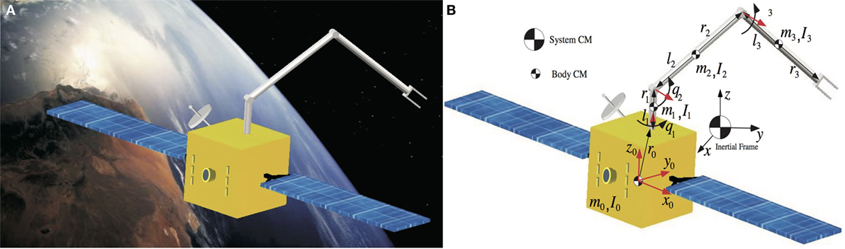
Figure 1. (A) A space manipulator system, (B) the spatial free-floating space manipulator systems and definition of its parameters.

The spacecraft can be transferred and oriented arbitrarily in space using thrusters and reaction wheels controlled by the attitude determination and control system (ADCS). The desired end-effector position and orientation is achieved by controlling the joint motors via the manipulator control system. Each of these control systems operates independently. However, due to dynamic coupling, the motion of the end-effector affects the motion of the spacecraft and vice versa. Thus, in the case the end-effector is desired to execute a specific motion, it is preferable to turn-off the ADCS since the independent control of the spacecraft can cause undesirable disturbances to the end-effector motion. Then, the system operates in a free-floating mode during which the uncontrolled motion of the spacecraft arises as a result of the dynamic coupling between the spacecraft and the manipulator.

The lack of a fixed base, on which the manipulator is mounted, poses several challenges to the operation and control of free-floating space manipulator systems (FFSMS). Two types of motion control are considered. The first, called spacecraft-referenced end-point motion control, is the mode of control where the end-effector is commanded to move to a location fixed to its own spacecraft. An example is the case where the manipulator is driven to its stewed position. The second, called inertially referenced end-point motion control, is the mode of control where the end-effector is commanded to move with respect to inertial space (Papadopoulos and Dubowsky, 1991a).

Although zero initial system angular momentum is desired before the motion of an FFSMS, due to small collisions with the environment or due to on-off attitude controller inaccuracies, significant amounts of angular momentum tend to accumulate. In general, these accumulated amounts of angular momentum can be absorbed using either thruster jets or momentum control devices (e.g., reaction/momentum wheels, control momentum gyroscopes). However, thrusters by their nature use expendable propellants, limiting system life. Momentum control devices require only electrical power that can be supplied by solar arrays. However, these devices tend to saturate and ultimately, also require use of thrusters for despinning. Thus, the control of an FFSMS, under the presence of angular momentum, and without the use of additional actuators is important and is studied here.

Masutani et al. (1989) have addressed a point-to-point control of the end-effector of an FFSMS with zero angular momentum. They proposed a sensory feedback scheme based on an artificial potential defined in the sensor coordinate frame. Xu and Shum (1991) derived the equations of motion of FFSMS with zero angular momentum in joint and inertial space, applying the Langragian methodology. Based on the dynamic model, a simple linear control scheme was presented for the point-to-point control problem and a globally stable control law was proposed for trajectory tracking applications. Umetani and Yoshida (1989) introduced the free-floating system generalized Jacobian matrix (GJM) and developed a resolved rate and acceleration control method based on it. Caccavale and Siciliano (2001) employed the GJM in solving the inverse kinematics of a free-floating space manipulator. Papadopoulos and Dubowsky (1991a), based on the similarities of the structure of the kinematics and dynamics between fixed base and FFSMS with zero angular momentum, showed that almost any terrestrial fixed base control algorithm can be applied to FFSMS with zero angular momentum, considering some additional conditions. The same researchers, proposed a complete coordinated control method, based on the transposed Jacobian, which can achieve both position and orientation of the end-effector and the spacecraft of an FFSMS with zero initial angular momentum (Papadopoulos and Dubowsky, 1991b).

More recently, Rybus et al. (2015) analyzed a control scheme based on the fixed base Jacobian inverse with the addition of the spacecraft velocity, in order to reduce the complexity caused by the use of the GJM. A non-linear model predictive control method was proposed taking into account the free-floating nature of the system. The results were compared to the ones obtained with the GJM-based controller (Rybus et al., 2017). To synthesize the spacecraft ADCS and the manipulator controller of a space robot, a fixed-structure H_∞ synthesis has been proposed in Dubanchet et al. (2015).

All the previous research was based on the assumption that the system is at rest initially, i.e., the initial momentum of FFSMS is 0. Mathematically speaking, an FFSMS with initial angular momentum is an affine system with a drift term. This term is caused by the angular momentum and complicates the path planning and control of such systems. To date, a limited number of studies have dealt with this issue. Matsuno and Saito (2001) have proposed an attitude control law, considering a planar two-link space robot with initial angular momentum, i.e., a typical example of a 3-state and 2-input affine system with a drift term. Although the controller takes the system to the desired location, the system drifts away due to the non-zero angular momentum (NZAM). Yamada et al. (1995) have presented a path planning scheme for a single arm of an FFSMS, which is equipped with momentum wheels. This method utilizes the angular momentum of the base, without causing its nutation, which occurs unless the final attitude of the base is the same as the initial one. More recently, a trajectory optimization method for systems with non-conserved linear and angular momentum has been proposed (Rybus et al., 2016). Nanos and Papadopoulos (2011) have proposed an approach that identifies workspace areas and required joint motions so that the end-effector can remain fixed despite the NZAM. The same authors have proposed a methodology to avoid the path-dependent dynamic singularities (DS), defined in Papadopoulos and Dubowsky (1993), by carefully choosing the FFSMS initial configuration (Nanos and Papadopoulos, 2012). More recently, they extended this methodology to FFSMS with NZAM (Nanos and Papadopoulos, 2015).

In this paper, the control of FFSMS with NZAM, for motions both in the joint and Cartesian space, is studied. First, the dynamic models in joint and Cartesian space, for FFSMS with NZAM, are derived. It is shown that the NZAM has an effect similar to that of gravity on terrestrial fixed base manipulators. Thus, to compensate for the effect of the NZAM, the application of controllers similar to the ones used for gravity compensation in terrestrial fixed base manipulators is proposed. To confirm the asymptotic stability of the proposed controllers, some structural properties of the dynamic models must be satisfied. It is shown that despite the presence of NZAM, these structural properties are still valid. Thus, the proposed controllers can drive the system in the desired position despite the presence of NZAM. However, the NZAM imposes constraints on the Cartesian position where the end-effector can be driven. Limitations are discussed and the application of the proposed controllers is illustrated by examples.

Dynamics of Free-Floating Space Manipulators

On orbit systems operate in a free-fall environment where during operations the gravitational effects are not absent. However, for motions with time duration shorter than one orbit period, the gravitational torques, as well as the air drag and magnetic torques, are expected to be much smaller with respect to the joint actuator torques, inertia torques, and centrifugal/Coriolis torques (From et al., 2014; Flores-Abad and Crespo, 2015). Thus, most often no external forces act on an FFSMS and, therefore, the motion of the system is governed by the momentum conservation; the effect of the gravity is left out of the equations of motion of FFSMS (Papadopoulos and Dubowsky, 1991a).

In this section, the differential kinematics and the equations of motion of a rigid FFSMS with NZAM are briefly developed. The dynamics of FFSMS under the presence of angular momentum have been studied in Nanos and Papadopoulos (2011). Here, the equations of motions are written in a form suitable for control purposes.

According to the current practice in space, on orbit robotic systems have revolute joints in an open chain configuration. In a free-floating system with a N degrees-of-freedom (DOF) manipulator, there will be N + 6 DOF in total including the DOF of the spacecraft. Here, free-floating systems with a single non-redundant manipulator (N ≤ 6) are considered. In this case, the additional DOF, required for obstacle or singularities avoidance, are obtained by the free motion of the spacecraft. The use of non-redundant manipulators simplifies the mechanical design of such systems and results in a smaller mass system. The system center of mass (CM) does not accelerate, and the system linear momentum is constant. With the further assumption of zero initial linear momentum, the system CM remains fixed in inertial space, and the origin, O, can be chosen to be the system CM, see Figure 1B.

Angular Momentum and Differential Kinematics

First, the conservation of angular momentum and the differential kinematics of an FFSMS in the presence of angular momentum are briefly presented.

The angular momentum h_CM expressed in the inertial frame is constant and is given by:

${\mathbf{\text{h}}}_{\mathbf{\text{CM}}}={\mathbf{\text{R}}}_{\mathbf{0}}\left(\mathbf{\text{ε}},n\right)\left({}^{\mathbf{0}}\mathbf{\text{D}}\left(\mathbf{\text{q}}\right){}^{\mathbf{0}}{\mathbf{\text{ω}}}_{\mathbf{0}}+{}^{\mathbf{0}}{\mathbf{\text{D}}}_{\mathbf{\text{q}}}\left(\mathbf{\text{q}}\right)\dot{\mathbf{\text{q}}}\right)=\text{const}.$ (1)

where ⁰ω₀ is the spacecraft angular velocity, expressed in the spacecraft 0th frame and the N × 1 column-vectors $\mathbf{\text{q}},\dot{\mathbf{\text{q}}}$ represent manipulator joint angles and rates, respectively. The matrix R₀(ε,n) is the rotation matrix between the spacecraft 0th frame and the inertial frame, expressed as a function of the spacecraft Euler parameters ε, n. The 3 × 3 matrix ⁰D is the inertia matrix of the entire system as seen from the system CM, expressed in the spacecraft 0th frame, and as such it is a positive definite symmetric matrix and thus always invertible. The 3 × N matrix ⁰D_q corresponds to the inertia of the system’s moving parts. Both matrices are functions of q, and given in detail in Papadopoulos and Dubowsky (1991a), see Appendix A.

The end-effector linear velocity ${\dot{\mathbf{\text{r}}}}_{\mathbf{\text{E}}}$ and angular velocity ω_E are given by:

${\dot{\mathbf{\text{r}}}}_{\mathbf{\text{E}}}={\mathbf{\text{R}}}_{\mathbf{0}}\left(\mathbf{\text{ε}},n\right)\left({}^{\mathbf{0}}{\mathbf{\text{J}}}_{\mathbf{\text{11}}}\left(\mathbf{\text{q}}\right){}^{\mathbf{0}}{\mathbf{\text{ω}}}_{\mathbf{0}}+{}^{\mathbf{0}}{\mathbf{\text{J}}}_{\mathbf{\text{12}}}\left(\mathbf{\text{q}}\right)\dot{\mathbf{\text{q}}}\right)$ (2)

${\mathbf{\text{ω}}}_{\mathbf{\text{E}}}={\mathbf{\text{R}}}_{\mathbf{0}}\left(\mathbf{\text{ε}},n\right)\left({}^{\mathbf{0}}{\mathbf{\text{ω}}}_{\mathbf{0}}+{}^{\mathbf{0}}{\mathbf{\text{J}}}_{\mathbf{\text{22}}}\left(\mathbf{\text{q}}\right)\dot{\mathbf{\text{q}}}\right)$ (3)

where the matrices ⁰J₁₁, ⁰J₁₂, and ⁰J₂₂ are Jacobian-type matrices of appropriate dimensions, functions of q, and given in detail in Appendix B.

Using the angular momentum conservation, given by Eq. 1, the spacecraft angular velocity ⁰ω₀ can be substituted in Eqs 2 and 3. Then, the vector ${\mathbf{\text{v}}}_{\mathbf{\text{E}}}={\left[\begin{array}{cc}\hfill {\dot{\mathbf{\text{r}}}}_{\mathbf{\text{E}}}^{\text{T}}\hfill & \hfill {\mathbf{\text{ω}}}_{\mathbf{\text{E}}}^{\text{T}}\hfill \end{array}\right]}^{\text{T}}$ is given by Nanos (2015):

${\mathbf{\text{v}}}_{\mathbf{\text{E}}}=\left[\begin{array}{c}\hfill {\dot{\mathbf{\text{r}}}}_{\mathbf{\text{E}}}\hfill \\ \hfill {\mathbf{\text{ω}}}_{\mathbf{\text{E}}}\hfill \end{array}\right]=\mathbf{\text{E}}\left(\mathbf{\text{ε}},n\right)\left({}^{\mathbf{0}}{\mathbf{\text{J}}}_{\mathbf{\text{q}}}\left(\mathbf{\text{q}}\right)\dot{\mathbf{\text{q}}}+{}^{\mathbf{0}}{\mathbf{\text{J}}}_{\mathbf{\text{h}}}{\mathbf{\text{R}}}_{\mathbf{0}}^{\text{T}}\left(\mathbf{\text{ε}},n\right){\mathbf{\text{h}}}_{\mathbf{\text{CM}}}\right)$ (4)

where the 6 × 6 matrix E(ε,n) is given by:

$\mathbf{\text{E}}\left(\mathbf{\text{ε}},n\right)=\left[\begin{array}{cc}\hfill {\mathbf{\text{R}}}_{\mathbf{0}}\left(\mathbf{\text{ε}},n\right)\hfill & \hfill {\mathbf{0}}_{\mathbf{\text{3}}\times \mathbf{\text{3}}}\hfill \\ \hfill {\mathbf{0}}_{\mathbf{\text{3}}\times \mathbf{\text{3}}}\hfill & \hfill {\mathbf{\text{R}}}_{\mathbf{0}}\left(\mathbf{\text{ε}},n\right)\hfill \end{array}\right]$ (5)

where 0_{m × n} is the m × n zero matrix.

Note that in case the end-effector attitude is expressed with the Euler angles θ_E, the following equation can be used:

${\mathbf{\text{ω}}}_{\mathbf{\text{E}}}=\mathbf{\text{S}}\left({\mathbf{\text{θ}}}_{\mathbf{\text{E}}}\right){\dot{\mathbf{\text{θ}}}}_{\mathbf{\text{E}}}$ (6)

where S(θ_E) is a 3 × 3 matrix.

The 6 × N matrix ⁰J_q(q) in Eq. 4 is the GJM expressed in the spacecraft frame (Umetani and Yoshida, 1989). This matrix is a function of the manipulator configuration q and is given by:

${}^{\mathbf{0}}{\mathbf{\text{J}}}_{\mathbf{\text{q}}}\left(\mathbf{\text{q}}\right)=\left[\begin{array}{c}\hfill {}^{\mathbf{0}}{\mathbf{\text{J}}}_{\mathbf{\text{12}}}\left(\mathbf{\text{q}}\right)-{}^{\mathbf{0}}{\mathbf{\text{J}}}_{\mathbf{\text{11}}}\left(\mathbf{\text{q}}\right){}^{\mathbf{0}}{\mathbf{\text{D}}}^{-1}\left(\mathbf{\text{q}}\right){}^{\mathbf{0}}{\mathbf{\text{D}}}_{\mathbf{\text{q}}}\left(\mathbf{\text{q}}\right)\hfill \\ \hfill {}^{\mathbf{0}}{\mathbf{\text{J}}}_{\mathbf{\text{22}}}\left(\mathbf{\text{q}}\right)-{}^{\mathbf{0}}{\mathbf{\text{D}}}^{-1}\left(\mathbf{\text{q}}\right){}^{\mathbf{0}}{\mathbf{\text{D}}}_{\mathbf{\text{q}}}\left(\mathbf{\text{q}}\right)\hfill \end{array}\right]$ (7)

The influence of the angular momentum on the end-effector linear and angular velocity is given by the drift term $\mathbf{\text{E}}{\left(\mathbf{\text{ε}},n\right)}^{\mathbf{0}}{\mathbf{\text{J}}}_{\mathbf{\text{h}}}{\mathbf{\text{R}}}_{\mathbf{0}}^{\text{T}}\left(\mathbf{\text{ε}},n\right){\mathbf{\text{h}}}_{\mathbf{\text{CM}}}$ in Eq. 4, where:

${}^{\mathbf{0}}{\mathbf{\text{J}}}_{\mathbf{\text{h}}}\left(\mathbf{\text{q}}\right)=\left[\begin{array}{c}\hfill {}^{\mathbf{0}}{\mathbf{\text{J}}}_{\mathbf{\text{11}}}\left(\mathbf{\text{q}}\right){}^{\mathbf{0}}{\mathbf{\text{D}}}^{-1}\left(\mathbf{\text{q}}\right)\hfill \\ \hfill {}^{\mathbf{0}}{\mathbf{\text{D}}}^{-1}\left(\mathbf{\text{q}}\right)\hfill \end{array}\right]$ (8)

Despite the drift term, Eq. 4 can be inverted to result in configuration rates $\dot{\mathbf{\text{q}}}$ as a function of end end-effector velocity and the drift term:

$\dot{\mathbf{\text{q}}}={\mathbf{\text{J}}}_{\mathbf{\text{q}}}^{-1}\left(\mathbf{\text{q}},\mathbf{\text{ε}},n\right){\mathbf{\text{v}}}_{\mathbf{\text{E}}}-{\mathbf{\text{J}}}_{\mathbf{\text{q}}}^{-1}\left(\mathbf{\text{q}},\mathbf{\text{ε}},n\right){\mathbf{\text{J}}}_{\mathbf{\text{h}}}\left(\mathbf{\text{q}},\mathbf{\text{ε}},n\right){\mathbf{\text{h}}}_{\mathbf{\text{CM}}}$ (9)

where

${\mathbf{\text{J}}}_{\mathbf{\text{q}}}\left(\mathbf{\text{q}},\mathbf{\text{ε}},n\right)=\mathbf{\text{E}}{\left(\mathbf{\text{ε}},n\right)}^{\mathbf{0}}{\mathbf{\text{J}}}_{\mathbf{\text{q}}}\left(\mathbf{\text{q}}\right)$ (10)

and

${\mathbf{\text{J}}}_{\mathbf{\text{h}}}\left(\mathbf{\text{q}},\mathbf{\text{ε}},n\right)=\mathbf{\text{E}}{\left(\mathbf{\text{ε}},n\right)}^{\mathbf{0}}{\mathbf{\text{J}}}_{\mathbf{\text{h}}}\left(\mathbf{\text{q}}\right){\mathbf{\text{R}}}_{\mathbf{0}}^{\text{T}}\left(\mathbf{\text{ε}},n\right)$ (11)

The derivation of Eq. 9 requires the GJM to be invertible during the motion of the end-effector. Whether this will happen, depends on the path taken by the end-effector. In case the GJM for some path taken becomes singular, the system manipulator becomes singular (Papadopoulos and Dubowsky, 1993) and the end-effector cannot follow the desired path (see Section “Constraints”). However, in Nanos and Papadopoulos (2015), a methodology to avoid such singularities, by carefully choosing the FFSMS initial configuration, has been developed. Thus, Eq. 9 can be used to derive the joint angles required so that the end-effector follows a desired path, described by the end-effector velocity v_E.

Next, the dynamics of an FFSMS under the presence of NZAM, expressed in the joint and Cartesian space, is studied.

Dynamics in the Joint Space

In the case of FFSMS with zero angular momentum and negligible gravitational forces and other disturbances, it is known that the reduced equations of motion are (Papadopoulos and Dubowsky, 1991a):

$\mathbf{\text{H}}\left(\mathbf{\text{q}}\right)\ddot{\mathbf{\text{q}}}+\mathbf{\text{C}}\left(\mathbf{\text{q}},\dot{\mathbf{\text{q}}}\right)\dot{\mathbf{\text{q}}}=\mathbf{\text{τ}}$ (12)

where the N × 1 vector τ = [τ₁, τ₂, …, τ_N]^T is the manipulator torque vector where τ_i is the torque applied on the ith joint. The matrix H is an N × N symmetric and positive definite matrix called the reduced system inertial matrix and defined in Appendix A, and the N × N matrix $\mathbf{\text{C}}\left(\mathbf{\text{q}},\dot{\mathbf{\text{q}}}\right)$ contains the non-linear Coriolis and centrifugal terms for a spatial FFSMS with zero angular momentum and can be written in several forms. One of these forms is the following:

$\mathbf{\text{C}}=\frac{1}{2}\frac{\partial ({\dot{\mathbf{\text{q}}}}^{\text{T}}{}^{\mathbf{0}}{\mathbf{\text{D}}}_{\mathbf{\text{q}}}^{\text{T}}{}^{\mathbf{0}}{\mathbf{\text{D}}}^{-1}{}^{\mathbf{0}}{\mathbf{\text{D}}}_{\mathbf{\text{q}}})}{\partial \mathbf{\text{q}}}+\frac{\partial \left({}^{\mathbf{0}}{\mathbf{\text{D}}}_{\mathbf{\text{qq}}}\dot{\mathbf{\text{q}}}\right)}{\partial \mathbf{\text{q}}}-\frac{1}{2}\frac{\partial \left({\dot{\mathbf{\text{q}}}}^{\text{T}}{}^{\mathbf{0}}{\mathbf{\text{D}}}_{\mathbf{\text{qq}}}\right)}{\partial \mathbf{\text{q}}}-\frac{\partial ({}^{\mathbf{0}}{\mathbf{\text{D}}}_{\mathbf{\text{q}}}^{\text{T}}{}^{\mathbf{0}}{\mathbf{\text{D}}}^{-1}{}^{\mathbf{0}}{\mathbf{\text{D}}}_{\mathbf{\text{q}}}\dot{\mathbf{\text{q}}})}{\partial \mathbf{\text{q}}}$ (13)

where the N × N matrix D_qq(q) is given in Appendix A.

It has been shown that the reduced equations of motion of a spatial FFSMS with NZAM are given by Nanos and Papadopoulos (2011):

$\mathbf{\text{H}}\left(\mathbf{\text{q}}\right)\ddot{\mathbf{\text{q}}}+{\mathbf{\text{c}}}_{\mathbf{\text{h}}}\left(\mathbf{\text{ε}},n,{\mathbf{\text{h}}}_{\mathbf{\text{CM}}},\mathbf{\text{q}},\dot{\mathbf{\text{q}}}\right)=\mathbf{\text{τ}}$ (14)

where the vector c_h contains the non-linear Coriolis and centrifugal terms and is a function of the non-zero system angular momentum, h_CM. Comparing Eq. 12 to Eq. 14, one can see that they differ by the dependence of Eq. 14 on the spacecraft’s attitude, described by the Euler parameters ε, n.

It is preferable to write Eq. 14 in a more explicit form so that it is better suited to control algorithm design. It can be shown that (Nanos, 2015):

$\mathbf{\text{H}}\left(\mathbf{\text{q}}\right)\ddot{\mathbf{\text{q}}}+{\mathbf{\text{C}}}^{\ast }\left(\mathbf{\text{ε}},n,\mathbf{\text{q}},\dot{\mathbf{\text{q}}},{\mathbf{\text{h}}}_{\mathbf{\text{CM}}}\right)\dot{\mathbf{\text{q}}}+{\mathbf{\text{g}}}_{\mathbf{\text{h}}}\left(\mathbf{\text{ε}},n,\mathbf{\text{q}},\dot{\mathbf{\text{q}}},{\mathbf{\text{h}}}_{\mathbf{\text{CM}}}\right)=\mathbf{\text{τ}}$ (15)

where the N × N matrix C* is given by:

${\mathbf{\text{C}}}^{\ast }\left(\mathbf{\text{ε}},n,\mathbf{\text{q}},\dot{\mathbf{\text{q}}},{\mathbf{\text{h}}}_{\mathbf{\text{CM}}}\right)=\mathbf{\text{C}}\left(\mathbf{\text{q}},\dot{\mathbf{\text{q}}}\right)+{\mathbf{\text{C}}}_{\mathbf{\text{h}}}\left(\mathbf{\text{ε}},n,\mathbf{\text{q}},{\mathbf{\text{h}}}_{\mathbf{\text{CM}}}\right)$ (16)

where the N × N matrix C_h is the additional term caused by the presence of the system’s NZAM and is given by:

${\mathbf{\text{C}}}_{\mathbf{\text{h}}}=\frac{\partial \left({}^{\mathbf{0}}{\mathbf{\text{D}}}_{\mathbf{\text{q}}}^{\text{T}}{}^{\mathbf{0}}{\mathbf{\text{D}}}^{-1}{\mathbf{\text{R}}}_{\mathbf{0}}^{\text{T}}{\mathbf{\text{h}}}_{\mathbf{\text{CM}}}\right)}{\partial \mathbf{\text{q}}}-\frac{\partial \left({\mathbf{\text{h}}}_{\mathbf{\text{CM}}}^{\text{T}}{\mathbf{\text{R}}}_{\mathbf{0}}{}^{\mathbf{0}}{\mathbf{\text{D}}}^{-1}{}^{\mathbf{0}}{\mathbf{\text{D}}}_{\mathbf{\text{q}}}\right)}{\partial \mathbf{\text{q}}}$ (17)

The N × 1 vector g_h is caused by the presence of angular momentum, too. It does not vanish for zero joint rates $\dot{\mathbf{\text{q}}}$ and is given by:

${\mathbf{\text{g}}}_{\mathbf{\text{h}}}=\frac{1}{2}\frac{\partial \left({\mathbf{\text{h}}}_{\mathbf{\text{CM}}}^{\text{T}}{\mathbf{\text{R}}}_{\mathbf{0}}{}^{\mathbf{0}}{\mathbf{\text{D}}}^{-1}{\mathbf{\text{R}}}_{\mathbf{0}}^{\text{T}}\right)}{\partial \mathbf{\text{q}}}{\mathbf{\text{h}}}_{\mathbf{\text{CM}}}-{}^{\mathbf{0}}{\mathbf{\text{D}}}_{\mathbf{\text{q}}}^{\text{T}}{}^{\mathbf{0}}{\mathbf{\text{D}}}^{-1}{\left[{}^{\mathbf{0}}{\mathbf{\text{D}}}^{-1}\left({\mathbf{\text{R}}}_{\mathbf{0}}^{\text{T}}{\mathbf{\text{h}}}_{\mathbf{\text{CM}}}-{}^{\mathbf{0}}{\mathbf{\text{D}}}_{\mathbf{\text{q}}}\dot{\mathbf{\text{q}}}\right)\right]}^{\times }{\mathbf{\text{R}}}_{\mathbf{0}}^{\text{T}}{\mathbf{\text{h}}}_{\mathbf{\text{CM}}}$ (18)

where the symbol (⋅)^×, called cross-product operator, denotes the construction of a skew-symmetric matrix from the elements of the vector (⋅) (Hughes, 1986).

Note that the additional terms C_h and g_h, caused by the presence of initial angular momentum, are functions of the spacecraft attitude described by the Euler parameters ε, n. Thus, in the spatial case, the system’s reduced equations of motion depend on the spacecraft’s attitude. The spacecraft attitude can be computed using the equations (Nanos and Papadopoulos, 2015):

$\dot{\mathbf{\text{ε}}}=\left(1/2\right){\left[{\mathbf{\text{ε}}}^{\times }+n{\mathbf{\text{I}}}_{\mathbf{\text{3}}}\right]}^{\mathbf{0}}{\mathbf{\text{ω}}}_{\mathbf{0}}$ (19)

$\dot{n}=-\left(1/2\right){\mathbf{\text{ε}}}^{\text{T}}{}^{\mathbf{0}}{\mathbf{\text{ω}}}_{\mathbf{0}}$ (20)

where I₃ is the 3 × 3 identity matrix.

Replacing the spacecraft angular velocity ⁰ω₀ using the angular momentum conservation, Eqs 19 and 20 result finally in:

$\dot{\mathbf{\text{ε}}}=\left(1/2\right){\left[{\mathbf{\text{ε}}}^{\times }+n{\mathbf{\text{I}}}_{\mathbf{\text{3}}}\right]}^{\mathbf{0}}{\mathbf{\text{D}}}^{-1}\left({\mathbf{\text{R}}}_{\mathbf{0}}^{\text{T}}\left(\mathbf{\text{ε}},n\right){\mathbf{\text{h}}}_{\mathbf{\text{CM}}}-{}^{\mathbf{0}}{\mathbf{\text{D}}}_{\mathbf{\text{q}}}\dot{\mathbf{\text{q}}}\right)$ (21)

$\dot{n}=-\left(1/2\right){\mathbf{\text{ε}}}^{\text{T}}{}^{\mathbf{0}}{\mathbf{\text{D}}}^{-1}\left({\mathbf{\text{R}}}_{\mathbf{0}}^{\text{T}}\left(\mathbf{\text{ε}},n\right){\mathbf{\text{h}}}_{\mathbf{\text{CM}}}-{}^{\mathbf{0}}{\mathbf{\text{D}}}_{\mathbf{\text{q}}}\dot{\mathbf{\text{q}}}\right)$ (22)

It can be shown that for planar FFSMS, C_h and g_h are independent of the spacecraft attitude and, therefore, the reduced equations of motion are functions only of the $\ddot{\mathbf{\text{q}}},\dot{\mathbf{\text{q}}}$ and q and given by Nanos and Papadopoulos (2011):

$\mathbf{\text{τ}}=\mathbf{\text{H}}\left(\mathbf{\text{q}}\right)\ddot{\mathbf{\text{q}}}+{\mathbf{\text{C}}}^{\ast }\left(\mathbf{\text{q}},\dot{\mathbf{\text{q}}},h_{\mathit{CM}}\right)\dot{\mathbf{\text{q}}}+{\mathbf{\text{g}}}_{\mathbf{\text{h}}}\left(\mathbf{\text{q}},h_{\mathit{CM}}\right)$ (23)

where the scalar h_CM denotes the length of the system’s angular momentum vector which, in planar motions, is always perpendicular to the plane of motion.

The matrix C* is given by Eq. 16, but in this case, the matrix C_h is given by:

${\mathbf{\text{C}}}_{\mathbf{\text{h}}}\left(\mathbf{\text{q}},h_{\mathit{CM}}\right)=h_{\mathit{CM}}\left[\frac{\partial \left(D^{-1}{\mathbf{\text{D}}}_{\mathbf{\text{q}}}^{\text{T}}\right)}{\partial \mathbf{\text{q}}}-\frac{\partial \left(D^{-1}{\mathbf{\text{D}}}_{\mathbf{\text{q}}}\right)}{\partial \mathbf{\text{q}}}\right]$ (24)

and the vector ${\mathbf{\text{g}}}_{\mathbf{\text{h}}}$ is:

${\mathbf{\text{g}}}_{\mathbf{\text{h}}}\left(\mathbf{\text{q}},h_{\mathit{CM}}\right)=\frac{1}{2}{h}_{\mathit{CM}}^2\frac{\partial \left(D^{-1}\right)}{\partial \mathbf{\text{q}}}$ (25)

Considering the equations of motion for an FFSMS with NZAM, see Eq. 15 or Eq. 23 for planar FFSMS, we conclude that the term g_h exhibits similar characteristics to those of the gravity terms in fixed base manipulators (Siciliano et al., 2009), if the gravity vector is substituted for g_h.

Dynamics in the Cartesian Space

The equations of motion in the joint space, given by Eq. 15, are transformed here to the Cartesian space. Differentiating Eq. 4, the linear and angular acceleration of the end-effector is obtained as:

${\dot{\mathbf{\text{v}}}}_{\mathbf{\text{E}}}={\mathbf{\text{J}}}_{\mathbf{\text{q}}}\left(\mathbf{\text{q}},\mathbf{\text{ε}},n\right)\ddot{\mathbf{\text{q}}}+{\dot{\mathbf{\text{J}}}}_{\mathbf{\text{q}}}\left(\mathbf{\text{q}},\mathbf{\text{ε}},n\right)\dot{\mathbf{\text{q}}}+{\dot{\mathbf{\text{J}}}}_{\mathbf{\text{h}}}\left(\mathbf{\text{q}},\mathbf{\text{ε}},n\right){\mathbf{\text{h}}}_{\mathbf{\text{CM}}}$ (26)

Assuming that the GJM J_q is invertible, the Eq. 26 can be solved for the joint acceleration:

$\ddot{\mathbf{\text{q}}}={\mathbf{\text{J}}}_{\mathbf{\text{q}}}^{-1}{\dot{\mathbf{\text{v}}}}_{\mathbf{\text{E}}}-{\mathbf{\text{J}}}_{\mathbf{\text{q}}}^{-1}{\dot{\mathbf{\text{J}}}}_{\mathbf{\text{q}}}\dot{\mathbf{\text{q}}}-{\mathbf{\text{J}}}_{\mathbf{\text{q}}}^{-1}{\dot{\mathbf{\text{J}}}}_{\mathbf{\text{h}}}{\mathbf{\text{h}}}_{\mathbf{\text{CM}}}$ (27)

The substitution of Eqs 9 and 27 in Eq. 15, results in the equations of motion in the Cartesian space (Nanos, 2015):

${\mathbf{\text{H}}}_{\mathbf{\text{x}}}{\dot{\mathbf{\text{v}}}}_{\mathbf{\text{E}}}+{\mathbf{\text{C}}}_{\mathbf{\text{x}}}^{\ast }{\mathbf{\text{v}}}_{\mathbf{\text{E}}}+{\mathbf{\text{g}}}_{\mathbf{\text{x}}}=\mathbf{\text{u}}$ (28)

where

$\mathbf{\text{u}}={\mathbf{\text{J}}}_{\mathbf{\text{q}}}^{-\text{T}}\mathbf{\text{τ}}$ (29)

and

${\mathbf{\text{H}}}_{\mathbf{\text{x}}}={\mathbf{\text{J}}}_{\mathbf{\text{q}}}^{-\text{T}}\mathbf{\text{H}}{\mathbf{\text{J}}}_{\mathbf{\text{q}}}^{-1}$ (30)

${\mathbf{\text{C}}}_{\mathbf{\text{x}}}^{\ast }={\mathbf{\text{J}}}_{\mathbf{\text{q}}}^{-\text{T}}\left({\mathbf{\text{C}}}^{\ast }-{\mathbf{\text{HJ}}}_{\mathbf{\text{q}}}^{-1}{\dot{\mathbf{\text{J}}}}_{\mathbf{\text{q}}}\right){\mathbf{\text{J}}}_{\mathbf{\text{q}}}^{-1}$ (31)

${\mathbf{\text{g}}}_{\mathbf{\text{x}}}={\mathbf{\text{J}}}_{\mathbf{\text{q}}}^{-\text{T}}{\mathbf{\text{g}}}_{\mathbf{\text{h}}}+{\mathbf{\text{J}}}_{\mathbf{\text{q}}}^{-\text{T}}\left({\mathbf{\text{HJ}}}_{\mathbf{\text{q}}}^{-1}{\dot{\mathbf{\text{J}}}}_{\mathbf{\text{q}}}{\mathbf{\text{J}}}_{\mathbf{\text{q}}}^{-1}{\mathbf{\text{J}}}_{\mathbf{\text{h}}}-{\mathbf{\text{HJ}}}_{\mathbf{\text{q}}}^{-1}{\dot{\mathbf{\text{J}}}}_{\mathbf{\text{h}}}-{\mathbf{\text{C}}}^{\ast }{\mathbf{\text{J}}}_{\mathbf{\text{q}}}^{-1}{\mathbf{\text{J}}}_{\mathbf{\text{h}}}\right){\mathbf{\text{h}}}_{\mathbf{\text{CM}}}$ (32)

In this case, the term g_x, which is due to the presence of angular momentum, also exhibits similar characteristics to those of the gravity terms in fixed base manipulators.

Based on the similarities of the angular momentum terms to the gravity terms in the equations of motion, both in joint and Cartesian space, controllers similar to those used for the compensation of gravity in terrestrial fixed base manipulators are proposed here, to compensate for the effect of the NZAM. Next, some useful properties, in the joint and Cartesian spaces, are studied.

Useful Properties of the Dynamic Models

In fixed base robots and FFSMS with zero angular momentum, the stability of the closed-loop systems, both in joint and Cartesian space, is studied using the property:

${\dot{\mathbf{\text{q}}}}^{\mathbf{\text{T}}}\left(\dot{\mathbf{\text{H}}}-2\mathbf{\text{C}}\right)\dot{\mathbf{\text{q}}}=0$ (33)

where the vector $\mathbf{\text{C}}\dot{\mathbf{\text{q}}}$ is derived from the equations of motion in the joint space.

The above property for fixed base robots and FFSMS with zero angular momentum can be validated using the energy conservation principle, as shown in Xu and Shum (1991) and Siciliano et al. (2009). Next, the validation of similar properties for FFSMS under the presence of NZAM, for both motions in joint and Cartesian space, is studied.

Joint Space

Here, the satisfaction of the following property under the presence of angular momentum is examined, i.e., Nanos (2015).

${\dot{\mathbf{\text{q}}}}^{\mathbf{\text{T}}}\left(\dot{\mathbf{\text{H}}}-2{\mathbf{\text{C}}}^{\mathbf{\text{*}}}\right)\dot{\mathbf{\text{q}}}=0$ (34)

where the matrix C*, given by Eq. 16, contains due to the NZAM the matrix C_h given by Eqs 17 and 24 for spatial and planar FFSMS, respectively.

In the absence of angular momentum, C_h = 0 and Eq. 34 results in Eq. 33. Next, it is examined if Eq. 34 holds despite the presence of the term C_h. Considering Eq. 16, it can be shown that:

${\dot{\mathbf{\text{q}}}}^{\mathbf{\text{T}}}\left(\dot{\mathbf{\text{H}}}-2{\mathbf{\text{C}}}^{\ast }\right)\dot{\mathbf{\text{q}}}={\dot{\mathbf{\text{q}}}}^{\mathbf{\text{T}}}\left(\dot{\mathbf{\text{H}}}-2\mathbf{\text{C}}\right)\dot{\mathbf{\text{q}}}-2{\dot{\mathbf{\text{q}}}}^{\mathbf{\text{T}}}{\mathbf{\text{C}}}_{\mathbf{\text{h}}}\dot{\mathbf{\text{q}}}$ (35)

Equation 34 is satisfied if both terms of the right-hand side (RHS) of Eq. 35 are 0. The first term of the RHS of Eq. 35 is 0 for any possible choice of the matrix $\mathbf{\text{C}}\left(\mathbf{\text{q}},\dot{\mathbf{\text{q}}}\right)$, since it results from the principle of the energy conservation (Xu and Shum, 1991). Examining the second term of the RHS of Eq. 35, we note that

${\mathbf{\text{C}}}_{\mathbf{\text{h}}}=\partial \mathbf{\text{a}}/\partial \mathbf{\text{q}}-\partial {\mathbf{\text{a}}}^{\text{T}}/\partial \mathbf{\text{q}}$ (36)

where

$\mathbf{\text{a}}={}^{\mathbf{0}}{\mathbf{\text{D}}}_{\mathbf{\text{q}}}^{\text{T}}{}^{\mathbf{0}}{\mathbf{\text{D}}}^{-1}{\mathbf{\text{R}}}_{\mathbf{0}}^{\text{T}}{\mathbf{\text{h}}}_{\mathbf{\text{CM}}}$ (37)

since ⁰D⁻¹ = ⁰D^−T.

Using the matrix form given by Eq. 36, it can be shown that C_h is skew-symmetric and the property

${\mathbf{\text{w}}}^{\mathbf{\text{T}}}{\mathbf{\text{C}}}_{\mathbf{\text{h}}}\left(\mathbf{\text{ε}},n,\mathbf{\text{q}},{\mathbf{\text{h}}}_{\mathbf{\text{CM}}}\right)\mathbf{\text{w}}=0$ (38)

holds for any choice of the vector w. Setting $\mathbf{\text{w}}=\dot{\mathbf{\text{q}}}$ in Eq. 38, the following expression is obtained:

${\dot{\mathbf{\text{q}}}}^{\mathbf{\text{T}}}{\mathbf{\text{C}}}_{\mathbf{\text{h}}}\left(\mathbf{\text{ε}},n,\mathbf{\text{q}},{\mathbf{\text{h}}}_{\mathbf{\text{CM}}}\right)\dot{\mathbf{\text{q}}}=0$ (39)

Therefore, both terms of the RHS of Eq. 35 are 0, and the property described by Eq. 34 holds despite the presence of angular momentum.

Note that Eq. 34 does not imply that the matrix ${\mathbf{\text{N}}}^{\ast }=\dot{\mathbf{\text{H}}}-2{\mathbf{\text{C}}}^{\ast }$ is skew-symmetric. However, since H(q) is symmetric, it can be shown, similar to the case of fixed base manipulators, that if the elements c_ij of the matrix $\mathbf{\text{C}}\left(\mathbf{\text{q}},\dot{\mathbf{\text{q}}}\right)$ are obtained from the first type Cristoffel symbols (Siciliano et al., 2009), then the matrix ${\mathbf{\text{N}}}^{\ast }=\dot{\mathbf{\text{H}}}-2{\mathbf{\text{C}}}^{\ast }$ is skew-symmetric. This property can be used in the design of adaptive controllers. However, the design of such controllers is beyond the scope of this paper.

Cartesian Space

Here, the following property of the dynamic model expressed in the Cartesian space, is proved (Nanos, 2015):

${\mathbf{\text{v}}}_{\mathbf{\text{E}}}^{\text{T}}\left({\dot{\mathbf{\text{H}}}}_{\mathbf{\text{x}}}-2{\mathbf{\text{C}}}_{\mathbf{\text{x}}}^{\ast }\right){\mathbf{\text{v}}}_{\mathbf{\text{E}}}=0$ (40)

where, the matrix ${\mathbf{\text{C}}}_{\mathbf{\text{x}}}^{\ast }$, given by Eq. 31, also contains the matrix C*, which is due to the NZAM.

Note that ${\mathbf{\text{C}}}_{\mathbf{\text{x}}}^{\ast }$ can be written as:

${\mathbf{\text{C}}}_{\mathbf{\text{x}}}^{\ast }={\mathbf{\text{C}}}_{\mathbf{\text{x}}}+{\mathbf{\text{J}}}_{\mathbf{\text{q}}}^{-\mathbf{\text{T}}}{\mathbf{\text{C}}}_{\mathbf{\text{h}}}{\mathbf{\text{J}}}_{\mathbf{\text{q}}}^{-1}$ (41)

where the matrix

${\mathbf{\text{C}}}_{\mathbf{\text{x}}}={\mathbf{\text{J}}}_{\mathbf{\text{q}}}^{-\mathbf{\text{T}}}\mathbf{\text{C}}{\mathbf{\text{J}}}_{\mathbf{\text{q}}}^{-1}-{\mathbf{\text{J}}}_{\mathbf{\text{q}}}^{-\mathbf{\text{T}}}{\mathbf{\text{HJ}}}_{\mathbf{\text{q}}}^{-1}{\dot{\mathbf{\text{J}}}}_{\mathbf{\text{q}}}{\mathbf{\text{J}}}_{\mathbf{\text{q}}}^{-1}$ (42)

corresponds to the FFSMS with zero angular momentum.

Therefore, the term of the left part of Eq. 40 can be written as:

${\mathbf{\text{v}}}_{\mathbf{\text{E}}}^{\text{T}}\left({\dot{\mathbf{\text{H}}}}_{\mathbf{\text{x}}}-2{\mathbf{\text{C}}}_{\mathbf{\text{x}}}^{\ast }\right){\mathbf{\text{v}}}_{\mathbf{\text{E}}}={\mathbf{\text{v}}}_{\mathbf{\text{E}}}^{\text{T}}\left({\dot{\mathbf{\text{H}}}}_{\mathbf{\text{x}}}-2{\mathbf{\text{C}}}_{\mathbf{\text{x}}}\right){\mathbf{\text{v}}}_{\mathbf{\text{E}}}-2{\mathbf{\text{v}}}_{\mathbf{\text{E}}}^{\text{T}}{\mathbf{\text{J}}}_{\mathbf{\text{q}}}^{-\mathbf{\text{T}}}{\mathbf{\text{C}}}_{\mathbf{\text{h}}}{\mathbf{\text{J}}}_{\mathbf{\text{q}}}^{-1}{\mathbf{\text{v}}}_{\mathbf{\text{E}}}$ (43)

The property described by Eq. 40 is valid only if both terms of the RHS of Eq. 43 are 0. The first term corresponds to FFSMS with zero angular momentum and, as shown in Appendix C, it is equal to 0.

Moreover, as it was shown above, C_h is skew-symmetric and, therefore, Eq. 38 holds for any choice of the vector w. Setting $\mathbf{\text{w}}={\mathbf{\text{J}}}_{\mathbf{\text{q}}}^{-1}{\mathbf{\text{v}}}_{\mathbf{\text{E}}}$ in Eq. 38, results in:

${\mathbf{\text{v}}}_{\mathbf{\text{E}}}^{\text{T}}{\mathbf{\text{J}}}_{\mathbf{\text{q}}}^{-\text{T}}{\mathbf{\text{C}}}_{\mathbf{\text{h}}}{\mathbf{\text{J}}}_{\mathbf{\text{q}}}^{-1}{\mathbf{\text{v}}}_{\mathbf{\text{E}}}=0$ (44)

Therefore, despite the presence of angular momentum, Eq. 40 still applies. Both Eqs 34 and 40 are used next to confirm the asymptotic stability of the developed controllers in the joint and Cartesian spaces, respectively.

Control in the Presence of Angular Momentum

In the previous section, we developed the equations of motion of an FFSMS with NZAM. Assuming that the system parameters are known, these equations are used in the design of model-based controllers in the joint and Cartesian spaces.

Control in the Joint Space

Here, the task is the achievement of a desired final manipulator configuration q_d (point-to-point control) or the achievement of a desired final manipulator configuration via a time-varying joint trajectory q_d(t) (tracking) considering FFSMS with NZAM.

Point-to-Point Control

In the case of FFSMS with zero angular momentum, the joint space point-to-point control can be achieved by a PD controller of the form:

$\mathbf{\text{τ}}={\mathbf{\text{K}}}_{\mathbf{\text{p}}}\mathbf{\text{e}}-{\mathbf{\text{K}}}_{\mathbf{\text{d}}}\dot{\mathbf{\text{q}}}$ (45)

where K_p, K_d are the gain matrices of the controller and e defines the joint error:

$\mathbf{\text{e}}={\mathbf{\text{q}}}_{\mathbf{\text{d}}}-\mathbf{\text{q}}$ (46)

where q_d is the desired manipulator configuration.

Using the controller, given by Eq. 45, on a planar FFSMS with NZAM, described by Eq. 23, it can be shown that for a constant desired trajectory $\left({\ddot{\mathbf{\text{q}}}}_{\mathbf{\text{d}}}={\dot{\mathbf{\text{q}}}}_{\mathbf{\text{d}}}=\mathbf{0}\right)$, the error dynamics is given,

$\mathbf{\text{H}}\left(\mathbf{\text{q}}\right)\ddot{\mathbf{\text{e}}}+\left({\mathbf{\text{C}}}^{\ast }\left(\mathbf{\text{q}},\dot{\mathbf{\text{q}}},h_{\mathit{CM}}\right)+{\mathbf{\text{K}}}_{\mathbf{\text{d}}}\right)\dot{\mathbf{\text{e}}}+{\mathbf{\text{K}}}_{\mathbf{\text{p}}}\mathbf{\text{e}}={\mathbf{\text{g}}}_{\mathbf{\text{h}}}\left(\mathbf{\text{q}},\dot{\mathbf{\text{q}}},h_{\mathit{CM}}\right)$ (47)

Thus, this control law results in a constant steady state $\left(\ddot{\mathbf{\text{e}}}=\dot{\mathbf{\text{e}}}=\mathbf{0}\right)$ error e_ss, given by:

${\mathbf{\text{e}}}_{\mathbf{\text{ss}}}={\mathbf{\text{K}}}_{\mathbf{\text{p}}}^{-1}{\mathbf{\text{g}}}_{\mathbf{\text{h}}}\left({\mathbf{\text{q}}}_{\mathbf{\text{ss}}},h_{\mathit{CM}}\right)$ (48)

However, for spatial FFSMS, the error dynamics is given by:

$\mathbf{\text{H}}\left(\mathbf{\text{q}}\right)\ddot{\mathbf{\text{e}}}+\left({\mathbf{\text{C}}}^{\ast }\left(\mathbf{\text{ε}},n,\mathbf{\text{q}},\dot{\mathbf{\text{q}}},{\mathbf{\text{h}}}_{\mathbf{\text{CM}}}\right)+{\mathbf{\text{K}}}_{\mathbf{\text{d}}}\right)\dot{\mathbf{\text{e}}}+{\mathbf{\text{K}}}_{\mathbf{\text{p}}}\mathbf{\text{e}}={\mathbf{\text{g}}}_{\mathbf{\text{h}}}\left(\mathbf{\text{ε}},n,\mathbf{\text{q}},\dot{\mathbf{\text{q}}},{\mathbf{\text{h}}}_{\mathbf{\text{CM}}}\right)$ (49)

Since the RHS of Eq. 49 is a function of the spacecraft attitude, described by the Euler parameters ε, n, which vary with time, it is concluded that the system cannot reach a steady state, in this case. Next, it is shown that although there is no steady state, the final error is bounded. The terms of the RHS of Eq. 49, which include the joint angles q are bounded since they are trigonometric functions. Moreover, the Euler Parameters ε, n are also bounded since they satisfy the constraint:

${\mathbf{\text{ε}}}^2+n^2=1$ (50)

Finally, for a bounded angular momentum h_CM and stable system, the joint rates $\dot{\mathbf{\text{q}}}$ are bounded.

Thus, all the terms in the RHS of Eq. 49 are bounded. Therefore, selecting the gains K_p, K_d positive definite and sufficiently large, the error will be bounded by a small value, which decreases as the system angular momentum h_CM decreases and K_p, K_d increase.

It is interesting to study in more details the nature of these errors. In the planar case, the constant non-zero steady state error is due to the centrifugal forces generated at the steady state by the NZAM. If the controller could achieve zero steady state error (i.e., ${\mathbf{\text{e}}}_{\mathbf{\text{ss}}}=\mathbf{0},{\dot{\mathbf{\text{q}}}}_{\mathbf{\text{ss}}}=\mathbf{0}$) then, according to Eq. 45, the torques applied to the manipulator joints would be 0, too. However at the steady state, due to the system NZAM, the system will rotate around its CM with a constant angular velocity ${\dot{\mathrm{\theta }}}_{0,\mathit{ss}}$, given by Eq. 1:

${\dot{\mathrm{\theta }}}_{0,\mathit{ss}}=D^{-1}\left({\mathbf{\text{q}}}_{\mathbf{\text{ss}}}\right)h_{\mathit{CM}}=\text{const}.$ (51)

This rotation will cause centrifugal torques given by Eq. 25, which using Eq. 51 results in:

${\mathbf{\text{g}}}_{\mathbf{\text{h,ss}}}\left({\mathbf{\text{q}}}_{\mathbf{\text{ss}}},h_{\mathit{CM}}\right)=\left(\frac{1}{2}{\left.\frac{\partial \left(D^{-1}\right)}{\partial \mathbf{\text{q}}}\right|}_{\mathbf{\text{q}}={\mathbf{\text{q}}}_{\mathbf{\text{ss}}}}{D}^2\left({\mathbf{\text{q}}}_{\mathbf{\text{ss}}}\right)\right){\dot{\mathrm{\theta }}}_{0,\mathit{ss}}^2=\text{const}.$ (52)

To compensate the above constant centrifugal torques, constant non-zero joint torques are required which, according to Eq. 45, can only be developed by a constant non-zero steady-state error.

However, for spatial FFSMS, the spacecraft angular velocity ⁰ω_0,ss at the steady state, will not be constant since:

${}^{\mathbf{0}}{\mathbf{\text{ω}}}_{\mathbf{\text{0,ss}}}={}^{\mathbf{0}}{\mathbf{\text{D}}}^{-1}\left({\mathbf{\text{q}}}_{\mathbf{\text{ss}}}\right){\mathbf{\text{R}}}_{\mathbf{0}}^{\text{T}}\left(\mathbf{\text{ε}},n\right){\mathbf{\text{h}}}_{\mathbf{\text{CM}}}\ne \text{const}.$ (53)

This motion at the steady state will cause centrifugal torques, given by Eq. 18:

${\mathbf{\text{g}}}_{\mathbf{\text{h,ss}}}\left({}^{\mathbf{0}}{\mathbf{\text{ω}}}_{\mathbf{\text{0,ss}}},{\mathbf{\text{q}}}_{\mathbf{\text{ss}}}\right)=\frac{1}{2}{\mathbf{\text{F}}}_{\mathbf{\text{ss}}}-{}^{\mathbf{0}}{\mathbf{\text{D}}}_{\mathbf{\text{q}}}^{\text{T}}\left({\mathbf{\text{q}}}_{\mathbf{\text{ss}}}\right){}^{\mathbf{0}}{\mathbf{\text{D}}}^{-1}\left({\mathbf{\text{q}}}_{\mathbf{\text{ss}}}\right){}^{\mathbf{0}}{\mathbf{\text{ω}}}_{\mathbf{\text{0,ss}}}^{\times }{}^{\mathbf{0}}\mathbf{\text{D}}({\mathbf{\text{q}}}_{\mathbf{\text{ss}}}){}^{\mathbf{0}}{\mathbf{\text{ω}}}_{\mathbf{\text{0,ss}}}$ (54)

where F_ss is a constant N×1 vector, given by:

${\mathbf{\text{F}}}_{\mathbf{\text{ss}}}=\left[\begin{array}{c}\hfill {\left.{}^{\mathbf{0}}{\mathbf{\text{ω}}}_{\mathbf{\text{0,ss}}}^{\text{T}}{}^{\mathbf{0}}{\mathbf{\text{D}}}^{\text{T}}\left({\mathbf{\text{q}}}_{\mathbf{\text{ss}}}\right)\frac{\partial \left({}^{\mathbf{0}}{\mathbf{\text{D}}}^{-1}\left(\mathbf{\text{q}}\right)\right)}{q_1}\right|}_{\mathbf{\text{q}}={\mathbf{\text{q}}}_{\mathbf{\text{ss}}}}{}^{\mathbf{0}}\mathbf{\text{D}}({\mathbf{\text{q}}}_{\mathbf{\text{ss}}}){}^{\mathbf{0}}{\mathbf{\text{ω}}}_{\mathbf{\text{0,ss}}}\hfill \\ \hfill ⋮\hfill \\ \hfill {\left.{}^{\mathbf{0}}{\mathbf{\text{ω}}}_{\mathbf{\text{0,ss}}}^{\text{T}}{}^{\mathbf{0}}{\mathbf{\text{D}}}^{\text{T}}\left({\mathbf{\text{q}}}_{\mathbf{\text{ss}}}\right)\frac{\partial ({}^{\mathbf{0}}{\mathbf{\text{D}}}^{-1}\left(\mathbf{\text{q}}\right))}{q_N}\right|}_{\mathbf{\text{q}}={\mathbf{\text{q}}}_{\mathbf{\text{ss}}}}{}^{\mathbf{0}}\mathbf{\text{D}}\left({\mathbf{\text{q}}}_{\mathbf{\text{ss}}}\right){}^{\mathbf{0}}{\mathbf{\text{ω}}}_{\mathbf{\text{0,ss}}}\hfill \end{array}\right]$ (55)

Since the system angular velocity ⁰ω_0,ss is not constant, the centrifugal torques, given by Eq. 54, are not constant, too. To compensate these time-varying centrifugal torques appearing at the steady state, time-varying joint torques are required which, according to Eq. 45, can only be developed by a time-varying final error.

Next, a control law is developed aiming at addressing the point-to-point control problem, under the presence of angular momentum. This controller is called here PD control with angular momentum compensation (PDC-AMC) (Nanos, 2015), in analogy to the PD Control with Gravity Compensation, as applied to terrestrial fixed base manipulators (Siciliano et al., 2009).

In Section “Dynamics of Free-floating Space Manipulators,” it was shown that the term g_h in the reduced equations of motion exhibits similar characteristics to those of the gravity term in fixed base manipulators. This term does not vanish when the manipulator joint velocities $\dot{\mathbf{\text{q}}}$ are 0 and results in a steady-state configuration error.

To eliminate this error, and with inspiration from PD controllers with gravity compensation for fixed base manipulators, a new controller, called here PDC-AMC, is developed (Nanos, 2015):

$\mathbf{\text{τ}}={\mathbf{\text{K}}}_{\mathbf{\text{p}}}\mathbf{\text{e}}-{\mathbf{\text{K}}}_{\mathbf{\text{d}}}\dot{\mathbf{\text{q}}}+{\mathbf{\text{g}}}_{\mathbf{\text{h}}}$ (56)

where the term g_h is given by Eqs 18 and 25 for spatial and planar FFSMS, respectively. The gain matrices K_p, K_d of the the controller, presented in Eq. 56, are diagonal and positive definite. Although there is no formal method of selecting these gain matrices, their diagonal elements can be chosen, considering that the values of the diagonal elements of the system inertia matrix H are much larger than the rest and neglecting the non-linear terms. In this case, the equations of motion of the closed-loop system are approximated by N second order-decoupled equations. Therefore, if the diagonal elements h_ii of the system inertia matrix H are obtained at a nominal manipulator configuration, then the values of the corresponding diagonal elements of the PD gains can be selected as:

$K_{p_i}={\mathrm{\omega }}_n^2{h}_{\mathit{ii}}$ (57)

$K_{d_i}=\mathrm{2\zeta }{\mathrm{\omega }}_n{h}_{\mathit{ii}}$ (58)

where ζ and ω_n are the desired damping ratio and natural frequency of the closed-loop system, respectively.

To ensure the asymptotic stability of the closed-loop system, the following Lyapunov function is introduced (Nanos, 2015):

$V\left(\dot{\mathbf{\text{q}}},\mathbf{\text{e}}\right)=\frac{1}{2}{\dot{\mathbf{\text{q}}}}^{\mathbf{\text{T}}}\mathbf{\text{H}}\left(\mathbf{\text{q}}\right)\dot{\mathbf{\text{q}}}+\frac{1}{2}{\mathbf{\text{e}}}^{\mathbf{\text{T}}}{\mathbf{\text{K}}}_{\mathbf{\text{p}}}\mathbf{\text{e}}$ (59)

The inertia matrix H(q) is always positive definite. So, for positive definite matrix K_p, the following equations hold:

$V\left(\dot{\mathbf{\text{q}}},\mathbf{\text{e}}\right)>0$ (60)

and

$V\left(\mathbf{0},\mathbf{0}\right)=0$ (61)

Considering the equations of motion, i.e., Eq. 15, and constant desired trajectory (i.e., ${\dot{\mathbf{\text{q}}}}_{\mathbf{\text{d}}}=\mathbf{0}$), the time derivative of the Lyapunov function is:

$\dot{V}\left(\dot{\mathbf{\text{q}}},\mathbf{\text{e}}\right)=\frac{1}{2}{\dot{\mathbf{\text{q}}}}^{\mathbf{\text{T}}}\left(\dot{\mathbf{\text{H}}}-2{\mathbf{\text{C}}}^{\ast }\right)\dot{\mathbf{\text{q}}}+{\dot{\mathbf{\text{q}}}}^{\mathbf{\text{T}}}\left(\mathbf{\text{τ}}-{\mathbf{\text{g}}}_{\mathbf{\text{h}}}-{\mathbf{\text{K}}}_{\mathbf{\text{p}}}\mathbf{\text{e}}\right)$ (62)

Using the property given by Eq. 34 and applying the PDC-AMC, Eq. 56, with a positive definite gain matrix K_d, the following inequality results:

$\dot{V}\left(\dot{\mathbf{\text{q}}},\mathbf{\text{e}}\right)=-{\dot{\mathbf{\text{q}}}}^{\mathbf{\text{T}}}{\mathbf{\text{K}}}_{\mathbf{\text{d}}}\dot{\mathbf{\text{q}}}\le 0$ (63)

Equation 63 does not ensure the asymptotic stability of the origin $\left(\dot{\mathbf{\text{q}}},\mathbf{\text{e}}\right)=\left(\mathbf{0},\mathbf{0}\right)$, since $\dot{V}$ = 0 only when $\dot{\mathbf{\text{q}}}=\mathbf{0}$ regardless the joint error e. Then, we show that $\dot{V}$ = 0 only when $\dot{\mathbf{\text{q}}}=\mathbf{0}$ and e = 0. Suppose that the manipulator stops $\left(\dot{\mathbf{\text{q}}}=\mathbf{0},\ddot{\mathbf{\text{q}}}=\mathbf{0}\right)$ at a manipulator configuration where e ≠ 0. Applying the PDC-AMC in Eq. 15 and considering that $\dot{\mathbf{\text{q}}}=\mathbf{0}$ [e.g., ($\dot{V}$ = 0)], results in:

$\ddot{\mathbf{\text{q}}}={\mathbf{\text{H}}}^{-1}\left(\mathbf{\text{q}}\right){\mathbf{\text{K}}}_{\mathbf{\text{p}}}\mathbf{\text{e}}$ (64)

Since the matrices H(q) and K_p are positive definite, Eq. 64 results in $\ddot{\mathbf{\text{q}}}\ne \mathbf{0}$ when e ≠ 0. Therefore, the manipulator stops only when e = 0. Thus, $\dot{V}$ = 0 only when $\dot{\mathbf{\text{q}}}=\mathbf{0}$ and e = 0. Then, according to the La Salle theorem, the origin $\left(\dot{\mathbf{\text{q}}},\mathbf{\text{e}}\right)=\left(\mathbf{0},\mathbf{0}\right)$ is asymptotically stable (Slotine and Li, 1991).

The implementation of the PDC-AMC requires the knowledge of the system angular momentum. In the case of the control of a spatial FFSMS, in addition to the feedback of the joint angles q and the joint rates $\dot{\mathbf{\text{q}}}$, the measurement and feedback of spacecraft attitude is also required. The spacecraft attitude can be measured by an attitude sensor (e.g., star tracker, IMU) or can be computed using the measurements of joint angles and rates. Figure 2A shows the application of the PDC-AMC on a spatial FFSMS using the computed spacecraft attitude as feedback according to Eqs 21 and 22.

FIGURE 2

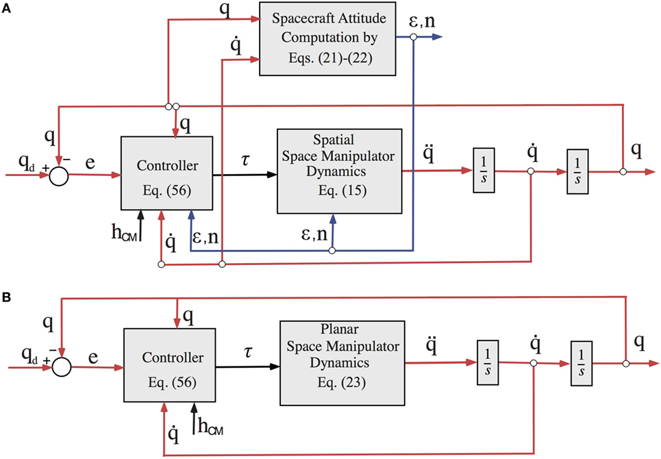
Figure 2. (A) The PD control with angular momentum compensation (PDC-AMC) applied on a spatial free-floating space manipulator system (FFSMS). The computed spacecraft attitude should be also used as feedback. (B) The PDC-AMC applied on a planar FFSMS. Only the joint angles and rates are used as feedback.

However, the application of the PDC-AMC on planar FFSMS requires only the measurement and the feedback of the joint angles q and the joint rates $\dot{\mathbf{\text{q}}}$, see Figure 2B.

Due to the presence of angular momentum on the FFSMS, to maintain the manipulator joints at the desired angles at steady state, the controller must apply time-varying joint torques,

$\mathbf{\text{τ}}={\mathbf{\text{g}}}_{\mathbf{\text{h}}}\left({\mathbf{\text{h}}}_{\mathbf{\text{cm}}},\mathbf{\text{ε}},n,{\mathbf{\text{q}}}_{\mathbf{\text{ss}}}\right)$ (65)

These torques, in case of planar FFSMS are constant, since they are independent from the spacecraft attitude:

$\mathbf{\text{τ}}={\mathbf{\text{g}}}_{\mathbf{\text{h}}}\left(h_{\mathit{CM}},{\mathbf{\text{q}}}_{\mathbf{\text{ss}}}\right)$ (66)

Tracking Control

We study tasks where, instead of point-to-point motions, the tracking of a desired joint trajectory is required. The desired joint trajectory is described by the functions q_d(t), ${\dot{\mathbf{\text{q}}}}_{\mathbf{\text{d}}}\left(t\right)$, and ${\ddot{\mathbf{\text{q}}}}_{\mathbf{\text{d}}}\left(t\right)$. The application of the following model-based controller, which contains both the terms C*, g_h, caused by the angular momentum, on the system equations of motion, see Eq. 15.

$\mathbf{\text{τ}}=\mathbf{\text{H}}\left(\mathbf{\text{q}}\right)\left({\ddot{\mathbf{\text{q}}}}_{\mathbf{\text{d}}}+{\mathbf{\text{K}}}_{\mathbf{\text{p}}}\left({\mathbf{\text{q}}}_{\mathbf{\text{d}}}-\mathbf{\text{q}}\right)+{\mathbf{\text{K}}}_{\mathbf{\text{d}}}\left({\dot{\mathbf{\text{q}}}}_{\mathbf{\text{d}}}-\dot{\mathbf{\text{q}}}\right)\right)+{\mathbf{\text{C}}}^{\ast }\dot{\mathbf{\text{q}}}+{\mathbf{\text{g}}}_{\mathbf{\text{h}}}$ (67)

results in the following error dynamics:

$\ddot{\mathbf{\text{e}}}+{\mathbf{\text{K}}}_{\mathbf{\text{d}}}\dot{\mathbf{\text{e}}}+{\mathbf{\text{K}}}_{\mathbf{\text{p}}}\mathbf{\text{e}}=\mathbf{0}$ (68)

where the selection of appropriate positive definite gain matrices K_p, K_d ensures the stability of the dynamics and zero steady state joint error in desired time.

The abovementioned controller uses all the system dynamics (i.e., the terms H, C*, and g_h) so that the joint errors will be 0 after desired time. However, the full implementation of Eq. 67 may be constrained by the available computing power in space that in general lags the one on earth. As an alternative, we propose the use of the PDC-AMC, which requires the feedback of only a part of the system dynamics, i.e., the term g_h given by Eqs 18 and 25 for spatial and planar FFSMS, respectively, with appropriate PD gains. In this case, the error dynamics is given by:

$\mathbf{\text{H}}\ddot{\mathbf{\text{e}}}+\left({\mathbf{\text{C}}}^{\ast }+{\mathbf{\text{K}}}_{\mathbf{\text{d}}}\right)\dot{\mathbf{\text{e}}}+{\mathbf{\text{K}}}_{\mathbf{\text{p}}}\mathbf{\text{e}}=\mathbf{\text{H}}{\ddot{\mathbf{\text{q}}}}_{\mathbf{\text{d}}}+\left({\mathbf{\text{C}}}^{\ast }+{\mathbf{\text{K}}}_{\mathbf{\text{d}}}\right){\dot{\mathbf{\text{q}}}}_{\mathbf{\text{d}}}$ (69)

The stability of PD with gravity compensation controller for trajectory tracking problems and fixed base manipulators has been studied in Wang et al. (1996) and Wen and Kreutz-Delgado (1992). It has been shown that the position tracking error converges to a closed ball, which size can be arbitrary small by increasing the controller gains. Since fixed base manipulators and FFSMS with NZAM exhibit the same properties of the dynamic model (Eq. 34), the analysis proposed in Wang et al. (1996) and Wen and Kreutz-Delgado (1992) can be extended to the stability of the PDC-AMC in trajectory tracking applications. Note that, increasing the gains, the torques become smaller due to the fact that larger gains give “tighter” performance, and hence smaller tracking errors (Lewis et al., 2004). However, due to the presence of signal noise, the use of large gains is limited in practice since it may result in poor response. Therefore, gains must be selected accordingly.

Control in the Cartesian Space

Many tasks required in on-orbit servicing activities are carried out in the Cartesian space where the end-effector is driven to a desired location ${\mathbf{\text{x}}}_{\mathbf{\text{E,d}}}=[\begin{array}{cc}\hfill {\mathbf{\text{r}}}_{\mathbf{\text{E}},\mathbf{\text{d}}}^{\text{T}}\hfill & \hfill {\mathbf{\text{θ}}}_{\mathbf{\text{E}},\mathbf{\text{d}}}^{\text{T}}]\hfill \end{array}$ (point-to-point control) or it is commanded to follow a Cartesian trajectory ${\mathbf{\text{x}}}_{\mathbf{\text{E,d}}}\left(t\right)=[\begin{array}{cc}\hfill {\mathbf{\text{r}}}_{\mathbf{\text{E}},\mathbf{\text{d}}}^{\text{T}}\left(t\right)\hfill & \hfill {\mathbf{\text{θ}}}_{\mathbf{\text{E}},\mathbf{\text{d}}}^{\text{T}}\left(t\right)\hfill \end{array}]$ (tracking control), where r_E,d and θ_E,d are the desired end-effector position and the desired end-effector attitude expressed by the Euler angles, respectively.

Point-to-Point Control

In the case of FFSMS with zero angular momentum and considering invertible GJM, the point-to-point control can be achieved by a control law of the form (Papadopoulos and Dubowsky, 1991b):

$\mathbf{\text{τ}}={\mathbf{\text{J}}}_{\mathbf{\text{q}}}^{\text{T}}\left({\mathbf{\text{K}}}_{\mathbf{\text{p}}}{\mathbf{\text{e}}}_{\mathbf{\text{x}}}-{\mathbf{\text{K}}}_{\mathbf{\text{d}}}{\mathbf{\text{v}}}_{\mathbf{\text{E}}}\right)$ (70)

where K_p, K_d are the gain matrices of the controller and e_x is the Cartesian error:

${\mathbf{\text{e}}}_{\mathbf{\text{x}}}=\left[\begin{array}{c}\hfill {\mathbf{\text{r}}}_{\mathbf{\text{E}},\mathbf{\text{d}}}\hfill \\ \hfill {\mathbf{\text{θ}}}_{\mathbf{\text{E}},\mathbf{\text{d}}}\hfill \end{array}\right]-\left[\begin{array}{c}\hfill {\mathbf{\text{r}}}_{\mathbf{\text{E}}}\hfill \\ \hfill {\mathbf{\text{θ}}}_{\mathbf{\text{E}}}\hfill \end{array}\right]$ (71)

However, considering an invertible GJM and a desired end-effector set-point $\left({\dot{\mathbf{\text{v}}}}_{\mathbf{\text{E,d}}}={\mathbf{\text{v}}}_{\mathbf{\text{E,d}}}=\mathbf{0}\right)$, the application of the above controller to an FFSMS with NZAM results in the following error dynamics for a planar and a spatial FFSMS, respectively:

${\mathbf{\text{H}}}_{\mathbf{\text{x}}}{\ddot{\mathbf{\text{e}}}}_{\mathbf{\text{x}}}+\left({\mathbf{\text{C}}}_{\mathbf{\text{x}}}^{\ast }+{\mathbf{\text{J}}}_{\mathbf{\text{q}}}^{\text{T}}{\mathbf{\text{K}}}_{\mathbf{\text{d}}}\right){\dot{\mathbf{\text{e}}}}_{\mathbf{\text{x}}}+{\mathbf{\text{J}}}_{\mathbf{\text{q}}}^{\text{T}}{\mathbf{\text{K}}}_{\mathbf{\text{p}}}{\mathbf{\text{e}}}_{\mathbf{\text{x}}}={\mathbf{\text{g}}}_{\mathbf{\text{x}}}\left({\mathrm{\theta }}_0,\mathbf{\text{q}},\dot{\mathbf{\text{q}}},h_{\mathit{CM}}\right)$ (72)

and

${\mathbf{\text{H}}}_{\mathbf{\text{x}}}{\ddot{\mathbf{\text{e}}}}_{\mathbf{\text{x}}}+\left({\mathbf{\text{C}}}_{\mathbf{\text{x}}}^{\ast }+{\mathbf{\text{J}}}_{\mathbf{\text{q}}}^{\text{T}}{\mathbf{\text{K}}}_{\mathbf{\text{d}}}\right){\dot{\mathbf{\text{e}}}}_{\mathbf{\text{x}}}+{\mathbf{\text{J}}}_{\mathbf{\text{q}}}^{\text{T}}{\mathbf{\text{K}}}_{\mathbf{\text{p}}}{\mathbf{\text{e}}}_{\mathbf{\text{x}}}={\mathbf{\text{g}}}_{\mathbf{\text{x}}}\left(\mathbf{\text{ε}},n,\mathbf{\text{q}},\dot{\mathbf{\text{q}}},{\mathbf{\text{h}}}_{\mathbf{\text{CM}}}\right)$ (73)

For NZAM, the term g_x is non-zero. Therefore, both Eqs 72 and 73 will result in a time varying Cartesian error e_x that can be reduced by increasing the control gains, but cannot be eliminated. This is due to the fact that Eq. 70 is of PD type and g_x is a non-zero system disturbance. Similar to the case of joint control, the nature of the time-varying errors can be explained considering that the time-varying joint torques required to compensate the time-varying centrifugal torques can only be developed by a time-varying non-zero error, according to Eq. 70. Therefore, the above controller is not suitable for eliminating errors in the presence of NZAM.

Next, we study set point and tracking Cartesian space controllers for eliminating the corresponding end-effector errors in the presence of angular momentum.

First, the design of a control law tackling the point-to-point control problem, under the presence of angular momentum, is studied. This controller is called here transposed Jacobian control with angular momentum compensation (TJC-AMC) (Nanos, 2015).

Exploiting the dynamic model, given by Eq. 28, a control law is developed to drive the end-effector to a desired Cartesian point despite the NZAM. The following Lyapunov function is selected so that the control law u to be developed ensures the end-effector asymptotic stability (Nanos, 2015):

$V\left({\mathbf{\text{v}}}_{\mathbf{\text{E}}},{\mathbf{\text{e}}}_{\mathbf{\text{x}}}\right)=\frac{1}{2}{\mathbf{\text{v}}}_{\mathbf{\text{E}}}^{\text{T}}{\mathbf{\text{H}}}_{\mathbf{\text{x}}}{\mathbf{\text{v}}}_{\mathbf{\text{E}}}+\frac{1}{2}{\mathbf{\text{e}}}_{\mathbf{\text{x}}}^{\mathbf{\text{T}}}{\mathbf{\text{K}}}_{\mathbf{\text{p}}}{\mathbf{\text{e}}}_{\mathbf{\text{x}}}$ (74)

The inertia matrix H_x is positive definite iff the matrix J_q is invertible. In this case, if one selects a positive definite matrix K_p, the following is true:

$V\left({\mathbf{\text{v}}}_{\mathbf{\text{E}}},{\mathbf{\text{e}}}_{\mathbf{\text{x}}}\right)>0$ (75)

and

$V\left(\mathbf{0},\mathbf{0}\right)=0$ (76)

The time derivative of the Lyapunov function is:

$\dot{V}\left({\mathbf{\text{v}}}_{\mathbf{\text{E}}},{\mathbf{\text{e}}}_{\mathbf{\text{x}}}\right)=\frac{1}{2}{\mathbf{\text{v}}}_{\mathbf{\text{E}}}^{\text{T}}{\dot{\mathbf{\text{H}}}}_{\mathbf{\text{x}}}{\mathbf{\text{v}}}_{\mathbf{\text{E}}}+{\mathbf{\text{v}}}_{\mathbf{\text{E}}}^{\text{T}}{\mathbf{\text{H}}}_{\mathbf{\text{x}}}{\dot{\mathbf{\text{v}}}}_{\mathbf{\text{E}}}+{\mathbf{\text{e}}}_{\mathbf{\text{x}}}^{\text{T}}{\mathbf{\text{K}}}_{\mathbf{\text{p}}}{\dot{\mathbf{\text{e}}}}_{\mathbf{\text{x}}}$ (77)

where the term ${\mathbf{\text{H}}}_{\mathbf{\text{x}}}{\dot{\mathbf{\text{v}}}}_{\mathbf{\text{E}}}$ can be substituted using Eq. 28 resulting in:

$\dot{V}\left({\mathbf{\text{v}}}_{\mathbf{\text{E}}},{\mathbf{\text{e}}}_{\mathbf{\text{x}}}\right)={\mathbf{\text{v}}}_{\mathbf{\text{E}}}^{\text{T}}\left(\mathbf{\text{u}}-{\mathbf{\text{g}}}_{\mathbf{\text{x}}}-{\mathbf{\text{K}}}_{\mathbf{\text{p}}}{\mathbf{\text{e}}}_{\mathbf{\text{x}}}\right)+\frac{1}{2}{\mathbf{\text{v}}}_{\mathbf{\text{E}}}^{\text{T}}\left({\dot{\mathbf{\text{H}}}}_{\mathbf{\text{x}}}-2{\mathbf{\text{C}}}_{\mathbf{\text{x}}}^{\ast }\right){\mathbf{\text{v}}}_{\mathbf{\text{E}}}$ (78)

where we considered that ${\dot{\mathbf{\text{e}}}}_{\mathbf{\text{x}}}=-{\mathbf{\text{v}}}_{\mathbf{\text{E}}}$, since x_E,d = const, and K_p is symmetric $\left({\mathbf{\text{K}}}_{\mathbf{\text{p}}}={\mathbf{\text{K}}}_{\mathbf{\text{p}}}^{\text{T}}\right)$.

As shown in Section “Dynamics of Free-Floating Space Manipulators,” see Eq. 40, the second term of the RHS of the Eq. 78 is 0. Therefore, the selection of the following input:

$\mathbf{\text{u}}={\mathbf{\text{K}}}_{\mathbf{\text{p}}}{\mathbf{\text{e}}}_{\mathbf{\text{x}}}-{\mathbf{\text{K}}}_{\mathbf{\text{d}}}{\mathbf{\text{v}}}_{\mathbf{\text{E}}}+{\mathbf{\text{g}}}_{\mathbf{\text{x}}}$ (79)

with positive definite gain matrix K_d, results in:

$\dot{V}\left({\mathbf{\text{v}}}_{\mathbf{\text{E}}},{\mathbf{\text{e}}}_{\mathbf{\text{x}}}\right)=-{\mathbf{\text{v}}}_{\mathbf{\text{E}}}^{\text{T}}{\mathbf{\text{K}}}_{\mathbf{\text{d}}}{\mathbf{\text{v}}}_{\mathbf{\text{E}}}\le 0$ (80)

Equation 80 does not guarantee the asymptotic stability of the origin (v_E, e_x) = (0,0), since $\dot{V}$ = 0 only when v_E = 0 regardless the joint error e. Then, we show that $\dot{V}$ = 0 only when v_E = 0 and e_x = 0. Suppose that the end-effector stops $\left({\mathbf{\text{v}}}_{\mathbf{\text{E}}}=\mathbf{0},{\dot{\mathbf{\text{v}}}}_{\mathbf{\text{E}}}=\mathbf{0}\right)$ at a manipulator configuration where e_x ≠ 0. Applying the control law, given by Eq. 79, in Eq. 28 and considering that v_E = 0 [e.g., ($\dot{V}$ = 0)], results in:

${\dot{\mathbf{\text{v}}}}_{\mathbf{\text{E}}}={\mathbf{\text{H}}}_{\mathbf{\text{x}}}^{-1}{\mathbf{\text{K}}}_{\mathbf{\text{p}}}{\mathbf{\text{e}}}_{\mathbf{\text{x}}}$ (81)

When GJM is invertible, the matrices H_x and K_p are positive definite, and Eq. 81 results in ${\dot{\mathbf{\text{v}}}}_{\mathbf{\text{E}}}\ne \mathbf{0}$ when e_x ≠ 0. Therefore, the end-effector stops only when e_x = 0. Thus, $\dot{V}$ = 0 only when v_E = 0 and e_x = 0, and according to the La Salle theorem, the origin (v_E, e_x) = (0,0) is asymptotically stable.

Therefore, using Eqs 29 and 79, the required joint torques are obtained by TJC-AMC (Nanos, 2015):

$\mathbf{\text{τ}}={\mathbf{\text{J}}}_{\mathbf{\text{q}}}^{\text{T}}\left({\mathbf{\text{K}}}_{\mathbf{\text{p}}}{\mathbf{\text{e}}}_{\mathbf{\text{x}}}-{\mathbf{\text{K}}}_{\mathbf{\text{d}}}{\mathbf{\text{v}}}_{\mathbf{\text{E}}}\right)+{\mathbf{\text{J}}}_{\mathbf{\text{q}}}^{\text{T}}{\mathbf{\text{g}}}_{\mathbf{\text{x}}}$ (82)

The gain matrices K_p, K_d of the controller can be chosen as diagonal matrices with diagonal elements given by Eqs 57 and 58 considering now as h_ii the diagonal element of the matrix H_x.

Since the angular momentum of the FFSMS is non-zero, to maintain the end-effector at the desired location, the controller must apply non-zero joint torques,

$\mathbf{\text{τ}}={\mathbf{\text{g}}}_{\mathbf{\text{h}}}\left(\mathbf{\text{ε}},n,\mathbf{\text{q}},{\mathbf{\text{h}}}_{\mathbf{\text{CM}}}\right)$ (83)

Note that in the case of zero initial angular momentum, the term g_x vanishes and the controller given by Eq. 82 takes the controller’s form given by Eq. 70.

Tracking Control

Similar to the case of joint space control, to track a desired end-effector trajectory described by the functions x_E,d(t), v_E,d(t), and ${\dot{\mathbf{\text{v}}}}_{\mathbf{\text{E,d}}}\left(t\right)$, the application of the following model-based controller:

$\mathbf{\text{τ}}={\mathbf{\text{J}}}_{\mathbf{\text{q}}}^{\text{T}}\left({\mathbf{\text{H}}}_{\mathbf{\text{x}}}\left({\dot{\mathbf{\text{v}}}}_{\mathbf{\text{E,d}}}+{\mathbf{\text{K}}}_{\mathbf{\text{d}}}{\dot{\mathbf{\text{e}}}}_{\mathbf{\text{x}}}+{\mathbf{\text{K}}}_{\mathbf{\text{p}}}{\mathbf{\text{e}}}_{\mathbf{\text{x}}}\right)+{\mathbf{\text{C}}}_{\mathbf{\text{x}}}^{\ast }{\mathbf{\text{v}}}_{\mathbf{\text{E}}}+{\mathbf{\text{g}}}_{\mathbf{\text{x}}}\right)$ (84)

results in the following error dynamics:

${\ddot{\mathbf{\text{e}}}}_{\mathbf{\text{x}}}+{\mathbf{\text{K}}}_{\mathbf{\text{d}}}{\dot{\mathbf{\text{e}}}}_{\mathbf{\text{x}}}+{\mathbf{\text{K}}}_{\mathbf{\text{p}}}{\mathbf{\text{e}}}_{\mathbf{\text{x}}}=\mathbf{0}$ (85)

where the selection of appropriate positive definite gain matrices K_p, K_d ensures the stability of the dynamics and zero steady state Cartesian error in desired time.

As explained earlier, in the case of limited computing power, this control law can be substituted by the TJC-AMC given by Eq. 82, as it requires less computations, with the drawback of higher gains. In this case, the error dynamics is given by:

${\mathbf{\text{H}}}_{\mathbf{\text{x}}}{\ddot{\mathbf{\text{e}}}}_{\mathbf{\text{x}}}+\left({\mathbf{\text{C}}}_{\mathbf{\text{x}}}^{\ast }+{\mathbf{\text{K}}}_{\mathbf{\text{d}}}\right){\dot{\mathbf{\text{e}}}}_{\mathbf{\text{x}}}+{\mathbf{\text{K}}}_{\mathbf{\text{p}}}{\mathbf{\text{e}}}_{\mathbf{\text{x}}}={\mathbf{\text{H}}}_{\mathbf{\text{x}}}{\dot{\mathbf{\text{v}}}}_{\mathbf{\text{E,d}}}+\left({\mathbf{\text{C}}}_{\mathbf{\text{x}}}^{\ast }+{\mathbf{\text{K}}}_{\mathbf{\text{d}}}\right){\mathbf{\text{v}}}_{\mathbf{\text{E,d}}}$ (86)

The stability of the TJC-AMC with large gains can be shown with a similar analysis proposed in Wang et al. (1996) and Wen and Kreutz-Delgado (1992), since, as have been shown, the same properties of dynamic model are valid both for fixed base manipulators and FFSMS with NZAM.

Note that the development of the proposed controllers (i.e., PDC-AMC and TJC-AMC) assumes the exact knowledge of the system kinematic and inertial parameters. Similar to the fixed base manipulators, the presence of dynamic uncertainties results in additional non-zero terms in the RHS of the error dynamics, given by Eqs 69 and 86. The presence of these terms causes undesirable non-zero errors. However, their effect decreases as the controller gains become higher, see Wang et al. (1996).

Constraints

To compensate the effect of NZAM, the application of controllers similar to ones used for compensation of gravity in the terrestrial fixed base manipulators is proposed. In contrast to fixed base manipulators and as shown in Section “Control in the Presence of Angular Momentum,” the implementation of these controllers requires also the knowledge of spacecraft attitude.

Moreover, since the use of these control laws, in the Cartesian space, requires the use of the transpose and the inverse of the GJM, this matrix must be invertible during the motion of the end-effector so that no DS are encountered (Papadopoulos and Dubowsky, 1993). It is known that a DS may occur when the end-effector is in the path-dependent workspace (PDW) area (Papadopoulos and Dubowsky, 1993). As shown in Figure 3A, in this area, the end-effector velocities ${\dot{\mathbf{\text{r}}}}_{\mathbf{\text{E,1}}},{\dot{\mathbf{\text{r}}}}_{\mathbf{\text{E,2}}}$ caused by the joint rates $\dot{\mathbf{\text{q}}}=[\begin{array}{cc}\hfill {\dot{q}}_1\hfill & \hfill 0\hfill \end{array}]$ and $\dot{\mathbf{\text{q}}}=[\begin{array}{cc}\hfill 0\hfill & \hfill {\dot{q}}_2\hfill \end{array}]$, respectively, and the base reaction may have the same direction. In this case, the end-effector velocity ${\dot{\mathbf{\text{r}}}}_{\mathbf{\text{E}}}$, as the vector sum of these velocities, will have the same direction regardless the joint rates and the end-effector can move only along this direction. However, if the end-effector is in the path-independent workspace (PIW) area, Figure 3B, the velocity ${\dot{\mathbf{\text{r}}}}_{\mathbf{\text{E}}}$ can have any desired direction, depending on the joint rates, and no DS occur. Thus, to avoid any failure of the TJC-AMC, the end-effector must be in the PIW during its motion. Else, the initial spacecraft attitude and manipulator configuration should be selected to avoid DS (Nanos and Papadopoulos, 2015). The abovementioned constraints must be considered regardless of the existence of NZAM (Papadopoulos and Dubowsky, 1991a). However, the initial configuration range, required to avoid a DS, depends on the amount of the accumulated angular momentum.

FIGURE 3

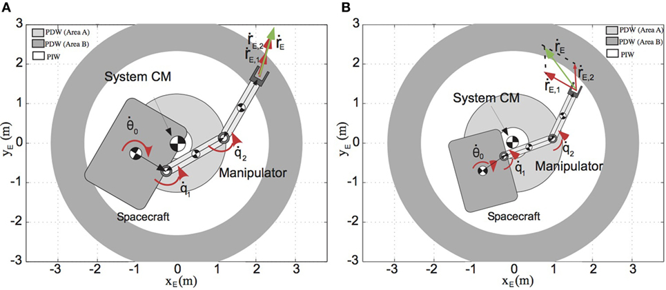
Figure 3. (A) The location of the end-effector at the path-dependent workspace (PDW) area may result in dynamic singularities (DS). (B) The end-effector location at the path-independent workspace (PIW) results in DS avoidance.

The presence of NZAM imposes an additional constraint. It is well known that in the absence of angular momentum, the end-effector can remain fixed at a point of the reachable workspace, since, in this case, all the system configuration variables remain fixed, too. However, the existence of angular momentum results to a system’s motion according to the conservation of the angular momentum. This may result in DS and cause the end-effector to be displaced from its desired location. It can be shown that the workspace area, where the end-effector can remain indefinitely executing a task under the presence of NZAM is the same with the PIW area. This observation results from the kinematic and dynamic constraints of the system (Nanos and Papadopoulos, 2011). Thus, to avoid any possible failure of the TJC-AMC, the initial and the final desired location of the end-effector must be in the PIW area.

Discussion

The above analysis showed that in the case of the control of FFSMS with NZAM, the application of controllers, which ignore the system initial angular momentum (e.g., PD control law) results in final non-zero errors both in joint and Cartesian space. In this paper, we exploited the dynamics of FFSMS with NZAM in order to design controllers, which tackle this problem. In the joint space, the proposed PDC-AMC can drive the system manipulator configuration to the desired one despite the presence of NZAM. For applications in the Cartesian space, the TJC-AMC is proposed in order to drive the end-effector to a desired location without drift it away contrary to other control laws (Matsuno and Saito, 2001). In the next section, these results are illustrated by examples.

Examples

Example 1

To illustrate the PDC-AMC, given by Eq. 56, first the planar FFSMS in Figure 4 with parameters in Table 1 is employed. The initial angular momentum of the robot is h_CM = 15 Nm s. It is desired to drive the manipulator from the initial configuration (q_1,in, q_2,in) = (10°, 20°) to the desired final configuration (q_1,fin, q_2,fin) = (50°, 100°).

FIGURE 4

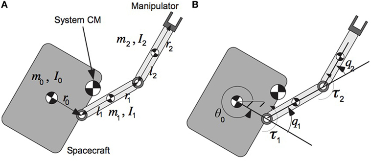
Figure 4. A planar free-floating space manipulator system with two revolute joints. (A) Definition of the inertia parameters and (B) definition of the system variables.

TABLE 1

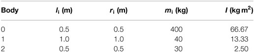
Table 1. Parameters of the system shown in Figure 4.

First, the PD controller, given by Eq. 45, which does not take into account the presence of the initial angular momentum of the FFSMS, is applied to the system. The controller gains are selected using the Eqs 57 and 58 and they are equal to K_p = diag(17.9, 2.3) and K_d = diag(59.7, 7.6). We assume that the spacecraft attitude at the moment where the control input is applied, is θ_0,in = 0°. As shown in Figure 5A, the joint angles are not driven to the desired values since q_1,ss = 49.67° and q_2,ss = 97.83°. A constant steady-state error exists. This error becomes more evident when the system accumulated angular momentum is increased or when the manipulator inertia parameters are comparable with the ones of the spacecraft (e.g., during a capturing operation). To tackle this problem, the PDC-AMC with the same gains is applied, next. Figure 5C shows the response of the joint angles. It is shown that the desired joint angles are achieved. The torques applied on the joints for both controllers are shown in Figures 5B,D. Due to the NZAM, non-zero torques are required (i.e., τ_1,ss = 0.105 Nm and τ_2,ss = 0.0866 Nm) so that the manipulator maintains at the final configuration. Figure 6 shows snapshots of the resulting motion of the system. Due to the NZAM, the spacecraft attitude continues to change.

FIGURE 5

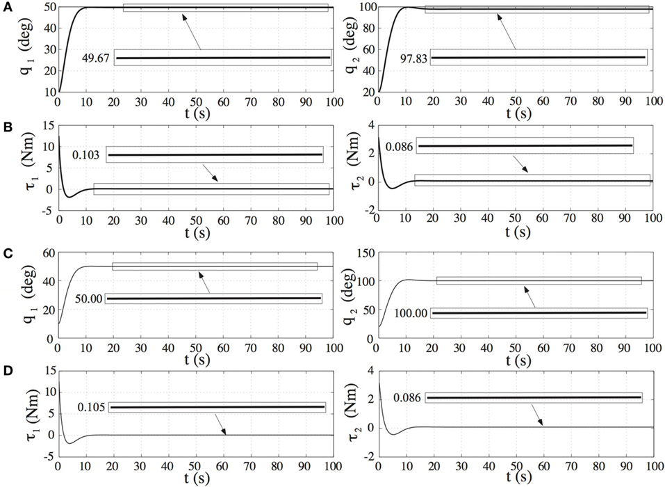
Figure 5. (A) The response of the manipulator configuration, (B) the required joint torques caused by the application of the PD control law, given by Eq. 45, on the planar free-floating space manipulator systems (FFSMS) shown in Figure 4, (C) the response of the manipulator configuration, (D) the required joint torques result by the application of the PD control with angular momentum compensation on the planar FFSMS shown in Figure 4.

FIGURE 6

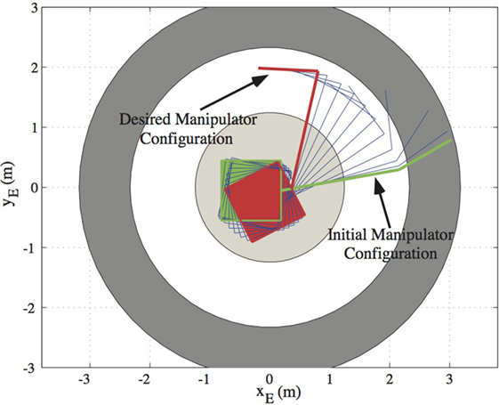
Figure 6. The motion of the planar free-floating space manipulator system results from the implementation of the PD control with angular momentum compensation.

Next, the spatial FFSMS shown in Figure 1 with parameters in Table 2 is employed. The initial angular momentum of the robot is h_CM = [68 66 65]^T Nm s. It is desired to drive the system manipulator from the initial configuration q_in = [10°30°40°]^T to the final desired configuration q_fin = [60°70°90°]^T. At the time of the controller application, the spacecraft attitude is given by the initial Euler parameters ${\left[\begin{array}{cc}\hfill {\mathbf{\text{ε}}}_{\mathbf{\text{in}}}^{\text{T}}\hfill & \hfill n\hfill \end{array}\right]}^{\text{T}}=[{\begin{array}{cccc}\hfill 0.1\hfill & \hfill 0.5\hfill & \hfill 0.3\hfill & \hfill 0.8062\hfill \end{array}]}^{\text{T}}$.

TABLE 2

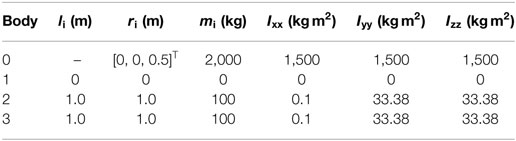
Table 2. Parameters of the system shown in Figure 1.

The control law given by Eq. 45 is applied first. The controller gains are diagonal matrices with elements obtained by Eqs 57 and 58 and given by K_p = diag(63.7, 187.1, 31.9) and K_d = diag(212.3, 623.5, 106.2). The implementation of this controller results in time-varying final errors in manipulator configuration, as shown in Figure 7A. Figure 7B shows the required torques applied by the controller.

FIGURE 7

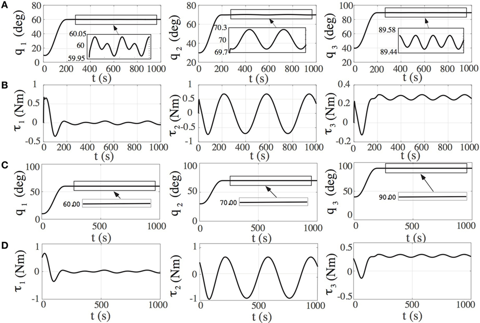
Figure 7. (A) The response of the manipulator configuration, (B) the required joint torques result by the application of the PD control law, given by Eq. 45, on the spatial free-floating space manipulator system (FFSMS) shown in Figure 1, (C) the response of the manipulator configuration, (D) the required joint torques result by the application of the PD control with angular momentum compensation on the spatial FFSMS shown in Figure 1.

Next, the application of the PDC-AMC, with the same gains, is proposed. As shown in Figure 7C, the PDC-AMC drives the manipulator to the desired configuration with zero steady-state errors. Due to the NZAM, time-varying torques required at the steady state in order to maintain the desired configuration, see Figure 7D.

Example 2

In this example, the TJC-AMC, given by Eq. 82, is applied to the planar space manipulator system in Figure 4 with parameters in Table 1. The initial angular momentum of the robot is h_CM = 15 Nm s. It is desired to drive the end-effector from point A(1.0, 1.5) m to points B(−0.8, 1.8) m or C (−2.0, 2.0) m despite the presence of NZAM.

To demonstrate the problem of ignoring the system angular momentum, the control law, given by Eq. 70, is applied first. The controller gains are selected applying Eqs 57 and 58, considering this time as h_ii the diagonal elements of the matrix H_x, and they are equal to K_p = diag(16.1, 368.1) and K_d = diag(80.5, 1,840.7). We assume that the spacecraft attitude at the moment where the control input is applied, is θ_0,in = 60°. In this case, the manipulator configuration, which corresponds to the initial point A(1.0, 1.5) m is q₁ = − 37.3° and q₂ = 130.2°. It is desired to drive the end-effector to point B(−0.8, 1.8) m. To avoid the application of large required torques at the beginning of the motion, a trapezoid velocity profile is applied as a reference input in the closed-loop system. Figure 8A shows the response of the end-effector position. It is shown that the system angular momentum results in a time-varying final error in end-effector position. The required torques are shown in Figure 8B.

FIGURE 8

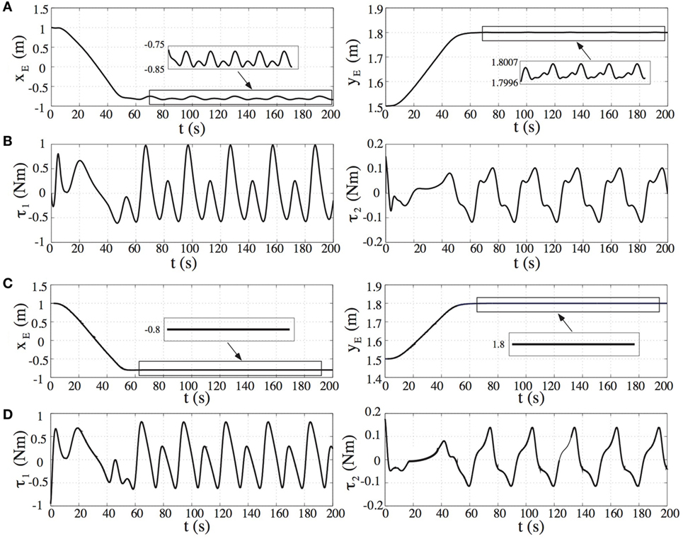
Figure 8. (A) The end-effector position and (B) the required joint torques result by the application of the transpose Jacobian controller, given by Eq. 70, (C) the end-effector position, and (D) the required joint torques result by the application of the transposed Jacobian control with angular momentum compensation.

Next, the TJC-AMC with the same control gains is applied. As shown in Figure 8C, the end-effector arrives at the desired final position with zero steady-state errors despite the NZAM. However, due to this, non-zero torques are required so that the end-effector stays at the desired position. The torques applied on the joints are shown in Figure 8D. Figure 9 shows snapshots of the resulting motion of the system.

FIGURE 9

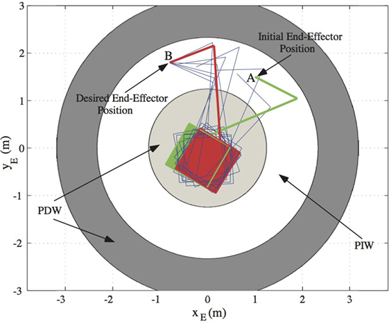
Figure 9. The motion of the space manipulator results from a successful application of the transposed Jacobian control with angular momentum compensation. The end-effector path lies in the path-independent workspace (PIW) area.

Next, the case where the end-effector is driven to point C in the PDW area is studied; see Figure 10. As mentioned in Section “Discussion,” DS avoidance, which results in a successful end-effector approach to point C, depends on the initial spacecraft attitude. A method to compute the appropriate initial spacecraft attitudes to avoid a DS can be found in Nanos and Papadopoulos (2015). In case the spacecraft initial attitude is θ_0,in = 270°, the controller fails at point D, see Figure 10A. In the neighborhood of the singular point D, the determinant of GJM is closed to 0 resulting in too large required joint torques even for small end-effector displacements, as shown in Figure 11.

FIGURE 10

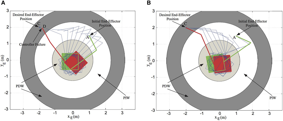
Figure 10. (A) The motion of the space manipulator results from a failed application of the transposed Jacobian control with angular momentum compensation (TJC-AMC). At the point D of the path-dependent workspace (PDW) area, the manipulator becomes singular. (B) The motion of the space manipulator results from a successful application of the TJC-AMC.

FIGURE 11

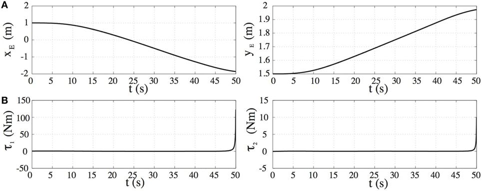
Figure 11. (A) The trajectories of the end-effector position, and (B) the required joint torques for the FFSM motion shown in Figure 10A.

Then, the case of spacecraft initial attitude equal to θ_0,in = 10° is examined. In this case, the TJC-AMC drives the end-effector to the desired point C. Figure 10B shows the snapshots of the motion and Figures 12A,B the end-effector trajectory and the joint torques. The end-effector remains fixed, at point C while both manipulator and spacecraft move due to the NZAM. However, since point C belongs to the PDW area, the manipulator may become singular later in time resulting in a failure of the TJC-AMC, see Figures 12C,D.

FIGURE 12

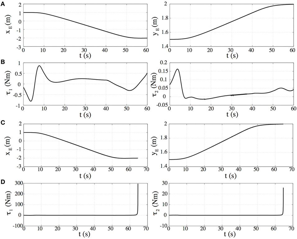
Figure 12. (A) The trajectories of the end-effector position, and (B) the required joint torques for the FFSM motion shown in Figure 10B. (C) The trajectories of the end-effector position, and (D) the required joint torques for the FFSM motion shown in Figure 10B including the time where the end-effector position maintains at point C. Notice the difference in the time axes between panels (A,B) and (C,D).

Example 3

Here, the TJC-AMC, given by Eq. 82, is applied to trajectory tracking applications both for planar and spatial FFSMS. First, the end-effector of the planar FFSMS, shown in Figure 4 with parameters in Table 1, is desired to follow a straight line path from point A(1.5, 0.0) m to point B(−0.8, 1.8) m in time t_f = 100 s. The initial angular momentum of the system is h_CM = 15 Nm s.

As mentioned above, in order to achieve trajectory tracking, high controller gains are required. These gains are selected, using Eqs 57 and 58 and considering that the closed loop frequency must be bigger that the frequency of the desired trajectory. In this application, the controller gains are selected equal to K_p = diag(1,285, 81,203) and K_d = diag(257, 16,241). The desired end-effector path crosses the PDW area and, therefore, a DS may appear during its motion. However, since the end-effector desired trajectory is given, one can exploit the methodology presented in Nanos and Papadopoulos (2015) to find the initial spacecraft attitude in order to avoid any possible DS. Applying this method, one can find that an initial feasible spacecraft attitude is θ_0,in = 200°. The desired trajectory is given by:

$y_E\left(t\right)=K{x}_E\left(t\right)+L$ (87)

where one can set

$x_E\left(t\right)=x_{\text{in}}+\left(x_{\text{fin}}-x_{\text{in}}\right)s\left(t\right)$ (88)

where x_in, x_fin correspond to the initial and final position of the end-effector and s(t) is the arc length parameterization of the path, given by:

$s\left(t\right)=a_0+a_{1}t+a_2{t}^2+a_3{t}^3+a_4{t}^4+a_5{t}^5,0\le t\le t_{\text{fin}}$ (89)

with s(0) = 0, $s\left(t_{\text{fin}}\right)=1$, and $\dot{s}\left(0\right)=\ddot{s}\left(0\right)=\dot{s}\left(t_f\right)=\ddot{s}\left(t_f\right)=0$.

Figure 13A shows the response of the end-effector position compared with the desired end-effector trajectories and snapshots of corresponding motion the planar FFSMS. It is shown that the end-effector follows the desired path. Figure 13A shows also the torques required for this end-effector motion.

FIGURE 13

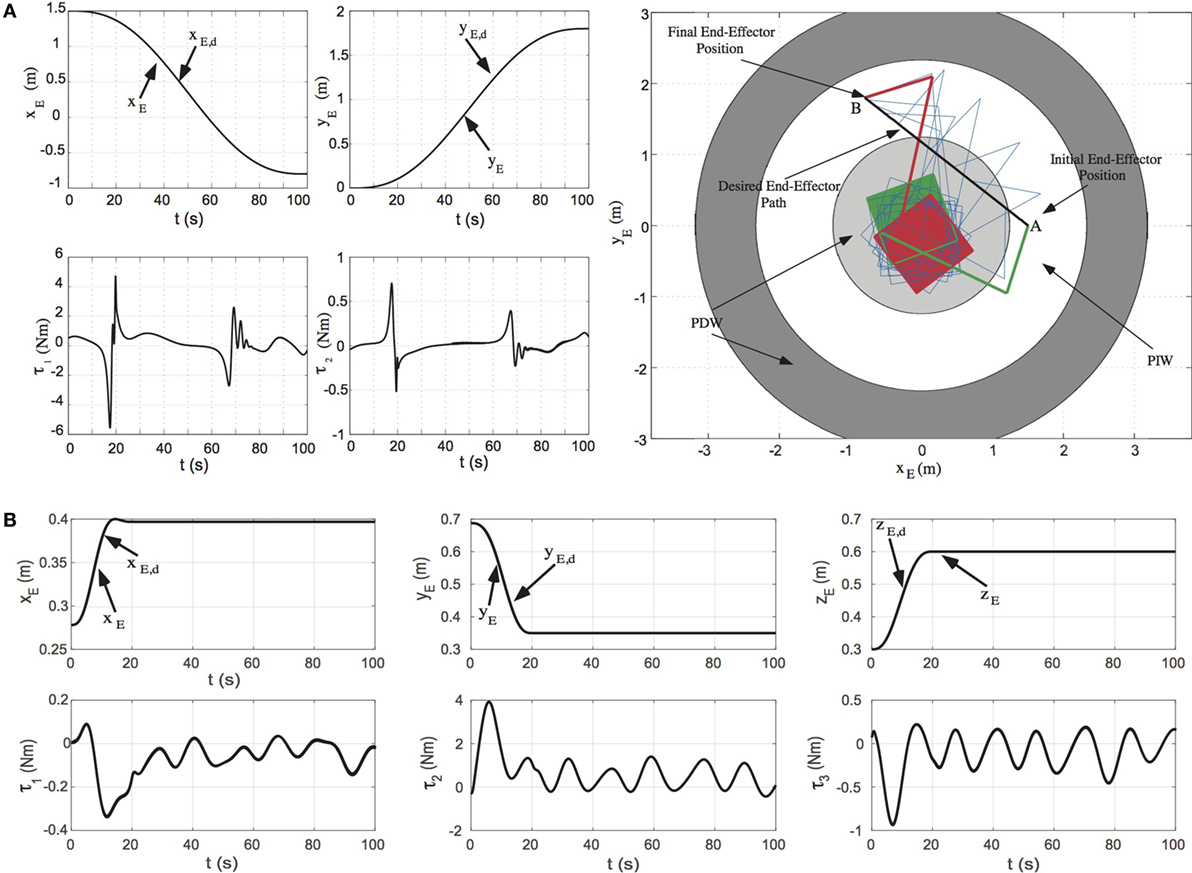
Figure 13. (A) Planar free-floating space manipulator systems (FFSMS): the trajectories of the end-effector position compared with the desired ones, the required joint torques, and snapshots of the system motion, (B) spatial FFSMS: the trajectories of the end-effector position compared with the desired ones and the required joint torques.

Then, the TJC-AMC is applied to the spatial FFSMS of Figure 1 in order to drive its end-effector from point A = (0.2781, 0.6875, 0.3) m to point B = (0.3969, 0.35, 0.6) m and then remains there. The end-effector motion is constrained on a spherical surface with radius R = 0.8 m. The initial angular momentum of the spatial FFSMS is h_CM = [68 66 65]^T Nm s.

It can be shown that the desired end-effector path lies in the PIW and, therefore, the desired motion is feasible with any initial spacecraft attitude. In this example, the initial spacecraft attitude is given by [ε^T n]^T = [$\begin{array}{cccc}\hfill 0.4\hfill & \hfill 0.1\hfill & \hfill 0.5\hfill & \hfill 0.7616\hfill \end{array}$]^T.

The parametric equations of the desired path are:

$x_E\left(t\right)=R\sin \left(\mathrm{\phi }\left(t\right)\right)\cos \left(\mathrm{\theta }\left(t\right)\right)$ (90)

$y_E\left(t\right)=R\sin \left(\mathrm{\phi }\left(t\right)\right)\sin \left(\mathrm{\theta }\left(t\right)\right)$ (91)

$z_E\left(t\right)=R\cos \left(\mathrm{\phi }\left(t\right)\right)$ (92)

For simplicity, we assume that φ(t) = θ(t) where

$\mathrm{\phi }\left(t\right)={\mathrm{\phi }}_{\text{in}}+s\left(t\right)\left({\mathrm{\phi }}_{\text{fin}}-{\mathrm{\phi }}_{\text{in}}\right)$ (93)

where φ_in, φ_fin correspond to the initial and final angle φ and s(t) is given by Eq. 89.

Then, the desired end-effector velocity is given by:

${\dot{\mathbf{\text{r}}}}_{\mathbf{\text{E,d}}}\left(t\right)=R\left({\mathrm{\phi }}_{\text{fin}}-{\mathrm{\phi }}_{\text{in}}\right){\left[\begin{array}{ccc}\hfill \cos \left(\mathrm{2\phi }\left(t\right)\right)\hfill & \hfill \sin \left(\mathrm{2\phi }\left(t\right)\right)\hfill & \hfill -\sin \left(\mathrm{\phi }\left(t\right)\right)\hfill \end{array}\right]}^{\text{T}}\dot{s}\left(t\right)$ (94)

To achieve trajectory tracking, high controller gains are required. The controller gains are selected using Eqs 57 and 58, equal to K_p = diag(6,000, 1,008, 6,805) and K_d = diag(2,400, 403, 2,722). Figure 13B shows the response of the end-effector position compared with the desired end-effector trajectories and the required joint torques. It is shown that the end-effector follows the desired path.

Conclusion

In this paper, the control of FFSMS with NZAM, for motions both in the joint and Cartesian space, was studied. First, the dynamic models in the joint and Cartesian space, for FFSMS with NZAM, were derived. It was shown that the NZAM has a similar result to the effect of the gravity in terrestrial fixed base manipulators. Thus, to compensate the effect of the NZAM, the application of controllers inspired by the ones used for the compensation of the gravity in terrestrial fixed base manipulators was proposed. To confirm the asymptotic stability of the proposed controllers, a number of structural properties of the dynamic models must be satisfied. It was shown that despite the presence of NZAM, these structural properties are still valid. Thus, the proposed controllers can drive the system to the desired position despite the presence of NZAM. However, the NZAM imposes constraints on the Cartesian position where the end-effector can be driven. Limitations were discussed and the application of the proposed controllers was illustrated by examples.

Author Contributions

The material of this paper was developed during the Ph.D. research of the first author (KN), and is contained in his Ph.D. Thesis (Nanos, 2015), which was supervised by the second author (EP). Both authors contributed equally in the composition of this paper.

Conflict of Interest Statement

The authors declare that the research was conducted in the absence of any commercial or financial relationships that could be construed as a potential conflict of interest.

Abbreviations

ADCS, attitude determination and control system; CM, center of mass; DOF, degrees-of-freedom; DS, dynamic singularities; FFSMS, free-floating space manipulator systems; GJM, generalized Jacobian matrix; NMPC, non-linear model predictive control; NZAM, non-zero angular momentum; PDC-AMC, PD control with angular momentum compensation; RHS, right-hand side; TJC-AMC, transpose Jacobian control with angular momentum compensation.

References

Caccavale, F., and Siciliano, B. (2001). Kinematic control of redundant free-floating robotic systems. J. Adv. Rob. 15, 429–448. doi: 10.1163/156855301750398347

CrossRef Full Text | Google Scholar

Dubanchet, V., Saussié, D., Alazard, D., Bérard, C., and Peuvédic, C. L. (2015). “Motion planning and control of a space robot to capture a tumbling debris,” in Advances in Aerospace Guidance, Navigation and Control, eds J. Bordeneuve-Guibé, A. Drouin, and C. Roos (Springer), 699–717.

Google Scholar

Flores-Abad, A., and Crespo, L. G. (2015). “A robotic concept for the NASA Asteroid-Capture Mission,” in AIAA Space Conference and Exposition (Pasadena, CA).

Google Scholar

From, P. J., Gravdahl, J. T., and Pettersen, K. Y. (2014). Vehicle-Manipulator Systems: Modeling for Simulation, Analysis, and Control. London: Springer-Verlag.

Google Scholar

Hughes, C. P. (1986). Spacecraft Attitude Dynamics. New York: Wiley.

Google Scholar

Lewis, F. L., Dawson, D. M., and Abdallah, C. T. (2004). Robot Manipulator Control: Theory and Practice. New York: Marcel Dekker.

Google Scholar

Masutani, Y., Miyazaki, F., and Arimoto, S. (1989). “Sensory feedback control for space manipulators,” in IEEE International Conference on Robotics and Automation (Scottsdale, AZ), 1346–1351.

Google Scholar

Matsuno, F., and Saito, K. (2001). “Attitude control of a space robot with initial angular momentum,” in IEEE International Conference on Robotics and Automation (Seoul, South Korea), 1400–1405.

Google Scholar

Nanos, K. (2015). Dynamics, Trajectory Planning, and Control of Space Robotic Systems in the Presence of Angular Momentum and Flexibilities. Ph.D. thesis, National Technical University of Athens (in Greek), Athens.

Google Scholar

Nanos, K., and Papadopoulos, E. (2011). On the use of free-floating space robots in the presence of angular momentum. Intell. Serv. Rob. 4, 3–15. doi:10.1007/s11370-010-0083-2

CrossRef Full Text | Google Scholar

Nanos, K., and Papadopoulos, E. (2012). “On Cartesian motions with singularity avoidance for free-floating space robots,” in IEEE International Conference on Robotics and Automation (Saint Paul, MN), 5398–5403.

Google Scholar

Nanos, K., and Papadopoulos, E. (2015). Avoiding dynamic singularities in Cartesian motions of free-floating manipulators. IEEE Trans. Aerosp. Electron. Syst. 51, 2305–2318. doi:10.1109/TAES.2015.140343

CrossRef Full Text | Google Scholar

Oda, M. (1999). “Space robot experiments on NASDA’s ETS-VII satellite-preliminary overview of the experiment results,” in IEEE International Conference on Robotics and Automation (Detroit, MI), 1390–1395.

Google Scholar

Ogilvie, A., Allport, J., Hannah, M., and Lymer, J. (2008). “Autonomous satellite servicing using the orbital express demonstration manipulator system,” in 6th International Symposium on Artificial Intelligence, Robotics and Automation in Space (Hollywood, USA).

Google Scholar

Papadopoulos, E., and Dubowsky, S. (1991a). On the nature of control algorithms for free-floating space manipulators. IEEE Trans. Rob. Autom. 7, 750–758. doi:10.1109/70.105384

CrossRef Full Text | Google Scholar

Papadopoulos, E., and Dubowsky, S. (1991b). “Coordinated manipulator/spacecraft motion control for space robotic systems,” in IEEE International Conference on Robotics and Automation (Sacramento, CA), 1696–1701.

Google Scholar

Papadopoulos, E., and Dubowsky, S. (1993). Dynamic singularities in the control of free-floating space manipulators. ASME J. Dyn. Syst. Meas. Control 115, 44–52. doi:10.1115/1.2897406

CrossRef Full Text | Google Scholar

Reintsema, D., Thaeter, J., Rathke, A., Naumann, W., Rank, P., and Sommer, J. (2010). “DEOS – the German Robotics Approach to secure and de-orbit malfunctioned satellites from low earth orbits,” in International Symposium on Artificial Intelligence, Robotics and Automation in Space (Sapporo, Japan), 244–251.

Google Scholar

Rybus, T., Barciński, T., Lisowski, J., and Seweryn, K. (2015). “Analyses of a free-floating manipulator control scheme based on the fixed-base Jacobian with spacecraft velocity feedback,” in Aerospace Robotics II, ed. J. Sąsiadek, (Springer International Publishing Switzerland), 59–69.

Google Scholar

Rybus, T., Seweryn, K., and Sasiadek, J. Z. (2016). “Trajectory optimization of space manipulator with non-zero angular momentum during orbital capture maneuvre,” in AIAA Conference on Guidance, Navigation, and Control (San Diego, CA).

Google Scholar

Rybus, T., Seweryn, K., and Sasiadek, Z. (2017). Control system for free-floating space manipulator based on nonlinear model predictive control (NMPC). J. Intell. Rob. Syst. 85, 491–509. doi:10.1007/s10846-016-0396-2

CrossRef Full Text | Google Scholar

Siciliano, B., Sciavicco, L., Villani, L., and Oriolo, G. (2009). Robotics: Modelling, Planning and Control. London: Springer-Verlag.

Google Scholar

Slotine, J. J. E., and Li, W. (1991). Applied Nonlinear Control. New Jersey, NJ: Prentice-Hall.

Google Scholar

Umetani, Y., and Yoshida, K. (1989). Resolved motion rate control of space manipulators with generalized Jacobian matrix. IEEE Trans. Rob. Autom. 5, 303–314. doi:10.1109/70.34766

CrossRef Full Text | Google Scholar

Wang, J., Dodds, S. J., and Bailey, W. N. (1996). Guaranteed rates of convergence of a class of PD controllers for trajectory tracking problems of robotic manipulators with dynamic uncertainties. IEE Proc. Control Theory Appl. 143, 186–190. doi:10.1049/ip-cta:19960060

CrossRef Full Text | Google Scholar

Wen, J. T., and Kreutz-Delgado, K. (1992). Motion and force control of multiple robotic manipulators. Automatica 28, 729–743. doi:10.1016/0005-1098(92)90033-C

CrossRef Full Text | Google Scholar

Xu, Y., and Shum, H. Y. (1991). Dynamic Control of a Space Robot System with No Thrust Jets Controlled Base, No. CMU-RI-TR-91-33. Pittsburgh: The Robotics Institute, Carnegie Mellon University.

Google Scholar

Yamada, K., Yoshikawa, S., and Fujita, Y. (1995). Arm path planning of a space robot with angular momentum. Adv. Rob. 9, 693–709. doi:10.1163/156855395X00364

CrossRef Full Text | Google Scholar

Appendix A

The reduced inertia matrix H(q) and the inertia-type matrices ⁰D, ⁰D_q, and ⁰D_qq are given by:

$\mathbf{\text{H}}\left(\mathbf{\text{q}}\right)={}^{\mathbf{0}}{\mathbf{\text{D}}}_{\mathbf{\text{qq}}}-{}^{\mathbf{0}}{\mathbf{\text{D}}}_{\mathbf{\text{q}}}^{\mathbf{\text{T}}}{}^{\mathbf{0}}{\mathbf{\text{D}}}^{-1}{}^{\mathbf{0}}{\mathbf{\text{D}}}_{\mathbf{\text{q}}}$ (A1)

${}^{\mathbf{0}}\mathbf{\text{D}}\equiv {\displaystyle \sum _{j=0}^N}{}^{\mathbf{0}}{\mathbf{\text{D}}}_{\mathbf{\text{j}}}$ (A2)

${}^{\mathbf{0}}{\mathbf{\text{D}}}_{\mathbf{\text{q}}}\equiv {\displaystyle \sum _{j=1}^N}{}^{\mathbf{0}}{\mathbf{\text{D}}}_{\mathbf{\text{j}}}{}^{\mathbf{0}}{\mathbf{\text{F}}}_{\mathbf{\text{j}}}$ (A3)

${}^{\mathbf{0}}{\mathbf{\text{D}}}_{\mathbf{\text{qq}}}\equiv {\displaystyle \sum _{j=1}^N}{\displaystyle \sum _{i=1}^N}{}^{\mathbf{0}}{\mathbf{\text{F}}}_{\mathbf{\text{i}}}^{\mathbf{\text{T}}}{}^{\mathbf{0}}{\mathbf{\text{D}}}_{\mathbf{\text{ij}}}{}^{\mathbf{0}}{\mathbf{\text{F}}}_{\mathbf{\text{j}}}$ (A4)

where,

${}^{\mathbf{0}}{\mathbf{\text{D}}}_{\mathbf{\text{j}}}\equiv {\displaystyle \sum _{i=0}^N}{}^{\mathbf{0}}{\mathbf{\text{D}}}_{\mathbf{\text{ij}}}$ (A5)

and

${}^{\mathbf{0}}{\mathbf{\text{D}}}_{\mathbf{\text{ij}}}=\left\{\begin{array}{cc}-M\{\left({}^{\mathbf{0}}{\mathbf{\text{l}}}_{\mathbf{\text{j}}}^{\ast }\cdot {}^{\mathbf{0}}{\mathbf{\text{r}}}_{\mathbf{\text{i}}}^{\ast }\right)\mathbf{\text{1}}-{}^{\mathbf{0}}{\mathbf{\text{l}}}_{\mathbf{\text{j}}}^{\ast }{}^{\mathbf{0}}{\mathbf{\text{r}}}_{\mathbf{\text{i}}}^{\ast }\}\hfill & i<j\hfill \\ {}^{\mathbf{0}}{\mathbf{\text{I}}}_{\mathbf{\text{i}}}+{\displaystyle \sum _{k=0}^N}{m}_k\left\{\left({}^{\mathbf{0}}{\mathbf{\text{v}}}_{\mathbf{\text{ik}}}\cdot {}^{\mathbf{0}}{\mathbf{\text{v}}}_{\mathbf{\text{ik}}}\right)\mathbf{\text{1}}-{}^{\mathbf{0}}{\mathbf{\text{v}}}_{\mathbf{\text{ik}}}{}^{\mathbf{0}}{\mathbf{\text{v}}}_{\mathbf{\text{ik}}}\right\}\hfill & i=j\hfill \\ -M\{{}^{\mathbf{0}}{\mathbf{\text{r}}}_{\mathbf{\text{j}}}^{\ast }\cdot {}^{\mathbf{0}}{\mathbf{\text{l}}}_{\mathbf{\text{i}}}^{\ast })\mathbf{\text{1}}-{}^{\mathbf{0}}{\mathbf{\text{r}}}_{\mathbf{\text{j}}}^{\ast }{}^{\mathbf{0}}{\mathbf{\text{l}}}_{\mathbf{\text{i}}}^{\ast }\}\hfill & i>j\hfill \end{array}\right.$ (A6)

where 1 is the unit dyadic, m_k is the mass of the body k, and M is the total system mass. Also,

${}^{\mathbf{0}}{\mathbf{\text{F}}}_{\mathbf{\text{k}}}\equiv \left[\begin{array}{cccc}\hfill {}^{\mathbf{0}}{\mathbf{\text{R}}}_{\mathbf{\text{1}}}{}^{\mathbf{\text{1}}}{\mathbf{\text{u}}}_{\mathbf{\text{1}}}\hfill & \hfill {}^{\mathbf{0}}{\mathbf{\text{R}}}_{\mathbf{\text{2}}}{}^{\mathbf{\text{2}}}{\mathbf{\text{u}}}_{\mathbf{\text{2}}}\dots ..\hfill & \hfill {}^{\mathbf{0}}{{\mathbf{\text{R}}}_{\mathbf{\text{k}}}}^{\mathbf{\text{k}}}{\mathbf{\text{u}}}_{\mathbf{\text{k}}}\hfill & \hfill \mathbf{0}\hfill \end{array}\right]k=1,$ (A7)

where 0 is a 3 × (N − k) zero element matrix, ⁱu_i the unit column vector in frame i parallel to the revolute axis through joint i, and ⁰R_i the rotation matrix between the ith frame and the spacecraft’s 0th frame.

The barycentic vectors v_ik, ${\mathbf{\text{r}}}_{\mathbf{\text{i}}}^{\ast }$, and ${\mathbf{\text{l}}}_{\mathbf{\text{i}}}^{\ast }$ in Eq. A6 are given by:

${\mathbf{\text{v}}}_{\mathbf{\text{ik}}}\equiv \left\{\begin{array}{cc}{\mathbf{\text{r}}}_{\mathbf{\text{i}}}^{\ast }\hfill & i<k\hfill \\ {\mathbf{\text{c}}}_{\mathbf{\text{i}}}^{\ast }\hfill & i=k\hfill \\ {\mathbf{\text{l}}}_{\mathbf{\text{i}}}^{\ast }\hfill & i>k\hfill \end{array}\right.$ (A8)

where

${\mathbf{\text{c}}}_{\mathbf{\text{i}}}^{\ast }=-{\mathbf{\text{c}}}_{\mathbf{\text{i}}}$ (A9)

${\mathbf{\text{r}}}_{\mathbf{\text{i}}}^{\ast }={\mathbf{\text{r}}}_{\mathbf{\text{i}}}-{\mathbf{\text{c}}}_{\mathbf{\text{i}}}$ (A10)

${\mathbf{\text{l}}}_{\mathbf{\text{i}}}^{\ast }={\mathbf{\text{l}}}_{\mathbf{\text{i}}}-{\mathbf{\text{c}}}_{\mathbf{\text{i}}}$ (A11)

where r_i is the vector from body i CM to the (i + 1) joint and ${\mathbf{\text{l}}}_{\mathbf{\text{i}}}$ is the vector from body i CM to the i joint and

${\mathbf{\text{c}}}_{\mathbf{\text{i}}}={\mathbf{\text{l}}}_{\mathbf{\text{i}}}{\mathrm{\mu }}_i+{\mathbf{\text{r}}}_{\mathbf{\text{i}}}\left(1-{\mathrm{\mu }}_{i+1}\right)$ (A12)

where

${\mathrm{\mu }}_i\equiv \left\{\begin{array}{cc}0\hfill & i=0\hfill \\ {\displaystyle \sum _{j=0}^{i-1}}\frac{m_j}{M}\hfill & i=1,\dots ,N\hfill \\ 1\hfill & i=N+1\hfill \end{array}\right.$ (A13)

The inertia matrices of the planar FFSMS, shown in Figure 4, are:

$\mathbf{\text{H}}\left(\mathbf{\text{q}}\right)=\left[\begin{array}{cc}\hfill d_{11}+2d_{12}+d_{22}-\frac{{({}^0{D}_1+{}^0{D}_2)}^2}{{}^{0}D}\hfill & \hfill d_{12}+d_{22}-\frac{{}^0{D}_2({}^0{D}_1+{}^0{D}_2)}{{}^0{D}_2}\hfill \\ \hfill d_{12}+d_{22}-\frac{{}^0{D}_2({}^0{D}_1+{}^0{D}_2)}{{}^{0}D}\hfill & \hfill d_{22}-\frac{{}^0{D}_2^2}{{}^{0}D}\hfill \end{array}\right]$ (A14)

${}^{0}D={}^0{D}_0+{}^0{D}_1+{}^0{D}_2$ (A15)

${}^0{\mathbf{\text{D}}}_{\mathbf{\text{q}}}=\left[\begin{array}{cc}\hfill {}^0{D}_1+{}^0{D}_2\hfill & \hfill {}^0{D}_2\hfill \end{array}\right]$ (A16)

${}^0{\mathbf{\text{D}}}_{\mathbf{\text{qq}}}=\left[\begin{array}{cc}\hfill d_{11}+2d_{12}+d_{22}\hfill & \hfill d_{12}+d_{22}\hfill \\ \hfill d_{12}+d_{22}\hfill & \hfill d_{22}\hfill \end{array}\right]$ (A17)

where

${}^0{D}_j={\displaystyle \sum _{i=0}^2}{d}_{\mathit{ij}}\left(j=0,1,2\right)$ (A18)

and

$d_{00}=I_0+m_0\left(m_1+m_2\right)r_0^2/M$ (A19)

$d_{10}=m_0{r}_0\left(l_1\left(m_1+m_2\right)+r_1{m}_2\right)\cos \left(q_1\right)/M=d_{01}$ (A20)

$d_{20}=m_0{m}_2{r}_0{l}_2\cos \left(q_1+q_2\right)/M=d_{02}$ (A21)

$d_{11}=I_1+\left(m_0{m}_1{l}_1^2+m_1{m}_2{r}_1^2+m_0{m}_2{\left(l_1+r_1\right)}^2\right)/M$ (A22)

$d_{21}=m_2{l}_2\left(m_1{r}_1+m_0\left(l_1+r_1\right)\right)\cos \left(q_2\right)/M=d_{12}$ (A23)

$d_{22}=I_2+m_2\left(m_0+m_1\right)l_2^2/M$ (A24)

Appendix B

The ⁰J₁₁, ⁰J₁₂, ⁰J₂₂ terms are given by:

${}^{\mathbf{0}}{\mathbf{\text{J}}}_{\mathbf{\text{11}}}\equiv -{\displaystyle \sum _{i=1}^N}{\left[{}^{\mathbf{0}}{\mathbf{\text{R}}}_{\mathbf{\text{i}}}{}^{\mathbf{\text{i}}}{\mathbf{\text{v}}}_{\mathbf{\text{iN}},\mathbf{\text{E}}}\right]}^{\times }$ (B1)

${}^{\mathbf{0}}{\mathbf{\text{J}}}_{\mathbf{\text{12}}}\equiv -{\displaystyle \sum _{i=1}^N}{\left[{}^{\mathbf{0}}{\mathbf{\text{R}}}_{\mathbf{\text{i}}}{}^{\mathbf{\text{i}}}{\mathbf{\text{v}}}_{\mathbf{\text{iN}},\mathbf{\text{E}}}\right]}^{\times \mathbf{0}}{\mathbf{\text{F}}}_{\mathbf{\text{i}}}$ (B2)

${}^{\mathbf{0}}{\mathbf{\text{J}}}_{\mathbf{\text{22}}}\equiv {}^{\mathbf{0}}{\mathbf{\text{F}}}_{\mathbf{\text{N}}}$ (B3)

where

${}^{\mathbf{\text{i}}}{\mathbf{\text{v}}}_{\mathbf{\text{iN,E}}}={}^{\mathbf{\text{i}}}{\mathbf{\text{v}}}_{\mathbf{\text{iN}}}+{\mathrm{\delta }}_{\text{iN}}{\mathbf{\text{r}}}_{\mathbf{\text{N}}}$ (B4)

where δ_iN is a Kronecker delta and E stands for the end-effector.

The barycentic vectors, ⁱv_iN,E, of the planar FFSMS of Figure 4 are

${}^{\mathbf{0}}{\mathbf{\text{v}}}_{\mathbf{\text{0N,E}}}={\left[\begin{array}{cc}\hfill \mathrm{\alpha }\hfill & \hfill 0\hfill \end{array}\right]}^{\text{T}}$ (B5)

${}^1{\mathbf{\text{v}}}_{1\mathbf{\text{N,E}}}={\left[\begin{array}{cc}\hfill \mathrm{\beta }\hfill & \hfill 0\hfill \end{array}\right]}^{\text{T}}$ (B6)

${}^2{\mathbf{\text{v}}}_{2\mathbf{\text{N,E}}}={\left[\begin{array}{cc}\hfill \mathrm{\gamma }\hfill & \hfill 0\hfill \end{array}\right]}^{\text{T}}$ (B7)

where

$\mathrm{\alpha }=m_0{r}_0/M$ (B8)

$\mathrm{\beta }=\left(m_0{l}_1+r_1\left(m_0+m_1\right)\right)/M$ (B9)

$\mathrm{\gamma }=r_2+\left(m_0+m_1\right)l_2/M$ (B10)

where the parameters r_i, l_i are defined in Figure 4A.

The barycentic vectors, ⁱv_iN,E, of the spatial FFSMS shown in Figure 1 are given by

${}^{\mathbf{0}}{\mathbf{\text{v}}}_{\mathbf{\text{0N,E}}}={\left[\begin{array}{ccc}\hfill {\mathrm{\alpha }}_x\hfill & \hfill {\mathrm{\alpha }}_y\hfill & \hfill {\mathrm{\alpha }}_z\hfill \end{array}\right]}^{\text{T}}$ (B11)

${}^1{\mathbf{\text{v}}}_{1\mathbf{\text{N,E}}}={\left[\begin{array}{ccc}\hfill \mathrm{\beta }\hfill & \hfill 0\hfill & \hfill 0\hfill \end{array}\right]}^{\text{T}}$ (B12)

${}^2{\mathbf{\text{v}}}_{2\mathbf{\text{N,E}}}={\left[\begin{array}{ccc}\hfill \mathrm{\gamma }\hfill & \hfill 0\hfill & \hfill 0\hfill \end{array}\right]}^{\text{T}}$ (B13)

${}^3{\mathbf{\text{v}}}_{3\mathbf{\text{N,E}}}={\left[\begin{array}{ccc}\hfill \mathrm{\delta }\hfill & \hfill 0\hfill & \hfill 0\hfill \end{array}\right]}^{\text{T}}$ (B13)

where

${\mathrm{\alpha }}_x=m_0{r}_{0x}/M$ (B15)

${\mathrm{\alpha }}_y=m_0{r}_{0y}/M$ (B16)

${\mathrm{\alpha }}_z=m_0{r}_{0z}/M$ (B17)

$\mathrm{\beta }=\left(m_0{l}_1+r_1\left(m_0+m_1\right)\right)/M$ (B18)

$\mathrm{\gamma }=\left(\left(m_0+m_1\right)l_2+r_2\left(m_0+m_1+m_2\right)\right)/M$ (B19)

$\mathrm{\delta }=r_3+\left(m_0+m_1+m_2\right)l_3/M$ (B20)

The ⁰J₁₁, ⁰J₁₂, and ⁰J₂₂ terms for the planar FFSMS, shown in Figure 4, are given by:

${}^{\mathbf{0}}{\mathbf{\text{J}}}_{\mathbf{\text{11}}}=\left[\begin{array}{c}\hfill -\mathrm{\beta }{s}_1-\mathrm{\gamma }{s}_{12}\hfill \\ \hfill \mathrm{\alpha }+\mathrm{\beta }{c}_1+\mathrm{\gamma }{c}_{12}\hfill \end{array}\right]$ (B21)

and

${}^{\mathbf{0}}{\mathbf{\text{J}}}_{\mathbf{\text{12}}}=\left[\begin{array}{cc}\hfill -\mathrm{\beta }{s}_1-\mathrm{\gamma }{s}_{12}\hfill & \hfill -\mathrm{\gamma }{s}_{12}\hfill \\ \hfill \mathrm{\beta }{c}_1+\mathrm{\gamma }{c}_{12}\hfill & \hfill \mathrm{\gamma }{c}_{12}\hfill \end{array}\right]$ (B22)

and

${}^{\mathbf{0}}{\mathbf{\text{J}}}_{\mathbf{\text{22}}}=\left[\begin{array}{cc}\hfill 1\hfill & \hfill 1\hfill \end{array}\right]$ (B23)

where $s_{\mathit{ij}}=\sin \left(q_i+q_j\right)$, $c_{\mathit{ij}}=\cos \left(q_i+q_j\right)$, $s_i=\sin q_i$, $c_i=\cos q_i$, $i,j=1,2$.

The ⁰J₁₁, ⁰J₁₂, and ⁰J₂₂ terms for the spatial FFSMS, shown in Figure 1, are given by:

${}^{\mathbf{0}}{\mathbf{\text{J}}}_{\mathbf{\text{11}}}=\left[\begin{array}{ccc}\hfill 0\hfill & \hfill a_z+\mathrm{\gamma }{s}_2+\mathrm{\delta }{s}_{23}\hfill & \hfill -\left(a_y+s_1\left(\mathrm{\gamma }{c}_2+\mathrm{\delta }{c}_{23}\right)\right)\hfill \\ \hfill -\left(a_z+\mathrm{\gamma }{s}_2+\mathrm{\delta }{s}_{23}\right)\hfill & \hfill 0\hfill & \hfill a_x+c_1\left(\mathrm{\gamma }{c}_2+\mathrm{\delta }{c}_{23}\right)\hfill \\ \hfill a_y+s_1\left(\mathrm{\gamma }{c}_2+\mathrm{\delta }{c}_{23}\right)\hfill & \hfill -\left(a_x+c_1\left(\mathrm{\gamma }{c}_2+\mathrm{\delta }{c}_{23}\right)\right)\hfill & \hfill 0\hfill \end{array}\right]$ (B24)

and

${}^{\mathbf{0}}{\mathbf{\text{J}}}_{\mathbf{\text{12}}}=\left[\begin{array}{ccc}\hfill -s_1\left(\mathrm{\gamma }{c}_2+\mathrm{\delta }{c}_{23}\right)\hfill & \hfill -c_1\left(\mathrm{\gamma }{s}_2+\mathrm{\delta }{s}_{23}\right)\hfill & \hfill -\mathrm{\delta }{c}_1{s}_{23}\hfill \\ \hfill c_1\left(\mathrm{\gamma }{c}_2+\mathrm{\delta }{c}_{23}\right)\hfill & \hfill -s_1\left(\mathrm{\gamma }{s}_2+\mathrm{\delta }{s}_{23}\right)\hfill & \hfill -\mathrm{\delta }{s}_1{s}_{23}\hfill \\ \hfill 0\hfill & \hfill \mathrm{\gamma }{c}_2+\mathrm{\delta }{c}_{23}\hfill & \hfill \mathrm{\delta }{c}_{23}\hfill \end{array}\right]$ (B25)

${}^{\mathbf{0}}{\mathbf{\text{J}}}_{\mathbf{\text{22}}}=\left[\begin{array}{ccc}\hfill 0\hfill & \hfill \sin \left(q_1\right)\hfill & \hfill \sin \left(q_1\right)\hfill \\ \hfill 0\hfill & \hfill -\cos \left(q_1\right)\hfill & \hfill -\cos \left(q_1\right)\hfill \\ \hfill 1\hfill & \hfill 0\hfill & \hfill 0\hfill \end{array}\right]$ (B26)

Appendix C

Here, the proof of the property

${\mathbf{\text{v}}}_{\mathbf{\text{E}}}^{\mathbf{\text{T}}}\left({\dot{\mathbf{\text{H}}}}_{\mathbf{\text{x}}}-2{\mathbf{\text{C}}}_{\mathbf{\text{x}}}\right){\mathbf{\text{v}}}_{\mathbf{\text{E}}}=0$ (C1)

for FFSMS with zero angular momentum, is presented.

As mentioned above, the term C_x corresponds to systems with zero angular momentum, which their equations of motion in Cartesian space yield by setting ${\mathbf{\text{C}}}_{\mathbf{\text{x}}}^{\ast }={\mathbf{\text{C}}}_{\mathbf{\text{x}}}$ and ${\mathbf{\text{g}}}_{\mathbf{\text{x}}}=\mathbf{0}$ in Eq. 28 and are given by:

${\mathbf{\text{H}}}_{\mathbf{\text{x}}}\left(\mathbf{\text{q}},\mathbf{\text{ε}},n\right){\dot{\mathbf{\text{v}}}}_{\mathbf{\text{E}}}+{\mathbf{\text{C}}}_{\mathbf{\text{x}}}\left(\mathbf{\text{q}},\dot{\mathbf{\text{q}}},\mathbf{\text{ε}},n,\dot{\mathbf{\text{ε}}},\dot{n}\right){\mathbf{\text{v}}}_{\mathbf{\text{E}}}=\mathbf{\text{u}}$ (C2)

In this case, the increase in the system’s kinetic energy is due to the energy provided by the joint actuators. Therefore, the time derivative of the system’s kinetic energy (power) is balanced by the power generated by the actuators. Thus:

$\frac{\mathit{dT}}{\mathit{dt}}={\dot{\mathbf{\text{q}}}}^{\mathbf{\text{T}}}\mathbf{\text{τ}}$ (C3)

where the system kinetic energy T, for an FFSMS with zero angular momentum, is given by:

$T=\frac{1}{2}{\mathbf{\text{v}}}_{\mathbf{\text{E}}}^{\mathbf{\text{T}}}{\mathbf{\text{H}}}_{\mathbf{\text{x}}}{\mathbf{\text{v}}}_{\mathbf{\text{E}}}$ (C4)

Using Eq. 9 with zero initial angular momentum (i.e., ${\mathbf{\text{h}}}_{\mathbf{\text{CM}}}=\mathbf{0}$) and Eq. 29, in Eq. C3, yields

$\frac{\mathit{dT}}{\mathit{dt}}={\left({\mathbf{\text{J}}}_{\mathbf{\text{q}}}^{-1}{\mathbf{\text{v}}}_{\mathbf{\text{E}}}\right)}^{\mathbf{\text{T}}}{\mathbf{\text{J}}}_{\mathbf{\text{q}}}^{\mathbf{\text{T}}}\mathbf{\text{u}}={\mathbf{\text{v}}}_{\mathbf{\text{E}}}^{\mathbf{\text{T}}}\mathbf{\text{u}}$ (C5)

Taking into account the symmetry of H_X, the time derivative of the kinetic energy, given by the Eq. C4, is written as:

$\frac{\mathit{dT}}{\mathit{dt}}=\frac{1}{2}{\mathbf{\text{v}}}_{\mathbf{\text{E}}}^{\mathbf{\text{T}}}{\dot{\mathbf{\text{H}}}}_{\mathbf{\text{x}}}{\mathbf{\text{v}}}_{\mathbf{\text{E}}}+{\mathbf{\text{v}}}_{\mathbf{\text{E}}}^{\mathbf{\text{T}}}{\mathbf{\text{H}}}_{\mathbf{\text{x}}}{\dot{\mathbf{\text{v}}}}_{\mathbf{\text{E}}}$ (C6)

Solving Eq. C2 for the term ${\mathbf{\text{H}}}_{\mathbf{\text{x}}}{\dot{\mathbf{\text{v}}}}_{\mathbf{\text{E}}}$ and substituting it in Eq. C6 results in:

$\frac{\mathit{dT}}{\mathit{dt}}=\frac{1}{2}{\mathbf{\text{v}}}_{\mathbf{\text{E}}}^{\mathbf{\text{T}}}\left({\dot{\mathbf{\text{H}}}}_{\mathbf{\text{x}}}-2{\mathbf{\text{C}}}_{\mathbf{\text{x}}}\right){\mathbf{\text{v}}}_{\mathbf{\text{E}}}+{\mathbf{\text{v}}}_{\mathbf{\text{E}}}^{\mathbf{\text{T}}}\mathbf{\text{u}}$ (C7)

Then, the comparison of Eq. C5 with Eq. C7 results in Eq. C1.