Predicting the Motions and Forces of Wearable Robotic Systems Using Optimal Control

1. Introduction

Wearable robotic systems have the potential to improve the quality of life for many by preventing injury, restoring function, and extending human physical capacities. Injury to the lower back is particularly common and costly (Goetzel et al., 2003). Exoskeletons are being developed (Naruse et al., 2005; Abdoli-E et al., 2006; Luo and Yu, 2013; Ulrey and Fathallah, 2013; Bosch et al., 2016) to reduce the risk of low-back injury by providing support in awkward work postures and during lifts. Designing an exoskeleton that seamlessly assists its wearer is challenging because the motions and forces of the human need to be anticipated during the design phase.

Using powerful optimization methods, human motion can be predicted in silico given a sufficiently accurate model of the body’s dynamics and a representative cost function. This approach has been exploited to accurately predict the movements and forces of walking (Anderson and Pandy, 2001; Ackermann and van den Bogert, 2010; Dorn et al., 2015), sprinting (Schultz and Mombaur, 2010), vaulting in gymnastics (Hiley et al., 2015), the backhand in tennis (Kentel et al., 2011), and platform diving (Koschorreck and Mombaur, 2011). Arriving at a sufficiently accurate model for the task is challenging. If the model is not accurate enough, the forces and motions of the solution will be of little value. In contrast, if the model is very detailed, 1000’s of CPU-hours (Anderson and Pandy, 2001; Dorn et al., 2015) may be required to arrive at a solution.

Although the methods to model large dynamic systems (Featherstone, 1983, 2008; Jain, 1991) and predict their movements (Bock and Pitt, 1984; von Stryk, 1993) are relatively well established, there are few applications of these methods to aid in the design of wearable robotic systems (see, e.g., Koch and Mombaur, 2015; Schemschat et al., 2016; Manns et al., 2017). In preliminary work, we showed that assisted lifting motions for human–exoskeleton models can be simulated with an optimal control framework (Manns et al., 2017). In the current work, we study a stoop motion while lifting a 15 kg box with handles off of the floor and expand on the initial proof-of-concept (Manns et al., 2017). First, we simulate the exoskeleton as an external rigid-body model connected to the human at contact points. This improvement allows us to more accurately model the exoskeleton and to compute human–exoskeleton contact forces. Second, we extend the formulation of our optimal control problem (OCP) to a three-phase bend–grip–lift motion. This enables a more realistic simulation of the experimental conditions. Third, we compare our simulation results to experimental data and evaluate how well our predictions compare to the motions and forces of real lifting.

2. Methods

Solving optimal control problems can be computationally intensive. It is important to balance computational efficiency and accuracy so that the resulting problem is tractable but still produces meaningful results. Though we simulate the entire body, we are particularly interested in assessing the risk of low-back injury.

The most commonly assumed mechanism for low-back injury is tissue damage at the vertebral joints caused by high muscular forces (McGill, 1997). For our human model, we have developed muscle torque generators (MTGs) that represent the moments that are generated by a group muscles (flexors and extensors) that act together about a joint. Since van Dieën and Kingma (2005) have shown that the forces acting between the vertebral joints are highly correlated with net lumbar moments, we can use the MTGs to assess the risk of low-back injury: a lower net lumbar-extension moment means that the forces acting on the lumbar joints are smaller, and thus, the risk of injury is reduced. By simulating groups of muscles, rather than hundreds of line-type muscles, the MTGs are easier to fit specific subjects and result in faster simulations and numerical results that are easier to interpret.

We choose to study a stoop motion because this is a technique that is commonly used when lifting objects from the ground (van Dieën et al., 1999). Though it may seem surprising, a stoop does not place greater demands on the lumbar back than a squat except when the load can be straddled (van Dieën et al., 1999). In addition, since the risk of low-back injury increases with the weight of the payload, we have included a 15 kg box in our problem (Coenen et al., 2013). The following sections outline the development of the dynamic model, the formulation of the optimal control problem, the experimental measurements, and finally the procedure to assess the results of this work.

2.1. Model Formulation

We model the human body as a planar floating base rigid-body system with 10 segments and a total of 12 DoF, the box as a single rigid-body with 3 DoF, and the exoskeleton as a 5-segment rigid body with 9 DoF (Figure 1). The left and right legs and arms have been lumped together into a single leg and arm that has double the mass, inertia, and strength of a single limb. We have made this simplification as the motion we are simulating is bilaterally symmetric, and so having a distinct left and right leg increases computation without contributing additional information. During the with-exo OCP, the exoskeleton is attached to the human subject using nine kinematic constraints, which affix exoskeleton to the pelvis, thigh, and trunk of the human model. Similarly, we use kinematic constraints to allow the human model to grasp the box and to stay in contact with the ground.

FIGURE 1

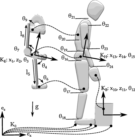
Figure 1. The human is modeled as a 10-segment 12-DoF planar mechanism, the exoskeleton is modeled as a 5-segment 9-DoF mechanism, and the box is modeled using a single 3-DoF body. Kinematic constraints between the feet and the ground, the hands and the box, the box and the ground, and the exoskeleton and the body are indicated with dashed lines. The human-only OCP uses the human and the box models, while the with-exo OCP also makes use of the exoskeleton. Note that the left and right legs have been grouped into a single leg, as have the left and right arms. The letter κ indicates a frame. The subscripts B, H, and E refer to the box, the human, and the exoskeleton models, respectively. Planar positions are indicated with x and z, angles are indicated with θ, and changes of length are indicated with an l.

The geometry of the human model is extracted from the digitization points of bony landmarks of the experimental subject. The contact points for the foot are updated such that they are slightly larger than the largest anterior and posterior center-of-pressure excursions that were recorded during the experiments. This is an important point as, in preliminary computations, we noticed that having an over-large estimation of foot size results in unrealistic movements. Mass and inertia properties were computed using Zatsiorsky’s regression equations (Zatsiorsky, 2002). Nine of the joints corresponding to the human model’s anatomical joints are actuated by torque generators. The exoskeleton is actuated by two motors that apply torques to the linkages that bridge the hip joint and the lumbar spine. These motors have upper torque bounds that correspond to one-third of the extension torque that the human subject used to lift the 15 kg box but are otherwise idealized. By using idealized motors, we compute the torque trajectories that the motors should apply to the human wearer—valuable information for the design of the exoskeleton’s actuators.

The entire exoskeleton is assumed to have a mass of 5.45 kg. The pelvis module (3.5 kg) consists of a belt (0.500 kg) upon which the three motors (1 kg each) are mounted. The next heaviest components are the torso (0.500 kg) and thigh modules (0.350 kg), which consist of a prismatic joint, a revolute joint, and a padded plate that is strapped to the body. Finally, the links that connect the pelvis module to each thigh module and the pelvis module to the torso module are assumed to be constructed out of aluminum 7178 tube (0.249 kg each) with a diameter of 1.5 cm, a wall thickness of 2 mm, and a length of 50 cm.

The differential algebraic equations (DAEs) governing this system are described as

$M(q)\stackrel{\dot{}\dot{}}{q}+c(q,\dot{q})=\tau +G{(q)}^T\mathbf{\text{λ}}$ (1)

$g(q)=0$ (2)

where q, $\dot{\mathbf{\text{q}}}$, and $\ddot{\mathbf{\text{q}}}$ are the generalized positions, velocities, and accelerations of the model, respectively; M(q) is the mass matrix, and c(q,$\dot{\mathbf{\text{q}}}$) is the vector of Coriolis and centripetal forces. The kinematic constraints between the foot and the ground, the hand and the box, and the exoskeleton and the body are in the vector g(q), while the generalized forces that these constraints apply to the system are contained in the term G(q)^T $\mathbf{\text{λ}}$ where G(q) is the Jacobian of the constraint equations g(q) with respect to q, and $\mathbf{\text{λ}}$ is a vector of Lagrange multipliers.

The vector of applied generalized forces for the human model τ_H, the exoskeleton τ_E, and the box τ_B is used to build the vector of applied generalized forces τ for the entire model. The vector of applied generalized forces for the box is empty

${\tau }_B=(0,0,0)$ (3)

since the human model grabs the box using kinematic constraints. In contrast, the vector of applied generalized forces for the human is quite full

${\tau }_H=(0,0,0,{\tau }_{16},{\tau }_{17},{\tau }_{18},{\tau }_{19},{\tau }_{20},{\tau }_{21},{\tau }_{22},{\tau }_{23},{\tau }_{24})$ (4)

where τ₁₆–τ₂₄ are the net torques generated at each joint by the flexor and extensor MTGs and the joint damping that we have added to the model. The vector of generalized forces for the exoskeleton only has two non-zero elements corresponding to the motor torques

${\tau }_E=(0,0,0,{\tau }_4,0,0,{\tau }_7,0,0).$ (5)

For the human-only OCP, only the τ_B and τ_H are used to define τ, while for the with-exo OCP, τ also contains τ_E. Note that the subscript numbering on the τ’s corresponds to the numbering used for the generalized coordinate labels in Figure 1. We use the open-source dynamics library Rigid Body Dynamics Library¹ (RBDL), an implementation of Featherstone’s order-n dynamics methods (Featherstone, 2008), developed by Felis (2017) to solve for the forward dynamics of our model.

The net torque at each of the model’s internal joints (τ₁₆…τ₂₄) is the sum of the signed flexor and extensor muscle torques acting at that joint and joint damping

${\tau }_i={\tau }_i^{\text{\hspace{0.17em}MF}}+{\tau }_i^{\text{\hspace{0.17em}ME}}-\beta {\omega }_i.$ (6)

Since each torque muscle acts in a single direction, there are two MTGs per joint, a flexor ${\tau }_i^{\text{\hspace{0.17em}MF}}$, and an extensor ${\tau }_i^{\text{\hspace{0.17em}ME}}$, for a total of 18 MTGs for the whole model.

The torque τ^M developed by a single MTG is given by

${\tau }^{\text{M}}={\tau }_{\text{o}}^{\text{\hspace{0.17em}M}}\left(u{f}^{\text{\hspace{0.17em}A}}(\theta )f^{\text{V}}(\omega )+f^{\text{PE}}(\theta )\left(1-{\beta }^{\text{PE}}\frac{\omega }{{\omega }_{\text{max}}^{\text{\hspace{0.17em}M}}}\right)\right).$ (7)

The torque developed by equation (7) is a function of the control input u from the solver (in this case mapped to the activation of the muscle), the angle θ, and angular velocity ω of the joint. The angle of the joint changes the value of f^A(θ), the active torque–angle curve, and f^PE(θ), the passive torque–angle curve. The angular velocity of the joint affects the value of f^V(ω), the torque–velocity curve, and also the damping torque of the passive element (Figure 2).

FIGURE 2

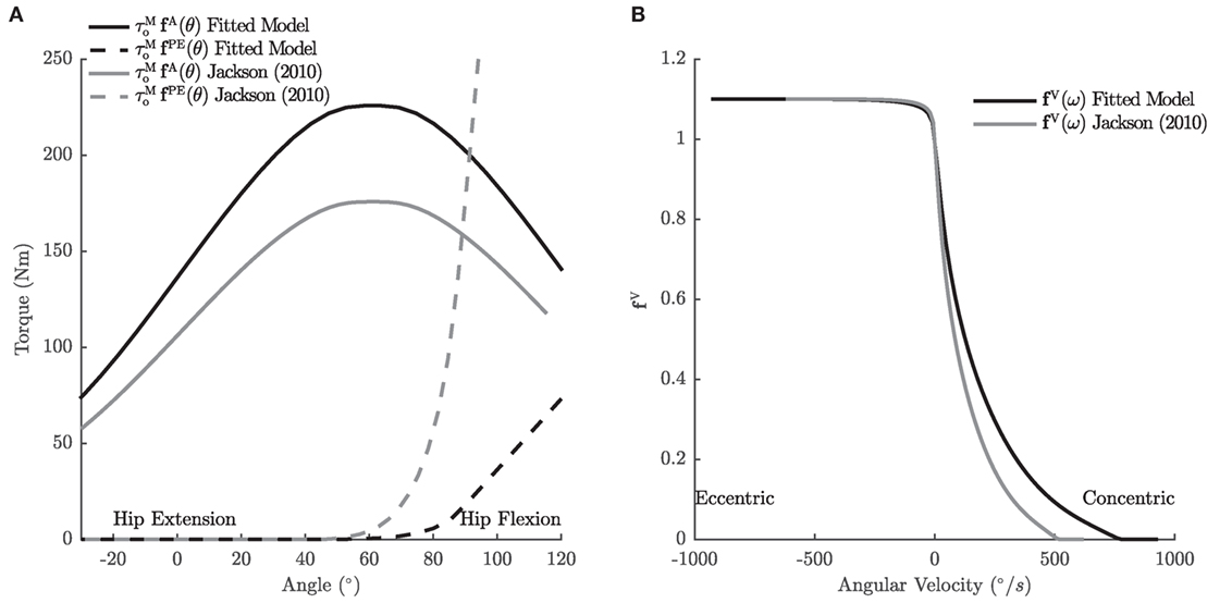
Figure 2. The torque–angle (A) and torque–velocity (B) characteristics of the hip extensors, one of the 18 MTGs used in the sagittal-plane lifting model. Jackson’s original passive torque–angle curve was applied to simulate a vault, a motion that requires far less hip flexion than a stoop. Accordingly, we shifted the passive torque–angle curve of the hip extensors to accommodate the larger hip flexion angles during the stoop motion. In addition, the strength and torque–velocity curves have been edited so that the model is strong enough to perform the lift as the experimental subject did.

A non-linear normalized damping term β^PE is added to the passive element to suppress vibration. The absence of this damping term leads to vibrations as the passive elements of the hips and back are stretched: as the stiffness of the passive element increases so too does the natural frequency of vibration of the segments to which the muscle is attached. We choose to use a non-linear damping similar to that of a Hunt and Crossley (1975) contact model because it does not noticeably increase the numerical stiffness of our dynamic equations, which is not true for a parallel damper. The value of the normalized damping coefficient β^PE is uniformly set to 0.1 for each of the muscles.

The light damping at each of the model’s joints in equation (6) is the passive damping introduced by the musculature and tissue surrounding the joint. The damping coefficient is defined as

$\beta =\eta \frac{{\tau }_{\text{o}}^{\text{\hspace{0.17em}MF}}+{\tau }_{\text{o}}^{\text{\hspace{0.17em}ME}}}{{\omega }_{\text{max}}^{\text{\hspace{0.17em}MF}}+{\omega }_{\text{max}}^{\text{\hspace{0.17em}ME}}}$ (8)

so that the amount of damping is proportional to the strength the musculature and inversely proportional to the maximum angular velocity of the musculature. The superscripts F and E designate the joint’s flexors and extensors, and η is a normalized joint damping scaling factor. Values of η of 0.2 and 0.4 effectively suppressed vibrations in the legs and arms, respectively, and result in relatively light damping coefficients ranging from β = 0.6 to 6.1 Nm s/rad.

Several literature sources are used to build the characteristic curves for the MTGs (Table 1), since there is no single source in the literature that documents all of these joints across even a single subject. The basis for the MTGs comes from Jackson (2010) who published the most complete account of the active torque–angle and torque–velocity characteristics at the hip, knee, shoulder, and wrist in an effort to simulate an elite male gymnast performing a vault. The remaining curves for ankle plantarflexion/dorsiflexion came from Anderson et al. (2007), while elbow extension/flexion, and wrist ulnar/radial deviation come from Kentel et al. (2011). Fortunately, the datasets of Anderson et al. and Kentel et al. reported curves for some of the same joints as Jackson allowing us to scale ${\tau }_{\text{o}}^{\text{\hspace{0.17em}M}}$ for the ankle, elbow, and wrist to be more consistent with the gymnast’s strength. The characteristic curves associated with the lumbar spine are derived using experimental data from Dolan et al. (1994), Raschke and Chaffin (1996), and Beimborn and Morrissey (1988).

TABLE 1

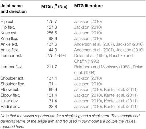
Table 1. Maximum isometric torque of the MTGs and the literature used to derive the characteristic curves for each of the MTGs.

The set of gymnast-fitted MTGs are fitted so that the model can perform the same lifting movement as the experimental subject. To fit the MTGs to the movement, we use the joint angles and velocities from an inverse kinematics analysis and the torques computed from an inverse-dynamics analysis and equation (7) to ensure that each of the muscles is flexible and strong enough to perform the same lifting motion as the experimental subject. Jackson’s hip extension passive torque–angle curve is too stiff to allow the model to perform the stoop and is accordingly scaled (Figure 2) such that the passive elasticity of the hips provides only 80% of the required extension torque that the experimental subject required to lift the box (the subject reported that his hip extensors were being strongly stretched). In addition, the force–velocity curve and maximum isometric torque of the hip extensors are adjusted such that the maximum activation of the hip extensors stayed below 75%.

In each case, fifth-order C₂ continuous (continuous to the second derivative) Bézier splines are used to approximate the active torque–angle, passive torque–angle, and torque–velocity curves provided by Jackson, Anderson et al., and Kentel et al. We approximate the curves reported in the literature because, in many cases, these curves contain C₁ discontinuities rendering them incompatible with the optimal control solution method, which requires C₂ continuity. An open-source software implementation of the MTGs is available as an add-on in RBDL.

2.2. Lifting As an Optimal Control Problem

In general, an optimal control problem is defined by the goal of identifying the vector of state x(⋅) and control functions u(⋅) that minimize the cost function

$\underset{x(\cdot ),u(\cdot ),\nu }{\text{min}}{\displaystyle \sum _{j=0}^{n_p-1}}\left({\displaystyle {\int }_{{\nu }_j}^{{\nu }_{j+1}}}{\varphi }_j(x(t),u(t),p)dt\right)$ (9)

where j iterates sequentially across the phases that begin at time ν_j and terminate at time ν_j+1. The state vector is not completely free to vary but must satisfy problem-specific constraints and the equations of motion

$\begin{array}{c}\dot{\mathbf{\text{x}}}(t)=f_j(t,\mathbf{\text{x}}(t),u(t),\mathbf{\text{p}})\text{\hspace{1em}for\hspace{1em}}t\in [{\nu }_{j-1},{\nu }_j],\\ j=1,\mathrm{\dots },n_p,{\nu }_0=0,{\nu }_{n_p}=T\end{array}$ (10)

which take the form of the DAEs in equations (1) and (2). Note that the physical quantities assigned to the state vector and the vector of control signals can vary depending on the problem formulation. Here, we use a forward-dynamics OCP, so the state vector is the positions and velocities of the multibody system, and the control vector is composed of the 18 activation signals to the MTGs. In addition, the with-exo OCP has the torque of the two motors included in its control vector.

We formulate the stooping box lift as a forward-dynamics OCP that has three separate phases (Figure 3):

• Stand to box-touch: the first phase begins with the model standing at rest and ends when the model touches the box but applies no forces to the box.

• Box-touch to box-grip: the second phase begins with the model touching the box and ends when the model is supporting the full weight of the box but otherwise applies no other forces to the box.

• Box-grip to stand: the third phase begins with the model holding the full weight of the box in the stoop position and ends when the model has lifted the box and is standing with it.

FIGURE 3

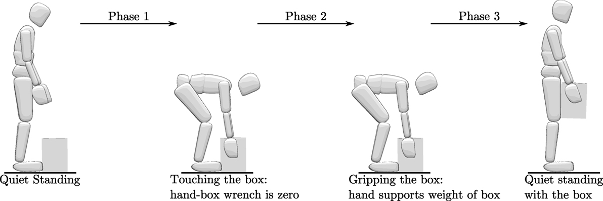
Figure 3. The stooping box lift is formulated as a three-phase OCP: stand to touching the box, touching the box to gripping the box, and finally lifting the box to a standing position.

Note that the multibody constraints between the hands and the box, and hence the underlying dynamics, between the three phases change.

We use continuous constraints

$0\le g_j(t,x(t),u(t),p)\text{\hspace{1em}for\hspace{0.17em}}t\in [{\nu }_{j-1},{\nu }_j]$ (11)

on state bounds and constraints that are specific to the movement. The limits on each state bound are chosen to be consistent with a physiological range-of-motion of each joint and more than twice as fast as joint velocities measured during the experimental recordings. The movement-specific constraints on the positions and velocities ensure that the model begins in a standing pose at rest, guides the hands to the handles of the box, and finishes the lift in a standing pose at rest. During the second-phase additional constraints are added so that the hands only apply vertical forces to the box, which begin at zero and linearly vary throughout the phase until the full weight of the box is supported by the hands. Accordingly, the box handles are placed directly above the center of mass (CoM) of the box so that it does not swing. In the third phase, additional constraints are added so that the box does not come into contact with the legs. Inequality constraints are used throughout the movement to ensure that the contact forces in the normal direction are strictly positive and that the ratio of tangential to normal forces does not exceed the coefficient of friction (we assumed a coefficient of friction of 0.8). In addition, to approximate the coordinated movement of a real lumbar spine (Wong et al., 2006), we couple the two lumbar joints so that they always have equal angular velocities. This ensures that both joints flex together and extend together. The duration of the first and final phases ν_j is free to vary and is identified during the solution process, and the duration of the second phase is fixed to match that recorded in the experiment.

To solve the optimal control problem specified in equations (9)–(11), we use a direct multiple shooting method described by Bock and Pitt (1984) and implemented in the software package MUSCOD-II developed by Leineweber et al. (2003). In this direct approach, the infinite-dimensional space of control functions u(⋅) in time is discretized using functions that provide only local support such as piecewise constant, linear, and cubic functions. State parameterization is performed by the multiple shooting technique, which transforms the OCP from an infinite-dimensional problem into a finite dimensional problem, which is then solved iteratively using a sequential quadratic programming (SQP) solver.

We solve for motions that minimize the integral of muscle activation a squared

$\underset{x(\cdot ),u(\cdot ),\nu \cdot }{\text{min}}{\displaystyle \sum _{j=0}^{n_p-1}}{\displaystyle {\int }_{{\nu }_j}^{{\nu }_{j+1}}}\left({\displaystyle \sum _{k=0}^{n_k}}{a}^T\cdot a\right)\text{\hspace{0.17em}d}t$ (12)

across all of the n_k actuated joints of the model. Objective functions consisting of activation raised to a power are commonly used in literature (Thelen et al., 2003; Damsgaard et al., 2006; Ackermann and van den Bogert, 2010) and are associated with the minimization of muscle effort (Ackermann and van den Bogert, 2010).

A naive initial solution is used to initialize the problem: positions are initialized using a linear interpolation of the experimental positions at the phase transitions, all velocities are set to zero, and all control signals are set to 0.1. The initial solution does not satisfy either the multibody constraints or the OCP constraints and is not a feasible motion. In practical terms, this is useful as it frees the developer from providing feasible initial solution for a system that may only exist as a virtual model.

Forty-two shooting and control intervals are used to discretize the lifting OCPs with 15 shooting intervals for the first and last phases and 12 shooting intervals for the middle phase. The control signal is discretized into piecewise continuous linear functions that are continuous across phases. Each shooting interval was integrated using the Runge–Kutta–Fehlberg method with an absolute and relative tolerance of 10⁻⁸. Finally, each OCP was run until the Karush–Kuhn–Tucker condition was satisfied to a tolerance of 10⁻⁵ over the course of a 3–4 h for the human-only OCP and 8–12 h for the with-exo OCP.

2.3. Experimental Measurements

The motions and ground forces of a 35-year-old male subject (mass of 81.7 kg and a height of 1.72 m) were measured as the subject stooped and picked up a 15 kg box with handles from the floor. The subject was instrumented with OptoTrack IRED marker clusters to track the three-dimensional (3D) movements of 14 body segments: head, upper torso, mid-back, pelvis, legs, shanks, feet, upper arms, and lower arms. Ground reaction forces were recorded under the subject’s feet and the box using Kistler force plates (Kistler GmbH, Germany). The recordings were conducted at Vrije Universiteit Amsterdam according to the guidelines of the Declaration of Helsinki 2013, approved by the ethics committee of Faculteit der Gedrags- en Bewegingswetenschappen (Faculty of Behavioural and Movement Sciences) and with written and informed consent from the subject.

2.4. Evaluation Procedure

We evaluate the model and the predicted results in the following ways:

1. To assess the kinematic model, we perform an inverse kinematics analysis and report the errors between the real markers on the subject and the virtual markers on the model. We report the residuals from inverse-dynamics analysis of the recorded data to assess the mass and inertia properties of the subject model. Inverse-dynamics analysis computes generalized forces that are consistent with the kinematics of the subject and the measured ground forces. Since our kinematic model has a floating pelvis frame, the inverse-dynamics results will include generalized forces between the ground frame and the pelvis frame, which should be small (as there were no external forces applied to the subject’s pelvis during the experiment). If these residual forces are small in magnitude, then we can conclude that the geometry and mass distribution of the model fits the subject well. We compare the peak lumbar-flexion angles and extension moments of our experimental subject to the data reported by Kingma et al. (2004) from 10 subjects lifting a 10.5 kg box from a height of 0.5 m using a stoop technique. All of the analysis of the subject data is performed using a human model that has two legs and arms. To assess the validity of grouping the legs and arms together (as is done for the model used in the OCPs), we report the angular difference between the hip, knee, ankle, shoulder, elbow, and wrist joints of the subject during the lift from the inverse kinematics analysis.

2. We report the joint angles and torques of the lumbar spine, hip, knee, and ankle of the human-only OCP and compare these results with the IK and ID analysis of the experimental data. Differences between the human-only OCP and analyses of the experimental data will be due to the cost function, the constraints of the OCP, and/or the MTGs.

3. We report the kinematics and kinetics of the lumbar spine, hip, knee, and ankle of the with-exo OCP and compare these results with human-only OCP to evaluate how the exoskeleton changed the motion of the model. Any differences between the human-only OCP and with-exo OCP results are entirely due to the mass of the exoskeleton and the moments that it applies to the body.

4. Finally, we report quantities useful to the design of the exoskeleton: actuator kinematics, actuator torque profiles, and human–exo interaction forces. The kinematics and torque profiles of the actuators are useful for the design of the exoskeleton’s actuators. The human–exo interaction forces are useful for the design of the linkage and the interface that transmits the support from the actuators to the wearer.

3. Results

The kinematics and dynamics of the model fit the recorded stoop motion well, with the largest kinematic errors occurring at the shoulder. The error of the inverse kinematics solution between the virtual markers on the model and measured markers is 14 ± 6.6 mm with a maximum error of 67.8 mm at the shoulders. The residual forces and moments of the inverse-dynamics analysis are 5.4 ± 3.4 N and 3.6 ± 2.5 Nm, with peaks of 19.3 N and 11.6 Nm, when the box is being picked up. The subject used in the experiments performs a stoop lift with substantially less lumbar flexion (14° vs. 39° ± 14°, Figure 4A) than was observed by Kingma et al. (2004). The net L5/S1 extension moments generated by the experimental subject are very close to those of Kingma et al.’s subjects (200 vs. 199 ± 12 Nm, Figure 4B) even though the box used in this experiment is 4.5 kg heavier. The maximum kinematic differences between the left and right legs are between 2.1° and 4.4°, while the differences between the left and right arms range between 2.8° and 15.9°.

FIGURE 4

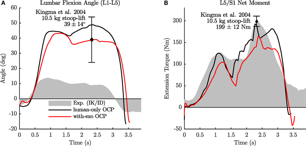
Figure 4. The lumbar-flexion angle (A) and the L5/S1 net moment (B) for the inverse-dynamics analysis of the experimental subject, the human-only OCP, and the with-exo OCP. The exoskeleton reduces the model’s lumbar-flexion angle by 6° and the peak extension moment by 28 Nm.

The human-only OCP has similar peak lumbar-flexion angles (49° vs. 39° ± 14°) and extension moments (192 vs. 199 ± 12 Nm) as the data from Kingma et al. (2004) (Figure 4). Correspondingly, the lumbar-flexion angle of the human-only OCP differs from the experimental subject (49° vs. 14°), though the angles match well at the hip. The largest differences between the human-only OCP and the experimental subject show up at the knee: the model flexes its knee more (60° vs. 49°, Figure 5B) and has different peak knee torques (55 vs. −56 Nm, Figure 5E).

FIGURE 5

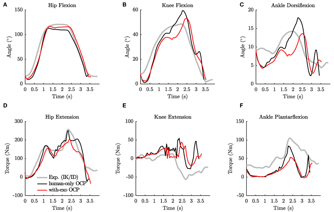
Figure 5. The joint angles of the hip (A), knee (B), and ankle (C) from the inverse-kinematics analysis of the experimental subject, the human-only OCP, and the with-exo OCP are shown in the top row. The corresponding joint torques of the hip (D), knee (E), and ankle (F) from the inverse-dynamics analysis of the experimental subject, the human-only OCP, and the with-exo OCP are shown in the bottom row.

With the ability to provide up to 67 Nm of torque (one-third of the peak lumbar extension from the ID analysis), the exoskeleton’s motors are able to reduce the lumbar flexion of the model so that the with-exo OCP solution matches the mean peak lumbar-flexion angle of Kingma et al. (2004) (43° vs. 39° ± 14°) better than the human-only OCP solution. The assistance provided by the exoskeleton reduces the peak lumbar-extension moment by 28 Nm from 192 to 164 Nm (Figure 4B). The peak flexion angles at the hip, knee, and ankle of the with-exo OCP deviate from the human-only OCP by between 4° and 7° (Figures 5A–C). The peak hip, knee, and ankle torques differ between the human-only OCP and with-exo OCP solutions by up to 47 Nm with the most pronounced differences at the hip (Figure 5D) and ankle (Figure 5F). Additional kinematic differences between the two OCP solutions and the experimental subject can be seen clearly by examining trajectories of the hands during the lift and the posture of the body when the box is picked up (Figure 6). When approaching the box (phase 1), the human-only OCP and the with-exo OCP swing the arms (slightly reducing the cost), while the experimental subject’s hands follow a more direct path. During the pickup phase (phase 3), the two OCP solutions are similar to the experimental subject.

FIGURE 6

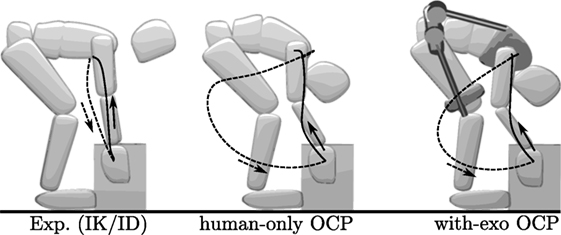
Figure 6. The experimental subject guides their hands directly to the box, while the OCP solutions swing the arms (dashed lines). During the lifting phase, experimental subject and the OCP solutions follow similar paths. The difference in the hip, knee, and lumbar-flexion angle can be seen between the experimental subject and the two OCP solutions when the box is being picked up.

The with-exo OCP solution shows that the hip actuator has to be driven with more complex signals than the lumbar actuator during the box pick up. Although both motors output the maximum torque at some point (Figure 8C), the hip motor has to undergo larger rotations (96° vs. 40°, Figure 7A) and has to sustain high velocities (145°/s, Figure 7B) for a large part of the movement. The interaction forces between the human and the exoskeleton show that the pelvis interface has to comfortably transmit large normal forces (338 N), shear forces (112 N), and torsional moments (51 Nm) to the human wearer (Figure 8A). Although the normal forces at the thigh (Figure 8B) and trunk (Figure 8C) interfaces are substantial (−184 and −216 N), the shear forces (31 and −41 N) and reaction moments (0.28 and −4.0 Nm) are small in comparison to the pelvis interface.

FIGURE 7

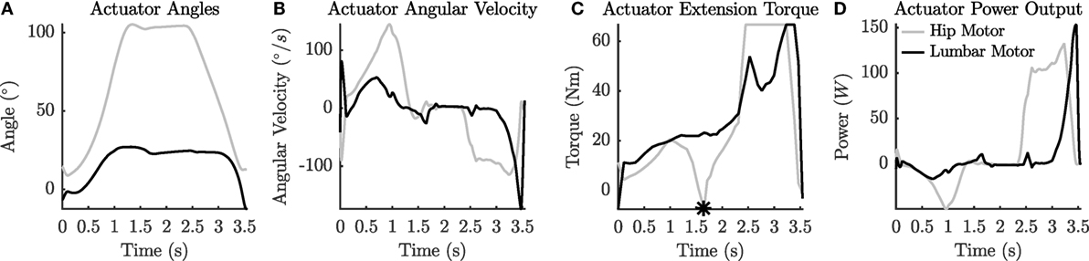
Figure 7. The motor rotor angles (A), angular velocity (B), torques (C), and power output (D), of the with-exo OCP solution.

FIGURE 8

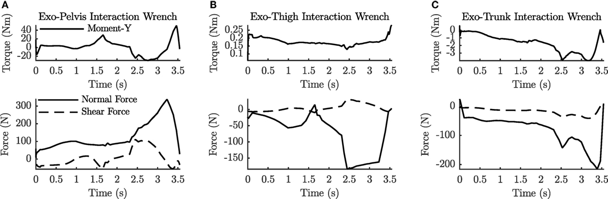
Figure 8. The net human–exo interaction forces and moments at the pelvis (A), thigh (B), and trunk (C) for the with-exo OCP.

4. Discussion

This work is motivated by the need to reduce the risk of back injury. Injury to the back is common and costly (Goetzel et al., 2003), and wearable robotic systems can decrease the risk by reducing the extension torques of the lumbar spine. The design of such systems is challenging with several aspects influencing this process: the exoskeleton can change the way the wearer moves, perhaps rendering the design ineffective; the interaction between the human and the exoskeleton may be too uncomfortable for long-term use; and/or the anticipated amount of support might differ from what the human wearer actually needs. To address some of these difficulties, the present study uses optimal control to predict the motions and forces of a dynamic model of a human lifting a 15 kg box from the floor with the aid of an exoskeleton.

We have presented an OCP of human lifting both without and with the aid of an exoskeleton. The solutions of the OCPs are physiologically realistic and dynamically consistent. The results of these simulations provide information that is useful to predict how exoskeleton might be used by the human, the requirements placed on the actuators, and finally the interaction forces between the human and the exoskeleton. The peak lumbar-flexion angles and L5/S1 extension moments predicted by the solution to the human-only OCP compare well with the 10.5 kg box stoop lift reported by Kingma et al. (2004). It is interesting to note that the L5/S1 extension moments match closely given that the box used in this work is 15 kg rather than 10.5 kg. This match likely arises because the subject used in this work is 13 cm shorter than the average subject in Kingma et al.’s study. While the predicted kinematics and loads of the lumbar spine compare favorably to the data of Kingma et al. (2004), it is clear that the cost function we have used does not do a good job of predicting the trajectory of the hands as the model moves to pick up the box (Figure 6). The solution likely converged to a motion with a large arm swing because this movement slightly reduces the muscle activity of the hip and lumbar extensors as the model approaches the box. Fortunately, the differences in arm trajectory appear to have little influence on the quantities that most affect the design of the exoskeleton: the kinematics and loads of the back and lower body.

The results indicate that indeed an exoskeleton can reduce the L5/S1 moment (Figure 4B) though this reduction might be lower than expected. Even though both the hip and lumbar motors could output a maximum torque of 67 Nm, the L5/S1 moment was only reduced by 28 Nm. Since the duration of the OCP lifts is shorter than the experimental subject, it is likely that the solver reduced the cost of the motion by lifting the box faster. Though it unclear if this will happen in real life, it is plausible: the support provided by the exoskeleton can be used to reduce the L5/S1 moment or to increase the maximum L5/S1 moment that the wearer can generate. With slight modifications to our problem formulation, we can simulate a lift in which the exoskeleton supports the wearer and also a lift in which the wearer uses exoskeleton to enhance their strength. Understanding this behavioral component in greater detail is important to the success of exoskeleton in reducing the risk of injury.

The torque waveforms computed for the hip and lumbar motors on the exoskeleton indicate that the demands on the hip and lumbar motors are quite different (Figure 7C). While the torque that the lumbar motor must provide is similar to the net torque at the L5/S1 joint of the wearer (Figure 4B), the torque that the hip motor must provide is different from the hip torque developed by the human (Figure 5D). The torque of the hip motor drops below 0 just as the box is touched because the hip MTG is deeply flexed. This deep hip flexion stretches the passive element in the MTG enough to generate the 125 Nm required to hold the position. This places an additional demand on the exoskeleton design. Not only should it be adjustable to physically fit the subject, but also it should be adjustable to fit the flexibility of the subject.

The interaction forces between the exoskeleton and the human subject indicate that extra attention must be given to the design of the interface between the exoskeleton and the pelvis. It must comfortably transmit large normal forces, shear forces, and moments to the human wearer. In our present approach, these forces are computed but do not influence the motion. For future extensions of this work, we are evaluating how the reduction of these forces could be made as a part of the OCP. As well, it would be of interest to replace our current kinematic constraints at the contact points with force-based constraints, allowing a relative movement of the exoskeleton.

We have necessarily made simplifications in modeling the human body and its interaction with the exoskeleton and the box. At the kinematic level, we have simplified the movement of the lumbar spine by approximating it as two coupled revolute joints. In addition, the shoulder joint is approximated as a revolute joint and does not include a scapulothoracic joint. Both of these approximations likely contributed to the kinematic error between the real and virtual shoulder markers. At the dynamic level, we have ignored activation dynamics of the muscles. The lack of activation dynamics has likely contributed to the relative roughness of the joint torques that appear in our results.

The solutions of the OCPs provide information that is useful during the mechanical design of the exoskeleton: the torque and power requirements of the actuators; the forces and moments that the parts of the exoskeleton must withstand; and the forces acting between the exoskeleton and the wearer. The detailed model and accurate OCP solutions that we have presented cannot be computed in real time and thus cannot be used to control the exoskeleton. However, the results of the OCPs are nonetheless useful for identifying two control strategies that the exoskeleton might employ.

One control strategy is to use the exoskeleton to compensate for the extension moment created by the weight of the upper body. To employ this strategy, the exoskeleton needs to know the mass and CoM location of the upper body and its inclination angle with respect to the vertical. The mass and CoM location of the upper body can be calculated using a few measurements of the subject’s body (Zatsiorsky, 2002) and then manually entered into the control system of the exoskeleton as part of a one-time customization of the device to the subject. The inclination angle of the wearer’s upper body with respect to the vertical can be measured using an inertial measurement unit (IMU) placed on the torso module. This strategy could reduce the L5/S1 extension moment of the subject in this study by up to 112 Nm—a 56% reduction of the L5/S1 moment required to perform the 15 kg box lift. For many applications, an exoskeleton that compensates for the weight of the torso will provide a meaningful reduction in the L5/S1 moment and thus lower the risk of low-back injury.

A second control strategy is to compensate for the weight of the upper body and the load being lifted. This strategy is more difficult to realize because the exoskeleton needs to have measurements of the kinematics of the lower body and the external forces acting on the lower body. This approach can be realized if the human subject is wearing (in addition to the exoskeleton) force-sensing insoles, goniometers at the knees, and goniometers at the ankles. Alternatively, the kinematics of the upper body could be measured along with the forces acting between the hands and the load being moved. Measuring or calculating the forces acting between the hands and the load would require the use of specialized gloves, or instrumented objects—options that are impractical for many applications. In principle, this approach could reduce the L5/S1 extension moment of the subject in this study by 199.4 Nm—100% of the L5/S1 moment required to perform the task.

While humans can adapt to working in novel environments quickly (Franklin et al., 2008), adaptation does not happen instantaneously. Thus, it is likely that an additional layer of control, beyond the two strategies discussed, will be needed so that the human has time to get used to lifting with the extra assistance. How best to adapt the online control of the exoskeleton to the human wearer remains an open area of research.

Ethics Statement

The recordings were conducted according to the guidelines of the Declaration of Helsinki 2013 and approved by the ethics committee of Faculteit der Gedrags- en Bewegingswetenschappen (Faculty of Behavioural and Movement Sciences) at Vrije Universiteit.

Author Contributions

MM undertook most of the research and the manuscript preparation. MS assisted in the research and the manuscript preparation. KM conceived of the research idea, obtained funding for the project, assisted in the work, and in the preparation of the manuscript.

Conflict of Interest Statement

The authors declare that the research was conducted in the absence of any commercial or financial relationships that could be construed as a potential conflict of interest.

Acknowledgments

We would like to thank Dr. Gert Faber and Axel Koopman at the Vrije Universiteit for their help collecting the experimental data used in this work. We also thank the Simulation and Optimization Research Group of the IWR at Heidelberg University for allowing us to work with the optimal control code MUSCOD-II. We would also like to thank the Open Access Publishing funding program from the Deutsche Forschungsgemeinschaft and Ruprecht-Karls-Universität Heidelberg for financially supporting the publication fees of this article. Finally, the financial support provided by the European Commission within the H2020 project SPEXOR (Project ID 687662) is gratefully acknowledged.

Supplementary Material

The Supplementary Material for this article can be found online at https://www.frontiersin.org/article/10.3389/frobt.2017.00041/full#supplementary-material.

Video S1. An overview of our results is presented using a side-by-side animation of the human subject, the human-only OCP, and the with-exo OCP. This animation shows that the motions between the three data sets are similar, but with a few notable differences: the OCP solutions display more rounded backs, and swing the arms through a wider path. Since the rounded backs of the OCPs compare well to the data of Kingma et al. (2004), we can conclude that the OCPs are producing movements consistent with the average subject, and that our experimental subject lifts with an usually straight back. Finally, the animation of the forces that the exoskeleton applies to the human subject shows that these forces are small until the box is lifted. During the lift, the exoskeleton applies large forces to the subject at the pelvis, the torso, and the thighs. Although these forces are mostly normal to the surfaces of the body, the shear forces at the pelvis are large enough to demand that special attention is paid to the design of the pelvis module.

Footnote

1. ^https://bitbucket.org/rbdl/rbdl.

References

Abdoli-E, M., Agnew, M. J., and Stevenson, J. M. (2006). An on-body personal lift augmentation device (PLAD) reduces EMG amplitude of erector spinae during lifting tasks. Clin. Biomech. 21, 456–465. doi: 10.1016/j.clinbiomech.2005.12.021

PubMed Abstract | CrossRef Full Text | Google Scholar

Ackermann, M., and van den Bogert, A. (2010). Optimality principles for model-based prediction of human gait. J. Biomech. 43, 1055–1060. doi:10.1016/j.jbiomech.2009.12.012

PubMed Abstract | CrossRef Full Text | Google Scholar

Anderson, D., Madigan, M., and Nussbaum, M. (2007). Maximum voluntary joint torque as a function of joint angle and angular velocity: model development and application to the lower limb. J. Biomech. 40, 3105–3113. doi:10.1016/j.jbiomech.2007.03.022

PubMed Abstract | CrossRef Full Text | Google Scholar

Anderson, F., and Pandy, M. (2001). Dynamic optimization of human walking. J. Biomech. Eng. 123, 381–390. doi:10.1115/1.1392310

PubMed Abstract | CrossRef Full Text | Google Scholar

Beimborn, D., and Morrissey, M. (1988). A review of the literature related to trunk muscle performance. Spine 13, 655–660. doi:10.1097/00007632-198813060-00010

PubMed Abstract | CrossRef Full Text | Google Scholar

Bock, H. G., and Pitt, K. J. (1984). “A multiple shooting algorithm for direct solution of optimal control problems,” in 9th IFAC World Congress (Budapest).

Google Scholar

Bosch, T., van Eck, J., Knitel, K., and de Looze, M. (2016). The effects of a passive exoskeleton on muscle activity, discomfort and endurance time in forward bending work. Appl. Ergon. 54, 212–217. doi:10.1016/j.apergo.2015.12.003

PubMed Abstract | CrossRef Full Text | Google Scholar

Coenen, P., Kingma, I., Boot, C., Twisk, J., Bongers, P., and van Dieën, J. (2013). Cumulative low back load at work as a risk factor of low back pain: a prospective cohort study. J. Occup. Rehabil. 23, 11–18. doi:10.1007/s10926-012-9375-z

PubMed Abstract | CrossRef Full Text | Google Scholar

Damsgaard, M., Rasmussen, J., Christensen, S., Surma, E., and de Zee, M. (2006). Analysis of musculoskeletal systems in the AnyBody modeling system. Simul. Model. Pract. Theory 14, 1100–1111. doi:10.1016/j.simpat.2006.09.001

CrossRef Full Text | Google Scholar

Dolan, P., Mannion, A., and Adams, M. (1994). Passive tissues help the back muscles to generate extensor moments during lifting. J. Biomech. 27, 1077–1085. doi:10.1016/0021-9290(94)90224-0

PubMed Abstract | CrossRef Full Text | Google Scholar

Dorn, T., Wang, J., Hicks, J., and Delp, S. (2015). Predictive simulation generates human adaptations during loaded and inclined walking. PLoS ONE 10:e0121407. doi:10.1371/journal.pone.0121407

PubMed Abstract | CrossRef Full Text | Google Scholar

Featherstone, R. (1983). The calculation of robot dynamics using articulated-body inertias. Int. J. Robot. Res. 2, 13–30. doi:10.1177/027836498300200102

CrossRef Full Text | Google Scholar

Featherstone, R. (2008). Rigid Body Dynamics Algorithms. New York: Springer.

Google Scholar

Felis, M. L. (2017). RBDL: an efficient rigid-body dynamics library using recursive algorithms. Auton. Robots 41, 495–511. doi:10.1007/s10514-016-9574-0

CrossRef Full Text | Google Scholar

Franklin, D. W., Burdet, E., Tee, K. P., Osu, R., Chew, C., Milner, T. E., et al. (2008). CNS learns stable, accurate, and efficient movements using a simple algorithm. J. Neurosci. 28, 11165–11173. doi:10.1523/JNEUROSCI.3099-08.2008

PubMed Abstract | CrossRef Full Text | Google Scholar

Goetzel, R. Z., Hawkins, K., Ozminkowski, R. J., and Wang, S. (2003). The health and productivity cost burden of the “top 10” physical and mental health conditions affecting six large U.S. employers in 1999. J. Occup. Environ. Med. 45, 5–14. doi:10.1097/00043764-200301000-00007

CrossRef Full Text | Google Scholar

Hiley, M., Jackson, M., and Yeadon, M. (2015). Optimal technique for maximal forward rotating vaults in men’s gymnastics. Hum. Mov. Sci. 42, 117–131. doi:10.1016/j.humov.2015.05.006

CrossRef Full Text | Google Scholar

Hunt, K., and Crossley, F. (1975). Coefficient of restitution interpreted as damping in vibroimpact. Trans. ASME J. Appl. Mech. 42, 440–445. doi:10.1115/1.3423596

CrossRef Full Text | Google Scholar

Jackson, M. (2010). The Mechanics of the Table Contact Phase of Gymnastics Vaulting. Ph.D. thesis, Loughborough University, Loughborough, UK.

Google Scholar

Jain, A. (1991). Unified formulation of dynamics for serial rigid multibody systems. J. Guid. Control Dyn. 14, 531–542. doi:10.2514/3.20672

CrossRef Full Text | Google Scholar

Kentel, B., King, M., and Mitchell, S. (2011). Evaluation of a subject-specific, torque-driven computer simulation model of one-handed tennis backhand ground strokes. J. Appl. Biomech. 27, 345–354. doi:10.1123/jab.27.4.345

PubMed Abstract | CrossRef Full Text | Google Scholar

Kingma, I., Bosch, T., Bruins, L., and Van Dieën, J. (2004). Foot positioning instruction, initial vertical load position and lifting technique: effects on low back loading. Ergonomics 47, 1365–1385. doi:10.1080/00140130410001714742

PubMed Abstract | CrossRef Full Text | Google Scholar

Koch, H., and Mombaur, K. (2015). “ExoOpt a framework for patient cetered design optimization of lower limb exoskeletons,” in IEEE International Conference on Rehabilitation Robotics (Singapore: IEEE).

Google Scholar

Koschorreck, J., and Mombaur, K. (2011). Modeling and optimal control of human platform diving with somersaults and twists. Optim. Eng. 13, 29–56. doi:10.1007/s11081-011-9169-8

CrossRef Full Text | Google Scholar

Leineweber, D., Schäfer, A., Bock, H., and Schlöder, J. (2003). An efficient multiple shooting based reduced SQP strategy for large-scale dynamic process optimization: part II: software aspects and applications. Comput. Chem. Eng. 27, 167–174. doi:10.1016/S0098-1354(02)00158-8

CrossRef Full Text | Google Scholar

Luo, Z., and Yu, Y. (2013). “Wearable stooping-assist device in reducing risk of low back disorders during stooped work,” in 2013 IEEE International Conference on Mechatronics and Automation (Takamatsu, Japan: IEEE), 230–236.

Google Scholar

Manns, P., Sreenivasa, M., Millard, M., and Mombaur, K. (2017). Motion optimization and parameter identification for a human and lower-back exoskeleton model. IEEE Robot. Autom. Lett. 2, 1564–1570. doi:10.1109/LRA.2017.2676355

CrossRef Full Text | Google Scholar

McGill, S. M. (1997). The biomechanics of low back injury: implications on current practice in industry and the clinic. J. Biomech. 30, 465–475. doi:10.1016/S0021-9290(96)00172-8

PubMed Abstract | CrossRef Full Text | Google Scholar

Naruse, K., Kawai, S., and Kukichi, T. (2005). “Three-dimensional lifting-up motion analysis for wearable power assist device of lower back support,” in 2005 IEEE/RSJ International Conference on Intelligent Robots and Systems (Edmonton, Canada: IEEE), 2959–2964.

Google Scholar

Raschke, U., and Chaffin, D. (1996). Support for a linear length-tension relation of the torso extensor muscles: an investigation of the length and velocity EMG-force relationships. J. Biomech. 29, 1597–1604. doi:10.1016/S0021-9290(96)80011-X

PubMed Abstract | CrossRef Full Text | Google Scholar

Schemschat, R., Clever, D., Felis, M., Chiovetto, E., Giese, M., and Mombaur, K. (2016). “Joint torque analysis of push recovery motions during human walking,” in 2016 6th IEEE International Conference on Biomedical Robotics and Biomechatronics (BioRob) (Singapore, Singapore: IEEE), 133–139.

Google Scholar

Schultz, G., and Mombaur, K. (2010). Modeling and optimal control of human-like running. IEEE/ASME Trans. Mechatron. 15, 783–792. doi:10.1109/TMECH.2009.2035112

CrossRef Full Text | Google Scholar

Thelen, D., Anderson, F., and Delp, S. (2003). Generating dynamic simulations of movement using computed muscle control. J. Biomech. 36, 321–328. doi:10.1016/S0021-9290(02)00432-3

PubMed Abstract | CrossRef Full Text | Google Scholar

Ulrey, B., and Fathallah, F. (2013). Effect of a personal weight transfer device on muscle activities and joint flexions in the stooped posture. J. Electromyogr. Kinesiol. 23, 195–205. doi:10.1016/j.jelekin.2012.08.014

CrossRef Full Text | Google Scholar

van Dieën, J., and Kingma, I. (2005). Effects of antagonistic co-contraction on differences between electromyography based and optimization based estimates of spinal forces. Ergonomics 48, 411–426. doi:10.1080/00140130512331332918

PubMed Abstract | CrossRef Full Text | Google Scholar

van Dieën, J. H., Hoozemans, M. J., and Toussaint, H. M. (1999). Stoop or squat: a review of biomechanical studies on lifting technique. Clin. Biomech. 14, 685–696. doi:10.1016/S0268-0033(99)00031-5

PubMed Abstract | CrossRef Full Text | Google Scholar

von Stryk, O. (1993). Numerical solution of optimal control problems by direct collocation in Optimal Control. ISNM International Series of Numerical Mathematics, Vol. 111. eds. R. Bulirsch, A. Miele, J. Stoer, and K. Well (Basel: Birkhäuser), 129–143.

Google Scholar

Wong, K. W., Luk, K. D., Leong, J. C., Wong, S. F., and Wong, K. K. (2006). Continuous dynamic spinal motion analysis. Spine 31, 414–419. doi:10.1097/01.brs.0000199955.87517.82

PubMed Abstract | CrossRef Full Text | Google Scholar

Zatsiorsky, V. (2002). Kinetics of Human Motion. Champaign, USA: Human Kinetics.

Google Scholar