 Nitin Sharma
 Nicholas Andrew Kirsch
 Naji A. Alibeji
 Warren E. Dixon
- 1Department of Mechanical Engineering and Materials Science, University of Pittsburgh, Pittsburgh, PA, United States
- 2IAM Robotics, Pittsburgh, PA, United States
- 3Department of Biomedical Engineering, Case Western Reserve University, Cleveland, OH, United States
- 4Department of Mechanical and Aerospace Engineering, University of Florida, Gainesville, FL, United States
Neuromuscular electrical stimulation (NMES) is a promising technique to artificially activate muscles as a means to potentially restore the capability to perform functional tasks in persons with neurological disorders. A pervasive problem with NMES is that overstimulation of the muscle (among other factors) leads to rapid muscle fatigue, which limits the use of clinical and commercial NMES systems. The objective of this article is to develop an NMES controller that incorporates the effects of muscle fatigue during NMES-induced non-isometric contraction of the human quadriceps femoris muscle. Our previous work that used the RISE class of non-linear controllers cannot accommodate fatigue and muscle activation dynamics. A totally new control design approach and associated stability proof is required to derive a new class of NMES control design that accounts for muscle fatigue dynamics and a first-order activation dynamics, in addition to the second-order musculoskeletal dynamics. Motivated from a control method for robotic systems in a strict-feedback form, a backstepping based-non-linear NMES controller was designed to accommodate for the additional muscle activation dynamics. Further, experimentally identified estimates of the fatigue and activation dynamics were incorporated in the control design. The developed controller uses a neural network-based estimate of the musculoskeletal dynamics and error due to fatigue estimation. A globally uniformly ultimately bounded stability is proven the new controller that accounts for an uncertain non-linear muscle model and bounded non-linear disturbances (e.g., spasticity and changing load dynamics). The developed controller was validated through experiments on the left and right legs of 3 able-bodied subjects and was compared with a proportional-derivative (PD) controller and a PD augmented with a neural network. The statistical analysis showed improved control performance compared with the PD controller.
1. Introduction
Neuromuscular electrical stimulation (NMES) is a promising technique that produces a muscle contraction through the application of an external electrical current. It has the potential to restore functional tasks in persons with upper motor neuron lesions. Numerous technical challenges such as non-linearity associated with muscle force generation, uncertainties in muscle physiology (e.g., calcium dynamics, pH, and muscle architecture), muscle fatigue, and time delays hinder an effective application of NMES to produce a desired muscle contraction.
In light of these challenges, researchers have explored several control strategies to develop effective NMES controllers; e.g., linear PID-based pure feedback methods (cf., Abbas and Chizeck, 1991; Lan et al., 1991a,b; Lynch and Popovic, 2012; Klauer et al., 2014; and the references therein), neural network (NN) based controllers (cf., Tong and Granat, 1999; Kordylewski and Graupe, 2001; Sepulveda, 2003; Zhang and Zhu, 2004; Giuffrida and Crago, 2005; Wang et al., 2013; and the references therein), and combined feedback and feedforward methods (Chang et al., 1997; Ferrarin et al., 2001; Chen et al., 2005; Ajoudani and Erfanian, 2009; Freeman et al., 2009; Freeman, 2014). Recently, Lyapunov-based techniques were utilized in Schauer et al. (2005), Sharma et al. (2009b, 2011, 2012), and Downey et al. (2015) to design NMES controllers and prove asymptotic stability for an uncertain non-linear muscle model. While efforts, such as Sharma et al. (2009b, 2011, 2012), Wang et al. (2013), and Cheng et al. (2016), provide an inroad to the development of analytical NMES controllers for the non-linear muscle, these results do not account for muscle fatigue, which is a primary factor to consider to yield some functional results in many rehabilitation applications.
Heuristically, muscle fatigue is a decrease in the muscle force output for a given input and is a complex, multifactorial phenomenon (Levy et al., 1990; Russ et al., 2002). Some of the factors associated with the onset of fatigue are failure of excitation of motor neurons, impairment of action potential propagation in the muscle membrane and conductivity of sarcoplasmic reticulum due to Ca2+ ion concentration, and the change in concentration of catabolites and metabolites (Asmussen, 1979). Factors such as the stimulation method, muscle fiber composition, state of training of the muscle, and the duration and task to be performed have been noticed to affect fatigue during NMES. Given the impact of fatigue during NMES, researchers have proposed different stimulation strategies (Binder-Macleod et al., 2002; Maladen et al., 2007; Downey et al., 2011, 2015) to delay the onset of fatigue such as choosing different stimulation patterns and parameters, improving fatigue resistance through muscle retraining, sequential stimulation, and size order recruitment.
Controllers can be designed with some feedforward knowledge to approximate the fatigue onset or employ some assumed mathematical model of the fatigue in the control design. Researchers in Giat et al. (1993), Riener et al. (1996), Riener and Fuhr (1998), and Ding et al. (2002a,b) developed various mathematical models for fatigue. In Giat et al. (1993), a musculotendon model for a quadriceps muscle undergoing isometric contractions during NMES was proposed. The model incorporated fatigue based on the intracellular pH level where fatigue parameters for a typical subject were found through metabolic information, experimentation, and curve fitting. A more general mathematical model for dynamic fatigue defined as a function of the Ca2+ dynamics was proposed in Riener et al. (1996) and Riener and Fuhr (1998). Fatigue was introduced in the musculoskeletal dynamics as a fitness variable that varies as electrically stimulated muscles fatigue or recover. The fatigue time parameters were estimated from stimulation experiments. Models in Ding et al. (2002a,b) predict force due to the effect of stimulation patterns and resting times with changing physiological conditions, where model parameterization required investigating experimental forces generated from a standardized stimulation protocol.
Although the aforementioned mathematical models for fatigue prediction are available, few researchers have utilized such models for closed-loop NMES control. Results in Riener and Fuhr (1998) and Jezernik et al. (2004) use the fatigue model proposed in Riener et al. (1996) and Riener and Fuhr (1998) for NMES controllers, where patient specific parameters (e.g., fatigue time constants) are assumed to be known, along with exact model knowledge of the calcium dynamics. The difficulty involved in the control design using calcium dynamics, or intracellular pH level, is that these states cannot be measured for real-time control. An ad hoc method to obtain states such as the calcium dynamics or pH level for real-time would be to estimate states from a first or second-order differential equation that acts as a phenomenological fatigue model (cf., Giat et al., 1993; Riener and Fuhr, 1998; Jezernik et al., 2004), where the parameters in the equations are estimated from experimentation or are based on data from past studies.
The focus of this article is to address muscle fatigue by incorporating an uncertain fatigue model (i.e., the model developed in Riener et al. (1996)) in the NMES controller. Unlike our previous NMES controllers (Sharma et al., 2009b, 2011, 2012; Wang et al., 2013; Downey et al., 2015), the controller presented here models the presence of muscle fatigue and compensates for the diminishing control effectiveness caused by NMES-induced muscle fatigue. Our previous work used the RISE-type controllers. The stability and control design approach used for these type of controllers are incompatible when fatigue and muscle activation dynamics are incorporated. The continuous NN-based controller is proven (through a Lyapunov-based stability analysis) to yield a globally uniformly ultimately bounded stability result despite the uncertain non-linear muscle model and the presence of additive bounded disturbances (e.g., muscle spasticity, changing loads in functional tasks, and delays). This article extends the preliminary results presented in Sharma et al. (2009a), Sharma (2010), and Kirsch (2016) through experimental validation of the new controller. In Sharma et al. (2009a) and Sharma (2010), how this controller might be implemented was left unclear because the developed controller requires muscle activation variable that cannot be directly measured. In this article, a procedure for determining the parameters of muscle activation and fatigue dynamics are presented accompanied with the experimental validation of the developed controller.
2. Muscle Activation and Limb Model
The following model development represents the musculoskeletal dynamics during NMES applied to a person’s quadriceps muscle. The total musculoskeletal knee-joint model can be categorized into body segmental dynamics and muscle activation and contraction dynamics. The muscle activation and contraction dynamics model the force generation in the muscle, while the body segmental dynamics considers the active moment and passive joint moments acting on the knee. This is illustrated in Figure 1.
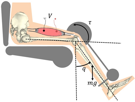
Figure 1. Electrical stimulation of the quadriceps causes the muscle to contract and shorten. This creates a torque at the knee joint, causing a knee extension motion.
2.1. Contraction and Activation Dynamics
The torque produced about the knee is generated through muscle forces that are elicited by NMES. The active moment generating force at the knee joint is the is related to the muscle force as
where ς ∈ ℝ denotes a positive moment arm that changes with the extension and flexion of the leg and a(q(t)) ∈ ℝ is defined as the pennation angle between the tendon and the direction of the muscle fibers. The pennation angle increases as the muscle shortens and varies between the different muscle types, but ranges from approximately 0–30°(Winter, 2009). As given in Riener and Fuhr (1998), the moment arm can be defined as
where c1, c2 ∈ ℝ+ are positive constants. The moment arm is considered as a continuously differentiable, positive, and bounded function with a bounded first time derivative. The muscle force F ∈ ℝ in equation (1) is defined as (Riener and Fuhr, 1998)
where Fm ∈ ℝ is the constant maximum isometric force generated by the muscle. The uncertain non-linear functions η1: ℝ → ℝ in equation (2) is the force–length relationship, defined as (Hatze, 1977)
where b ∈ ℝ is a constant that denotes the unknown shape factor, l ∈ ℝ denotes the length of the muscle, denotes the optimal muscle length (i.e., η1 is greatest for ). In equation (2), η2: ℝ → ℝ is the force–velocity relationship, defined as (Happee, 1994)
where is an unknown non-negative normalized velocity with respect to the maximal contraction velocity of the muscle, and d1, d2, d3, d4 ∈ ℝ+ are unknown, positive constants.
The force–length function, η1 in equation (3), is a Gaussian function. Therefore, for all real values of l the force–length function can be bounded by a constant, which we will define to be εη1 . This lower bound is practical in the sense that muscles are capable of generating a contractile force for any real muscle length. Similarly, the force–velocity function η2 in equation (4) is lower bounded by a constant εη2 . The lower bound on the force–velocity relationship is practical in the sense that η → 0 as the muscle shortening velocity (a concentric contraction) nears infinity.
The definitions in equation (3) are not directly used in the control development. Instead, the structure of the relationships in equation (3) is used to conclude that η1 and η2 are continuously differentiable, non-zero, positive, and bounded functions.
The muscle force in equation (2) is coupled to the stimulation control input v ∈ ℝ through an intermediate normalized muscle activation variable x ∈ ℝ. The muscle activation variable is governed by the following differential equation (Zajac, 1989)
where w ∈ ℝ is the constant, unknown natural frequency of the calcium dynamics. The function sat[v] ∈ ℝ (i.e., recruitment curve) is denoted by a piecewise linear function as (Schauer et al., 2005)
where vmin ∈ ℝ is the minimum stimulation required to generate noticeable movement or force production in a muscle and vmax ∈ ℝ is the stimulation input to the muscle at which no considerable increase in force or movement is observed. Based on equations (5) and (6), a linear differential inequality can be developed to show that x ∈ [0, 1]. Muscle fatigue is included in equation (2) through the invertible, positive, bounded fatigue term φ ∈ ℝ that is generated from the first-order differential equation as (Riener et al., 1996)
where φmin ∈ [0, 1] is the unknown minimum fatigue constant of the muscle and Tf, Tr ∈ ℝ+ are unknown time constants for fatigue and recovery in the muscle, respectively. Because x ∈ [0, 1] it can be shown that φ ∈ [φmin, 1], where φ = 1 when the muscle is fully rested, and φ = φmin when the muscle is fully fatigued. For x = 0, equation (7) can be reduced to , which has the solution φ(t) = 1 + (φr0 − 1)e−t∕Tr that converges to 1 as t → ∞. For x = 1, equation (7) can be reduced to , which has the solution that converges to φmin as t → ∞. Since x ∈ [0, 1] and because equation (7) is a first-order differential equation, the solutions of φ at the bounds of x results in φ being bounded as φ ∈ [φmin, 1].
2.2. Body Segmental Dynamics (Knee Dynamics)
The total knee-joint dynamics in the sagittal plane can be modeled as (Schauer et al., 2005)
In equation (8), J ∈ ℝ+ denotes the inertia of the combined shank and foot, Me ∈ ℝ denotes the elastic effects due to joint stiffness, Mg ∈ ℝ denotes the gravitational component, Mv ∈ ℝ denotes the viscous effects due to damping in the musculotendon complex (Ferrarin and Pedotti, 2000), τd ∈ ℝ is an unknown bounded exogenous disturbance that represents an unmodeled reflex activation of the muscle (e.g., muscle spasticity) and other unknown unmodeled phenomena (e.g., changing loads), and τ ∈ ℝ denotes the torque produced at the knee joint due to NMES. In the subsequent development, the unknown disturbance τd is assumed to be bounded, which is reasonable for typical disturbances such as muscle spasticity and load changes during functional tasks. The definitions of Me, Mg, and Mv are given in our previous work (Sharma et al., 2009a,b, 2011, 2012).
3. Control Development
The objective is to develop an NMES controller to produce a knee torque trajectory that will enable a person’s shank to track a desired trajectory, denoted by qd ∈ ℝ, despite uncertain fatigue effects and coupled muscle force and calcium dynamics. A Lyapunov redesign approach is used, where the control development and stability analysis are performed at the same time, to design control and update laws. Without loss of generality, the developed controller is applicable to different stimulation protocols (i.e., voltage, frequency, or pulse width modulation). To quantify the objective, a position tracking error, denoted by e ∈ ℝ, is defined as
where qd is designed such that , where denotes the ith derivative for i = 0, 1, 2, 3, 4. To facilitate the subsequent analysis, a filtered tracking error, denoted by r ∈ ℝ, is defined as
where α ∈ ℝ denotes a positive constant.
3.1. Open-Loop Error System
The open-loop tracking error system is developed by taking the time derivative of equation (10), multiplying the resulting expression by J, and then utilizing the expressions in equations (1), (2), (8), and (9) to yield
where the auxiliary term ρ ∈ ℝ is defined as
After multiplying equation (11) by ρ−1, the following expression is obtained:
where Jp, τdp, Lρ ∈ ℝ are defined as
Property 1: Based on the assumptions and properties in Section 2, ρ is continuously differentiable, positive, and bounded. The first time derivatives of ρ and exist and are bounded. The inertia function Jp is positive definite and can be upper and lower bounded as
where a1, a2 ∈ ℝ+ are some known positive constants. Based on the boundedness of ρ, , and
where ξj, ξτ ∈ ℝ+ are some known positive constants.
Based on equation (7) a positive estimate is generated as
where denote constant, estimates of the time constants Tf and Tr, respectively. is a non-zero known positive constant that is an estimate of φmin, and is the estimated normalized muscle activation variable which is generated based on equation (5) as
where denotes the constant best-guess estimate of w, the unknown natural frequency of the calcium dynamics. The estimated function is upper bounded by a positive constant . Specifically, can be determined as
The differential equation (15) ensures that remains strictly positive. Based on equations (6) and (16), a linear differential inequality can be developed to show that .
In the next step, the open-loop error dynamics in equation (12) is algebraically manipulated to separate a term that will be estimated by the NN, and also to obtain functions that represent errors due to estimated fatigue and muscle activation variables. Thus, the open-loop error dynamics can be expressed as
where the auxiliary function S ∈ ℝ that will be estimated by the NN is defined as
and the error functions φe, , are defined as
Since φ is a bounded function, the error function φe can be upper bounded as
where ξφ ∈ ℝ is some known positive constant. The auxiliary function S can be represented by a three-layer NN as
where y ∈ ℝ7 is defined as
and are bounded constant ideal weight matrices for the first-to-second and second-to-third layers, respectively, where N1 is the number of neurons in the input layer, N2 is the number of neurons in the hidden layer, and n is the number of neurons in the output layer. The sigmoid activation function in equation (21) is denoted by , and ϵ ∈ ℝn is the functional reconstruction error, which can be upper bounded by a constant as
The additional term “1” in the input vector y and activation term σ enables the activation function thresholds to be included as the first columns of the weight matrices (Lewis et al., 2002). Thus, any tuning of W and U also includes tuning the thresholds.
3.2. Closed-Loop Error System
Since a direct control input does not appear in the open-loop system in equation (17), a backstepping-based approach is used to inject a virtual control input xd ∈ ℝ (i.e., desired muscle activation) as
Based on equation (24), the virtual control input is designed as a three-layer NN feedforward term plus a feedback term as
where and are positive constant gains. The feedforward NN component in equation (25), denoted by is generated as
where and are estimates of the ideal weight matrices. Estimates for the NN weights in equation (26) are generated online using a projection algorithm (Krstic et al., 1995) as
where and are constant, positive definite, symmetric gain matrices. The closed-loop tracking error system can be developed by substituting equation (25) into equation (24) as
where is defined as
and ex ∈ ℝ is the backstepping error defined as
After writing the definitions of S and in terms of ideal and estimated NN weights, the closed-loop system can be expressed as
where is defined as , the notations and , , for a given y is defined as . The Taylor series expansion for σ(UTy), (Lewis et al., 2002) for a given y, is , where and can be used to write as , where . Using this expression, equation (30) can be rewritten as
where the unmeasurable auxiliary term N ∈ ℝ is introduced to facilitate subsequent stability analysis and is defined as
where is defined as . Based on equations (14), (20), (23), and (27), the fact that x, , and the assumption that desired trajectories are bounded, the following inequality can be developed (Lewis, 1996):
where ζi ∈ ℝ+ for (i = 1,2) are known positive constants, and z ∈ ℝ2 is defined as
3.3. Backstepping Error System
To facilitate the subsequent stability analysis, the time derivative of the backstepping error (equation (29)) can be determined by using equation (16) as
Due to the input saturation function in this system, which is expressed in equation (6), we want v ∈ [vmin, vmax]. Based on equations (6) and (33), the stimulation control input is designed as
where Δv = vmax − vmin and 1; k ∈ ℝ+ denotes a positive constant adjustable control gain. For , (i.e., when ), equation (33) becomes
Note that equation (35) is valid only for the case where the control signal in equation (34) is not saturated (i.e., ). In other words, equation (35) is valid for
The controller given in equation (34) is the actual stimulation input to the muscle. The variables vmax and vmin are saturation and threshold stimulation inputs, respectively and can be selected appropriately, depending on the type of modulation employed. For example, the controller can be implemented as a voltage modulation or current modulation or pulsewidth modulation controller. Mainly a PD + NN signal (with fatigue compensation) is used as a virtual control input and due to the use of backstepping approach, the actual controller uses the time derivative of the virtual control input, in addition to other signals such as , , r, and ex. A block diagram describing the controller is shown in Figure 2.
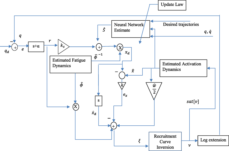
Figure 2. A block diagram describing the control implementation.
4. Stability Analysis
Theorem 1. The controller given in equations (25) and (34) ensures that all system signals are bounded under closed-loop operation and that the position tracking error is uniformly ultimately bounded in the sense that
provided that the bound in equation (36) is satisfied (i.e., the input is not saturated), and the control gains α (introduced in equation (10)) and (subsequently introduced) are selected according to the following sufficient condition:
where ϵ0, ϵ1, ϵ2 ∈ ℝ+ denote positive constants, and ζ2 is a known positive constant introduced in equation (32). Proof : See Appendix.
5. Parameter Estimation
The controller given in equation (34) is a robust and adaptive controller; i.e., many of the aforementioned model parameters in Section 2 are not required to be known for the control implementation. The controller, however, uses estimates of the muscle activation dynamics in equation (5), the muscle recruitment threshold and saturation in equation (6), and the fatigue variable in equation (7). These are estimates of the following parameters: threshold (vmin), saturation (vmax), natural frequency of the calcium dynamics (w), muscle fatigue state (φ), and the muscle activation (x). This section describes the procedures that were used to estimate these parameters. The parameter estimation was performed on the right and left legs of three able-bodied subjects.2 The results of the parameter estimation for Subject 1 are presented in this section to demonstrate the procedure and accuracy of the parameter estimation. The parameters estimated for all participants can be found in the following section. During the parameter estimation procedures the participants were asked to relax and avoid any voluntary contractions that might influence the results during electrical stimulation.
All of the procedures discussed in this section were performed in a leg extension machine fitted with a load cell that held the leg in an isometric configuration at approximately 90° of knee flexion, as shown in Figure 3. The isometric joint torque was computed from the force measured by the load cell (Omega Engineering Inc., USA) and the moment arm of the leg extension machine. Isometric tests were used because it can be shown that in an isometric contraction the joint torque normalized by the maximum torque that can be produced at that joint angle is equal to the product of the muscle activation and the fatigue state (i.e., for isometric contraction η2 = 1 and from equation (2)). The quadriceps muscles were stimulated using an FNS-16 Multi-Channel Stimulator (CWE Inc., USA), which is current amplitude controlled with a resolution of 0.1 mA and maximum current amplitude of 100 mA. The FNS-16 was modified from the standard model to increase the amplitude range from 20 to 100 mA, as NMES of human quadriceps muscles typically require current amplitudes in the range of 20–100 mA to achieve a significant muscle contraction. A current amplitude controlled 35 Hz pulse train with a pulse width of 400 μs was used. The stimulation train was delivered to the quadriceps muscles through 2.75" × 5" self-adhesive NMES stimulating electrodes (Dura-Stick plus). The muscle activation and fatigue parameters estimated in this section are dependent on the stimulation parameters used during identification. Therefore, it is important to note that the stimulation parameters (frequency and pulse width) used during the parameter estimation procedures are same as the stimulation parameters during the controller validation experiments. It is also important to note that the parameters can change with placement of the electrodes. To address this issue the electrode placement procedures in (https://www.axelgaard.com/Education) were used, and the electrode placements were noted for each subject to facilitate consistency between all procedures.
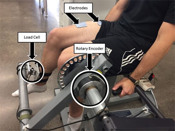
Figure 3. Test setup for estimating fatigue and activation dynamics. The isometric joint torque, produced by stimulation of the quadriceps muscles, was measured by keeping the arm of the leg extension machine fixed and holding the subject’s leg in place with a load cell. The test setup was also used to validate the developed controller for NMES knee extension tracking experiments. A rotary encoder was used to measure the knee-joint angle. The depicted individual provided written and informed consent for the publication of this image.
Pulse trains of increasing current amplitude were used to determine the saturation and threshold current amplitudes. The threshold current amplitude is the amplitude that produces the first noticeable isometric joint torque, and the saturation current amplitude is the minimum amplitude that produces no further significant increase in joint torque. One-second long stimulation pulse trains were used to minimize muscle fatigue that may occur during the procedure. From the results shown in Figure 4A, the threshold amplitude was determined to be 33 mA. The increase in the isometric torque was found to be an insignificant (much less than 1 Nm) at stimulation amplitudes beyond 77 mA. Therefore, the saturation current amplitude was chosen as 77 mA.
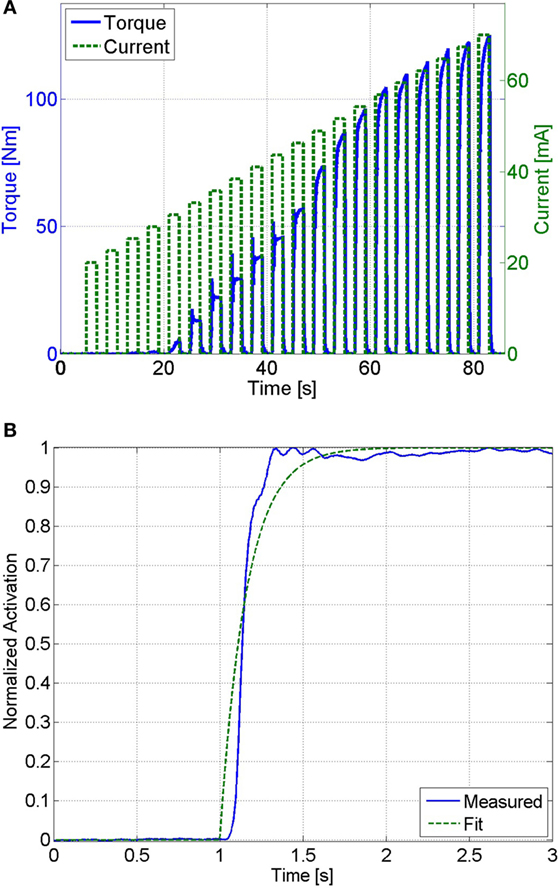
Figure 4. (A) The threshold and saturation current amplitudes were determined from this plot. The threshold amplitude was determined to be 33 mA, and the saturation amplitude was determined to be 77 mA. (B) This plot shows the measured muscle activation and the best fit first-order response for a unit step input, which has an RMS error of 0.045. The first-order response has a time constant of 0.16 s, which corresponds to a calcium dynamics natural frequency of 12.5 HZ.
To generate an estimate of the muscle activation (Ca2+) dynamics in equation (16), its natural frequency was estimated. The muscle activation dynamics were modeled as a first-order system with sat[v] as the input and 2/w as the time constant (see equation (16)). Therefore, the estimated natural frequency, , can be determined by solving for the time constant of a first-order system that best matched the response of the muscle activation. Assuming that muscle fatigue does not occur (φ = 1) the normalized load cell data can be used as a measurement of muscle activation (i.e., ). The unit step response of muscle activation dynamics were tested by stimulating the subject at the saturation level (sat[v] = 1) and using the load cell data, normalized by the maximum isometric force measured at that position (Fmη1), as a measurement of muscle activation. This procedure was conducted 3 min after the previous procedure to ensure that the subject was not fatigued. This procedure was only conducted once, since further trials would induce fatigue. Any induced muscle fatigue would cause the isometric contraction to not reach a normalized activation of one, which would affect the parameter estimation. An optimization method was then used to solve for the first-order system with a time constant that best matches the response measured by the load cell. MATLAB’s fmincon function (MathWorks, Boston, MA, USA), using an interior-point algorithm, was used to perform the optimizations to estimate the muscle activation time constant for each of the participants. The normalized load cell measurement and the first-order response that best fits the measured data are shown in Figure 4B. A first-order system with a time constant of 0.16 s, which corresponds to , was found to best fit the measured data with a root mean square (RMS) error of 0.045.
To generate an estimate of the fatigue state, an estimated model of the fatigue dynamics, described in equation (15), was used; i.e., the parameters Tf, Tr, and φmin were estimated using a procedure similar to Riener et al. (1996). This procedure was conducted on a separate day from the previous procedures (muscle activation estimation) to ensure that the muscle was fully rested. First, the muscle was potentiated using 10, 1-s long pulse trains with 10 s between the trains. The current stimulation amplitude was set at the saturation level. This was done to warm up the quadriceps muscles to electrical stimulation, and the duration of the potentiation was short enough to prevent the muscles from fatiguing. After the potentiation sequence, a constant stimulation at the saturation amplitude was used for 3 min. This fatigues the quadriceps muscles, approximately to its minimum level, φmin. Immediately after the fatiguing protocol, 1-s long pulse trains of stimulation were used every 10 s to see the rate at which the joint torque magnitude recovered. The measured load cell data during the potentiation, fatigue, and recovery processes can be seen in Figure 5. The steady decrease in the measured joint torque during the fatigue process and the steady increase in the joint torque produced during the recovery process illustrate that fatigue and recovery are occurring as expected. These measurements were then used to estimate the parameters of muscle fatigue dynamics in equation (15).
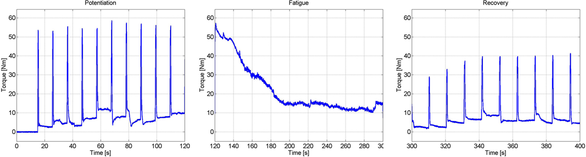
Figure 5. Results of the experiments to determine the parameters of the muscle fatigue parameters. These three plots show the torque measured during the potentiation, fatigue, and recovery segments of the procedure.
It was assumed that the muscle was fully rested at the beginning of the fatigue process. Therefore, the initial condition of the fatigue state was assumed as . Also, because the participant was being stimulated at the saturation amplitude for the duration of the fatigue procedure, the muscle activation variable was assumed to be 1 throughout the fatigue process (this is because the duration of the procedure is significantly longer than the muscle activation time constant that was previously determined). This approximation is necessary, as it allows us to measure the rate at which the muscle recovers without unnecessarily fatiguing the muscle. This procedure is identical to the potentiation procedure, where it can be observed that no noticeable muscle fatigue occurs. Using these assumptions the equation of the muscle fatigue dynamics (see equation (15)) can be reduced to whose solution, given the previously stated initial condition, is . A least-squares non-linear curve fitting algorithm was then used to solve for the parameters and that best fit the time response of the fatigue state to the normalized load cell measurement from the fatigue process. The normalized load cell data and the plot of the fatigue state that best fits the measured data are shown in Figure 6A. The resulting fit has an RMS error of 0.0373, and the parameters that were determined from this fit are and .
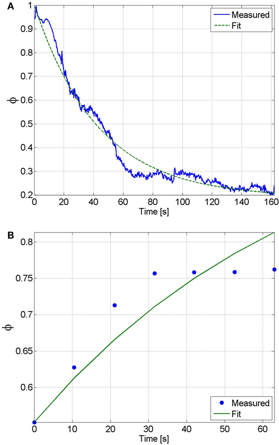
Figure 6. (A) The fatigue time constant and minimum fatigue states were determined by fitting the solution of the differential equation of the fatigue state to the normalized load cell data. From this fit, which has an RMS error of 0.0373, the fatigue time constant and minimum fatigue state were determined to be and , respectively. (B) The recovery time constant can be determined by fitting the solution of the differential equation of the fatigue state during recovery to the normalized load cell data. From this fit, which has an RMS error of 0.0031, the recovery time constant was determined to be .
During the recovery procedure, it was assumed that the pulses of stimulation were sufficiently short such that the muscle activation variable was essentially zero throughout the duration of the procedure. Therefore, the equation of the muscle fatigue dynamics can be reduced to , whose solution is , where is the initial condition that was measured from the first isometric contraction during the recovery procedure. The normalized load cell data and the plot of the fatigue state that best fits the measured data are shown in Figure 6B. The resulting fit has an RMS error of 0.0031, and the recovery time constant determined from the fit is . The estimated parameters of all of the participants are given in Table 1.
Table 1. Values of the estimated parameters and control gains used in the experiments for the right leg (RL) and left leg (LL) of each subject.
6. Experimental Results
The controller developed in equation (34) was validated through three sets of experiments on the right and left leg of three able-bodied subjects. The participants were seated in the leg extension machine, which is fitted with a CALT GHH100 rotary encoder (Shanghai Qiyi Electrical & Mechanical Equipment Co. Ltd.) to measure the knee angle, and were asked to remain completely relaxed and to avoid any volitional contractions that might influence the control. The first two sets of experiments used a desired sinusoidal trajectory with a minimum of 0° and a maximum of 45° and a period of 2 s. The third set of experiments tested the controllers’ ability to perform on a larger bandwidth of desired trajectories, 1-s time period and 4-s time period. The maximum amplitude of the 1-s time-period trajectory was reduced to 35°. The controller modulated the current amplitude while the pulse train’s frequency was fixed at 35 Hz with a pulse width of 400 μs. The 35 Hz pulse wave was used because it is within the optimal range for stimulating the muscle. It yields reduced fatigue in comparison to a higher frequency and produces a smoother motion compared with a lower frequency that tends to produce rippled knee motion (Riener et al., 1996). A pulse width can be chosen between the range of 100–500 μs. In this range, human skeletal muscle response to changes in stimulation amplitude (force–amplitude relationship) is highly predictable and thus was deemed appropriate for use in the current study. Because the new controller is a proportional-derivative (PD) type controller, tracking experiments using a PD controller were also conducted in the first two sets of experiments so that the performance of the new controller could be compared with a similar linear controller. In the third set of experiments, the controller was compared with a PD type controller augmented with a feedforward NN (Wang et al., 2013). The estimated control parameters and control gains for the fatigue compensation controller and the control gains for the PD controller from the first two sets of experiments are shown in Table 1, where Kp and Kd are the proportional and derivative gains of the PD controller, respectively. The control gains of the fatigue compensation controller (i.e., α, ks, and k) were introduced in equations (10), (25), and (34). The minimum muscle fatigue parameter, , for the right leg of Subject 3, which is approximately zero, indicates that when their quadriceps muscles are fully fatigued the stimulation will produce approximately no muscle force. The PD and FC controller gains given in Table 1 were determined experimentally using approximately 5–6 s long trials (per leg and per subject) before the 30 and 120 s long experiments. As no systematic tuning approach exists for the newly developed FC controller, the control gains were tuned through trial and error with the guidance of the knowledge of how each term in the controller affects the dynamics of the controlled system. Short duration trials were used to minimize the amount of muscle fatigue induced during tuning, and each subject was given 5 min after the tuning procedure to allow the participant to recover from any induced muscle fatigue before conducting the main experiments.
In the first set of experiments, after tuning the controller parameters, five 30-s long tracking experiment trials were performed on each leg of each participant for the FC and PD controllers. The root mean square (RMS) errors were computed for each trial, and then averaged over the five trials. The averaged RMS errors for the full duration of the experiments (0–30 s), the steady-state RMS (SSRMS) errors (ignores the first two periods of the desired trajectory), and the RMS of the current amplitude of the stimulation are shown in Table 2. Representative trials of the results of the fatigue compensation (FC) controller and the PD controller are shown in Figure 7. A Shapiro–Wilk test was used to determine if the RMS and SSRMS data were normal data sets. From the results of the Shapiro–Wilk test, it was concluded that the RMS and SSRMS PD controller data sets are not normal distributions. Therefore, a two-tailed Wilcoxon signed rank test with a 95% confidence level was used to determine if there was a difference between the FC and PD data sets. From the results of the Wilcoxon signed rank test,3 it was concluded that the FC and PD controllers are statistically different. Therefore, since the FC controller has a lower mean RMS and SSRMS error and because the data sets are significantly different it can be concluded that the FC controller yielded significantly better performance.
Table 2. Root mean square errors (RMS) for the full 30-s long trajectory tracking experiments and steady-state (4–30 s) RMS (SSRMS) errors averaged over five trials for the right leg (RL) and left leg (LL) of each subject for both the fatigue compensation (FC) and PD controllers.
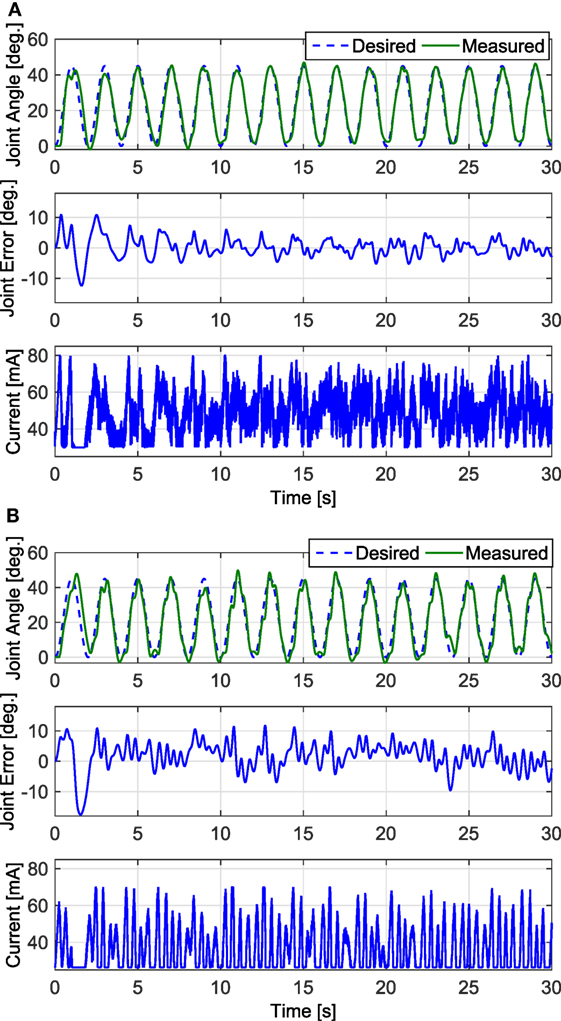
Figure 7. The trials that resulted in the lowest steady-state RMS errors for the fatigue compensation and PD controllers are shown in panels (A,B), respectively. The trial for the fatigue compensation controller was taken from one of Subject 1’s trials, which had a steady-state RMS error of 2.44°. The trial for the PD controller was taken from one of Subject 2’s trials, which had a steady-state RMS error of 4.23°.
In the second set of experiments, to determine how well the newly developed controller performed over long duration, where muscle fatigue should have a greater effect on performance, 2-min long tracking experiments were performed for one trial on each leg of each subject. A desired sinusoidal trajectory with a minimum of 0° and a maximum of 45° and a period of 2 s was used for the 2 min trials. Representative trials of the 2-min long experiments using the FC controller and the PD controller are shown in Figure 8, and the RMS errors computed from these trials are shown in Table 3. The RMS data sets were found to be not normally distributed, so a Wilcoxon signed rank test was used to conclude that there was a statistically significant difference between the FC and PD RMS data sets.4 Therefore, since the mean RMS error of the FC trials is lower than the mean RMS error of the PD trials it can be concluded that the FC controller also yielded significantly better performance over 2-min long trials.
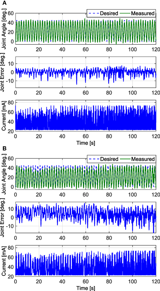
Figure 8. The 2-min long trials that resulted in the lowest RMS errors for the FC and PD controllers are shown in panels (A,B), respectively. Both trials were taken from the results of Subject 1’s left leg. The results of the FC controller in panel (A) had an RMS error of 3.24°, and the results of the PD controller in panel (B) had an RMS error of 6.96°.
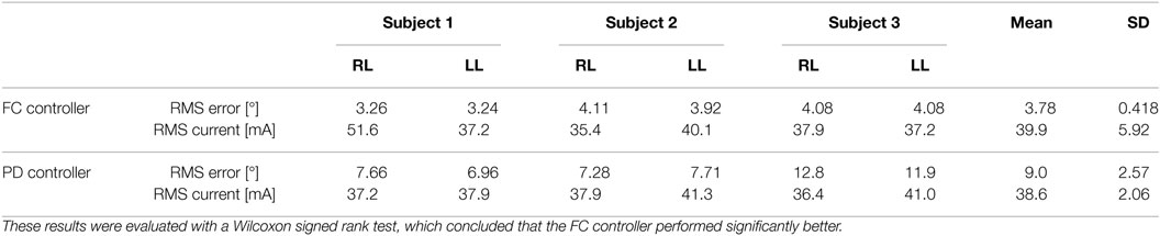
Table 3. RMS errors for 2-min long trials with PD and FC controllers for the right leg (RL) and left leg (LL) of each subject.
The estimated muscle fatigue state, obtained from the estimated models of muscle fatigue (see equation (15)), from the 2-min long trials are plotted in Figure 9 to illustrate the effect that each controller has on the estimate of muscle fatigue. Although the FC controller performed significantly better than the PD controller, it can be observed from Figure 9 that there is little difference in the muscle fatigue induced by both controllers. This was not the case for all subjects though as can be seen in Table 4, which shows the estimate of the fatigue states at the end of the 2-min long tracking trials. The fatigue state estimates were found to be not normally distributed, so a Wilcoxon signed rank test was used to conclude that there was no statistically significant difference between the two data sets.5 Therefore, because there is no statistical difference in the terminal fatigue estimate data it can be concluded that the FC controller does not cause any significant increase or decrease in muscle fatigue. Nevertheless, these values may not correlate with the actual fatigue and there is a caveat in making the conclusion that the two controllers might cause the same muscle fatigue. The main point is that the estimate show both controllers may be comparable in terms of inducing fatigue based on the estimated dynamics of fatigue. The estimated fatigue is an approximate quantifier of what is the capability of each controller in inducing fatigue, which based on Figure 9 and Table 4 comes out to be same.
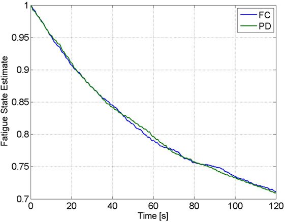
Figure 9. Estimate of the fatigue state, obtained from the estimated model of muscle fatigue, from the 2-min trials of Subject 1 for the FC and PD controllers.
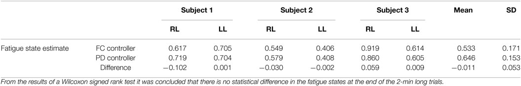
Table 4. The estimate of the fatigue states at the end of the 2-min long tracking trials for the right leg (RL) and left leg (LL) of each subject.
In the third set of experiments, to demonstrate the controllers’ ability to track trajectories with different frequencies, five 30 s trials were conducted on both legs of subject 2 for two more trajectories. The first trajectory, which is comparable with normal gait speeds, is twice as fast with a time period of 1 s and maximum amplitude of 35°. The second trajectory is half as slow with a time period of 4 s and maximum amplitude of 45°. In addition, to compare the FC controller to a similar class of adaptive controllers, a PD control with a feedforward NN was also tested in this set of experiments. The averaged RMS errors for the full duration of the experiments (0–30 s), the steady-state RMS (SSRMS) errors (ignores the first two periods of the desired trajectory), and the RMS of the current amplitude of the stimulation are shown in Table 5. Representative trials of the results of the fatigue compensation (FC) controller and the PD controller are shown in Figure 10. The subjects that were recruited for the previous set of experiments were unavailable for testing and more experiments were not performed for this set. Because this set of experiment was performed on only one subject, statistical tests are not included.
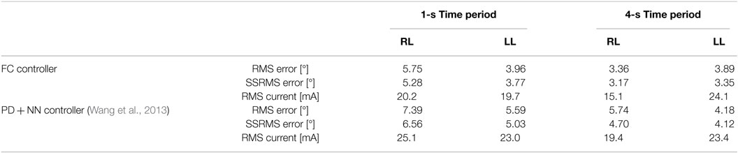
Table 5. Root mean square errors (RMS) for the full 30-s long trajectory tracking of 1 and 4 s time-period sinusoidal experiments and steady-state (2–30 and 8–30) RMS (SSRMS) errors averaged over five trials for the right leg (RL) and left leg (LL) of each subject for both the fatigue compensation (FC) and PD + NN controllers.
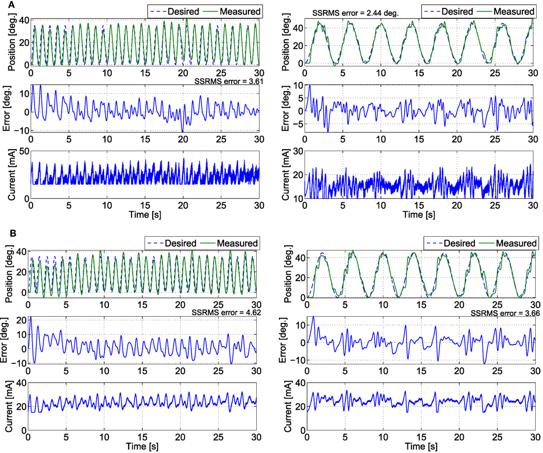
Figure 10. The trials that resulted in the lowest steady-state RMS errors for the (A) fatigue compensation and (B) PD + NN controllers for the (left) 1 s time-period trajectory and (right) 4 s time-period trajectory.
7. Discussion
Compared with our previous work, this work is a different control design because an integrator backstepping approach was employed to design an NMES controller that accounts for muscle fatigue and activation dynamics. The associated stability analysis is also different from the stability analyses of the RISE controllers (i.e., a different Lyapunov function is used). In our previous work with the RISE and RISE + NN controllers, the design approach only considered the second-order musculoskeletal dynamics. To account for muscle fatigue, an additional muscle activation dynamics needs to be added. This increases the order of the system from second order to third order. Our previous controllers RISE and RISE + NN are not designed for a third order system and their associated stability analyses for the 3rd order system may not be feasible. The ability of this controller to compensate for the effects of NMES-induced muscle fatigue is the main novelty of this developed controller, as no previously developed NMES controllers compensate for muscle fatigue. The control system presented in this article was originally developed in Sharma et al. (2009a). However, the previous work did not present a method for the implementation of this controller or any experimental results. This article concludes the work by presenting how the controller may be implemented through using estimated muscle parameters, procedures for estimating the required parameters, and experimental results that show the controller to have a statistically significant improvement over a PD controller. Also, given the developed control strategy and stability analysis, if a different first-order fatigue model (e.g., an EMG-based fatigue model) is available, it can be incorporated into the control design, which can provide a more accurate and real-time compensation of muscle fatigue.
To approximate the unknown model parameters, an NN-based feedforward approach was used. The NN design is based on an online update law and does not require a priori weight training. The estimates of the three-layer NN are updated by the laws given in equation (27). These laws allow the NN weights to be updated in real time, which are designed by using the Lyapunov control redesign process. According to Weierstrass–Stone theorem a three-layer NN can be used to approximate any continuous function up to a residual threshold, and hence, motivates the choice of a three-layer network. In three-layer NN, by increasing the number of hidden layer neurons (L), the approximation error can be reduced arbitrarily small, and the weights can be adjusted based on the adaptation law. For a two layer NN the basis function (hidden layer with activation functions) has to be selected carefully for practical implementations. This is not a problem with a three-layer NN because the input layer can be tuned to find an appropriate basis function. Moreover, the approximation error for a two layer NN is bounded from below on the order of , which implies that if the input dimension (n) is large, increasing L has no effect on reducing the approximation error (Lewis et al., 2002).
The work of Wang et al. (2013) presents the control development of an adaptive inverse optimal NMES controller. This work may seem similar to Wang et al.’s work as both papers used PD and neural network components; however, there are three major differences. First, the controller developed in Wang et al. is an optimal controller whose control objective is to minimize a user-specific cost functional, while the controller developed in this article is strictly error-based feedback control. Second, the controller developed in Wang et al. does not account for muscle fatigue, where as the controller developed in this paper models and compensates for the effects of muscle fatigue. Third, the control design approach and stability analyses of both papers are different because in Wang et al. an inverse optimal control approach was used to derive a PD + NN controller but in this current work a backstepping approach is used to derive a controller that uses PD + NN controller as a virtual control input (due to feedback type 3rd order dynamics), which leads to a controller that uses time derivatives of PD + NN controller.
The 30-s long and 2-min long trials illustrated that the developed controller performs significantly better than a PD controller. For the 30 s trials, the mean steady-state RMS errors for the PD controller and the FC controller were 6.73° and 3.93°, respectively. For the 2-min long trials the FC controller was shown to have a mean RMS error of 3.78°, while the PD controller was shown to have a mean RMS error of 9.04°. The 30-s long and 2-min long trials illustrated that the developed controller performs significantly better than a PD controller. For the 30 s trials, the mean steady-state RMS errors for the PD controller and the FC controller were 6.73° and 3.93°, respectively. For the 2-min long trials the FC controller was shown to have a mean RMS error of 3.78°, while the PD controller was shown to have a mean RMS error of 9.04°. The first two sets of experiments illustrated that the developed controller performs significantly better than a PD controller. For the first set of experiments, the mean steady-state RMS errors for the PD controller and the FC controller were 6.73° and 3.93°, respectively. For the second set of experiments, the FC controller was shown to have a mean RMS error of 3.78°, while the PD controller was shown to have a mean RMS error of 9.04°. A Wilcoxon signed rank test was used to show that the differences in performance were significant. The significant decrease in the performance of the PD controller for the 2-min long trials, compared with the 30-s long trials, indicated that the muscle fatigue does in fact cause a degradation in the control performance. However, for the newly developed FC controller there was no significant decrease in the performance of the controller for the 2-min long trials compared with the 30-s long trials. Therefore, it can be concluded that the newly developed FC controller is significantly more robust to the effects of muscle fatigue than a PD controller. Also, from the results of the third set of experiments, the FC controller is able to perform for slower and faster trajectories and fairs close to a PD + NN controller, which does not consider activation or fatigue dynamics. However, since only 1 subject was recruited for this set of experiment, the performance of the new controller with PD + NN controller lacks statistical significance. It should also be noted that the poor performance of the PD controller is also a result of its limitations as a linear controller. In other words, not only can the PD controller not compensate for the effects of muscle fatigue but it also cannot compensate for the other non-linearities of the system that are apparent in its dynamics in equation (8). A potential limitation of a PD controller is that high gain feedback is typically required to provide robustness to uncertain dynamics or unmodeled phenomena. High gain feedback can often result in large amplitude or high frequency control effort, which can lead to increased discomfort in people that are sensitive to stimulation intensity or lead to increased fatigue. The control gains can be adjusted to account for the level of noise in the feedback signal (i.e., which could result in high frequency stimulation) versus performance metrics and robustness. While various approaches have been documented for systematically adjusting the control gains for PD-like controllers (Åström et al., 1993; Killingsworth and Krstic, 2006), an empirical approach was used to obtain the results in this article. The results were obtained from the experiments performed on able-bodied subjects and any voluntary contributions from them may create a bias in the results. Therefore, the subjects were instructed to relax and not to interfere with FES and were unaware of the type of desired trajectory used. To completely ensure that the subjects would not interfere with the FES performance, EMG signals may be used to quantify any voluntary effort and thus remove any bias in the results.
Although the estimated muscle fatigue for the demonstrative trials were approximately equal for the two controllers, this was not true for all participants. From the results of the Wilcoxon signed rank test it was concluded that the developed controller does not cause any significant increase or decrease in muscle fatigue. However, it should be noted that this is an estimate of the muscle fatigue state and not the actual muscle fatigue state. Also, the controller is only compensating for the muscle fatigue to maintain the performance of the controller. The improved performance achieved by the FC controller was likely a result of the FC controller having a higher frequency response than the PD controller, as can be observed in Figures 7 and 8.
8. Conclusion
In this article, an NMES controller that incorporates the effects of muscle fatigue through an uncertain function of the activation dynamics was developed. The developed controller was shown to yield globally uniformly ultimately bounded tracking, provided that the sufficient conditions are met. The experimental results illustrate the feasibility of the controller to enable the lower leg to track a desired trajectory through stimulation of the quadriceps muscle. The focus of the current work was control development and analysis of the controller that incorporates muscle fatigue dynamics. The next step is to validate the new controller performance in a pathological case; e.g., stimulating muscles atrophied due to SCI. Especially, it will be interesting to see the controller’s performance when muscle is atrophied. The resulting control effectiveness of the muscle could be so low due to atrophy that not enough stimulation can be applied with safe limits to yield output. In other clinical populations, the user may be hyper sensitive to stimulation, limiting the amount that can be applied and also resulting in inefficient amount of stimulation. These issues and other implications from specific clinical populations would need to be considered in a more detailed clinical study, which is beyond the scope of this control development and analysis. The controller also needs to be tested for complex tasks that relate to activities of daily living. Therefore, our future work will focus on implementing the controller on clinical population and testing its performance during tasks such as walking elicited through FES.
Ethics Statement
Before any experimentation, approval from the Institutional Review Board at the University of Pittsburgh was obtained and each human subject was consented before participation.
Author Contributions
NS derived the back stepping control design for NMES control, conceptualized the experimental study, and wrote and edited the article. NK designed and performed parameter estimation experiments, validated the control design on human subjects, and wrote the experimental and discussion section. NA performed additional experiments and compared with a previous control design. WD advised in the control design and edited the article.
Conflict of Interest Statement
The authors declare that the research was conducted in the absence of any commercial or financial relationships that could be construed as a potential conflict of interest.
The reviewer, RN, and handling editor declared their shared affiliation.
Acknowledgments
The parts of the control development, analysis, and results presented in the article have been published in the dissertations of the authors, namely, by Sharma (2010) and Kirsch (2016).
Funding
This work was funded in part by the National Science Foundation award numbers 1462876 and 1511139 and the University of Pittsburgh’s Competitive Medical Research Fund and Central Research Development Fund.
Footnotes
- ^The controller may have a high frequency component due to the use of acceleration signals (xd contains the time derivative of the auxiliary signal, r). To remove the requirement for acceleration, the dynamic surface control (Alibeji et al., 2015) can be explored.
- ^Before any experimentation, approval from the Institutional Review Board at the University of Pittsburgh was obtained. The consent for the research participants was both informed and written.
- ^The critical test statistic value for a sample size of 30 and a 95% confidence level is 137, and the test statistic from the results of the Wilcoxon test was determined to be 4. Since the calculated test statistic is less than the critical test statistic it was concluded that the RMS and SSRMS data for the FC and PD controllers are significantly different.
- ^The critical test statistic value for a sample size of 6 and a 95% confidence level is 0, and the test statistic from the results of the Wilcoxon test was determined to be 0. Since the calculated test statistic is equal to the critical test statistic it was concluded that the RMS and SSRMS data for the FC and PD controllers are significantly different.
- ^The critical test statistic value for a sample size of 30 and a 95% confidence level is 0, and the test statistic from the results of the Wilcoxon test was determined to be 9. Since the calculated test statistic is greater than the critical test statistic it was concluded that there is no statistical difference between the two data sets.
References
Abbas, J. J., and Chizeck, H. J. (1991). Feedback control of coronal plane hip angle in paraplegic subjects using functional neuromuscular stimulation. IEEE Trans. Biomed. Eng. 38, 687–698. doi: 10.1109/10.83570
Ajoudani, A., and Erfanian, A. (2009). A neuro-sliding-mode control with adaptive modeling of uncertainty for control of movement in paralyzed limbs using functional electrical stimulation. IEEE Trans. Biomed. Eng. 56, 1771–1780. doi:10.1109/TBME.2009.2017030
Alibeji, N., Kirsch, N., and Sharma, N. (2015). “Dynamic surface control of neuromuscular electrical stimulation of a musculoskeletal system with activation dynamics and an input delay,” in American Control Conference (ACC) (Chicago, IL: IEEE), 631–636.
Asmussen, E. (1979). Muscle fatigue. Med. Sci. Sports. Exerc. 11, 313–321. doi:10.1249/00005768-197901140-00001
Åström, K. J., Hägglund, T., Hang, C. C., and Ho, W. K. (1993). Automatic tuning and adaptation for PID controllers – a survey. Control Eng. Prac. 1, 699–714. doi:10.1016/0967-0661(93)91394-C
Binder-Macleod, S. A., Dean, J. C., and Ding, J. (2002). Electrical stimulation factors in potentiation of human quadriceps femoris. Muscle Nerve 25, 271–279. doi:10.1002/mus.10027
Chang, G.-C., Lub, J.-J., Liao, G.-D., Lai, J.-S., Cheng, C.-K., Kuo, B.-L., et al. (1997). A neuro-control system for the knee joint position control with quadriceps stimulation. IEEE Trans. Rehabil. Eng. 5, 2–11. doi:10.1109/86.559344
Chen, Y.-L., Chen, W.-L., Hsiao, C.-C., Kuo, T.-S., and Lai, J.-S. (2005). Development of the FES system with neural network + PID controller for the stroke. Proc. IEEE Int. Symp. Circuits Syst. Kobe, 5, 5119–5121. doi:10.1109/ISCAS.2005.1465786
Cheng, T., Wang, Q., Kamalapurkar, R., Dinh, H., Bellman, M., and Dixon, W. (2016). Identification-based closed-loop NMES limb tracking with amplitude-modulated control input. IEEE Trans. Cybern. 46, 1679–1690. doi:10.1109/TCYB.2015.2453402
Ding, J., Wexler, A., and Binder-Macleod, S. (2002a). A predictive fatigue model. II. predicting the effect of resting times on fatigue. IEEE Trans. Rehabil. Eng. 10, 59–67. doi:10.1109/TNSRE.2002.1021587
Ding, J., Wexler, A., and Binder-Macleod, S. (2002b). A predictive fatigue model. I. predicting the effect of stimulation frequency and pattern on fatigue. IEEE Trans. Rehabil. Eng. 10, 48–58. doi:10.1109/TNSRE.2002.1021586
Downey, R., Bellman, M., Sharma, N., Wang, Q., Gregory, C., and Dixon, W. (2011). A novel modulation strategy to increase stimulation duration in neuromuscular electrical stimulation. Muscle Nerve 44, 382–387. doi:10.1002/mus.22058
Downey, R., Cheng, T., Bellman, M., and Dixon, W. (2015). Closed-loop asynchronous electrical stimulation prolongs functional movements in the lower body. IEEE Trans. Neural. Syst. Rehabil. Eng. 23, 1117–1127. doi:10.1109/TNSRE.2015.2427658
Ferrarin, M., Palazzo, F., Riener, R., and Quintern, J. (2001). Model-based control of FES-induced single joint movements. IEEE Trans. Neural Syst. Rehabil. Eng. 9, 245–257. doi:10.1109/7333.948452
Ferrarin, M., and Pedotti, A. (2000). The relationship between electrical stimulus and joint torque: a dynamic model. IEEE Trans. Rehabil. Eng. 8, 342–352. doi:10.1109/86.867876
Freeman, C. (2014). Upper limb electrical stimulation using input-output lineariztaion and iterative learning control. IEEE Trans. Control Syst. Technol. 23, 1546–1554. doi:10.1109/TCST.2014.2363412
Freeman, C. T., Hughes, A.-M., Burridge, J. H., Chappell, P. H., Lewin, P. L., and Rogers, E. (2009). A model of the upper extremity using FES for stroke rehabilitation. J. Biomech. Eng. 131, 031011. doi:10.1115/1.3005332
Giat, Y., Mizrahi, J., and Levy, M. (1993). A musculotendon model of the fatigue profiles of paralyzed quadriceps muscle under FES. IEEE Trans. Biomed. Eng. 40, 664–674. doi:10.1109/10.237696
Giuffrida, J. P., and Crago, P. E. (2005). Functional restoration of elbow extension after spinal-cord injury using a neural network-based synergistic FES controller. IEEE Trans. Neural Syst. Rehabil. Eng. 13, 147–152. doi:10.1109/TNSRE.2005.847375
Happee, R. (1994). Inverse dynamic optimization including muscular dynamics, a new simulation method applied to goal directed movements. J. Biomech. 27, 953–960. doi:10.1016/0021-9290(94)91277-7
Hatze, H. (1977). A myocybernetic control model of skeletal muscle. Biol. Cybern. 25, 103–119. doi:10.1007/BF00337268
Jezernik, S., Wassink, R. G., and Keller, T. (2004). Sliding mode closed-loop control of FES controlling the shank movement. IEEE Trans. Biomed. Eng 51, 263–272. doi:10.1109/TBME.2003.820393
Killingsworth, N. J., and Krstic, M. (2006). PID tuning using extremum seeking: online, model-free performance optimization. IEEE Contr. Syst. Mag. 26, 70–79. doi:10.1109/MCS.2006.1580155
Kirsch, N. A. (2016). Control Methods for Compensation and Inhibition of Muscle Fatigue in Neuroprosthetic Devices. PhD thesis, University of Pittsburgh.
Klauer, C., Schauer, T., Reichenfelser, W., Karner, J., Zwicker, S., Gandolla, M., et al. (2014). Feedback control of arm movements using neuro-muscular electrical stimulation (NMES) combined with a lockable, passive exoskeleton for gravity compensation. Front. Neurosci. 8:262. doi:10.3389/fnins.2014.00262
Kordylewski, H., and Graupe, D. (2001). Control of neuromuscular stimulation for ambulation by complete paraplegics via artificial neural networks. Neurol. Res. 23, 472–481. doi:10.1179/016164101101198866
Krstic, M., Kanellakopoulos, I., and Kokotovic, P. V. (1995). Nonlinear and Adaptive Control Design. New York, NY: Wiley.
Lan, N., Crago, P. E., and Chizeck, H. J. (1991a). Control of end-point forces of a multijoint limb by functional neuromuscular stimulation. IEEE Trans. Biomed. Eng. 38, 953–965. doi:10.1109/10.88441
Lan, N., Crago, P. E., and Chizeck, H. J. (1991b). Feedback control methods for task regulation by electrical stimulation of muscles. IEEE Trans. Biomed. Eng. 38, 1213–1223. doi:10.1109/10.137287
Levy, M., Mizrahi, J., and Susak, Z. (1990). Recruitment, force and fatigue characteristics of quadriceps muscles of paraplegics, isometrically activated by surface FES. J. Biomed. Eng. 12, 150–156. doi:10.1016/0141-5425(90)90136-B
Lewis, F. L. (1996). Neural network control of robot manipulators. IEEE Expert 11, 64–75. doi:10.1109/64.506755
Lewis, F. L., Selmic, R., and Campos, J. (2002). Neuro-Fuzzy Control of Industrial Systems with Actuator Nonlinearities. Philadelphia, PA, USA: Society for Industrial and Applied Mathematics.
Lynch, C., and Popovic, M. (2012). A comparison of closed-loop control algorithms for regulating electrically stimulated knee movements in individuals with spinal cord injury. IEEE Trans. Neural Syst. Rehabil. Eng. 20, 539–548. doi:10.1109/TNSRE.2012.2185065
Maladen, R., Perumal, R., Wexler, A., and Binder-Macleod, S. (2007). Effects of activation pattern on nonisometric human skeletal muscle performance. J. Appl. Physiol. 102, 1985–1991. doi:10.1152/japplphysiol.00729.2006
Riener, R., and Fuhr, T. (1998). Patient-driven control of FES-supported standing up: a simulation study. IEEE Trans. Rehabil. Eng. 6, 113–124. doi:10.1109/86.681177
Riener, R., Quintern, J., and Schmidt, G. (1996). Biomechanical model of the human knee evaluated by neuromuscular stimulation. J. Biomech. 29, 1157–1167. doi:10.1016/0021-9290(96)00012-7
Russ, D., Vandenborne, K., and Binder-Macleod, S. (2002). Factors in fatigue during intermittent electrical stimulation of human skeletal muscle. J. Appl. Physiol. 93, 469–478. doi:10.1152/japplphysiol.01010.2001
Schauer, T., Negard, N. O., Previdi, F., Hunt, K. J., Fraser, M. H., Ferchland, E., et al. (2005). Online identification and nonlinear control of the electrically stimulated quadriceps muscle. Control Eng. Pract. 13, 1207–1219. doi:10.1016/j.conengprac.2004.10.006
Sepulveda, F. (2003). “Artificial neural network techniques in human mobility rehabilitation,” in Computational Methods in Biophysics, Biomaterials, Biotechnology and Medical Systems, ed. C. T. Leondes (Boston, MA: Springer), 313–348.
Sharma, N. (2010). Lyapunov-Based Control Method for Neuromuscular Electrical Stimulation. PhD thesis, University of Florida.
Sharma, N., Gregory, C., and Dixon, W. E. (2011). Predictor-based compensation for electromechanical delay during neuromuscular electrical stimulation. IEEE Trans. Neural Syst. Rehabil. Eng. 19, 601–611. doi:10.1109/TNSRE.2011.2166405
Sharma, N., Gregory, C. M., Johnson, M., and Dixon, W. E. (2012). Closed-loop neural network-based NMES control for human limb tracking. IEEE Trans. Control Syst. Technol. 20, 712–725. doi:10.1109/TCST.2011.2125792
Sharma, N., Patre, P., Gregory, C., and Dixon, W. (2009a). “Nonlinear control of NMES: incorporating fatigue and calcium dynamics,” in Proceedings of ASME Dynamic Systems and Control Conference (Hollywood, CA: ASME).
Sharma, N., Stegath, K., Gregory, C. M., and Dixon, W. E. (2009b). Nonlinear neuromuscular electrical stimulation tracking control of a human limb. IEEE Trans. Neural Syst. Rehabil. Eng. 17, 576–584. doi:10.1109/TNSRE.2009.2023294
Tong, K. Y., and Granat, M. H. (1999). Gait-control system for functional electrical stimulation using neural networks. Med. Biol. Eng. Comput. 37, 35–41. doi:10.1007/BF02513359
Wang, Q., Sharma, N., Johnson, M., Gregory, C. M., and Dixon, W. E. (2013). Adaptive inverse optimal neuromuscular electrical stimulation. IEEE Trans. Cybern. 43, 1710. doi:10.1109/TSMCB.2012.2228259
Zajac, F. (1989). Muscle and tendon: properties, models, scaling, and application to biomechanics and motor control. Crit. Rev. Biomed. Eng. 17, 359–411.
Zhang, D., and Zhu, K. (2004). Simulation study of FES-assisted standing up with neural network control. Proceedings of IEEE EMBS, San Francisco, CA, 7, 4877–4880. doi:10.1109/IEMBS.2004.1404349
Appendix
Let V ∈ ℝ denote a continuously differentiable, non-negative, radially unbounded function defined as
By using equation (13) and typical NN properties (Lewis et al., 2002), V can be upper and lower bounded as
where λ1,λ2,θ ∈ ℝ+ are known positive constants, and X ∈ ℝ3 is defined as
Taking the time derivative of equation (A1), utilizing equations (10) and (31), the definition of ks, and canceling similar terms yields
Using equations (14), (27), and (32), the expression in equation (A4) can be upper bounded as
Assuming that equation (36) is satisfied, and substituting equation (35) into equation (A5), results in
Completing the squares for the bracketed term in equation (A6), and further bounding the expression yields
The inequality in equation (A2) can be used to rewrite equation (A7) as
where δ ∈ ℝ+ is a positive constant defined as
and β ∈ ℝ is defined as
The linear differential inequality in equation (A8) can be solved as
Based on equations (A2) and (A9), it can be derived that
which can be used, along with equation (A3), to show that the error can be bounded as
where , , and .
Provided the sufficient condition in equation (38) is satisfied, the expressions in equations (A10) and (A11) indicate that e, r, ex, . Given that e, r, qd, , equations (9) and (10) indicate that q, . Since , the boundedness of the ideal weights (Lewis et al., 2002) can be used to conclude that . Based on equation (5), it can be shown that . Given that , e, r, q, , , the NN input vector βy ∈ Λ∞ from equation (22). Since ex, , equation (29) can be used to show that xd ∈ Λ∞. Given that r, , , , equations (25) and (26) indicate that , . Since e, r, , , , , equations (31) and (32) indicate that . As r, y, , the update laws . Since , it can be shown that . Given that the , , , r, , it can be shown that . Because , it can be concluded that the stimulation control input v is bounded.
Keywords: integrator backstepping, neural networks, muscle fatigue, Lyapunov stability, neuromuscular electrical stimulation
Citation: Sharma N, Kirsch NA, Alibeji NA and Dixon WE (2017) A Non-Linear Control Method to Compensate for Muscle Fatigue during Neuromuscular Electrical Stimulation. Front. Robot. AI 4:68. doi: 10.3389/frobt.2017.00068
Received: 15 August 2017; Accepted: 24 November 2017;
Published: 22 December 2017
Edited by:
Ramana Vinjamuri, Stevens Institute of Technology, United StatesReviewed by:
Raviraj Nataraj, Stevens Institute of Technology, United StatesMarco Capogrosso, University of Fribourg, Switzerland
Copyright: © 2017 Sharma, Kirsch, Alibeji and Dixon. This is an open-access article distributed under the terms of the Creative Commons Attribution License (CC BY). The use, distribution or reproduction in other forums is permitted, provided the original author(s) or licensor are credited and that the original publication in this journal is cited, in accordance with accepted academic practice. No use, distribution or reproduction is permitted which does not comply with these terms.
*Correspondence: Nitin Sharma, bmlzNjJAcGl0dC5lZHU=