From simulation to reality: experimental analysis of a quantum entanglement simulation with slime molds (Physarum polycephalum) as bioelectronic components

This study investigates whether it is possible to simulate quantum entanglement with theoretical memristor models, physical memristors (from Knowm Inc.) and slime molds Physarum polycephalum as bioelectric components. While the simulation with theoretical memristor models has been demonstrated in the literature, real-world experiments with electric and bioelectric components had not been done so far. Our analysis focused on identifying hysteresis curves in the voltage-current (I-V) relationship, a characteristic signature of memristive devices. Although the physical memristor produced I-V diagrams that resembled more or less hysteresis curves, the small parasitic capacitance introduced significant problems for the planned entanglement simulation. In case of the slime molds, and unlike what was reported in the literature, the I-V diagrams did not produce a memristive behavior and thus could not be used to simulate quantum entanglement. Finally, we designed replacement circuits for the slime mold and suggested alternative uses of this bioelectric component.

1 Introduction

This paper focuses on slime mold-based bioelectronics and an attempt to simulate quantum computing with bioelectric components. The synthesis of biology, electronics, and quantum mechanics explores the convergence of disparate fields, offering insights of the challenges of bioelectronics and quantum computational paradigms. Through this interdisciplinary lens, we uncover the difficulties at the intersection of nature-inspired algorithms and quantum computing theory.

We started with the following assumptions: i) slime molds can (sometimes) act as memristors, ii) memristors can be used to simulate quantum circuits. Based on these assumptions, we wanted to experimentally find out if slime molds could be used to simulate quantum circuits classically.

In the first part of the manuscript, we introduce the memristor as a relatively new electronic component, the slime mold Physarum polycephalum as an experimental organism, and a summary of how quantum entanglement could be simulated with memristors. In the results section, we present the outcomes of our experiments, examine the electric characteristics of slime molds as potential biomemristors, and finally, discuss alternative bioelectric applications for the slime mold.

1.1 Memristors

A memristor is a non-linear electronic device that is a resistor with a memory, hence the name memristor. It is the fourth fundamental two-terminal circuit element. The other three are the resistor, defined by a relationship between voltage (v) and current (i); the inductor, defined by a relationship between flux $(\varphi )$ and current (i); and the capacitor, defined by a relationship between charge (q) and voltage (v). The memristor is characterized by a relationship between flux $(\varphi )$ and charge (q) (Chua, 2018).

While the memristor was theoretically predicted in the early 1970s (Chua, 1971), it was only in 2008 when a team of scientists from Hewlett-Packard labs built the first operational monolithic memristor made by sandwiching a thin film of titanium dioxide between platinum electrodes (Strukov et al., 2008). In addition to providing the physical operating mechanism (Strukov et al., 2008), they also showed a pinched hysteresis loop (which looks like a tilted figure eight), which is the hallmark of all memristors. In contrast to a regular resistor, the memristor has a dynamic relationship between current (I) and voltage (V), which means that the electrical resistance (R = U/I) changes because of past voltages. Following the invention of the physical memristor, additional two-terminal circuit elements with memory were described, namely the memcapacitor and the meminductor (Di Ventra et al., 2009). Memfractors or fractional memory elements have interpolated characteristics between a memcapacitor, a memristor, and a meminductor (Abdelouahab et al., 2014).

Memristive devices could potentially be an alternative for CMOS-based logic computation as they do not require a separate data storage and computation (von Neumann) architecture (Luo et al., 2020; Lehtonen et al., 2010; Chattopadhyay and Rakosi, 2011).

They can carry out fundamental Boolean logic operations (Lehtonen et al., 2010) where the same devices serve simultaneously as logic gates and memory that use resistance (instead of voltage or charge) as the physical state variable (Ielmini and Milo, 2017; Borghetti et al., 2010). Studies in recent years have shown that we can expect viable memristor-based non-von Neumann hardware solutions for deep neural networks, artificial intelligence and edge computing (Yao et al., 2020; Jebali et al., 2024; Aguirre et al., 2024; Huang et al., 2024).

Sparse coding with memristor networks is of broad interest for applications in signal processing, computer vision, object recognition and neurobiology (Sheridan et al., 2017). The connection between memristors and neurobiology is of particular interest. Memristors have for example been deployed to create artificial neurons and carry out neuromorphic computing (Snider, 2003; Snider et al., 2011; Park et al., 2022).

The learning behavior of slime molds (Physarum polycephalum) has also been modeled with memristors (Pershin et al., 2009).

1.2 Slime mold Physarum polycephalum as an experimental organism and possible memristor

Physarum polycephalum is a slime mold found in cool, moist and dark environments, for example, in the woods, on decaying leaves and tree bark (Figure 1). It is a single eukaryotic cell with many heads; hence the term ‘polycephalum’. It is typically yellow and visible to the naked eye. This organism feeds through a process called phagocytosis. It coats its food in enzymes, allowing specific nutrients to be ingested, leaving behind a mass of unwanted material. In the laboratory, oat flakes are used to feed it (Figure 1).

Figure 1

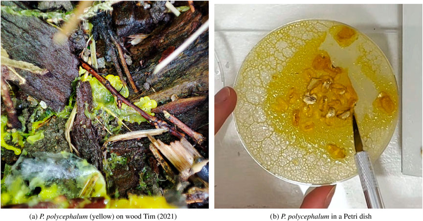
Figure 1. Physarum polycephalum on decaying a tree bark (a). Physarum polycephalum culture in a Petri dish feeding on oat flakes (b).

Physarum polycephalum exhibits a complex life cycle, but the point of interest here is its plasmodium stage, when the organism actively searches for food. As it does so, it grows a network of protoplasmic tubes that rhythmically contract and expand, producing shuttle streaming of its internal fluid.

The organism is straightforward to culture in Petri dishes (Figure 1) and it is relatively easy to prompt it to grow specific topologies of protoplasmic tubes by placing food and repellents (e.g. salt) strategically on the dish. The ability to manipulate its growth patterns has underpinned the early stages of research into building Physarum polycephalum-based machines to realize tasks deemed as computational: e.g., the organism was prompted to find the shortest path to a target destination through a maze (Adamatzky, 2015b).

The focus of our research is the electrical behavior of Physarum polycephalum. Its intracellular activity produces fluctuating levels of electrical potential. Typically, this is in the range of ± 50 mV, displaying oscillations at periods between 50s and 200s, with amplitudes ranging from 5 mV to 40 mV (Kishimoto, 1958; Adamatzky and Jones, 2011; Adamatzky, 2014; Boussard et al., 2021; Wohlfarth-Bottermann, 1979). Interestingly, electrical current can be relayed through its protoplasmic tube, and this prompts it to behave like an electronic component.

Several research papers have found that Physarum polycephalum has the ability to solve mazes (Nakagaki et al., 2000), remember and anticipate events (Saigusa et al., 2008), actively balance its diet (Bonner, 2010) and grow in a way that matches efficient road networks (Adamatzky and Jones, 2010). Researchers in the field of unconventional computing are quite fascinated with the ways P. polycephalum can be used in electronics and computing, one review paper lists 25 different applications (Adamatzky, 2015b).

In the literature, slime molds have also been reported to sometimes have memristive properties (Gale et al., 2016). Gale et al. wrote, for example, that they tested 11 slime molds of which “2 exhibited good memristance curves, the other 9 exhibited open curves” (Gale et al., 2014). Other studies reported no memristive behavior in slime mold (Schmidt et al., 2025).

1.3 Simulating quantum circuits with memristors

For the development of quantum computing, considering its associated costs, limited availability, and high error rates, not every experiment can or should run on a quantum computer. This is why quantum simulators and classical simulators of quantum computers are essential parts of the quantum computing development efforts. The Gottesman-Knill theorem (Aaronson and Gottesman, 2004) states that a quantum circuit consisting solely of CNOT, Hadamard, and phase gates can be classically efficiently simulated. Therefore, in addition to the quantum hardware that can simulate quantum computers, there is a wide range of quantum circuits that can run operations efficiently on classical hardware without the need for a quantum hardware. Below, a range of available quantum simulators and proposals are covered.

Memristors were reported to efficiently simulate certain quantum circuits containing Hadamard and CNOT gates, which combined can be used to create entanglement (Karafyllidis et al., 2018; Fyrigos et al., 2018; Karafyllidis et al., 2019). According to these authors, memristors can be used for Qubit state representation and simulating quantum computers. Here we provide a very short summary of how this is done, see the original papers for more detailed explanations.

Since the qubit is the elementary module of a quantum computing system (Fyrigos et al., 2018) it has been suggested that the first step towards a memristor-based one is to model the representation of a qubit by memristors. They suggested a model where the state of the qubit was mapped to a 3-D memristance space. Starting out with the representation of a qubit $|q\rangle$ that is described in Equation 1 by the superposition of a 0 and 1 state:

$|\mathbf{q}\rangle =a|0\rangle +b|1\rangle (1)$

The quantum state $|\mathbf{q}\rangle =a|0\rangle +b|1\rangle$ (1), where $a,b\in \mathbb{C}$, has certain probabilities $P(|\mathbf{q}\rangle =|0\rangle )=|a{|}^2$ and $P(|\mathbf{q}\rangle =|1\rangle )=|b{|}^2$, satisfying the normalization condition:

$|a{|}^2+|b{|}^2=1(2)$

Using the Bloch sphere and its coordinate system, Equation 2 can be represented as Equation 3:

$|\mathbf{q}\rangle =\cos \frac{\theta }{2}|0\rangle +e^{i\phi }\sin \frac{\theta }{2}|1\rangle (3)$

where $\theta$, $\phi \in \mathbb{R}$. We can further reduce the complexity of the formula using Euler’s identity, leading to Equation 4:

$|\mathbf{q}\rangle =\cos \frac{\theta }{2}|0\rangle +\cos \phi \sin \frac{\theta }{2}|1\rangle +i\sin \phi \sin \frac{\theta }{2}|1\rangle (4)$

Where we now have mapped three factors of a “qubit’s basis state (one for the real part of each state and one for the imaginary part of $|1\rangle$) to the resistance values of a set of three memristor devices $M_j$ for $j=\mathrm{1,2,3}$ (3D Memristance Space). More specifically, the time evolution of $V_j$, described below, is applied to the corresponding $M_j$ and drives its time evolution in accordance with the qubit representation equations. The applied voltages to memristors as functions of time are:” (Fyrigos et al., 2018).

$V_j\left(t\right)=\left\{\begin{array}{cc}\cos \frac{\theta \left(t\right)}{2}\hfill & \text{for\hspace{0.17em}}j=1\hfill \\ \cos \varphi \left(t\right)\sin \frac{\theta \left(t\right)}{2}\hfill & \text{for\hspace{0.17em}}j=2\hfill \\ \sin \varphi \left(t\right)\sin \frac{\theta \left(t\right)}{2}\hfill & \text{for\hspace{0.17em}}j=3\hfill \end{array}\right.(5)$

A group of three memristors can be used to represent the qubit state, which, using Equation 5, becomes Equation 6:

$|\mathbf{q}\rangle =V_1\left(t\right)|0\rangle +V_2\left(t\right)|1\rangle +i{V}_3\left(t\right)|1\rangle (6)$

In other words, each line in Equation 5 represents one dimension in a 3D space that represents a qubit Bloch sphere. For each dimension one memristor is needed, so we need three memristors to simulate one qubit, and the simulation requires that each memristor is presented with the voltage input specified in Equation 5 (see corresponding Figure 4 in the Results section). For further details on the mathematics behind this, see Karafyllidis et al. (2019).

1.4 Aim of the study

Here we draw on recent work that suggests that: A) slime molds (sometimes) behave like memristors. B) (simulated) memristors can be used to simulate quantum entanglement. When A and B are true, it follows that slime molds can be used to simulate quantum entanglement and thus a key feature of quantum computers.

The first aim of the study was to examine the claim that slime molds are indeed behaving like memristors, as there seem to be conflicting statements in the literature, and if they do, if they could simulate a quantum entanglement?

The second aim was to create a replacement circuit to describe the electric behavior of slime molds and discuss other potential bioelectric uses of P. polycephalum.

2 Methodology

2.1 Cultivation of Physarum polycephalum

In the cultivation of P. polycephalum for our experiments, we initiated the process by establishing a robust stock culture in 55 mm Petri dishes. Subsequently, new cultures were systematically developed in 50 mL conical centrifuge tubes. The cultures in the Petri-dishes and the tubes were sealed in sterile polypropylene bags with 0.2 $\mu$ filter disc until usage. The centrifuge tubes were chosen for their practicality and ease of handling in our experimental setup. After a period of 4 days, in an average, the plasmodium cultures were ready for the measuring experiments. The slime molds were stored in an opaque case at room temperature (Schmidt et al., 2025).

2.1.1 Culture setup

To provide the necessary humidity and nutrients for growth, each tube was filled with a nutrient-free agar medium, sterilized oat flakes placed on top of it. The oat flakes were sterilized for 30 min at 120 °C in a Lacor 22 L pressure cooker. The design involved the inclusion of a 3 mm aperture positioned at the 32.5 mL markings within each centrifuge tube. This orifice functioned as a designated site for the integration of an electro-conductive collar, in parts modeled after the design of Braund and Miranda (2017).

2.1.2 Electro-conductive collar design and 3D printing

The electro-conductive collar, with an outer diameter of 4 mm and an inner diameter of 1.5 mm, was designed and 3D printed using a Prusa MK3 printer with the RepRapper Conductive PLA.

2.1.3 PVC tube connection setup

The experimental setup further involved the connection of two centrifuge tubes through a PVC tube with a length of 15 mm, to facilitate the growth of the slime mold through the PVC tube, connecting the two electro-conductive collars (adapters). These collars were linked to electrodes, allowing for the application of electric currents through the plasmodium, see Figure 2.

Figure 2

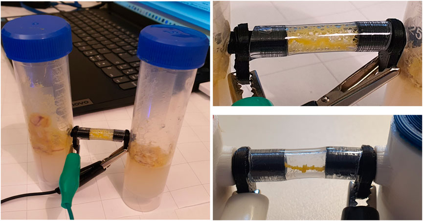
Figure 2. The slime mold measurements in the test tube set up. Overall view and details of the tube with the black electric conductive rings.

2.2 Electric measurements of Physarum polycephalum

2.2.1 Electrode connection and current measurement

To assess the response of P. polycephalum to electric currents, we utilized a Rigol DG1022 function generator to generate the currents under investigation. Simultaneous measurement of both volts and amperes became a crucial aspect of our methodology. This approach was deemed indispensable because of the sensitivity of the experimental system; even minimal imprecision in the alignment of measuring points could result in misleading data, potentially yielding erroneous hysteresis curves (Schmidt et al., 2025). The slime mold was seeded in one of the two vertical containers, with food placed in the other one. The slime grew to the other container via the horizontal transparent tube that was connected to the black conductive contacts where measurements were carried out. In the beginning the slime mold grew like a net (see Figure 2 upper right) but after some days the different strands consolidated to a single tube (see Figure 2 lower right).

2.2.2 Measurement instrumentation

For the simultaneous measurement/calculation of volts and amperes, we employed the Diligent Analog Discovery 3 in conjunction with a measuring circuit fitted onto a breadboard. Analog Discovery 3 allows for the synchronous measurement of 2 separate Voltage channels. In addition to measuring the applied Voltage from the Rigol DG1022 function generator, the Ampere values were calculated by measuring the Voltage at a serial resistance measured at 150 K Ω, using Ohm’s law we calculated I=U/R. This setup allowed us to precisely capture and record the electrical responses of P. polycephalum during the experiments, using the Digilent Waveform3 software as a logging device. Additionally, we conducted a second A control measurement using a Rigol DM3056e digital multimeter (which had a different measurement timing and was only used to control the resulting values of the Diligent Analog Discovery 3) (Schmidt et al., 2025). The Analog Discovery 3 was regularly calibrated according to the manufacturer’s calibration guidelines (Arduino, 2023). These calibration procedures ensured stable and reproducible results throughout the experimental period.

2.2.3 Environmental conditions and slime mold viability

We report laboratory conditions based on a few separate measurements. These measurements indicated an average room temperature of 23,6 °C and an average relative humidity of 44,5%, measured using a DHT22 sensor connected to an Arduino Uno R4 (Arduino, 2023; SparkFun, 2010).

Slime mold viability was not used as an exclusion criterion during the experiments; we measured all available cultures, including those showing signs of dormancy (sclerotia formation) or reduced activity. However, for a dedicated control group measurement, we used cultures that had been cultivated on 3 April 2024 and re-measured on 19 August 2025 (503 days), by which time they were most likely dead, as indicated by their sclerotic appearance.

The study consisted of two main segments of measurements that included slime mold cultures. The main measurements, conducted from 25 January 2024, to 3 April 2024, and included 289 observations across 38 distinct slime mold cultures. Prior to this, the test measurements occurred over 14 days between 2 June 2023, and 22 December 2023, involving 195 observations from over 20 different cultures, including 44 controls such as office plants, cacti, and dummy resistors. Additional 23 comparative measurements were done from August 19-20, 2025, of which 4 were with slime molds, resulting in a total of 293 slime mold measurements. The living slime mold cultures ranged in age from 4 to 25 days, providing a fairly large dataset for analysis. To assess baseline electrical behavior of non-biological and non-Physarum samples and to identify possible setup artifacts, we performed a set of control and comparison measurements. These included distilled water (VDE 0510 compliant), Viennese tap water, and a 1% NaCl solution prepared from 100 g distilled water (VDE 0510) and 1 g NaCl. We also tested an empty tube from our setup (PVC tube with 3D-printed adapters made from RepRapper conductive PLA) as well as the same tube filled with the 1% NaCl solution.

Additional biological controls included a Trichocereus macrogonus var. Pachanoi cactus, a basil plant (Ocimum basilicum), hard cheese and vegan coconut yoghurt. These measurements were acquired with the same instrumentation and wiring as used for the P. polycephalum experiments, employing identical sinus waveforms and logging procedures, allowing direct comparison of signal levels and potential hysteresis-like artifacts across biological, non-biological, and hardware-only baselines. See Table 1 and for more details, Table 2.

Table 1

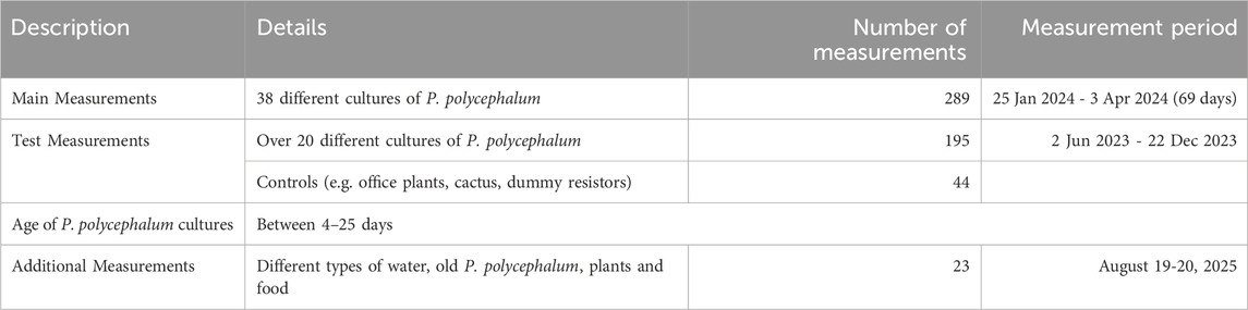
Table 1. Summary of electric measurements with Physarum polycephalum.

Table 2

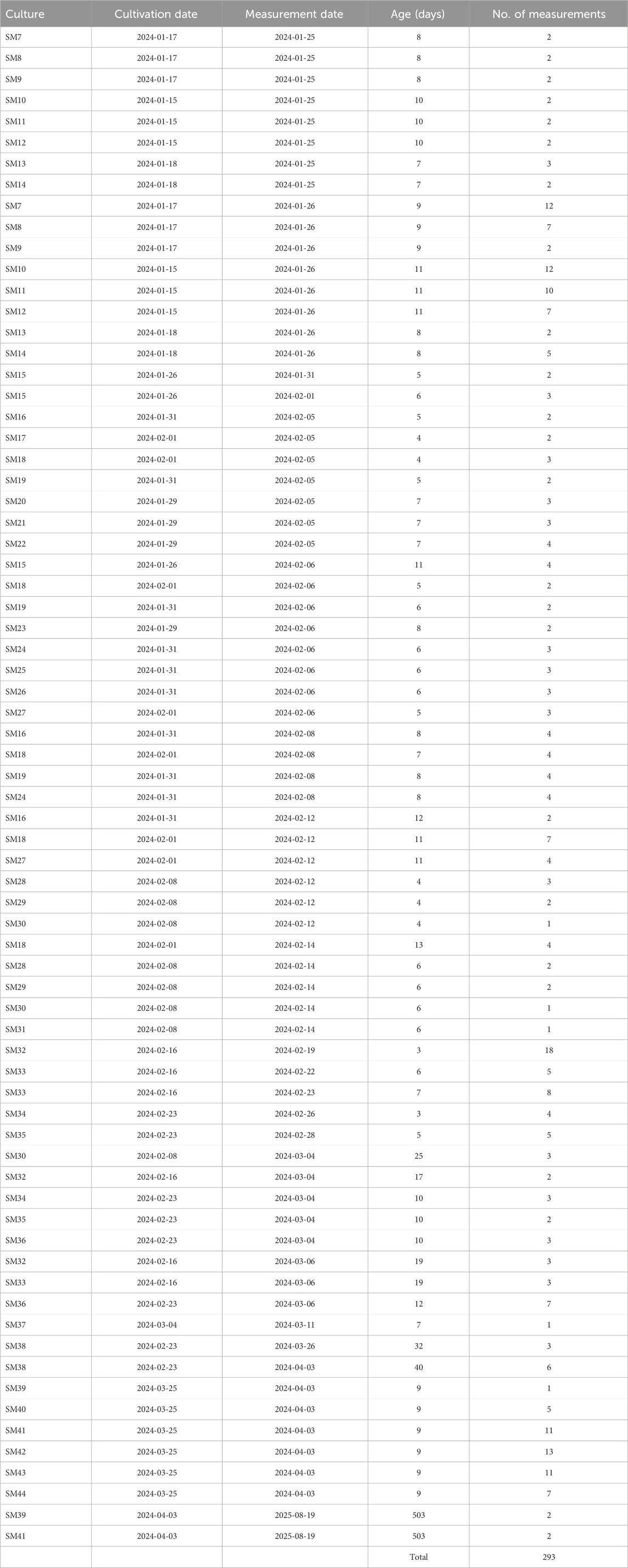
Table 2. Details of electric slime mold measurements.

The datasets generated and analyzed during the current study are available in the Mendeley repository: https://data.mendeley.com/datasets/ghm9gvwwvb/1.

2.3 Electric measurements of physical memristor

As a comparison, we conducted the experiments not only with the slime molds but also with a real physical memristor, the Knowm Inc. 1 × 16 array memristor chip.

In our investigation, we used the Memristor Discovery platform, consisting of the Memristor Discovery board v.2 integrated with the Diligent Digilent Analog Discovery 3 for data collection and analyses.

After connecting the Knowm 1 × 16 array memristor chip onto the Memristor Discovery board we conducted standard experiments provided by the Memristor Discovery software to familiarize ourselves with the setup and operation of the system.

The open-source nature and available documentation of the Memristor Discovery software, allowed tinkering the experimental parameters to match those used in our previous slime mold experiments, by changing the code of the software in the Eclipse, version 4.30, development environment. Specifically, we adjusted the waveform characteristics to obtain the three different input signals shown in 5.

We documented the graphical outputs using the save function to record pictures of the behavior of the memristors using our parameters. Additionally, the Memristor Discovery software allowed the export of numerical data in the form of. csv spreadsheets which were used for further analysis.

2.4 Software based electric circuit simulation

Additionally, we conducted experiments using software simulations of memristors using the LTspice software. This simulation environment enabled the incorporation of various memristor models into its library, allowing modeling different memristor characteristics. Within the LTspice software, MacOs version 17.2.2, we constructed a virtual version of our experimental circuit, mirroring the setup utilized in our slime mold experiments. This virtual representation allowed us to simulate the behavior of memristors under conditions like those encountered in our physical experiments. We generated the same three input signals as in the previous experiments using. pwl files. We conducted simulations to observe the response of the virtual memristors, to compare the electrical behavior of memristors and the physiological responses of slime molds. Documentation was retrieved using the data export function within the LTspice software (Schmidt et al., 2025).

2.5 Data processing

2.5.1 Data inclusion and file parsing

CSV files were ingested from the experimental repository. We analyzed only files that met two criteria recorded in an external metadata table (Excel): (i) the waveform was a sinus, and (ii) the total length of the recorded measurement was $<1000$ seconds to exclude measurements that did not complete a full cycle. For each selected CSV, we read the voltage, current and time columns. Non-data and comment lines were ignored; encodings and delimiters were auto-detected.

2.5.2 Robust de-spiking and zero-phase smoothing

To filter artifacts while preserving the phase relationship between $V$ and $I$, we applied a two-stage conditioning step:

1. Hampel filter (robust de-spiker). Outliers were replaced by the local median using a Hampel identifier with half-window $=7$ points on each side and a MAD threshold of 3.0:

2. Savitzky–Golay smoothing (zero-phase). We smoothed $V$ and $I$ using a Savitzky–Golay polynomial of order 3 with reflective boundaries, choosing the window length $W$ as a fraction of the samples per period. The target window was a fraction of the samples per period, in our case 10 percent of one period. Bounds were defined as between min = 31, max = 301 while the final window was enforced to be odd, larger than the polyorder, and smaller than N (signal length). The period was estimated from the sampling interval (median $\mathrm{\Delta }t$ of Time (s) and the sinusoid frequency). If Time or frequency was unavailable, we used a small conservative window within the same bounds. Prior to smoothing, any NaNs arising from parsing were interpolated linearly to avoid filter failure.

2.5.3 Feature extraction

All features were computed on the conditioned signals.

$•$ PCA eccentricity (PCA_ecc). The 2D cloud $(V,I)$ was centered and its covariance eigenvalues ${\lambda }_1\ge {\lambda }_2$ were computed; $\mathtt{P}\mathtt{C}\mathtt{A}\text{\_}\mathtt{e}\mathtt{c}\mathtt{c}=\sqrt{1-{\lambda }_2/{\lambda }_1}$.

$•$ Direct ellipse fit (Ellipse_RMSE). We fitted the conic $A{x}^2+Bxy+C{y}^2+Dx+Ey+F=0$ (Fitzgibbon method) and reported the root-mean-square algebraic residual (lower $\Rightarrow$ more ellipse-like).

$•$ Pinch ratio (Pinch_Ratio). Median $|I|$ within a small neighborhood around $V\approx 0$ divided by the median $|I|$ over the full trace. The neighborhood half-width $\epsilon$ was a small fraction of the $V$ span (fixed across analyses).

$•$ Width at $V=0$ (Width@V0). At each zero crossing of $V$, we linearly interpolated $I(0)$ on the rising and falling branches, took the median absolute magnitude on each branch, summed them, and normalized by the $I$ span to yield a dimensionless width in [0,1].

2.5.4 Metric-wise decisions and final classification

For interpretability, each metric was mapped to a qualitative label (RC-like, memristor-like, ambiguous/mixed) using empirically set thresholds. The final label was derived from the following four criteria: PCA_ecc, Ellipse_RMSE, Pinch_Ratio, and Width@V0. A simple majority of consistent votes (at least 2 agreeing and no conflicting majority) yielded the final class; otherwise the label was ambiguous/mixed.

2.5.5 Thresholds used in this study

The following thresholds were used in our analysis, see Table 2.

2.5.6 Quality controls and edge cases

Features that could not be computed robustly (e.g., no $V=0$ crossings for Width@V0, degenerate spans for normalization, insufficient points for ellipse fitting) were set to NaN and their metric-wise label defaulted to ambiguous/mixed; these were flagged in the results table. The smoothing window was always constrained to be odd, greater than the polynomial order, and strictly less than the signal length to prevent filter artifacts.

3 Results

3.1 Are slime molds memristors and can they simulate quantum entanglement?

When applying the three different voltage sources described in Equation 5 to: A) the LTSpice Memristor simulation, B) the physical Knowm memristor and C) the slime molds (2 examples shown here: slime mold nr. 36 and slime mold nr.32) we measured the currents as shown in Figure 3. The data shown in Figure 3 can also be represented as the corresponding I-V-diagrams, as shown in Figure 4. While the simulated memristor shows the expected inclined “figure eight” shape which is pinched at the 0-0 values (for voltage and current), the Knowm memristor as well as the slime molds produce different I-V-diagrams. In the case of the Knowm memristor a “figure eight” might only be recognized for positive voltages, in which case the curve starts with a high memristance (resistance) and above a certain threshold, the voltage switches to a low memristance state that is maintained until the voltage reverts to 0 (or into the negatives). No such behavior is observable in the negative voltage range, where a high memristance is observed all the way through. The slime molds are still different, as most slime molds tested do not produce a pinched hysteresis curve, but an open ellipsoid shape (see slime mold 36 in Figure 4). In some cases, an ellipsoid shape was observed but with more pointed ends at a slightly different angle (see slime mold 32 in Figure 4). Both slime molds shown here do not exhibit a dominant memristive characteristic.

Figure 3

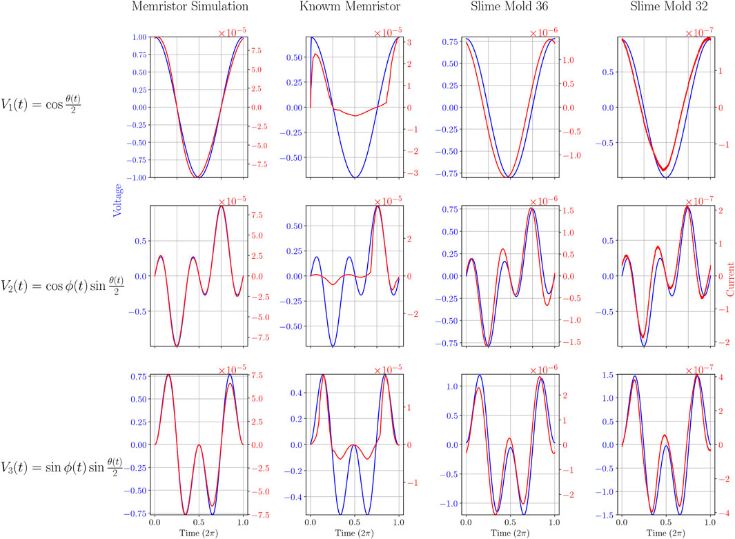
Figure 3. Voltage and Current curves over time of the four different experiments for each of the three different input signals. x- axis: time from 0 to $2\pi$, y-axis: voltage V in blue, current $\mu$A in red.

Figure 4

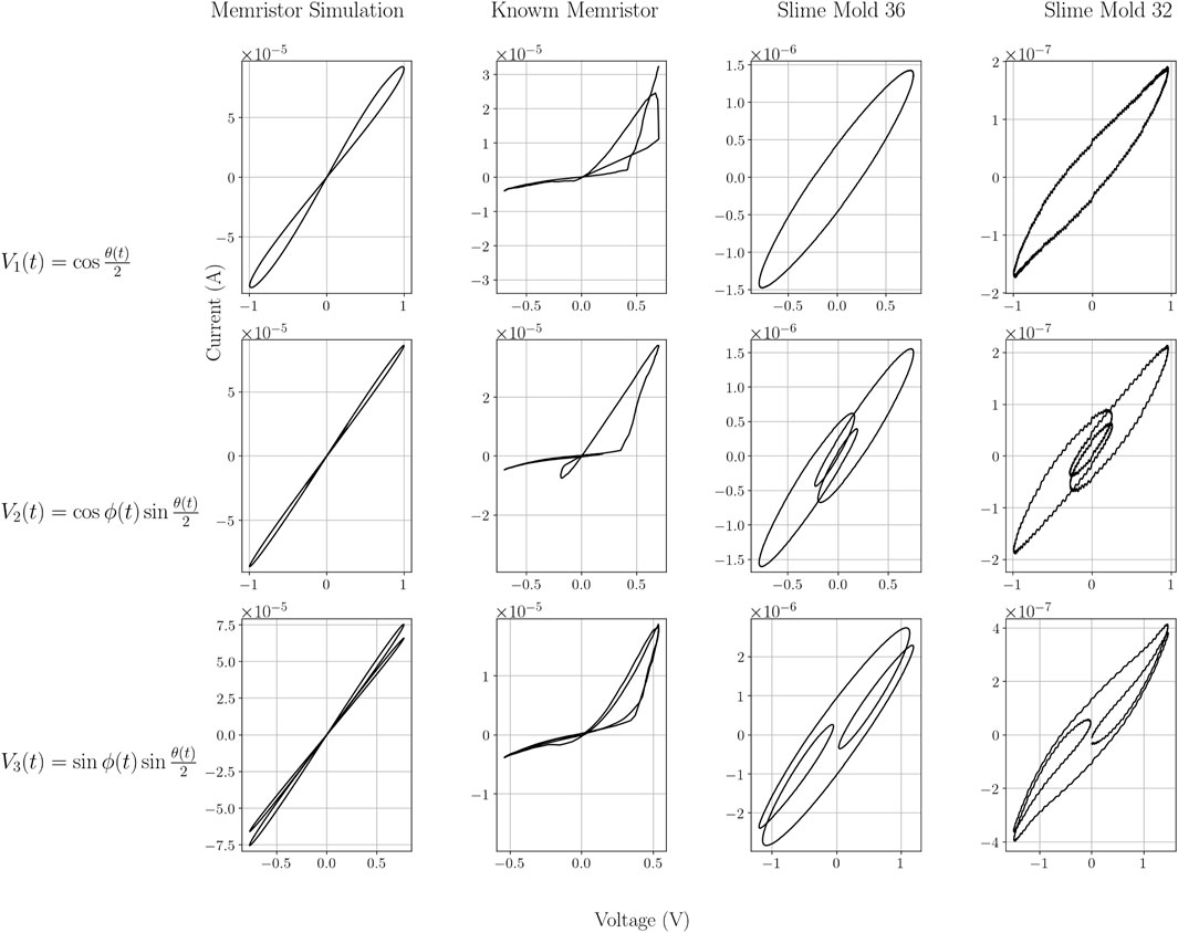
Figure 4. Current-voltage characteristic of the four different experiments for each of the three different input signals. x- axis: voltage V, y-axis: current $\mu$A.

For the slime molds, the curves differ from cycle to cycle. The biggest shift is from the first to the consecutive cycles, as the I-V curve starts at (or close to) the 0-0 point. Within the first cycle the curve then adopts a shape that is repeated for future cycles, although a slight change can be observed within each cycle, see Figure 5. In our analysis, the first cycles were never used, but the second.

Figure 5

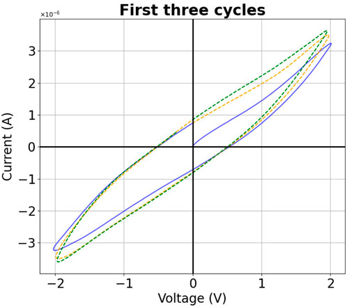
Figure 5. Color coded first three cycles of a typical slime mold measurement.

Using the data shown in Figure 4, applying Ohm’s law R = U/I results in the memristance/resistance curves shown in Figure 6. Althoughthe model (simulation) exhibits a variation of the resistance between a (positive) lower $R_{\text{min}}$ $(8.56k\mathrm{\Omega })$ and an upper $R_{\text{max}}$ $(12.645k\mathrm{\Omega })$. The physical component (Knowm memristor) switches between a low (approximately ($26k\mathrm{\Omega }$) and a high resistance (approximately ($200k\mathrm{\Omega }$) state but also shows sections where the resistance value goes from very high ($M\mathrm{\Omega }$) to very low (-$M\mathrm{\Omega }$), which typically happens as a result of the voltage being zero but the current showing non-zero values due to (parasitic) capacitance and resulting in (in this case slight) phase shift between voltage and current. Technically, in case of capacitance (or inductance), it would be necessary to calculate not memristance or resistance, but impedance Z. In the slime molds the effect of the capacitance (phase shift between voltage and current) is even more pronounced, leading to a stronger effect around areas where V is very low or 0, also leading to punctual negative impedance values. In the areas least affected by this effect the resistance is approximately $500k\mathrm{\Omega }$ for slime mold 36 and approximately $4-5M\mathrm{\Omega }$ for slime mold B. The measured current in slime mold 32 was thus an order of magnitude lower than slime mold 36, leading to the 50 Hz electric hum artefact.

Figure 6

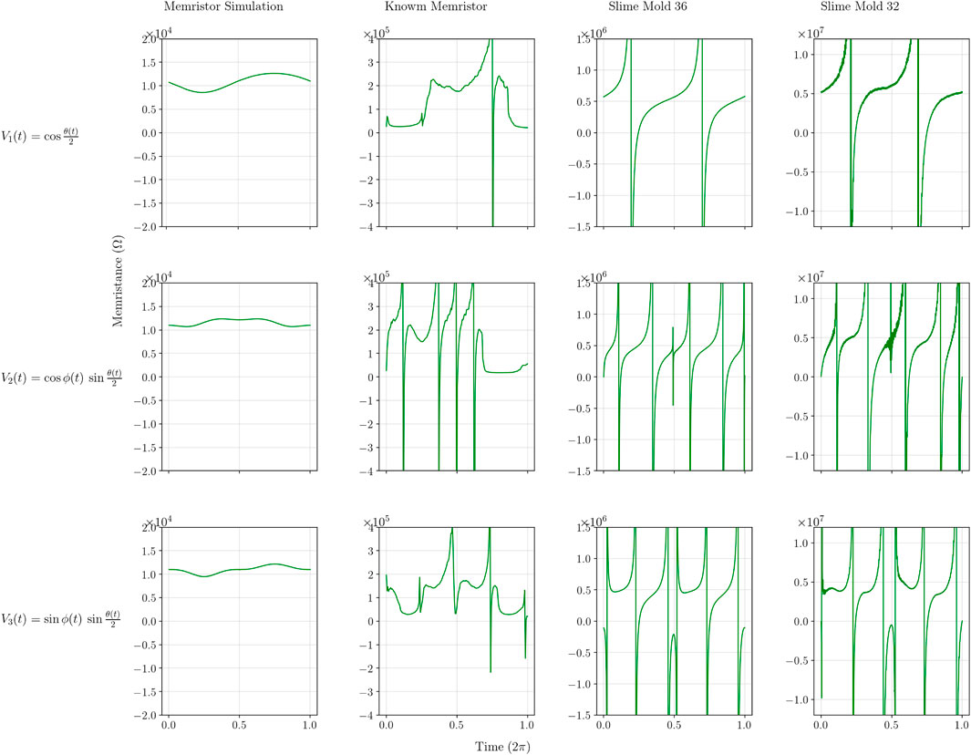
Figure 6. Memristance (Ohm) curves of the four different experiments for each of the three different input signals.

Neither the physical nor the biological components behave like ideal memristors due: a) to asymmetry between positive and negative voltages and small parasitic capacitance (physical component); and (b) no or small memristive effect and capacitance (biological component). The physical component, the Knowm memristor curve appears less smooth compared to the memristor simulation curve. The two biological component curves appear even less smooth. They exhibit sharp changes in resistance/impedance and several fluctuations even reaching negative values, indicating a behavior unlike the memristor simulation.

3.2 Slime mold electric characterization over a wider voltage and frequency range

We tested a wider range of voltages and frequencies as input signals to the slime molds to find out if a memristance would appear. We applied up to 11 different sinus inputs between 5 mV and 2 V. None of the Voltages tested resulted in pinched “8” shaped curves, all were elliptical. Results with lower voltages showed two specific outcomes. First, the slime molds themselves produce a low electric output, in these cases approximately 20 mV (or −20 mV depending on the polarization) and less than 10$\mu$A. In the cases where the input voltage is in the same order of magnitude, the a clear offset from the 0-0 point is visible. Second, the 50 Hz electrical hum was picked up more strongly at very low voltage inputs, gradually disappearing at higher voltages, see Figure 7 We also tested different frequencies ranging from 1$\mu$Hz to 100 Hz. The ultra low frequencies, below 1 mHz, were not completed in its entirety, as this would have lasted e.g. 11,5 days for a 1$\mu$Hz full cycle. The longest measurements were 1,000 s (16,67 min). Still, we identified some interesting patterns, see Figure 8 as an example. Application of very low frequencies reveal a small amount of electrical output generated by the slime molds themselves, visible as a periodic pattern on the curve. In the example with 100$\mu$Hz, 8-9 cycles can be identified in 1,000 s (111-125 s per period), at 300$\mu$Hz the effect is visible but less pronounced, almost disappear at 1 mHz. Higher frequencies, in the magnitude of 50 Hz AC, got an amplitude modulation by the 50 Hz hum, especially as multiples or fractions of 50 Hz, see Figure 9 as an example. Again, all frequency variation measurements yielded elliptical curves.

Figure 7

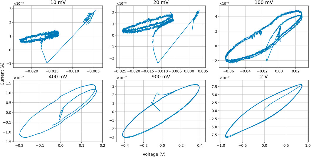
Figure 7. I-V diagrams of different sinus input voltages, including first cycle. Example shows results in slime mold nr. 43.

Figure 8

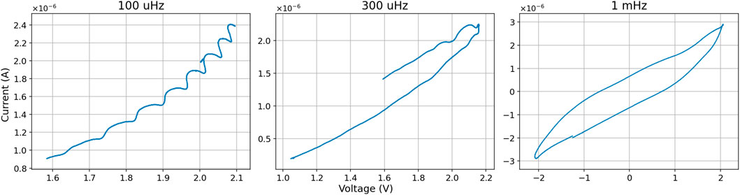
Figure 8. I-V diagrams of different very low sinus input frequencies. Example shows results in slime mold nr. 35.

Figure 9

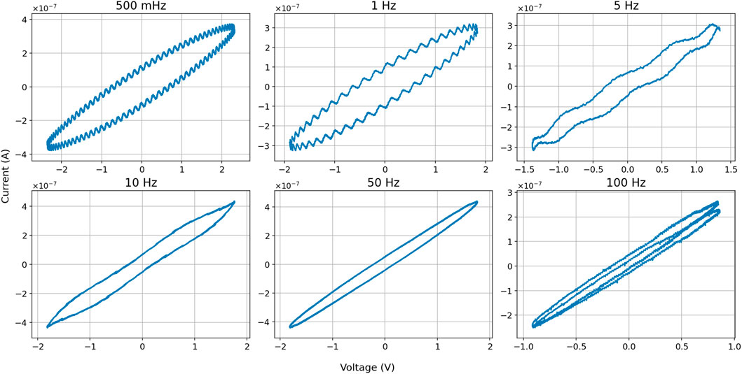
Figure 9. I-V diagrams of different “higher” sinus input frequencies. Example shows results in slime mold nr. 32.

Finally, we also measured the voltage and current of seven different slime molds with no external input. These measurements show that there is a small intrinsic electrical output of the slime molds that may change over time. In some cases (e.g. SM30 and SM32) the measured voltage was below 10 mV and did not change much over time). In another case (SM34) the output was relatively stable below −2 mV but had some periodicity (about 10 cycles in 1,000 s). Yet other measurements (e.g. SM18, SM35 and SM36) started with a higher voltage up to an absolute value of 159 mV and gradually moved towards a value closer to zero. SM35 also showed periodicity on top of the discharge, with about 8 cycles in 1,000 s, see Figure 10.

Figure 10

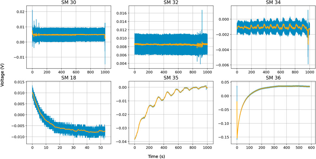
Figure 10. Slime mold electric output without external inputs. Blue line represents actual measurements, orange line is a moving average (N = 41).

3.3 I-V curve shape analysis

We analyzed all I-V measurements with a sinus input and a length below 1,000 s to find out whether they rather resemble an elliptical curve shape or a pinched figure eight. While the first points towards an RC like characteristic, the latter one is a clear and indicative sign of a memristor.

We analyzed $N=89$ living slime mold sinus I-V traces, figure-derived features were computed after robust de-spiking and zero-phase smoothing (Methods). Table 3 summarizes the per-metric classifications for the four criteria used in the majority vote (PCA_ecc, Ellipse_RMSE_cls, Pinch_Ratio_cls, Width@V0_cls) together with the final label.

Table 3

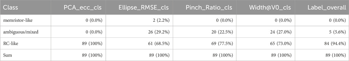
Table 3. Per-metric and overall classification counts across the analyzed dataset $(N=89)$.

At the shape level, PCA_ecc indicated RC-consistent, elongated ellipses for all traces (89/89, 100%). The ellipse-fit residual classified 61 traces as RC-like (68.5%), 26 as ambiguous (29.2%), and 2 as memristor-like (2.2%). Pinch-based evidence identified 69 RC-like (77.5%), 20 ambiguous (22.5%), and 0 memristor-like (0.0%). The zero-voltage width metric labeled 65 RC-like (73.0%), 24 ambiguous (27.0%), and 0 memristor-like (0.0%). Aggregating the four criteria by simple majority yielded an overall RC-like label for 84 traces (94.4%), with the remainder 5 (5.6%) ambiguous; no trace reached a memristor-like majority. Ambiguous outcomes typically reflected disagreement between pinch/width (weak memristive signatures) and ellipse-based criteria, or edge cases with scarce $V=0$ crossings. The two instances where the ellipse-fit residual classification mentioned memristor-like were inspected. In one case the classification of the (elliptic) shape might have been affected by a measurement artifact at the very beginning with the line going through the 0-0 point, the second one was an elliptic shape with a 50hz hum, indicating both as false positives.

Given the results of slime molds do not show memristive behavior, no further attempts were made to simulate a quantum entanglement with these components. The artifacts, including large positive and negative values up to infinity impeded further steps.

3.4 Inactive desiccated slime mold and other measurements

We carried out measurements with two sinus frequencies (7.76 mHz and 23,39 mHz) and an amplitude of 4 V (plus/minus 2 V) in two slime molds that were already 1 year 3 months and 15 days inside their test tube container. Visually the had turned brown (initially yellow/white) and appeared desiccated. The resulting I-V curves. These old slime molds produced curves that were not dissimilar to recently cultivated ones, see Figure 11.

Figure 11

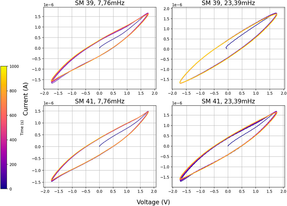
Figure 11. I-V diagrams of old slime molds >15 months, measured over 1,000 s.

Measurement with two frequencies (7.76 mHz and 23,39 mHz) for different types of water (destilled, Viennese tap water, 1% NaCl, were measured in a plastic container with electrodes 5 cm aparts, and 1% NaCl in the same test tube were we measured the slime molds), plants (cactus and basil) and food (hard cheese and yoghurt) were carried out as a comparison to the slime molds, see Figure 12. In the water samples, the degree of ions/salt in the water changes the curves significantly. Destilled water showed two pinched points in their loop, salt water was an open curve, Viennese tap water was a relatively narrow open curve, and salt water in the test tube was also more narrow than in the wider plastic container. In the plants, basil resulted in open curves, as did the cactus but which had a more pronounced non-linearity. The two tested food objects were somewhere in the middle between salt water and the cactus.

Figure 12

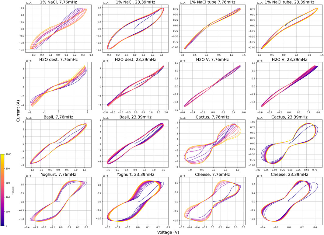
Figure 12. Set of I-V diagrams of comparative measurements, 1,000 s duration.

3.5 A replacement circuit for slime molds and alternative potential bioelectric uses of Physarum polycephalum

We modeled several potential replacement circuits of the slime mold(s) in LT Spice to generate a similar output as shown in Figure 4. The most similar results were found in the circuit with a capacitor and a resistor in series followed by a parallel capacitor and resistor. Further parametric refinement of this promising replacement circuit yielded very similar results in LT Spice as measured in the slime mold (SM36). The replacement circuit is shown in Figure 13 and the two corresponding I-V curve sets in Figure 14. The slime mold is not a totally passive device. A voltage meter can measure a voltage between 20 and 40 mV when connected directly to the slime mold. The measured voltage reduced slightly during the measurement.

Figure 13

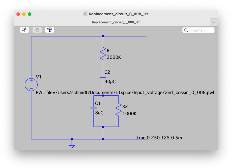
Figure 13. Final slime mold replacement circuit containing only resistors and capacitors (Schmidt et al., 2025)

Figure 14

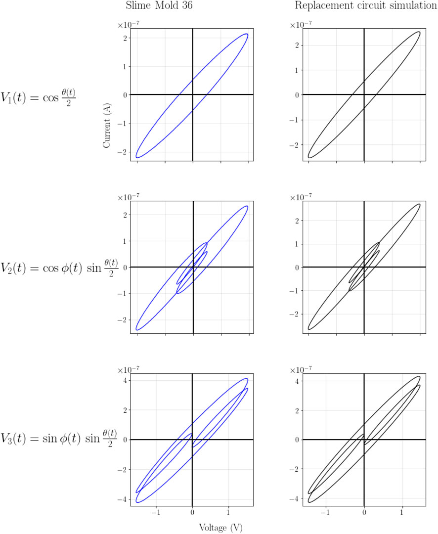
Figure 14. Comparison of the three resulting IV curves between slime mold and the replacement ciurcuit.

Using the slime mold as a “pseudo-capacitor” we applied it within some electronic circuits such as a low and high pass filter. In a low-pass filter, the cutoff frequency and level of attenuation naturally depend on the leading resistor. If we choose the resistor as $5M\mathrm{\Omega }$, the cut-off frequency is in the 100 $\mu$Hz range and the attenuation goes down to more than 8 dB at 100 mHz, after which no more attenuation is observed. Note that the attenuation between 100 $\mu$Hz and 100 mHz is steep at first but then a small hump indicates a reduction in attenuation before reaching its ultimate attenuation. The same circuit also acts as a Phase Shift Circuit with a maximum shift of −22.5° at 0.7 mHz See Figure 15. An example for a high pass filter can be seen in Figure 16 with an additional resistor of $10M\mathrm{\Omega }.$ The Bode diagram of the high-pass (like) filter shows an attenuation (red line) below a cut-off frequency of about 0.4 mHz. The same circuit also acts as a Phase Shift Circuit with a maximum shift of 90° at 1$\mu$Hz down to 0° at 1 Hz (red dotted line) Schmidt et al. (2025).

Figure 15

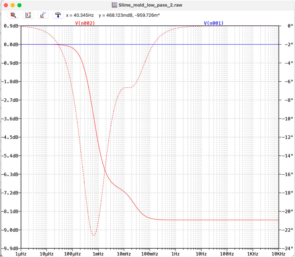
Figure 15. Bode diagram of a low pass filter with a slime mold instead of a capacitor. Red line: attenuation); red dotted line: phase shift.

Figure 16

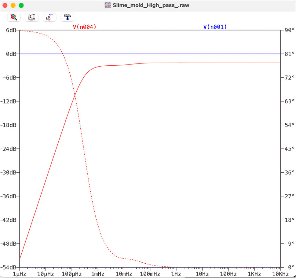
Figure 16. Bode diagram of a high pass filter with a slime mold instead of a capacitor. Red line: attenuation); red dotted line: phase shift.

The red dotted lines in Figures 15, 16 show the phase shift of these particular examples, which indicates that slime molds may also be deployed in phase shift circuits.

4 Discussion

4.1 Absence of pinched hysteresis in slime molds under tested conditions

The potential for bio-inspired materials, such as slime molds, to behave like a memristor would be of great interest due to their natural adaptability and self-organizing properties.

To find out whether or not slime molds behave like memristors, we followed the experimental works reported in (Gale et al., 2014; Braund and Miranda, 2017; Miranda and Braund, 2017; Adamatzky, 2015a). These works suggested that slime mold can behave like a memristor: a passive two-terminal electronic devices which resistance depends on the history of voltage and current that has passed through them, resulting in a distinctive pinched hysteresis loop in their I-V characteristics. However, our repeated measurements, showed that in our set-up, the slime mold does not behave like a memristor. Not a single slime mold produced a pinched hysteresis curve. While some slime mold experiments resulted in slightly S-shaped curves (see slime mold B), all of them were rather elliptical (with sinus or cosines inputs). The elliptical shape, we believe, is caused by a capacitance that is created by the cell membrane and internal cell fluids that act as electrolytes. This is comparable to the electric behavior in plants. When electrodes are inserted into a plant, they interact with the plant’s internal ionic fluids and cellular structures, creating a measurable capacitance. This phenomenon occurs because plant tissues contain conductive ionic fluids, such as sap, which facilitate the movement of electrical charges (Gao et al., 2024). Additionally, the cell membranes within the plant act as dielectric barriers, separating different conductive regions within the tissue. These biological components form an equivalent parallel resistance-capacitance circuit when connected to electrodes, allowing for the storage and separation of charges. As a result, the electrical capacitance of the system should never be zero. The capacitance measured in a plant-electrode system is influenced by various factors, including the plant’s moisture content, the type of plant tissue, and the positioning of the electrodes. For instance, a study by Dalton (1995) demonstrates that the presence of biological fluids and cell membranes ensures that the capacitance value is always non-zero, reflecting the plant’s intrinsic electrical properties.

These effects prevent the curve from passing through the origin (0,0), indicating that it might not be possible to simulate a quantum computer in a simple setup, where just electrodes are implanted without further mitigation. The slime mold is not a plant, of course, and one of its unique features is that it lacks internal cell membranes, which means that it appears like a single cell organism (with thousands of cell nuclei). This specific unique internal Bauplan, however, does not change the fact that organisms in general are (also) capacitors. See Atkinson et al. (2023) for an overview of biological capacitors in bioelectronics.

Our results showed, in all of the datasets, elliptical I-V relationships. A slight saddle, seen in some of the measurements, suggests some non-linear behavior, but not the classic hysteresis loop of a memristor. The absence of a pinched hysteresis loop suggested only weak or no memristive behavior under the tested conditions.

Why are our findings different from those reported in the literature? First, the reported memristive effect does not seem to appear in all experiments. Gale et al. Gale et al. (2016), for example wrote: “Of the eleven samples in batch 1, two exhibited good memristance curves (as in they had pinched hysteresis), the other nine exhibited open curves” and “For batch 2, which were measured at a larger voltage range (between$\pm$ 100 and $\pm$ 250 mV), eight out of eight samples showed good memristive curves”. Braund and Miranda Braund and Miranda (2017) reported a combination of pinched and open curves in their experiments, depending on the distance of the electrodes/length of slime mold tube and specific measurement parameters. In contrast to our measurement, they applied voltages that changed stepwise with steps being between ± 250 and 500 mV and time steps of 0.5, 1, 2 and 2.5 s using a Keithley 617 Programmable Electrometer, and calculated averages for the different steps. We did also test a step wise voltage increase and did not find pinched curves. Another difference was that they seemingly only used the first voltage cycle that always starts at the 0-0 origin. We, in contrast, always omitted the first cycle, as the capacitance is uncharged at the beginning. Clearly our results do not match the reports in the literature about pinched hysteresis curves. This is why we carried out such a large number (to our knowledge the largest set) of experiments to investigate memristive behavior of slime molds. It remains to be seen if future experiments will validate previous reports or confirm our findings.

4.2 Slime mold as device for other electrical circuits

The replacement circuit we created (see Figure 13) consists entirely of R and C components, and is similar, although not identical, to plant equivalent electrical circuits outlined by Van Haeverbeke et al. (2023)(see their Table 4). An additional 10-20 mV voltage source that (may) fall off continuously seems a good description of the slime molds without the nonlinear “saddles” by first approximation. Although these circuits do not represent or contain memristors, they might still be used as sub-circuits for various other types of circuits. The configuration suggests it could be useful in a number of circuits, for example a Low-Pass Filter Circuit. A low-pass filter allows low-frequency signals to pass while attenuating high-frequency signals. Usually such a subcircuit could be part of audio circuits, analog-to-digital conversion stages, or any application where it is necessary to remove high-frequency noise. Like the Low-Pass filter, the voltage divider with frequency dependence, a circuit that may serve as a frequency-dependent voltage divider, where the output voltage depends on the input frequency. This circuit can be used in circuits where frequency-based signal conditioning is required. Another option to implement the slime mold would be a Phase Shift Network that could be used to introduce a phase shift in a signal, depending on how the resistor and slime molds are connected. Phase shift networks are used in phase-shift oscillators and certain types of filters. Similarly to the low pass is the high pass filter circuit that allows high frequencies to pass while blocking low frequencies. In principle, the slime mold could also be used in several other circuits, such as RC Integrator Circuit, a RC Differentiator Circuit, a RC Time Constant, or a Snubber Circuit. Previous work has also shown that slime molds can improve microbial fuel cells when applied to the cathode side Taylor et al. (2015). This and other potential bioelectric applications seem interesting for future bioelectric deployment of the slime mold, despite it not showing memristive behavior.

Table 4

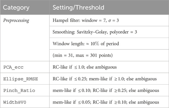
Table 4. Preprocessing settings and heuristic thresholds used for classification. Thresholds define ranges for memristor-like, RC-like, or ambiguous labels per metric.

5 Conclusion

Simulating quantum entanglement with an ideal memristor model has been demonstrated in the literature. In this work we intended to carry out this simulation using simulated memristor models, real physical/electric (Knowm Inc. memristor) and slime molds (Physarum polycephalum). Our experiments demonstrate that the biological component, Physarum polycephalum which has been described in the literature to exhibit memristive behavior turned out not to show any (significant) memristive characteristics due to its inherent capacitance. While some publications claim that slime mold could have memristive or memcapacitive characteristics, neither were detected in our experiments. Instead, we showed that slime molds could very well be described, by first approximation, with replacement circuits consisting only of resistors and capacitors. Some of the slime molds did show a slight non-linearity when going over a certain voltage threshold, but none could be characterized clearly as a memristor or a memcapacitor.

The inherent capacitance of slime mold (that is also seen in other organisms (Van Haeverbeke et al., 2023), seems to be based on the cytoplasma electrolyte, and is a characteristic that is practically impossible to change. Thus, according to our results, any electric circuit requiring a memristive behavior cannot be designed with slime molds alone. The inherent capacitance of the slime mold defies the claim that slime molds are (bio-)memristors. It remains to be seen if future experiments will identify a methodology to grow slime molds without a capacitance.

While slime molds are not memristors they can be - in a first approximation - described with an adequate replacement circuit consisting of resistors and capacitors. This RC replacement network is versatile and could be integrated as a sub-circuit in various analog circuits, including high- and low-pass filters, timing circuits, signal processing units, and phase shift networks. While slime molds could not be used to simulate quantum entanglement, they may still have a future as bioelectronic components for different types of applications.

Data availability statement

The datasets presented in this study can be found in the Mendeley repository: https://data.mendeley.com/datasets/ghm9gvwwvb/1.

Author contributions

MS: Conceptualization, Formal Analysis, Funding acquisition, Investigation, Methodology, Project administration, Resources, Software, Supervision, Validation, Visualization, Writing – original draft, Writing – review and editing. GS: Data curation, Formal Analysis, Methodology, Software, Visualization, Writing – original draft, Writing – review and editing. UR: Investigation, Methodology, Writing – review and editing. ZS: Formal Analysis, Validation, Writing – review and editing. EM: Conceptualization, Investigation, Methodology, Resources, Writing – review and editing.

Funding

The author(s) declare that financial support was received for the research and/or publication of this article. MS, GS, and UR acknowledge funding from the European Union “Mi-Hy” Project 101114746 and KIT funding for “Kunst und Wissenschaft: kreative Stoerung, Innovationsmotor oder Aesthetisierung der Forschung? - Neue Herausforderung fuer die Technikfolgeabschätzung (TA)”.

Acknowledgments

We would also like to thank Satvik Venkatesh and Andrew Adamatzky for helpful feedback on their previous slime mold electronic measurements and memfractance.

Conflict of interest

The authors declare that the research was conducted in the absence of any commercial or financial relationships that could be construed as a potential conflict of interest.

Generative AI statement

The author(s) declare that Generative AI was used in the creation of this manuscript. Generative AI was used to aid in the preparation of python scripts to analyse the data. Careful checking of the code and results were done manually to confirm its validity.

Any alternative text (alt text) provided alongside figures in this article has been generated by Frontiers with the support of artificial intelligence and reasonable efforts have been made to ensure accuracy, including review by the authors wherever possible. If you identify any issues, please contact us.

Publisher’s note

All claims expressed in this article are solely those of the authors and do not necessarily represent those of their affiliated organizations, or those of the publisher, the editors and the reviewers. Any product that may be evaluated in this article, or claim that may be made by its manufacturer, is not guaranteed or endorsed by the publisher.

References

Aaronson, S., and Gottesman, D. (2004). Improved simulation of stabilizer circuits. Phys. Rev. A 70, 052328. doi:10.1103/PhysRevA.70.052328

CrossRef Full Text | Google Scholar

Abdelouahab, M.-S., Lozi, R., and Chua, L. (2014). Memfractance: a mathematical paradigm for circuit elements with memory. Int. J. Bifurcation Chaos 24, 1430023. doi:10.1142/s0218127414300237

CrossRef Full Text | Google Scholar

Adamatzky, A. (2014). Slime mould electronic oscillators. Microelectron. Eng. 124, 58–65. doi:10.1016/j.mee.2014.04.022

CrossRef Full Text | Google Scholar

Adamatzky, A. (2015a). Slime mould processors, logic gates and sensors. Philos. Trans. A Math. Phys. Eng. Sci. 373, 20140216. doi:10.1098/rsta.2014.0216

PubMed Abstract | CrossRef Full Text | Google Scholar

Adamatzky, A. (2015b). Twenty-five uses of slime mould in electronics and computing - survey. Int. J. Unconv. Comput. 11, 449–471.

Google Scholar

Adamatzky, A., and Jones, J. (2010). Road planning with slime mould: if physarum built motorways it would route m6/m74 through newcastle. Int. J. Bifurcation Chaos 20, 3065–3084. doi:10.1142/S0218127410027568

CrossRef Full Text | Google Scholar

Adamatzky, A., and Jones, J. (2011). On electrical correlates of physarum polycephalum spatial activity: can we see physarum machine in the dark? Biophysical Rev. Lett. 06, 29–57. doi:10.1142/s1793048011001257

CrossRef Full Text | Google Scholar

Aguirre, F., Sebastian, A., Le Gallo, M., Song, W., Wang, T., Yang, J. J., et al. (2024). Hardware implementation of memristor-based artificial neural networks. Nat. Commun. 15, 1974. doi:10.1038/s41467-024-45670-9

PubMed Abstract | CrossRef Full Text | Google Scholar

Arduino (2023). Arduino uno r4 wifi documentation.

Google Scholar

Atkinson, J. T., Chavez, M. S., Niman, C. M., and El-Naggar, M. Y. (2023). Living electronics: a catalogue of engineered living electronic components. Microb. Biotechnol. 16, 507–533. doi:10.1111/1751-7915.14171

PubMed Abstract | CrossRef Full Text | Google Scholar

Bonner, J. T. (2010). Brainless behavior: a myxomycete chooses a balanced diet. Proc. Natl. Acad. Sci. U. S. A. 107, 5267–5268. doi:10.1073/pnas.1000861107

PubMed Abstract | CrossRef Full Text | Google Scholar

Borghetti, J., Snider, G. S., Kuekes, P. J., Yang, J. J., Stewart, D. R., and Williams, R. S. (2010). Memristive switches enable stateful logic operations via material implication. Nature 464, 873–876. doi:10.1038/nature08940

PubMed Abstract | CrossRef Full Text | Google Scholar

Boussard, A., Fessel, A., Oettmeier, C., Briard, L., Dobereiner, H. G., and Dussutour, A. (2021). Adaptive behaviour and learning in slime moulds: the role of oscillations. Philos. Trans. R. Soc. Lond B Biol. Sci. 376, 20190757. doi:10.1098/rstb.2019.0757

PubMed Abstract | CrossRef Full Text | Google Scholar

Braund, E., and Miranda, E. (2017). On building practical biocomputers for real-world applications: receptacles for culturing slime mould memristors and component standardisation. J. Bionic Eng. 14, 151–162. doi:10.1016/s1672-6529(16)60386-4

CrossRef Full Text | Google Scholar

Chattopadhyay, A., and Rakosi, Z. (2011). “Combinational logic synthesis for material implication,” in 2011 IEEE/IFIP 19th international conference on VLSI and system-on-chip (Hong Kong, China: ieee). doi:10.1109/VLSISoC.2011.6081665

CrossRef Full Text | Google Scholar

Chua, L. (1971). Memristor: the missing circuit element. IEEE Trans. Circuit Theory 18, 507–519. doi:10.1109/tct.1971.1083337

CrossRef Full Text | Google Scholar

Chua, L. (2018). How we predicted the memristor. Nat. Electron. 1, 322. doi:10.1038/s41928-018-0074-4

CrossRef Full Text | Google Scholar

Dalton, E. N. (1995). In-situ root extent measurements by electrical capacitance methods. Plant Soil 173, 157–165. doi:10.1007/bf00155527

CrossRef Full Text | Google Scholar

Di Ventra, M., Pershin, Y., and Chua, L. (2009). Circuit elements with memory: memristors, memcapacitors, and meminductors. Proc. IEEE 97, 1717–1724. doi:10.1109/jproc.2009.2021077

CrossRef Full Text | Google Scholar

Fyrigos, I.-A., Ntinas, V., Karafyllidis, I., Sirakoulis, G., Karakolis, P., and Dimitrakisc, P. (2018). Early approach of qubit state representation with memristors.

Google Scholar

Gale, E., Adamatzky, A., and de Lacy Costello, B. (2014). Slime mould memristors. BioNanoScience 5, 1–8. doi:10.1007/s12668-014-0156-3

CrossRef Full Text | Google Scholar

Gale, E., Aadamatzky, A., and de Lacy Costello, B. (2016). On the memristive properties of slime mould. Springer 21 (5), 75–90. doi:10.1007/978-3-319-26662-6_4

CrossRef Full Text | Google Scholar

Gao, C., Gu, Y., Liu, Q., Lin, W., Zhang, B., Lin, X., et al. (2024). All plant-based compact supercapacitor in living plants. Small 20, e2307400. doi:10.1002/smll.202307400

PubMed Abstract | CrossRef Full Text | Google Scholar

Huang, Y., Ando, T., Sebastian, A., Chang, M.-F., Yang, J., and Xia, Q. (2024). Memristor-based hardware accelerators for artificial intelligence. Nat. Rev. Electr. Eng. 1, 286–299. doi:10.1038/s44287-024-00037-6

CrossRef Full Text | Google Scholar

Ielmini, D., and Milo, V. (2017). Physics-based modeling approaches of resistive switching devices for memory and in-memory computing applications. J. Comput. Electron 16, 1121–1143. doi:10.1007/s10825-017-1101-9

PubMed Abstract | CrossRef Full Text | Google Scholar

Jebali, F., Majumdar, A., Turck, C., Harabi, K. E., Faye, M. C., Muhr, E., et al. (2024). Powering ai at the edge: a robust, memristor-based binarized neural network with near-memory computing and miniaturized solar cell. Nat. Commun. 15, 741. doi:10.1038/s41467-024-44766-6

PubMed Abstract | CrossRef Full Text | Google Scholar

Karafyllidis, I., Sirakoulis, G., and Dimitrakis, P. (2018). “Representation of qubit states using 3d memristance spaces: a first step towards a memristive quantum simulator,” in Proceedings of the 14th IEEE/ACM international symposium on nanoscale architectures (Athens, Greece: NANOARCH ’18), 163–168. doi:10.1145/3232195.3232197

CrossRef Full Text | Google Scholar

Karafyllidis, I., Sirakoulis, G., and Dimitrakis, P. (2019). Memristive quantum computing simulator. IEEE Trans. Nanotechnol. 18, 1015–1022. doi:10.1109/tnano.2019.2941763

CrossRef Full Text | Google Scholar

Kishimoto, U. (1958). Rhythmicity in the protoplasmic streaming of a slime mold, physarum polycephalum. i. a statistical analysis of the electric potential rhythm. J. Gen. Physiol. 41, 1205–1222. doi:10.1085/jgp.41.6.1205

PubMed Abstract | CrossRef Full Text | Google Scholar

Lehtonen, E., Poikonen, J. H., and Laiho, M. (2010). Two memristors suffice to compute all boolean functions. Electron. Lett. 46, 230–231. doi:10.1049/el.2010.3407

CrossRef Full Text | Google Scholar

Luo, L., Dong, Z., Duan, S., and Lai, C. (2020). Memristor-based stateful logic gates for multi-functional logic circuit. IET Circuits, Devices Syst. 14, 811–818. doi:10.1049/iet-cds.2019.0422

CrossRef Full Text | Google Scholar

Miranda, E., and Braund, E. (2017). A method for growing bio-memristors from slime mold. J. Vis. Exp., e56076. doi:10.3791/56076

PubMed Abstract | CrossRef Full Text | Google Scholar

Nakagaki, T., Yamada, H., and Toth, A. (2000). Maze-solving by an amoeboid organism. Nature 407, 470. doi:10.1038/35035159

PubMed Abstract | CrossRef Full Text | Google Scholar

Park, S. O., Jeong, H., Park, J., Bae, J., and Choi, S. (2022). Experimental demonstration of highly reliable dynamic memristor for artificial neuron and neuromorphic computing. Nat. Commun. 13, 2888. doi:10.1038/s41467-022-30539-6

PubMed Abstract | CrossRef Full Text | Google Scholar

Pershin, Y., La Fontaine, S., and Di Ventra, M. (2009). Memristive model of amoeba learning. Phys. Rev. E 80, 021926. doi:10.1103/physreve.80.021926

PubMed Abstract | CrossRef Full Text | Google Scholar

Saigusa, T., Tero, A., Nakagaki, T., and Kuramoto, Y. (2008). Amoebae anticipate periodic events. Phys. Rev. Lett. 100, 018101. doi:10.1103/PhysRevLett.100.018101

PubMed Abstract | CrossRef Full Text | Google Scholar

Schmidt, M., Seyfried, G., Reutina, U., Seskir, Z., and Miranda, E. R. (2025). Electrical characterization of the alleged bio-memristor physarum polycephalum. MRS Adv. doi:10.1557/s43580-025-01198-8

CrossRef Full Text | Google Scholar

Sheridan, P. M., Cai, F., Du, C., Ma, W., Zhang, Z., and Lu, W. D. (2017). Sparse coding with memristor networks. Nat. Nanotechnol. 12, 784–789. doi:10.1038/nnano.2017.83

PubMed Abstract | CrossRef Full Text | Google Scholar

Snider, G. (2003). “Molecular-junction-nanowire-crossbar-based neural network,”. United States: HP Inc Hewlett Packard Enterprise Development LP.

Google Scholar

Snider, G., Amerson, R., Carter, D., Abdalla, H., Qureshi, M., Leveille, J., et al. (2011). From synapses to circuitry: using memristive memory to explore the electronic brain. Computer 44, 21–28. doi:10.1109/mc.2011.48

CrossRef Full Text | Google Scholar

SparkFun (2010). Dht22 temperature-humidity sensor datasheet

Google Scholar

Strukov, D. B., Snider, G. S., Stewart, D. R., and Williams, R. S. (2008). The missing memristor found. Nature 453, 80–83. doi:10.1038/nature06932

PubMed Abstract | CrossRef Full Text | Google Scholar

Taylor, B., Adamatzky, A., Greenman, J., and Ieropoulos, I. (2015). Physarum polycephalum: towards a biological controller. Biosystems 127, 42–46. doi:10.1016/j.biosystems.2014.10.005

PubMed Abstract | CrossRef Full Text | Google Scholar

Tim, T. V. f. (2021). Physarum polycephalum sur souche. Image available on Wikimedia Commons. Licensed under CC BY-SA 4.0.

Google Scholar

Van Haeverbeke, M., De Baets, B., and Stock, M. (2023). Plant impedance spectroscopy: a review of modeling approaches and applications. Front. Plant Sci. 14, 1187573. doi:10.3389/fpls.2023.1187573

PubMed Abstract | CrossRef Full Text | Google Scholar

Wohlfarth-Bottermann, K. E. (1979). Oscillatory contraction activity in physarum. J. Exp. Biol. 81, 15–32. doi:10.1242/jeb.81.1.15

PubMed Abstract | CrossRef Full Text | Google Scholar

Yao, P., Wu, H., Gao, B., Tang, J., Zhang, Q., Zhang, W., et al. (2020). Fully hardware-implemented memristor convolutional neural network. Nature 577, 641–646. doi:10.1038/s41586-020-1942-4

PubMed Abstract | CrossRef Full Text | Google Scholar