Direct Connection Between Auroral Oval Streamers/Flow Channels and Equatorward Traveling Ionospheric Disturbances

1 Introduction

Heating and momentum transfer to the upper atmosphere within the auroral oval can lead to neutral atmospheric gravity waves. While shorter-period (≲30 min) waves are dampened and thus cannot propagate far from their source (Richmond, 1978), longer-period waves (≳60 min) can move large distances from the auroral region toward the equator. As a result of ion–neutral collisions, these neutral atmospheric waves can be seen in the ionosphere as waves in electron density (Hines, 1960; Francis, 1975; Richmond, 1978; Hunsucker, 1982), referred to as large-scale traveling ionospheric disturbances (LSTIDs). These large-scale waves may be important for transporting auroral region energy to mid- and low-latitudes (Richmond, 1979). The total electron content (TEC) from the Global Navigation Satellite System (GNSS) receiver network gives the two-dimensional and temporal structure of LSTIDs (Zakharenkova et al., 2017, and references therein; Zhang et al., 2019a), and has shown their spatial sizes to be larger than 1,000 km and horizontal speeds of 400–1,000°m/s. LSTID’s spatial and temporal structure has also been investigated using 630 nm airglow emissions (Kubota et al., 2001; Ogawa et al., 2002; Shiokawa et al., 2007), SuperDARN HF radars (e.g., Bristow et al., 1994; Hayashi et al., 2010; Frissell et al., 2014), and multipoint ionosondes (e.g., Shiokawa et al., 2002).

It is well known that auroral zone disturbances (e.g., Hajkowicz, 1991) with magnetic bays (e.g., Ding et al., 2008) can lead to LSTIDs propagating equatorward from the nightside auroral oval. Occurrence rates increase with increasing geomagnetic activity (Tsugawa et al., 2004), and duration of activity has been associated with the duration of LSTID activity (Davis, 1971). Magnetic bays result from different classes of auroral disturbances, including substorms and poleward boundary intensifications (known as “PBIs”), which are intensifications along the auroral poleward boundary. Auroral forms that extend equatorward from PBIs to lower latitudes are known as “auroral streamers” and can give large magnetic bays (Lyons, 2000; Lyons et al., 2013) as can omega bands (Jorgensen et al., 1999), which appear in the midnight to dawn sector. Substorms include auroral streamers, with the streamers being the dominant contributor to the magnetic bays of the substorm expansion phase (Nishimura et al., 2012; Lyons et al., 2013), but streamers are also common without the occurrence of a substorm.

Previous studies had used ground magnetic observations without auroral observations to detect auroral disturbances, and thus were not able to identify the specific type of disturbance that leads to a nightside LSTID. To overcome this limitation, in our previous study (Lyons et al., 2019), we used auroral images from the white-light all sky imager (ASI) array of the Time History of Events and Macroscale Interactions during Substorms (THEMIS), giving high temporal and spatial resolution continent-scale coverage over the North American auroral zone (Mende et al., 2008) and allowing the identification of the different types of auroral oval disturbances. We related these disturbances to LSTIDs as seen in vertical total electron content (TEC) measurements over North America (Coster et al., 2003; Rideout and Coster, 2006; Vierinen et al., 2016) and in 630 nm emissions from the Midlatitude Allsky-imaging Network for Geospace Observations (MANGO) ASI array over the western United States. Time periods with LSTIDs were found to start and stop with the initiation and cessation of overall periods of geomagnetic activity, consistent with the well-established association of LSTIDs with activity. Furthermore, many of LSTIDs were found to be associated with appropriate time delay to a specific auroral disturbance, suggesting that individual LSTIDs can be driven by identifiable auroral disturbances. We found LSTIDs to be associated with substorms and with auroral streamers in the absence of a substorm. Due to ground magnetic field depressions during substorms being directly related to streamers (Lyons et al., 2013), we suggested that auroral streamer disturbances may be the primary driver of individual LSTIDs seen on the nightside, independent of whether the streamers occur during a substorm. Auroral streamers result from the electron precipitation lying approximately adjacent to mesoscale flow channels (Gallardo-Lacourt et al., 2014), which are related to electric fields that map along field lines from the ionosphere to the magnetosphere (where they are often referred to as flow bursts) and move with an equatorward (earthward) component within the ionosphere (magnetosphere). Thus, the above suggestion would imply that the flows, electric fields, and electron precipitation associated with mesoscale flow channels drive the heating and momentum transfer that gives rise to the neutral atmospheric gravity waves that appear as LSTIDs. In the study by Lyons et al. (2019), we also found indications that a disturbance should have sufficiently large ground magnetic perturbation (ΔB) in order to lead to a detectable LSTID.

In the present study, we take advantage of simultaneous oval imaging, radar flows, and TEC over Alaska to examine whether, as suggested in our previous study, there is a direct connection of LSTIDs to auroral streamers and associated flow channels having a significant ΔB. The auroral observations allow us to identify auroral streamers, and the TEC observations allow us to detect TEC variations by both the electron precipitation associated with the streamers and by TIDs propagating equatorward from the equatorward boundary of the auroral oval. Radar observations, when available, allow us to directly detect the flow channels. Furthermore, the observations over Alaska allow us to take advantage of TEC coverage in both auroral and subauroral latitudes to see how TEC first increases within the auroral oval and then connects to TIDs propagating to lower latitudes. This overcomes the limitation in our previous study from the latitudinal gap between the ASIs within the auroral zone and the mid-latitude TEC measurements over the continental United States. Since the TIDs we observe are propagating equatorward from the auroral oval as in our previous study, they are likely LSTIDs. However, we do not have the continent-wide TEC coverage necessary to demonstrate that they are large scale.

2 Methodology

We started with 14 nights that were selected for having good auroral viewing from Poker Flat, Alaska. Of these, 11 were used in our previous substorm-related studies (Lyons, et al., 2021a; Lyons et al., 2021b), and the three others had been selected for other studies. We narrowed this list to seven nights that had clear observable flow channels and/or auroral streamers and did not have ambiguities due to multiple flow channels and streamers.

We use the Poker Flat Incoherent Scatter Radar (PFISR) data product that gives flow vectors along the radar magnetic meridian from a best fit to line-of-sight (LOS) flow velocities along all PFISR beams using the assumption that longitudinal variations within the radar field-of-view (FOV) can be neglected (Nicolls and Heinselman, 2007). We use only flow vectors having an estimated error magnitude less than both the flow magnitude and 1 km/s. Super Dual Auroral Radar Network (SuperDARN) observations are also included when and where echoes are available. We show these observations as maps of flow vectors obtained with the Bristow et al. (2016) technique, which gives spatial resolution that is set by the underlying measurements rather than by the smoothing inherent in the global fits using a coarse grid that are typically used for global SuperDARN convection maps. The vectors are determined by the local LOS observations and the divergence-free condition. They are not strongly influenced by information beyond a few grid cell’s distance so that localized steep gradients can be obtained without significantly influencing the remainder of the vector domain.

Figure 1 displays the coverage of the PFISR radar beams over Alaska (orange contour), and the Poker Flat green line (green circle) and THEMIS white light (dashed circles) ASIs having coverage that includes Alaska. Locations of ground magnetometer stations from which we show data are indicated.

FIGURE 1

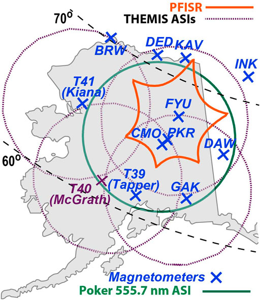
FIGURE 1. FOVs of the Poker Flat 557.7 nm images, the THEMIS ASIs in the Alaskan sector, and the PFISR radar. Also shown are ground magnetometer locations. These include the THEMIS ASI stations, except that we do not use magnetometer data from T40. IAGA station names are used (see https://supermag.jhuapl.edu/ for station details).

To detect traveling ionospheric disturbances, we analyze global navigation satellite system (GNSS) TEC observations of differential TEC values of ΔTEC, as described in the study by Zhang et al. (2017) and Coster et al. (2017) and used in our previous study. They were derived at 1 min cadence by subtracting a smooth background TEC variation determined by a low-pass Savitzky–Golay filter (Savitzky and Golay, 1964). The filter uses least squares fitting of successive subsets of windows of a given length (e.g., 30 or 60 min) involving time-adjacent TEC data points from the same GNSS satellite–receiver pair and a linear basis function set. Thus, this filter removes high-frequency fluctuation from data while maximizing the preservation of the original shape and features of the signal. A 15° cutoff elevation for ground–satellite ray paths was used to eliminate data close to the horizon where the measurement uncertainty can be large. Data at the start and the end of each continuous segment from the same GNSS satellite–receiver pair were disregarded to avoid potential “edge” effects (Zhang et al., 2019b). Similar differential TEC analysis methods have been employed extensively (e.g., Saito et al., 1998; Tsugawa et al., 2007; Ding et al., 2008; Azeem et al., 2015). The accuracy of this method is based on the accuracy of the GNSS phase measurement, which is less than 0.03 TEC units (Coster et al., 2012), as all satellite and receiver bias terms cancel out.

Note that using a 30-min window could inhibit the detection of anything other than the first wave of a chain of waves with period larger than 30 min. However, Ding et al. (2008) found that most (79%) LSTID waves are solitary waves (i.e., a single perturbation pulse), and only 21% appear to be part of a wave chain. We are examining waves directly driven by a flow channel, and these waves would likely be initiated impulsively. If a flow channel were to lead to a chain of waves, we might only detect the first and largest one. But it is the impulsive response that we are looking for as a test of the proposed direct driving.

3 Analysis

We start with two events for which the TEC coverage shows the best two-dimensional evidence for a direct connection between streamers and ensuing TIDs. The next three events show the direct connection for events having radar coverage, showing the flow channels associated with streamers and their connection to TIDs. The final two events have clear flow channels but substantially weaker ground magnetic depressions. These indicate that a flow channel must be associated with a sufficiently large ionospheric current to lead to a detectable LSTID.

3.1 March 2 and 1, 2017: Two-Dimensional TEC Coverage Showing Clear TIDs

Figure 2 shows an overview of observations from a period that included a substorm with onset at 0955:30 UT on March 2, 2017. The keograms on the left are, from top to bottom, 557.7 nm emissions from the Poker Flat ASI, vertical TEC, and vertical ΔTEC with two different scales. The keograms are along the PFISR magnetic meridian and cover available data over the entire range of Alaska magnetic longitudes (240–285°).

FIGURE 2

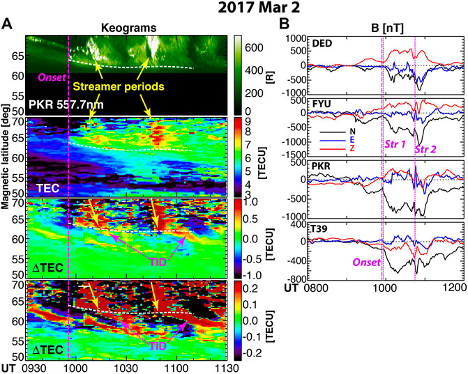
FIGURE 2. Overview of observations from a period that included a substorm with onset at 0,955:30 UT on March 2, 2017. Keograms on the (A) are, from top to bottom, 557.7 nm emissions from the Poker Flat ASI, vertical TEC, and vertical ΔTEC with two different scales along the PFISR magnetic meridian. Ground magnetometer observations are shown on the panel (B) from stations approximately along the Poker Flat meridian stacked from lower to higher latitudes.

The substorm onset appears as a small brightening within the equatorward portion of the auroral oval at magnetic latitude Λ ∼ 64°. As seen in the full ASI images in the movie Additional File S1, multiple streamers started soon before 10 UT, and then a large streamer near the Poker Flat meridian extended equatorward from the poleward expanded auroral poleward boundary starting at ∼1006 UT and reached the auroral equatorward boundary at ∼1010 UT. This streamer can be seen in the auroral keogram of Figure 2 and also, as a result of ionization from the electron precipitation, in the TEC keogram and quite clearly in the upper ΔTEC keogram (−1 to +1 TECU scale). The auroral activity decreased at ∼1020 UT, and then another group of streamers initiated at ∼1040 UT. As seen by the magnetograms in Figure 2B, the northward ground N-component (local magnetic north) started an abrupt substantial several hundred nT drop with the initiation of the two periods of streamers.

Notice that the equatorward moving TEC enhancements associated with the streamers do not stop at the oval equatorward boundary but appear to continue equatorward at reduced levels below that boundary. (The white dashed curves in the left side of Figure 2 show the estimated equatorward boundary of the auroral oval based on the ASI and TEC measurements.) The continuation is seen clearly in the lower ΔTEC panel (−0.2 to + 0.2 TECU scale) of Figure 2, where the dark red color of the streamers along the PFISR meridian can be seen to directly connect to equatorward moving dark red features having a lower slope (slower equatorward speed) than those of the streamers. The equatorward moving region equatorward of the oval is not the streamer-related flow channel and is supported by its different equatorward speed, implying a transition to the equatorward phase speed of a TID related to the streamer. This indicates a direct connection between the auroral streamers and a TID.

Figure 3 shows a sequence of the auroral images during the period of interest (557.7 nm emissions from the Poker Flat ASI with THEMIS ASI white light emissions in regions outside the Poker Flat ASI field-of-view, FOV) overlaid with all available ΔTEC measurements over the Alaska sector. Additional File S1 shows these panels every 30°s as a movie. Just at the time of substorm onset (Figure 3A), at Λ ≈ 66°, ΔTEC shows no enhancement within the auroral oval. ΔTEC can be seen to have enhanced within the oval after onset (Figure 3B) as the oval expanded poleward and equatorward extending streamers formed. Clearly discernible streamers are identified by yellow arrows in Figures 3B–D. A longitudinally extended region of ΔTEC enhancement then starts to move equatorward from the oval at ∼1002 UT, as encircled qualitatively with a yellow curve in Figure 3C (1007 UT). As encircled by the yellow curves in Figures 3D–H, this region continues to move equatorward as a detectable TID (most likely a LSTID) until ∼1054 UT. Following the initiation of the second group of streamers at ∼1040 UT (clearly discernible streamers are identified in Figures 3G,H), a second TID can clearly be seen moving equatorward from near the equatorward boundary of the auroral oval starting at ∼1050 UT. This TID is identified by the second set of encircling yellow curves in Figures 3H,I and continued to be discernible until ∼1129 UT. Both TIDs can be seen to have propagated from the equatorward boundary of the auroral oval at Λ ≈ 62°– Λ ≈ 55°, with data coverage being more limited at lower Λ.

FIGURE 3

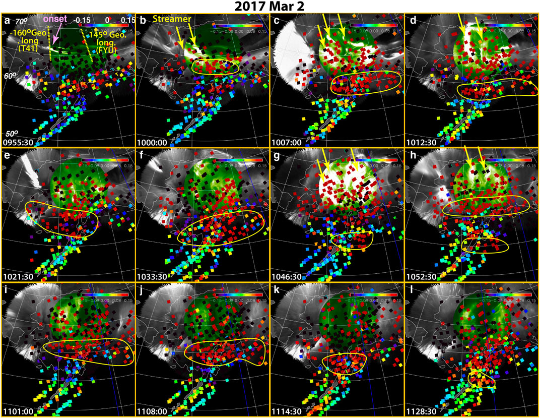
FIGURE 3. Sequence of the auroral images during the period of interest on March 2, 2017 (557.7 nm emissions from the Poker Flat ASI with THEMIS ASI white light emissions in regions outside the Poker Flat ASI field-of-view, FOV), overlaid with all available ΔTEC measurements over the Alaska sector. Yellow curves encircle equatorward moving regions of ΔTEC enhancements equatorward of the auroral oval. Dark blue line is the magnetic midnight meridian and longitude lines are spaced 15° apart.

A different way to visualize the connection between the streamers and the TID is given in Figure 4, which shows all TEC and ΔTEC data points within 5° geographic longitude bins from west of, to near, Poker Flat (−147.4° longitude). This covers the longitude range of the first set of streamers, as seen in Figure 3 and Supplementary Material S1 (note the longitude lines in these plots are spaced by 15°). The second set of streamers also extends over this longitude range and additionally somewhat further to the east. In the TEC panels, we can see these two equatorward moving regions of enhanced ionization, the first from ∼1000 to 1020 UT and the second from ∼1035 to 1100 UT. These periods correspond to the two streamer periods, indicating that they result from the electron precipitation producing the streamer auroral emissions.

FIGURE 4

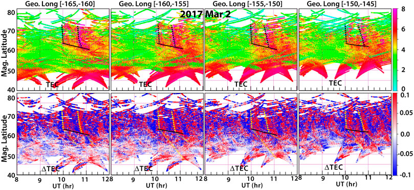
FIGURE 4. All TEC and ΔTEC data points within 5° geographic longitude bins from west of, to near, Poker Flat (−147.4° longitude) on March 2, 2017. The black solid curves give an approximation of the equatorward boundary of the electron auroral oval based on the auroral emissions in Figures 2, 3. The initial time edges of streamer ΔTEC enhancement regions are marked with yellow longer dashed lines (black dashed in the TEC panels). Initial edges of the more equatorward regions of equatorward moving ΔTEC enhancement are marked by yellow shorter dashed lines.

The black solid curves in Figure 4 give an approximation of the equatorward boundary of the electron auroral oval based on the auroral emissions in Figures 2, 3 and the TEC measurements. Note that the two regions of enhanced TEC appear to extend equatorward of the black curves but move equatorward at a different (slower) speed than does the enhancement due to the streamers. These are the TIDs identified in Figures 2, 3. The connection between the two streamer TEC enhancements and the more equatorward TEC enhancements of the TIDs can be seen clearly in the ΔTEC panels in the lower half of Figure 4. Here, initial time edges of the streamer regions as visually estimated from the plots are marked with a yellow longer dashed line (black dashed in the TEC panels), and the initial edges of the more equatorward regions are marked by a yellow shorter dashed line. The change of slope can be seen to have occurred quite near the black curves, indicating the direct connection between the sets of streamers and the two TIDs. In this case, it appears to not be single streamers that drive the TIDs but groups of streamers extending over a sector ∼15–20° wide in longitude and associated with fairly strong ground N magnetic decreases and thus fairly strong westward currents in the ionosphere. This can be seen from the auroral images in Figure 3 and Supplementary Material S1, and from the TEC enhancements of the streamers occurring over the 15–20° of longitude included in Figure 4.

Figure 5 shows a sequence of the auroral images overlaid with all available ΔTEC measurements over the Alaska sector during the period of interest of a substorm with onset at 0954:00 UT on March 1, 2017. Additional File S2 shows these panels every 30°s as a movie. As with the previous event, there were two separate periods of streamers, with the first extending from ∼0955 UT (soon after onset) to ∼1020 UT, and, while viewing conditions were partially obscured by clouds, the second started at ∼1035 UT. Hundreds of nT ground N-component decreases were observed for both.

FIGURE 5

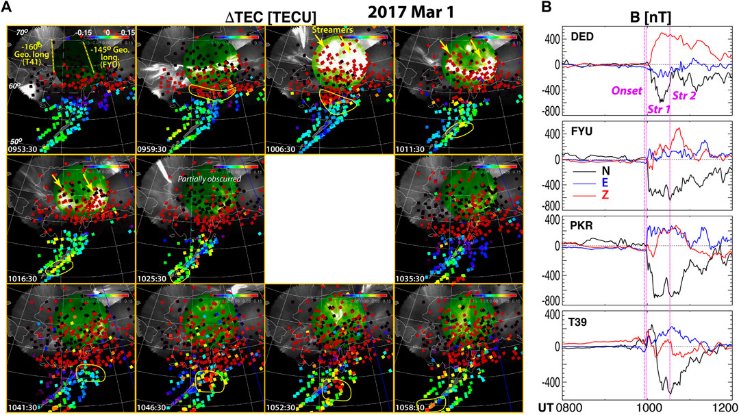
FIGURE 5. (A) Sequence of the auroral images during the period of interest on March 1, 2017 (557.7 nm emissions from the Poker Flat ASI with THEMIS ASI white light emissions in regions outside the Poker Flat ASI field-of-view, FOV), overlaid with all available ΔTEC measurements over the Alaska sector. Yellow curves encircle equatorward moving regions of ΔTEC enhancements equatorward of the auroral oval. The blank square separates the time periods of the two TIDs. Dark blue line is the magnetic midnight meridian, and longitude lines are spaced 15° apart. (B) Ground magnetometer observations from stations approximately along the Poker Flat meridian stacked from lower to higher latitudes.

Figure 6 shows the TEC and ΔTEC data within 5° geographic longitude bins from west of, to near, Poker Flat. The two sets of streamers extended over and somewhat further to the east of this longitude range. In the TEC and ΔTEC panels, we can see these two equatorward moving regions of enhanced ionization. A connection to the two equatorward propagating TIDs can be seen in the ΔTEC panels, and the slower equatorward speed of the TIDs than that of the TEC enhancement of the streamers is clearly seen. The front edge of the TID shows in the ΔTEC plots as a transition from dark blue to dark red as in Figure 4 for the second TID and for the first TID below Λ ≈ 56°. For the first TID, the transition at the auroral equatorward boundary is more subtly from blue to mostly white (ΔTEC = 0), with the transition still being near to somewhat above the 0.03 resolution of the ΔTEC measurements. This is because of the region of strong auroral TEC seen in the TEC panels that brings the auroral equatorward boundary equatorward from ∼10 to ∼1030 UT. This enhances the sliding 30 min average that is subtracted to obtain the ΔTEC values, thus reducing the magnitude that is calculated for the ΔTEC of the TID. As with the previous case, it appears that each TID is driven by a group of streamers extending over a longitude sector ∼15–20° in longitude and associated with fairly strong ground N magnetic decreases.

FIGURE 6

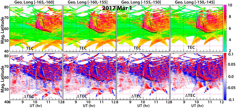
FIGURE 6. Average TEC and ΔTEC over 5° geographic longitude increments from west of, to near, Poker Flat on March 1, 2017, in the same format as Figure 4.

3.2 November 21, 2012, and March 15 and 9, 2013: Radar Coverage of Flow Channels

Figure 7 shows observations on November 21, 2012, when there was a substorm onset at 0803:20 UT during a period when PFISR was operating, and there were sufficient SuperDARN echoes available in regions of interest to provide some two-dimensional flow coverage. The top left portion of the figure shows Poker Flat ASI 557.7 nm emissions with THEMIS ASI white light emissions in regions outside the Poker Flat ASI FOV overlaid with PFISR flow vectors along the radar magnetic meridian. The lower portion shows broader THEMIS ASI mosaics over a larger area overlaid with SuperDARN flow vectors. Flow vectors are scaled by color and length, with the foot of the arrow being at the location of the measurement. Heavier flow vector arrows are at points with a LOS flow measurement. The further from a region of heavier arrows, the more the flows revert to a statistical model.

FIGURE 7

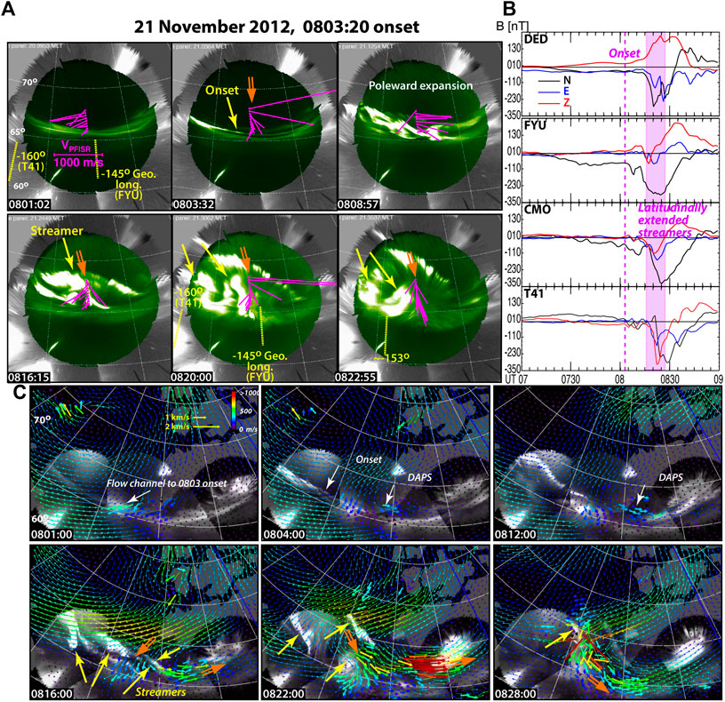
FIGURE 7. Observations on November 21, 2012, during a period when PFISR was operating, and there were sufficient SuperDARN echoes available in regions of interest to provide some two-dimensional flow coverage. (A) Poker Flat ASI 557.7 nm emissions with THEMIS ASI white light emissions in regions outside the Poker Flat ASI FOV overlaid with PFISR flow vectors along the radar magnetic meridian. (B) Ground magnetometer observations from stations approximately along the Poker Flat meridian stacked from lower to higher latitudes. (C) THEMIS ASI mosaics over a larger area overlaid with SuperDARN flow vectors. Flow vectors are scaled by color and length, with the foot of the arrow being at the location of the measurement. Dark blue line is the magnetic midnight meridian, and longitude lines are spaced 15° apart. Heavier flow vector arrows are at points with a LOS flow measurement. The further from a region of heavier arrows, the more the flows revert to a statistical model. Yellow arrows point toward streamers and orange arrows indicate observed streamer-related flows.

Both the PFISR and SuperDARN flow measurements show an enhancement of an equatorward component of the flows pointing to near the location of substorm onset as seen in the aurora, which is a common feature signifying an earthward flow channel within the plasma sheet that likely leads to the onset (Nishimura et al., 2010; Lyons et al., 2021a). An enhancement of eastward flow is seen just poleward of the aurora after onset that is likely the dawnside flow enhancement recently referred to as dawnside polarization streams (DAPS, Liu et al., 2020). Neither of these flows are associated with a significant ground magnetic perturbation. Starting in the 0816 UT panels, 13 min after onset, we can see the formation of auroral streamers near and to the west of Poker Flat as identified by yellow arrows in the 0816 UT and subsequent panels. A strong equatorward flow adjacent to one of these streamers is very clearly seen with the PFISR flow vectors, and identified by the orange arrows. The SuperDARN flow vectors show the two-dimensional structure of streamer-related flow channels that continued until ∼0828 UT.

Unlike the onset-related flow channel, the streamer-related flow channels from ∼0816 to 0828 UT led to ∼300 nT magnetic perturbations on the ground as seen in the Figure 7B. The fact that this group of streamers connected to an equatorward moving TID can be seen in Figure 8, which shows the TEC and ΔTEC within 5° geographic longitude bins from west of, to near, Poker Flat for the event on November 21, 2012. Unlike the previous two cases, the signature is not to the darkest red color of the color bar. However, a slanted transition from blue shades to red shades that is near to somewhat above the 0.03 resolution of the ΔTEC measurements is discernible as indicated in the figure. Note again the difference in equatorward speeds of the streamer-related TEC enhancement and the TID propagation equatorward of the estimated equatorward boundary of the electron auroral oval.

FIGURE 8

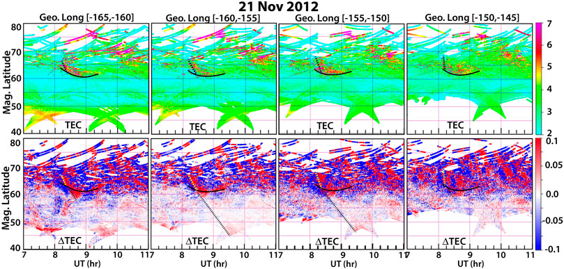
FIGURE 8. Average TEC and ΔTEC over 5° geographic longitude increments from west of, to near, Poker Flat on November 21, 2012 in the same format as Figure 4.

Figures 9, 10 show observations from an event with onset at 1051:15 UT on March 15, 2013. In this case, the onset was west of Poker Flat and a streamer moved into the PFISR FOV as the substorm expansion-phase auroral bulge moved eastward. The flow channel associated with this streamer was seen by both PFISR and SuperDARN from ∼1103 to 1117 UT and was accompanied by an ∼300 nTN-component ground magnetic decrease as seen in Figure 9. Again, a direct connection between the streamer and an equatorward propagating TID can be seen in the ΔTEC panels in Figure 10. While the streamer-related TEC enhancement can be seen in the TEC panels to the equatorward boundary of the auroral oval, fairly intense post-midnight aurora persisted after the streamer within the two more eastern longitude sectors. This led to a few degrees in latitude gap between the TEC enhancement of the streamer and ΔTEC of the TID in those two sectors, with this effect in ΔTEC being the result of the background subtraction using a 30-min sliding average.

FIGURE 9

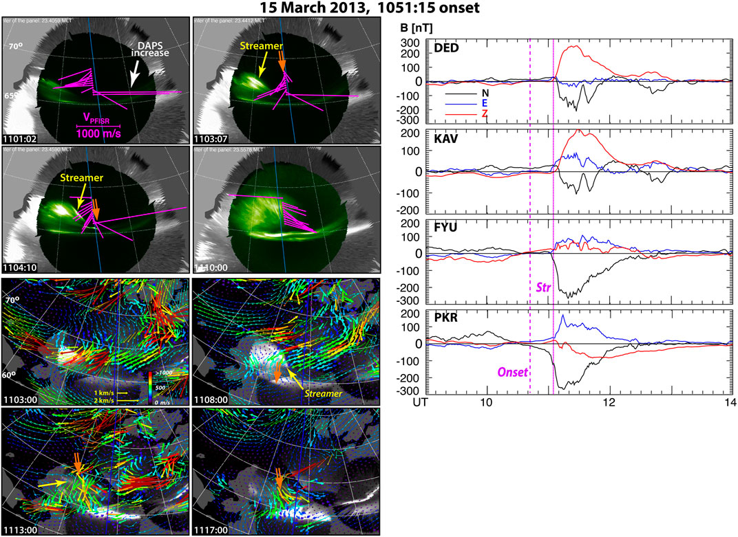
FIGURE 9. Observations on March 15, 2013 during a period when PFISR was operating, and there were sufficient SuperDARN echoes available in regions of interest to provide some two-dimensional flow coverage. Format is the same as Figure 7.

FIGURE 10

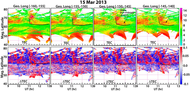
FIGURE 10. Average TEC and ΔTEC over 5° geographic longitude increments from west of, to 5° east of, Poker Flat on March 15, 2017, in the same format as Figure 4.

Figure 11 shows a somewhat more complicated event with onset at 0902:55 UT on March 9, 2013. Onset was to the east of Poker Flat, and, as seen in the 0,909:47 panel. PFISR saw enhanced flows in the SAPS region associated with the westward expansion of the onset brightening and eastward flow toward the head of the oncoming westward traveling surge, as discussed in the study by Lyons et al. (2021b). As identified on the Poker Flat ASI images/ground magnetic field plots on the left/right portion of the figure, three periods of streamers were identified after the surge head moved westward over Poker Flat with ∼100–300 ground N-component magnetic field decreases. Flow enhancements roughly parallel to the local streamer orientation were seen in the PFISR measurements for each as indicated by orange arrows, the enhanced flows being southwestward and just equatorward of the southwestward extending portion of the first streamers, southeastward and just poleward of the southeastward extending portion of one of the second group of streamers, and equatorward with the more north–south–oriented third streamer that was seen through increasingly cloudy skies.

FIGURE 11

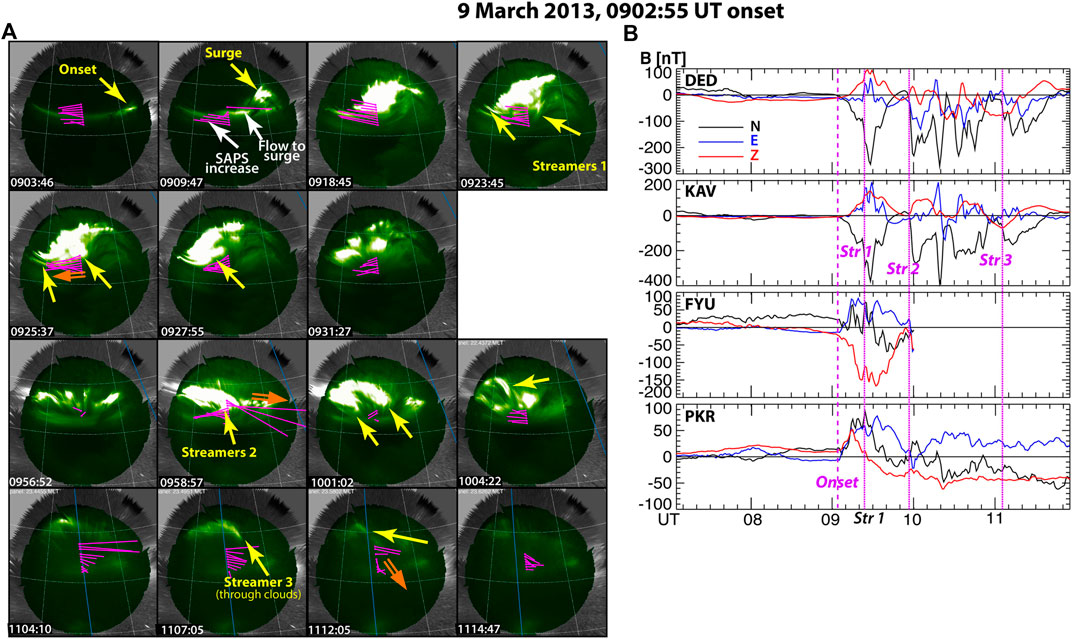
FIGURE 11. Observations on March 9, 2013, during a period when PFISR was operating. (A) Poker Flat ASI 557.7 nm emissions with THEMIS ASI white light emissions in regions outside the Poker Flat ASI FOV overlaid with PFISR flow vectors along the radar magnetic meridian. (B) Ground magnetometer observations from stations approximately along the Poker Flat meridian stacked from lower to higher latitudes. “Str” is abbreviation for “streamer.” Yellow arrows point toward streamers, and orange arrows indicate observed streamer-related flows. Observations from the period before and during the first streamer period are shown in the top two rows, and observations from the second and third streamer period are shown in the third and fourth rows, respectively.

Turning to Figure 12, we can see the ionization from the three sets of streamers more clearly in the ΔTEC panels than in the TEC panels. Each of the streamer-related equatorward moving ΔTEC enhancements can be seen to connect to an equatorward propagating ΔTEC enhancement as indicated by the dashed lines, and thus to a TID at latitudes below the auroral oval. (In a few locations, the ΔTEC transitions, such as that for the first TID in the left column, are from white or light red to deeper red. But these still represent an increase near to somewhat above the 0.03 resolution of the ΔTEC measurements.)

FIGURE 12

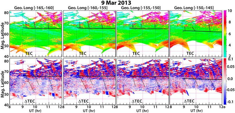
FIGURE 12. Average TEC and ΔTEC over 5° geographic longitude increments from west of, to near, Poker Flat on March 9, 2013, in the same format as Figure 4.

3.3 November 11, 2012, and August 22, 2014: Weak Magnetic Depression

The two examples in Figure 13 have well-defined flow channels as seen in the SuperDARN flow vectors. Two separate flow channels are shown from November 11, 2012, one near 0956 UT and the other near 1030 UT. The flow channels both turn westward around a poleward boundary intensification seen in the aurora images and also eastward in the region of DAPS. The flow channel on August 22, 2014 is shown over a ∼15 min period and quite clearly moved into the auroral oval from the polar cap and turned eastward at Λ ∼65–67° into what is likely the DAPS region. As can be seen by the SuperMAG L index (SML), there were no ground magnetic field decreases exceeding a few tens of nT with these flow channels. While there are some TEC variations as seen within the auroral oval in the ΔTEC panels, there are no discernible equatorward moving regions of ΔTEC below the roughly (due to the weak TEC enhancement from the weak auroral precipitation) estimated equatorward boundary of the auroral oval near the times of the flow channels. (On November 11, 2012, the feature near 10 UT is approximately vertical in the plot, and thus cannot be an equatorward propagating TID. The features at 11 UT, and maybe also at 1130 UT, could be TIDs, but those are well after the time of the flow channels.) This lends support to our previous suggestion (Lyons et al., 2019) that a sufficiently large ionospheric current is necessary for a flow channel to lead to an LSTID, with a few tens of nT ground magnetic field decreases not being sufficient.

FIGURE 13

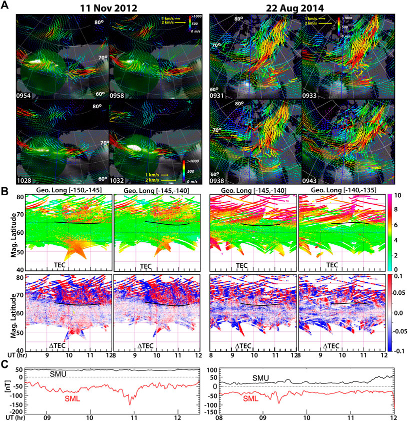
FIGURE 13. Examples having well defined flow channels as seen in the SuperDARN flow vectors. (A) Two separate flow channels are shown from November 11, 2012, one near 0956 UT and the other near 1030 UT and one from August 22, 2014. (B) Average TEC and ΔTEC over 5° geographic longitude increments from near and 5° east of, Poker Flat on the above two dates in the same format as Figure 4, except without dashed lines identifying features. (C) SuperMAG U and L indices (SMU and SML) for the above two dates.

4 Summary and Conclusion

LSTIDs are often viewed as a chain of waves having a period such as the 1.8 h average as in the study by Ding et al. (2008). However, Ding et al. noted that 79% of the events they detected were a single perturbation pulse, suggesting that LSTIDs may be generated impulsively. Consistent with this, the wave periods in their Figure 1 do not show a tendency for an intrinsic period. Instead, the periods are essentially distributed uniformly from ∼0.5 to ∼3 h. This suggests that most LSTIDs are generated impulsively. While Ding et al. only considered storm periods, it is reasonable that this result also applies to non-stormtime conditions. In the present study, we have taken advantage of the existence over Alaska of simultaneous auroral imaging with the Poker Flat and THEMIS ASIs, radar flow measurements with PFISR and SuperDARN, and TEC measurements. This has allowed us to test our previous suggestion that there may be a direct connection of LSTIDs to auroral streamers and associated flow channels having a significant ΔB. Such a connection would indicate that LSTIDs are often generated impulsively by the flow channels and their associated auroral precipitation.

We considered seven nights of observations from our previous studies that had good auroral viewing and clear observations of flow channels and/or streamers. 12 separate relatively ideal events were analyzed, and these events have allowed us to minimize ambiguities in looking for the direct connection of streamers with TIDs. Based on previous studies, TIDs propagating equatorward from the auroral oval in association with auroral zone disturbances are LSTIDs. Thus, the events analyzed here are likely LSTIDs, although we do not have sufficient TEC coverage to demonstrate that the events we observed are indeed large scale.

We started with two nights in 2017 for which the TEC coverage is the best, allowing for two-dimensional images that show the TEC enhancements from streamers and their ensuing connection to TIDs. For the four events on these nights, a longitudinally extended region of TEC enhancement was observed to start to move equatorward from the auroral oval as a group of streamers contacted the equatorward boundary of the oval, thus showing a direct connection covering the approximate range of longitude of the streamers. During the next three nights considered, we saw a direct connection of the streamer-associated ionization and a TID for five events having radar coverage, showing the flow channels associated with the streamers and their connection to TIDs.

For all the above events, these TID regions moved equatorward below the auroral equatorward boundary, and, for each event, the TID region moved at a slower speed than did the TEC enhancements due to the electron precipitation of the associated streamers. These observations indicate that the TID is indeed a different feature from the streamer precipitation. They further indicate that there is a direct connection between the streamers together with their flow channels within the auroral oval and an ensuing TID that propagates equatorward more slowly than does the streamer ionization enhancement. This is consistent with the possibility that heating and momentum transfer from the streamer-related precipitation and flow are responsible for forming the gravity waves that produce the TIDs arising from the nightside auroral-oval, as seen in the flow channel simulations in the study by Deng et al. (2019). Note that we have recently found interesting azimuthal diversion and expansion of flow channels as they approach the equatorward portion of the auroral oval/near-Earth plasma sheet (Wang et al., 2018; Lyons et al., 2021c) that has not yet been included in simulations to determine its effects on TID formation.

All the above events had ground magnetic N-component decreases of a few hundred nT. In contrast, the final two events we examined had clear flow channels in the SuperDARN data but substantially weaker ground magnetic depressions, and a discernible TID was not observed in association with these flow channels. These indicate that a flow channel must lead to a sufficiently large ionospheric current for it to lead to a detectable LSTID, with a few tens of nT ground magnetic field decreases not being sufficient.

Our results give evidence that LSTIDs can be generated impulsively by the flow channels and their associated auroral precipitation, offering a plausible explanation for Ding et al.’s (2008) results that the large majority of LSTID events are a single perturbation pulse. The fact that Ding et al.’s results are available for many events suggests that the impulsive generation by flow channels may be quite common. However, we have examined only 12 events so that further testing of this conclusion is warranted. We note One final point is that we had anticipated that we might see an association between individual flow channels and TIDs. However, we never observed just a single flow channel or streamer. Each of our events consisted of a few streamers and flow channels over a period on the order of 15 min and a longitude range of ∼15–20°. Such groups of streamers are common during substorms. However, to the best of our knowledge, there have not been studies of whether or not streamers and their associated flow channels typically occur in groups.

Data Availability Statement

Publicly available datasets were analyzed in this study. These data can be found here: SuperDARN data are accessible via http://vt.superdarn.org/tiki-index.php?page=Data+AccessSML, and SMU indices used here are available via the SuperMAG at http://supermag.jhuapl.edu/. The University of Alaska ASI data are available at http://optics.gi.alaska.edu/optics/. The THEMIS ASI data are available at http://themis.ssl.berkeley.edu/themisdata/. The PFISR data are available at amisr.com/database and isr.sri.com/madrigal.

Author Contributions

LL: all aspects of the paper; YN: all aspects of the paper; SZ: TEC and TID evaluation; AC: TEC and TID evaluation; WB: SuperDARN radar data analysis; AR: PFISR radar data analysis; RV: PFISR radar data analysis; DH: Poker Flat ASI data analysis. All authors contributed to the article and approved the submitted version.

Conflict of Interest

The authors declare that the research was conducted in the absence of any commercial or financial relationships that could be construed as a potential conflict of interest.

Publisher’s Note

All claims expressed in this article are solely those of the authors and do not necessarily represent those of their affiliated organizations, or those of the publisher, the editors, and the reviewers. Any product that may be evaluated in this article, or claim that may be made by its manufacturer, is not guaranteed or endorsed by the publisher.

Acknowledgments

The study at UCLA has been supported by NSF grants 1907483 and 2055192, NASA grant 80NSSC20K1314 and AFOSR FA9559-16-1-0364, at Boston University by AFOSR FA9559-16-1-0364, NASA NNX17AL22G, NSF AGS-1737823, and AFOSR FA9550-15-1-0179. This material is based upon the study supported by the Poker Flat Incoherent Scatter Radar which is a major facility funded by the National Science Foundation through cooperative agreement AGS-1840962 to SRI International. SuperDARN work at Penn State was supported by AFOSR FA9559-16-1-0364. SuperDARN data are accessible via http://vt.superdarn.org/tiki-index.php?page=Data+Access. SuperDARN is a collection of radars funded by the National Scientific Funding Agencies of Australia, Canada, China, France, Italy, Japan, Norway, South Africa, the United Kingdom, and the United States. Operation of the Kodiak and Adak radars, and processing of the SuperDARN data for this study were supported by the NSF grant AGS1934410 to the University of Alaska Fairbanks. The study at MIT to produce GNSS TEC data products and provide access to them through the Madrigal distributed data system has been supported by the NSF Geospace Facility program under an agreement AGS-1952737. Additional support came from AFOSR FA9559-16-1-0364, NASA LWS funding NNX15AB83G, and AGS-2033787. We thank the SuperMAG and PI Jesper W. Gjerloev for making the ground magnetic field data and SML and SMU indices used here available via the SuperMAG at http://supermag.jhuapl.edu/. The data we have used here are from THEMIS, CARISMA (Mann et al., 2008), the University of Alaska, and USGS (https://www.usgs.gov/natural-hazards/geomagnetism/science/observatories?qt-science_center_objects=0#qt-science_center_objects). The University of Alaska ASI data are available at http://optics.gi.alaska.edu/optics/, and the THEMIS ASI data are available at http://themis.ssl.berkeley.edu/themisdata/. The PFISR data are available at amisr.com/database and isr.sri.com/madrigal.

Supplementary Material

The Supplementary Material for this article can be found online at: https://www.frontiersin.org/articles/10.3389/fspas.2021.738507/full#supplementary-material

References

Azeem, I., Yue, J., Hoffmann, L., Miller, S. D., Straka, W. C., and Crowley, G. (2015). Multisensor Profiling of a Concentric Gravity Wave Event Propagating from the Troposphere to the Ionosphere. Geophys. Res. Lett. 42 (19), 7874–7880. doi:10.1002/2015GL065903

CrossRef Full Text | Google Scholar

Bristow, W. A., Greenwald, R. A., and Samson, J. C. (1994). Identification of High-Latitude Acoustic Gravity Wave Sources Using the Goose Bay HF Radar. J. Geophys. Res. 99 (A1), 319–331. doi:10.1029/93JA01470

CrossRef Full Text | Google Scholar

Bristow, W. A., Hampton, D. L., and Otto, A. (2016). High‐spatial‐resolution Velocity Measurements Derived Using Local Divergence‐Free Fitting of SuperDARN Observations. J. Geophys. Res. Space Phys. 121 (2), 1349–1361. doi:10.1002/2015JA021862

CrossRef Full Text | Google Scholar

Coster, A., Herne, D., Erickson, P., and Oberoi, D. (2012). Using the Murchison Widefield Array to Observe Midlatitude Space Weather. Radio Sci. 47 (6), a–n. doi:10.1029/2012RS004993

CrossRef Full Text | Google Scholar

Coster, A. J., Foster, J. C., and Erickson, P. J. (2003). Monitoring the Ionosphere with GPS. GPS World 14 (5), 42–45.

Google Scholar

Coster, A. J., Goncharenko, L., Zhang, S. R., Erickson, P. J., Rideout, W., and Vierinen, J. (2017). GNSS Observations of Ionospheric Variations During the 21 August 2017 Solar Eclipse. Geophys. Res. Lett. 44 (24), 12041–12048. doi:10.1002/2017GL075774

CrossRef Full Text | Google Scholar

Davis, M. J. (1971). On Polar Substorms as the Source of Large-Scale Traveling Ionospheric Disturbances. J. Geophys. Res. 76 (19), 4525–4533. doi:10.1029/JA076i019p04525

CrossRef Full Text | Google Scholar

Deng, Y., Heelis, R., Lyons, L. R., Nishimura, Y., and Gabrielse, C. (2019). Impact of Flow Bursts in the Auroral Zone on the Ionosphere and Thermosphere. J. Geophys. Res. Space Phys. 124 (12), 10459–10467. doi:10.1029/2019JA026755

CrossRef Full Text | Google Scholar

Ding, F., Wan, W., Liu, L., Afraimovich, E. L., Voeykov, S. V., and Perevalova, N. P. (2008). A Statistical Study of Large-Scale Traveling Ionospheric Disturbances Observed by GPS TEC during Major Magnetic Storms over the Years 2003-2005. J. Geophys. Res. 113 (A3), a–n. doi:10.1029/2008JA013037

CrossRef Full Text | Google Scholar

Francis, S. H. (1975). Global Propagation of Atmospheric Gravity Waves: A Review. J. Atmos. Terrestrial Phys. 37, 1011–1054. doi:10.1016/0021-9169(75)90012-4

CrossRef Full Text | Google Scholar

Frissell, N. A., Baker, J. B. H., Ruohoniemi, J. M., Gerrard, A. J., Miller, E. S., Marini, J. P., et al. (2014). Climatology of Medium-Scale Traveling Ionospheric Disturbances Observed by the Midlatitude Blackstone SuperDARN Radar. J. Geophys. Res. Space Phys. 119 (9), 7679–7697. doi:10.1002/2014JA019870

CrossRef Full Text | Google Scholar

Gallardo-Lacourt, B., Nishimura, Y., Lyons, L. R., Zou, S., Angelopoulos, V., Donovan, E., et al. (2014). Coordinated Superdarn Themis ASI Observations of Mesoscale Flow Bursts Associated with Auroral Streamers. J. Geophys. Res. Space Phys. 119 (1), 142–150. doi:10.1002/2013JA019245

CrossRef Full Text | Google Scholar

Hajkowicz, L. A. (1991). Auroral Electrojet Effect on the Global Occurrence Pattern of Large Scale Travelling Ionospheric Disturbances. Planet. Space Sci. 39 (8), 1189–1196. doi:10.1016/0032-0633(91)90170-F

CrossRef Full Text | Google Scholar

Hayashi, H., Nishitani, N., Ogawa, T., Otsuka, Y., Tsugawa, T., Hosokawa, K., et al. (2010). Large-scale Traveling Ionospheric Disturbance Observed by superDARN Hokkaido HF Radar and GPS Networks on 15 December 2006. J. Geophys. Res. 115 (A6), a–n. doi:10.1029/2009JA014297

CrossRef Full Text | Google Scholar

Hines, C. O. (1960). Internal Atmospheric Gravity Waves at Ionospheric Heights. Can. J. Phys. 38 (11), 1441–1481. doi:10.1139/p60-150

CrossRef Full Text | Google Scholar

Hunsucker, R. D. (1982). Atmospheric Gravity Waves Generated in the High-Latitude Ionosphere: A Review. Rev. Geophys. 20 (2), 293–315. doi:10.1029/RG020i002p00293

CrossRef Full Text | Google Scholar

Jorgensen, A. M., Spence, H. E., Hughes, T. J., and McDiarmid, D. (1999). A Study of omega Bands and Ps6 Pulsations on the Ground, at Low Altitude and at Geostationary Orbit. J. Geophys. Res. 104 (A7), 14705–14715. doi:10.1029/1998JA900100

CrossRef Full Text | Google Scholar

Kubota, M., Fukunishi, H., and Okano, S. (2001). Characteristics of Medium- and Large-Scale TIDs over Japan Derived from OI 630-nm Nightglow Observation. Earth Planet. Sp 53 (7), 741–751. doi:10.1186/BF03352402

CrossRef Full Text | Google Scholar

Liu, J., Lyons, L. R., Wang, C. P., Hairston, M. R., Zhang, Y., and Zou, Y. (2020). Dawnside Auroral Polarization Streams. J. Geophys. Res. Space Phys. 125 (8), e2019JA027742. doi:10.1029/2019JA027742

CrossRef Full Text | Google Scholar

Lyons, L. R. (2000). Geomagnetic Disturbances: Characteristics of, Distinction between Types, and Relations to Interplanetary Conditions. J. Atmospheric Solar-Terrestrial. Phys. 62 (12), 1087–1114. doi:10.1016/s1364-6826(00)00097-3

CrossRef Full Text | Google Scholar

Lyons, L. R., Liu, J., Nishimura, Y., Reimer, A. S., Bristow, W. A., Hampton, D. L., et al. (2021a). Radar Observations of Flows Leading to Substorm Onset Over Alaska. J. Geophys. Res. Space Phys. 126 (2), e2020JA028147. doi:10.1029/2020JA028147

CrossRef Full Text | Google Scholar

Lyons, L. R., Liu, J., Nishimura, Y., Wang, C. P., Reimer, A. S., Bristow, W. A., et al. (2021b). Radar Observations of Flows Leading to Longitudinal Expansion of Substorm Onset Over Alaska. J. Geophys. Res. Space Phys. 126 (2), e2020JA028148. doi:10.1029/2020JA028148

CrossRef Full Text | Google Scholar

Lyons, L. R., Nishimura, Y., Donovan, E., and Angelopoulos, V. (2013). Distinction between Auroral Substorm Onset and Traditional Ground Magnetic Onset Signatures. J. Geophys. Res. Space Phys. 118 (7), 4080–4092. doi:10.1002/jgra.50384

CrossRef Full Text | Google Scholar

Lyons, L. R., Nishimura, Y., Wang, C.-P., Liu, J., and Bristow, W. A. (2021c). Two-Dimensional Structure of Flow Channels and Associated Upward Field-Aligned Currents: Model and Observations. Front. Astron. Space Sci. 8, 143. doi:10.3389/fspas.2021.737946

CrossRef Full Text | Google Scholar

Lyons, L. R., Nishimura, Y., Zhang, S. R., Coster, A. J., Bhatt, A., Kendall, E., et al. (2019). Identification of Auroral Zone Activity Driving Large‐Scale Traveling Ionospheric Disturbances. J. Geophys. Res. Space Phys. 124 (1), 700–714. doi:10.1029/2018JA025980

CrossRef Full Text | Google Scholar

Mann, I. R., Milling, D. K., Rae, I. J., Ozeke, L. G., Kale, A., Kale, Z. C., et al. (2008). The Upgraded CARISMA Magnetometer Array in the THEMIS Era. Space Sci. Rev. 141 (1–4), 413–451. doi:10.1007/s11214-008-9457-6

CrossRef Full Text | Google Scholar

Mende, S. B., Harris, S. E., Frey, H. U., Angelopoulos, V., Russell, C. T., Donovan, E., et al. (2008). The THEMIS Array of Ground-Based Observatories for the Study of Auroral Substorms. Space Sci. Rev. 141 (1–4), 357–387. doi:10.1007/s11214-008-9380-x

CrossRef Full Text | Google Scholar

Nicolls, M. J., and Heinselman, C. J. (2007). Three-dimensional Measurements of Traveling Ionospheric Disturbances with the Poker Flat Incoherent Scatter Radar. Geophys. Res. Lett. 34 (21). doi:10.1029/2007GL031506

CrossRef Full Text | Google Scholar

Nishimura, Y., Lyons, L. R., Kikuchi, T., Angelopoulos, V., Donovan, E., Mende, S., et al. (2012). Formation of Substorm Pi2: A Coherent Response to Auroral Streamers and Currents. J. Geophys. Res. 117, a–n. doi:10.1029/2012JA017889

CrossRef Full Text | Google Scholar

Nishimura, Y., Lyons, L. R., Zou, S., Xing, X., Angelopoulos, V., Mende, S. B., et al. (2010). Preonset Time Sequence of Auroral Substorms: Coordinated Observations by All-Sky Imagers, Satellites, and Radars. J. Geophys. Res. 115, a–n. doi:10.1029/2010JA015832

CrossRef Full Text | Google Scholar

Ogawa, T., Balan, N., Otsuka, Y., Shiokawa, K., Ihara, C., Shimomai, T., et al. (2002). Observations and Modeling of 630 Nm Airglow and Total Electron Content Associated with Traveling Ionospheric Disturbances over Shigaraki, Japan. Earth Planet. Sp 54 (1), 45–56. doi:10.1186/BF03352420

CrossRef Full Text | Google Scholar

Richmond, A. D. (1978). Gravity Wave Generation, Propagation, and Dissipation in the Thermosphere. J. Geophys. Res. 83 (A9), 4131–4145. doi:10.1029/JA083iA09p04131

CrossRef Full Text | Google Scholar

Richmond, A. D. (1979). Large-amplitude Gravity Wave Energy Production and Dissipation in the Thermosphere. J. Geophys. Res. 84 (A5), 1880–1890. doi:10.1029/JA084iA05p01880

CrossRef Full Text | Google Scholar

Rideout, W., and Coster, A. (2006). Automated GPS Processing for Global Total Electron Content Data. GPS Solut 10 (3), 219–228. doi:10.1007/s10291-006-0029-5

CrossRef Full Text | Google Scholar

Saito, A., Fukao, S., and Miyazaki, S. (1998). High Resolution Mapping of TEC Perturbations with the GSI GPS Network over Japan. Geophys. Res. Lett. 25 (16), 3079–3082. doi:10.1029/98GL52361

CrossRef Full Text | Google Scholar

Savitzky, A., and Golay, M. J. E. (1964). Smoothing and Differentiation of Data by Simplified Least Squares Procedures. Anal. Chem. 36 (8), 1627–1639. doi:10.1021/ac60214a047

CrossRef Full Text | Google Scholar

Shiokawa, K., Lu, G., Otsuka, Y., Ogawa, T., Yamamoto, M., Nishitani, N., et al. (2007). Ground Observation and AMIE-TIEGCM Modeling of a Storm-Time Traveling Ionospheric Disturbance. J. Geophys. Res. 112 (A5), a–n. doi:10.1029/2006JA011772

CrossRef Full Text | Google Scholar

Shiokawa, K., Otsuka, Y., Ogawa, T., Balan, N., Igarashi, K., Ridley, A. J., et al. (2002). A Large-Scale Traveling Ionospheric Disturbance during the Magnetic Storm of 15 September 1999. J. Geophys. Res. 107 (A6), SIA 5-1–SIA 5-11. doi:10.1029/2001JA000245),

CrossRef Full Text | Google Scholar

Tsugawa, T., Otsuka, Y., Coster, A. J., and Saito, A. (2007). Medium-scale Traveling Ionospheric Disturbances Detected with Dense and Wide TEC Maps over North America. Geophys. Res. Lett. 34 (22). doi:10.1029/2007GL031663

CrossRef Full Text | Google Scholar

Tsugawa, T., Saito, A., and Otsuka, Y. (2004). A Statistical Study of Large-Scale Traveling Ionospheric Disturbances Using the GPS Network in Japan. J. Geophys. Res. 109 (A6). doi:10.1029/2003JA010302

CrossRef Full Text | Google Scholar

Vierinen, J., Coster, A. J., Rideout, W. C., Erickson, P. J., and Norberg, J. (2016). Statistical Framework for Estimating GNSS Bias. Atmos. Meas. Tech. 9 (3), 1303–1312. doi:10.5194/amt-9-1303-2016

CrossRef Full Text | Google Scholar

Wang, C. P., Gkioulidou, M., Lyons, L. R., and Wolf, R. A. (2018). Spatial Distribution of Plasma Sheet Entropy Reduction Caused by a Plasma Bubble: Rice Convection Model Simulations. J. Geophys. Res. Space Phys. 123 (5), 3380–3397. doi:10.1029/2018JA025347

CrossRef Full Text | Google Scholar

Zakharenkova, I., Astafyeva, E., and Cherniak, I. (2016). GPS and GLONASS Observations of Large-Scale Traveling Ionospheric Disturbances during the 2015 St. Patrick's Day Storm. J. Geophys. Res. Space Phys. 121 (12), 12138–12156. doi:10.1002/2016JA023332

CrossRef Full Text | Google Scholar

Zhang, S. R., Coster, A. J., Erickson, P. J., Goncharenko, L. P., Rideout, W., and Vierinen, J. (2019b). Traveling Ionospheric Disturbances and Ionospheric Perturbations Associated With Solar Flares in September 2017. J. Geophys. Res. Space Phys. 124 (7), 5894–5917. doi:10.1029/2019JA026585

CrossRef Full Text | Google Scholar

Zhang, S. R., Erickson, P. J., Coster, A. J., Rideout, W., Vierinen, J., Jonah, O., et al. (2019a). Subauroral and Polar Traveling Ionospheric Disturbances During the 7-9 September 2017 Storms. Space Weather 17 (12), 1748–1764. doi:10.1029/2019SW002325

CrossRef Full Text | Google Scholar

Zhang, S. R., Erickson, P. J., Goncharenko, L. P., Coster, A. J., Rideout, W., and Vierinen, J. (2017). Ionospheric Bow Waves and Perturbations Induced by the 21 August 2017 Solar Eclipse. Geophys. Res. Lett. 44 (24), 12067–12073. doi:10.1002/2017GL076054

CrossRef Full Text | Google Scholar