Automated bow shock and magnetopause boundary detection with Cassini using threshold and deep learning methods

1 Introduction

Cassini was the first spacecraft to orbit around Saturn’s near-space environment. The mission lasted 13 years (2004–2017) producing the first large-scale in situ dataset at Saturn, returning a total of 635 GB of scientific data (NASA Jet Propulsion Laboratory, 2017). The high spatio-temporal resolution data of the planet and its space environment could be leveraged by data science techniques, including machine learning, to aid the study of outer planets physics.

An ongoing challenge in the study of planetary boundaries like the bow shock (BS) and magnetopause (MP) is their manual identification in big multi-instrument datasets from space missions. From a data analysis perspective, automation of this activity would improve reproducibility, discovery potential in existing unlabelled data, and reusability in existing and future planetary missions. “Human-in-the-loop” scientists combined with partial automation would speed up data selection by orders of magnitude as most data would be pre-classified to a good level of accuracy, whilst only correcting a manageable number of misclassifications would be needed. Automation would facilitate larger crossing lists to be compiled and could also have implications for the future development of onboard data-processing protocols in the pre-downlink stage. From a fundamental perspective, a more complete boundary survey provides an invaluable dataset with which to understand the boundary structures, like the distribution of radial distances, local times, and latitudes at which the boundaries are detected, under different phases of the solar cycle throughout the mission lifetime. This offers a wealth of information about the interface between the planet and the solar wind.

In recent years, there have been multiple studies on the application of machine learning techniques, including deep learning, to automate the process of selecting or detecting plasma regions or boundaries from spacecraft data, many of which focus on space missions of the Earth, with a few for other planets such as Saturn. Recent studies which used Earth space mission data include: Automating the detection of the Earth’s bow shock (BS) and magnetopause (MP) using gradient boosted decision trees (Nguyen et al., 2019), automating the burst data selection process onboard the MMS spacecraft using a Long-Short Term Memory (LSTM) Recurrent Neural Network (RNN) model (Argall et al., 2020), automating the classification of plasma regions in near-Earth space using a time series convolutional model on engineered features from MMS data (Breuillard et al., 2020), automating region identification in MMS data using support-vector-machines in the density and temperature (n-T) space (da Silva et al., 2020), automatically classifying plasma regions using convolutional neural networks on three-dimensional ion energy spectra produced by DIS sensor onboard MMS (Olshevsky et al., 2021), and predicting plasma regimes and thermal electron density from WHISPER spectra onboard Cluster II using neural networks Gilet et al. (2021). Recent studies which used Saturn space mission data include a threshold-based detection of boundary crossings at Saturn from Cassini’s plasma spectrometer data using a transition detection score (Daigavane et al., 2022), and automatic plasma region classification using an RNN model on Cassini time-series data (Yeakel et al., 2022).

Despite the recent interest in using machine learning models to tackle the problem of automating such pattern recognition tasks in spacecraft data, more traditional methods such as using thresholds of different engineered parameters have been used to identify potential plasma boundaries such as in Case and Wild (2013) in which they compared MP modelled positions and in situ Cluster data. However, each space mission provides its unique challenges.

This study aims to develop and compare traditional threshold and deep learning techniques to automate the detection of the bow shock and magnetopause boundary crossings at Saturn using data from the Cassini spacecraft. The potential to apply such techniques to other planetary boundary studies is also discussed.

1.1 Deep learning models

The following section gives a brief introduction to the deep learning models used in this study for context. Neural networks are powerful function approximators. A feed-forward deep neural network contains two or more layers of neurons. Mathematically, each layer applies a linear operation to its input according to z = WX + b, where W and b are the weights and biases (i.e., learned parameters) of that layer, and X is the input. The output z is then “activated” by an activation function. The activation is a non-linear function, such as the Rectified Linear Unit (ReLU) f(z) = max (0, z), applied to the output of a layer to introduce non-linearity. In short, a fully connected neural network performs the following operations: “weight times input, add a bias, activate”. A trained neural network with learned parameters represents the best function approximation which defines the mapping y = f (x; W, b) (Goodfellow et al., 2016).

1.1.1 Autoencoder

The autoencoder (AE) is an unsupervised learning neural network architecture trained to reconstruct the input as close as possible from a compressed latent space (i.e., the network learns to map an input X to an output X). This dimensionality reduction capability of an AE has been demonstrated by Hinton and Salakhutdinov (2006). The AE architecture contains two parts, an encoder (g_ϕ) and a decoder (f_θ). The encoder block takes an input (e.g., an image or sequential data) and compresses it to a latent vector z, then the decoder block learns to reconstruct the input from the compressed representation. The training of the AE neural network involves using backpropagation (i.e., chain rule) to minimise the following loss function

$L_{AE}\left(\theta ,\varphi ,x\right)=\sum _n\left(x_n-f_{\theta }{\left(g_{\varphi }\left(x_n\right)\right)}^2\right.,(1)$

with respect to the network parameters (θ, ϕ) to output a reconstructed data sample as close as possible to the original input x ≈ f_θ(g_ϕ(x)). The loss function in Eq. 1 is the sum of the squared error between the input and output. For sequential data, the encoder and decoder blocks utilise a long short-term memory (LSTM) recurrent neural network, which is adept at learning longer-term dependencies in time-series data due to their “memory cell” function. For more details, refer to Sak et al. (2014).

The motivation for the use of an AE was that boundary crossings usually contain turbulent magnetic fields on the magnetosheath side, whilst the majority of the intervals in the magnetosphere and solar wind contain smoother magnetic field profiles. It is expected that the AE would reconstruct the magnetosheath fields worst, compared to magnetospheric or solar wind fields. Thus, this feature could be leveraged to identify potential regions of crossings between distinct plasma regions.

1.1.2 Residual convolutional neural network (ResNet)

A plain Convolutional Neural Network (CNN) is typically used in a supervised learning setting like image classification. Convolution involves sliding a ‘kernel’ over an image to extract certain ‘features’ from the image to identify the class to which it belongs. Each layer in a CNN extracts a different level of features of the input image based on the kernel parameters. Eventually, the input image becomes a latent vector of a single dimension (similar to the output of the encoder part of the autoencoder 1.1.1). This latent vector is finally passed through a fully connected neural network in order to output a classification. In traditional image classification, these ‘kernels’ are hand-engineered. However, CNN automatically learns features in the image through gradient-based learning (LeCun et al., 1999) using backpropagation (i.e., chain rule) to minimise the following loss function

$L\left(y,\mathrm{t}\mathrm{r}\mathrm{u}\mathrm{e}\mathrm{c}\mathrm{l}\mathrm{a}\mathrm{s}\mathrm{s}\right)=W_{\text{true\hspace{0.17em}class}}\left(-\log \frac{\exp \left(y_{\text{true\hspace{0.17em}class}}\right)}{{\sum }_j\exp \left(y_j\right)}\right)(2)$

with respect to the parameters of the kernels, where y is the output vector from the final layer of the network with dependence on network parameters, whose length is the same as the number of classes in the classification problem, trueclass specifies the index of the element in y corresponding to the true class, and W_{true class} is the weight of the true class. These class weights are particularly useful when the dataset contains a strong class imbalance such that bigger weights could be applied to minority classes to improve their classification performance. This loss function is called the cross entropy loss which combines the negative log function with the softmax function (the arguments inside the log). To minimise this loss, the network parameters are adjusted based on the gradients such that the element of y which corresponds to the true class becomes larger. In other words, the smallest loss is achieved when the numerator in Eq. 2 is largest (i.e., the network predicts the true class with a high probability), whilst the biggest loss is seen when the numerator is smallest (i.e., the network predicts the true class with a low probability).

Deeper neural networks (i.e., more layers of neurons) can generally perform more complex mappings due to more tunable parameters. However, very deep neural networks are difficult to train due to the vanishing gradient problem in which gradients of the loss function with respect to the network parameters are close to zero and the network cannot minimise the loss function further (Goodfellow et al., 2016). The ResNet architecture developed by He et al. (2016) overcomes this by introducing ‘skipped connections’ which allowed successful training of deep neural networks. ‘Skipped’ connections are where the activation from one layer is directly added to another layer deeper in the network, as shown in Figure 1. This allows a deep neural network to continue tuning the parameters of the network to minimise the loss function and improve its classification performance. Mathematically, the skip-connections of a residual block are combined with L2-regularisation (i.e., a penalty term to minimise the values of the learnable parameters) and ReLU activation function, to allow for zero weights and biases for the extra (potentially redundant) layer of neurons in the network leading to zero contribution from this added layer, thus giving the residual block the ability to learn the identity function easily. That is to say, the activated output of the added layer is the same as the activated output of some previous layer connected by the skipped connection. Therefore, deeper networks with residual blocks do not hinder the learning ability of the overall network compared to shallower networks because it is easy for the residual block to produce the same output as prior to adding the extra layers.

FIGURE 1

FIGURE 1. A residual learning block as illustrated in He et al. (2016). In this schematic, there are two convolutional layers acting on the input (x) followed by an element-wise summation operation with x via the ‘skipped’ connection.

The motivation for using the CNN for boundary detection came from how the existing catalogue of crossings was created. The data were manually surveyed by human eyes looking for characteristic features of BS and MP as described in Section 2.2.1. This bodes well for automation with computer vision models due to the visual distinctive features seen in the plots of the data.

2 Materials and methods

The life-cycle for this project consisted of four main stages: 1) Scoping, where the project goal is defined. 2) Data, where the data source is defined, the pre-processing steps are established, the features and labels for the events of interest are defined, and a baseline performance is established (e.g., human-level performance for boundary classification). 3) Modelling, where the data is modelled with different algorithms and performing error analysis to understand areas of improvement both with the models’ parameters and also the data itself, 4) Deployment, where the system is used on new data and is monitored and maintained to ensure proper functioning. The algorithm implementations were done in Python and the deep learning models were built using the PyTorch framework (Paszke et al., 2019).

2.1 Scoping

The task of boundary detection can be broadly framed as a classification problem. Therefore, the scope of this project is to build an automated system that, given an interval of magnetic field and plasma data, outputs a list of candidate times corresponding to bow shock (BS) and magnetopause (MP) crossings.

2.2 Data

For this study, magnetic field and particle data from Cassini were used to detect BS and MP crossings. These measurements were obtained by the following two instruments on board Cassini: The dual-technique magnetometer (MAG) (Dougherty et al., 2004), and the electron spectrometer (ELS) part of the CAPS (Cassini Plasma Spectrometer) instrument (Young et al., 2004). MAG provided the magnetic field measurements from which 1-min averaged data were used. The coordinate system was Kronocentric solar magnetospheric (KSM), where X points from the centre of Saturn to the Sun, Y points in the direction Ω × X (where Ω is Saturn’s rotational/magnetic dipole axis), and Z completes the right-handed coordinate system. Moments derived from 8-s averaged distributions in the ELS data provide electron density and temperature. The ELS instrument has eight anodes which sweep through 63 bins covering an energy range of 0.6 eV–28.25 keV in 2 s. The ELS is able to detect electron density as low as $\sim 10^3{\mathrm{m}}^{-\mathrm{3}}$ (Young et al., 2005). The field of view of each anode is 20° × 5° (thus 160° × 5° for all eight anodes). An actuator rotates the anodes back and forth covering $\sim 2\pi$ sr of solid angle. The coverage may be increased if the spacecraft is rolling. For this study, we used anode 5 for all electron measurements as it has relatively large pitch angle coverage (angle of electron velocity relative to the local magnetic field) throughout an actuation cycle, compared to other anodes.

Cassini provided 13 years of data from 2004 to 2017. The latest catalogue of crossings at Saturn produced by Jackman et al. (2019) consisted of 2,118 MP crossings and 1,243 BS crossings, both of which were recorded as single timestamps, and were identified mainly using 1-min MAG data, but validated with CAPS electron data when available.

2.2.1 BS and MP crossing features

For the creation of the boundary crossing list, a range of visual characteristics can be seen in the MAG and CAPS datasets.

Bow shock (BS) crossings have the most distinct features in both MAG and CAPS data. It involves transitioning between solar wind (SW) on one side and magnetosheath (SH) on the other. The SW exhibits a quiet, low-magnitude interplanetary magnetic field (IMF) and relatively cold electrons ($\le 10$ eV). In contrast, the magnetosheath exhibits turbulent, enhanced IMF with typical field fluctuations such as mirror mode compressions (Joy et al., 2006) (which are often excited under sheath-like conditions) and heated ion and electron energy spectra ($\le 100$ eV). A spacecraft moving from SW into SH will often measure a clear increase in magnetic field strength, typically accompanied by a magnetic ‘overshoot’ (Achilleos et al., 2006). In occasional cases where the magnetic features were unclear for a BS crossing (e.g., a rapid pair of BS crossings occurred around 2012-04-01 03:00:001), CAPS data would typically display a sharp change in both density and temperature of the plasma at BS crossings, see Figure 2 for examples. Sulaiman et al. (2016) have shown that the magnetic overshoot is strongly correlated with the Alfvén Mach Number (M_A) which depends on upstream field strength and solar wind dynamic pressure. The authors also point out that Saturn has the largest range of M_A due to the highly variable upstream conditions, which could explain the large variety of BS crossing appearances in the data.

FIGURE 2

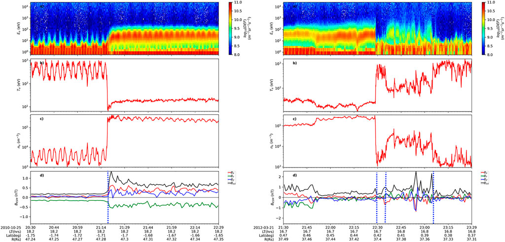
FIGURE 2. Example bow shock crossings (marked by vertical blue dotted lines). The panels are: (A) Electron energy-time spectrogram of differential energy flux (DEF) from CAPS/ELS anode 5. (B,C) Electron temperature and number density derived from ELS anode 5. (D) The magnitude and KSM components of the magnetic field, with bow shock crossings marked by vertical blue dotted lines. Spacecraft ephemeris data are given below the x-axis of the plots. Note that the derived electron moments within the solar wind are invalid so should not be considered.

Magnetopause (MP) crossings can be identified by both a change in the nature of fluctuations and the direction of the magnetic field, such as those found on the Earth [e.g., Phan et al. (2013); Phan et al. (2014)], and similar features are observed at Saturn. For inbound MP crossings, the field typically changes from the more turbulent fluctuations in the magnetosheath to the steadier field in the magnetosphere, accompanied by a rotation of the field to a southward (magnetospheric) orientation, and increased field strength. However, there may be cases where magnetosheath fields may not be turbulent (with a small standard deviation) such as during the MP encounters between 2005-08-15 12:00:00 to 2005-08-15 20:00:00 (Supplementary Figure S1). Furthermore, MP crossings with low magnetic shears (small change in field orientation across the MP) as found by Masters et al. (2012) may also be ambiguous using MAG data alone. In such cases, CAPS data would generally show a change from the steady electron energy spectra of the magnetosheath (higher density, lower temperature electrons) to the more variable magnetospheric populations (lower density, higher-temperature electrons), see Figure 3 for examples.

FIGURE 3

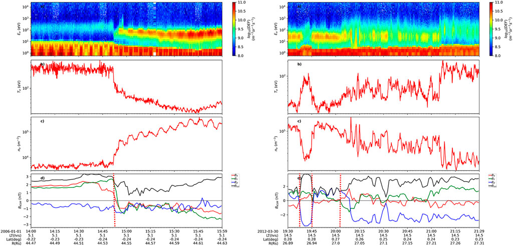
FIGURE 3. Example magnetopause crossings (marked by vertical red dotted lines). The panels are: (A) Electron energy-time spectrogram of differential energy flux (DEF) from CAPS/ELS anode 5. (B,C) Electron temperature and number density derived from ELS anode 5. (D) The magnitude and KSM components of the magnetic field, with bow shock crossings marked by vertical blue dotted lines. Spacecraft ephemeris data are given below the x-axis of the plots.

Typical speeds of Saturn’s magnetopause are of order 100 km/s (Masters et al., 2011), which is of the same order as the estimated speed of Saturn’s bow shock (Achilleos et al., 2006). For typical MP crossings of duration between 5-min to 10-min, this gives a thickness of roughly 0.5 to 1 R_S (Saturn radii), or equivalent to $\sim 25$ to $\sim 50$ magnetosheath proton gyroradii (based on typical E = 100 eV, B = 1 nT), which is of the same order as the estimated MP thickness of $\sim 10$ thermal proton gyroradii at Earth (e.g., Le and Russell 1994). Typical magnetosheath electrons (E = 100 eV, B = 1 nT) have a gyroradius of r_ge ≈ 30 km which is more than three orders of magnitude smaller than the typical width of the MP current layer. Given a boundary that is much thicker than typical electron gyroradii, and that the MP is closed (i.e., no magnetic connectivity between magnetosheath and magnetosphere), electrons are usually unable to cross the MP boundary but instead flow tailward (downstream towards Saturn nightside) along the magnetosheath field lines. Thus, the MP current sheet separates well the magnetosheath electrons and magnetospheric thermal electrons at energies close to the modal energy. Despite this natural separation of electron populations by the MP boundary, test particle simulations by Kim and Lee (2014) have shown that higher energy electrons from the Earth’s outer radiation belt can escape through a closed MP into the magnetosheath via gradient drift. They showed that the weaker the B-gradient, the higher the energy of electrons is required to escape into the magnetosheath: E.g., for a magnetic field gradient scale length of ∼ 17 R_E along the magnetopause, the minimum kinetic energy for loss is ∼ 3 MeV. The large variety of MP crossings is likely due to the different plasma processes and evolving structures which may occur at the MP boundary such as electron heating associated with magnetic reconnection (McAndrews et al., 2008; Cheng et al., 2021), Kelvin-Helmholtz vortices, (Masters et al., 2010), plasma depletion layers (Masters et al., 2014) and low-latitude boundary layers (Masters et al., 2011).

2.2.2 Data preprocessing

The preprocessing pipeline provides a systematic way to process large spacecraft datasets for data-driven modelling.

The first part of data-preprocessing involved reducing the search scope for BS and MP boundary crossings. Sections of Cassini’s orbits were pre-selected based on the conservative estimates of the minimum and maximum standoff distances for the BS and MP boundaries (i.e., distance from the centre of Saturn to the subsolar point of the MP or BS). These standoff distances were found by fitting empirical models for BS (Went et al., 2011) and MP (Pilkington et al., 2015) surfaces to pass through Cassini’s positions. Note that the polar flattening and dawn-dusk asymmetry coefficients from the Pilkington model were not used here (i.e., the assumed MP surface was axis-symmetric). The same fitting was done to the catalogue of crossings. From this result, the minimum and maximum nose standoff distances used for MP were 13 and 43 R_S respectively, and the shock standoff distances were 16 and 51 R_S respectively. These values were used to select orbital segments which captured all of the crossings in the catalogue. This produced a list of intervals with a cumulative total time of 4,178,770 min (∼ 8 years) out of the 13-year mission.

To further reduce the search space, the second preprocessing part used an autoencoder (AE) for unsupervised outlier detection. The input magnetic field vector values were scaled to between 0 and 1 for the purpose of training the neural network. The scaling is given by:

$X_{\mathit{scaled}}=\frac{X-\mathrm{m}\mathrm{i}\mathrm{n}\left(X\right)}{\mathrm{m}\mathrm{a}\mathrm{x}\left(X\right)-\mathrm{m}\mathrm{i}\mathrm{n}\left(X\right)}(3)$

where X is the quantity of interest such as the magnetic field, min and max are the minimum and maximum of the quantity respectively, over the pre-selected intervals of data. The autoencoder algorithm has been used in other space physics applications such as finding anomalies in electron distribution functions (Bakrania et al., 2020). Since the data were sequential, the layers of the AE consisted of long short-term memory (LSTM) units (Sak et al., 2014). The dataset included windows of magnetic field data constructed from the pre-selected orbital segments from the first part of data-preprocessing. The sequence length for each window was 60 min at 1-min resolution, and the stride was set to 30 min. After removing the windows which contained missing data or ‘NaN’, the resulting shape of the dataset was (125553, 60, 4) where 125,553 was the total number of windows of magnetic field data, 60 was the sequence length, and 4 represented B_x, B_y, B_z and |B| (i.e., the three field components in KSM coordinates and the field magnitude).

After training the network with the adam optimiser (Kingma and Ba, 2015) (which is suited for optimising systems with lots of parameters like neural networks), it was found that the AE was able to reconstruct the smooth persistent changes of each magnetic field component, however not the local smaller scale fluctuations. Field profiles containing rapid, large-amplitude fluctuations, or field rotations in one or more components, tended to have higher reconstruction loss. By calculating the median loss value for the entire dataset of 60-min intervals, it was used as a threshold to accept or reject each interval for potential boundary crossings. Figure 4 shows the reconstruction loss for the pre-selected intervals in 2016. Generally, it was found that intervals with high loss values were mostly associated with magnetosheath regions as expected, but also associated with most BS and MP crossings. In contrast, pure magnetospheric and solar wind intervals have relatively smoother field profiles and thus lower loss values.

FIGURE 4

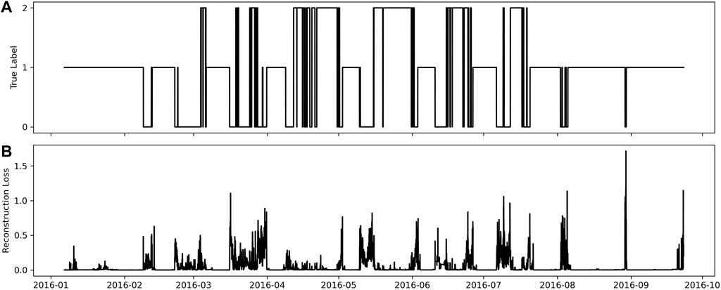
FIGURE 4. LSTM autoencoder network predictions for test magnetic field timeseries data in 2016. (A) True region labels based boundary crossing list. The labels SH, SP, SW are magnetosheath, magnetosphere and solar wind, respectively. (B) Magnetic field profile reconstruction loss.

The result of this step reduced the search space by 49% whilst retaining 97% of crossings in the latest catalogue (Jackman et al., 2019). For comparison, standard scaling (zero mean and unit variance) was applied to the same dataset to select windows of magnetic field profiles which had at least a single field component with a Z-score greater than three (i.e., three standard deviations from the mean of the 60-min interval). This method of filtering reduced the amount of data to search by 38% whilst only retaining 80% of crossings in the catalogue. This indicated that the LSTM AE method could offer more flexibility regarding outlier detection of sequential data.

2.2.3 Train, validation and test dataset

Figure 5 compares the BS and MP crossings between 2004 to 2012 and 2013 to 2016. It is apparent that many of the 2013–2016 crossings had much higher planetary latitudes than those between 2004–2012. This was due to increasingly higher inclination orbits towards the end of the mission, allowing Cassini to sample the magnetosphere at much higher latitudes. Around 80% of the crossings in the catalogue were found before the CAPS instrument was turned off, and 20% after it was switched off (between 2012-06-02 to the end of the mission in September 2017). It is crucial for learning algorithms to have consistent labels to train from because a noisy mapping between input data and output labels may lead to poor convergence towards the true underlying function. For traditional programmatic algorithms where rules are hard-coded, it is equally important to have a reliable ground truth dataset for evaluating the performance of the algorithmic detections.

FIGURE 5

FIGURE 5. The positions of BS and MP crossings as observed by Cassini. (A) 2004–2012 was when CAPS data were largely available, and the orbits covered all of pre-equinox, equinox and 2 years of the solstice mission. (B) 2013–2016 was when only MAG data were available, which covered the remaining part of the solstice mission.

The decision was thus made to train on data between 2004–2011 whilst the first half of the 2012 data were used for testing the algorithms, as validation with CAPS data was expected to produce more consistent crossing labels. For the remainder of the data, between 2012–06 to 2016-08, where crossings did not have CAPS data for validation, a MAG-only detection model was used.

For the CNN model, initially, the scope was simplified to a binary classification problem: Does the input interval contain a crossing or not? It was later modified to perform multiclass classification with classes ‘notCrossing’, ‘BS’, and ‘MP’. The CAPS and MAG data were prepared according to the following procedure. A list of 2-h time intervals with 30-min strides was produced. The magnetic field plot images had a fixed y-scale ranging from −10 nT to 10 nT. The CAPS-ELS spectrogram images had a fixed y-scale ranging from 0.6 eV to 28.25 keV in logarithmic scale consisting of the 63 energy bins of the CAPS ELS instrument. An illustration of both types of images is shown in Figure 8. This provided a dataset of 73,623 images of MAG and CAPS-ELS plots in total between the years 2004–2012. The class distribution for these images were: 66,513 (90%) notCrossing, 4,994 (7%) MP and 2,116 (3%) BS. This strong class imbalance was addressed by using class weights during model training as described in the cross entropy loss function (Eq. 2). The years used for training and validating the CNN were 2004–2011 with an 80:20 split respectively. A stratified splitting was used in which the data were shuffled to ensure that the class ratios were preserved in both the train and validation dataset. A histogram of the time intervals between consecutive crossings and a distribution of crossing epochs (on the Cassini mission timeline) for both the train and validation dataset are included in the Supplementary Material (Supplementary Figures S3, S4). For the test dataset, the remaining 2012 data with CAPS available were used. The nature of time-series data means that the train and test data should not be shuffled together. From a physical point of view, the equinox (2012) structure of Saturn’s current sheet and magnetosphere is quite distinct from that of distantly pre-equinox times (e.g., summer solstice). Hence an algorithm which performs effectively under this constraint would certainly be expected to perform just as well, if not better when applied to test cases drawn from the pre-equinox mission epoch. Using the results from the autoencoder data-preprocessing stage, the 2-h intervals from the training dataset were discarded if the corresponding interval of magnetic fields could be recreated with better than median reconstruction loss (i.e., a lower loss value) as they would likely not contain a crossing. This reduced the number of training images to 37,057.

To derive the final list of crossings, the start time of the first positive detection and the end time of the last positive detection was extracted from continuous positive detections of the 2-h windows. This ensured that the interval contained the crossing of interest. A single timestamp of the crossing could be estimated by taking the centre of the interval, but precise timings would still need to be extracted manually. In terms of spacecraft position, this interval is usually short enough that it appears as a single point in a typical spatial plot. However, this method of producing a final list of crossing times depended on the assumption that individual crossings were separated by a sufficient time such that consecutive 30-min strides would not continuously yield positive detections allowing the chain of positive detections to be broken, but this was not always the case.

2.3 Modelling

The next step in the pipeline was the modelling part in which algorithms were designed to perform the BS and MP classification in order to re-discover the catalogue of crossings.

Two different types of models were implemented to detect and classify boundary crossings. The performance of traditional threshold and modern deep learning techniques was compared to show the strengths and weaknesses of each (Section 3.1).

2.3.1 Threshold method

The threshold method was motivated by a similar use case to automate magnetopause detections at Earth (Case and Wild, 2013). Figure 6 (left) shows the magnetic field data with four field parameters for thresholding (bottom two panels). On the right, CAPS electron data is shown with four parameters based on density and temperature moments for thresholding (bottom two panels). MAG and CAPS parameter values were computed using two sliding windows of length 30-min with a fixed gap of 8 min in between (shown by the red squares in Figure 6).

FIGURE 6

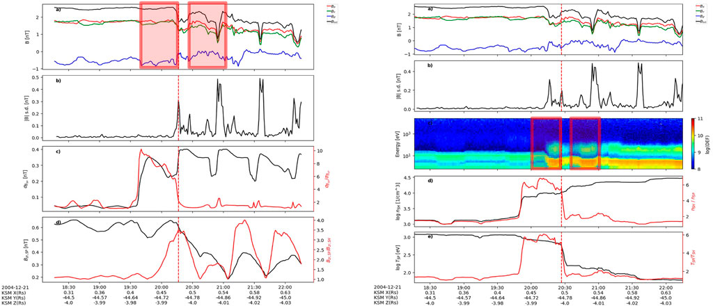
FIGURE 6. (A) of both subplots show the magnetic field components and magnitude. (B) of both subplots show the standard deviation of the magnetic field magnitude. thresh-mag (left): Threshold method to detect boundary crossings using four magnetic field parameters: B standard deviation in SH [(C) black line], the ratio of B standard deviation between SH and SP [(C) red line], North-south/radial component of B in SP [(D) black line], and the ratio of Bz or Br between SP and SH [(D) red line]. thresh-caps (right): Threshold method to detect boundary crossings using four density and temperature parameters: log electron density in SH [(D) black line], the ratio of density between SH and SP [(D) red line], log temperature in SP [(E) black line], and the ratio of temperature between SP and SH [(E) red line]. For both methods, threshold values were acquired using Bayesian optimisation.

A positive detection occurs when a fixed threshold is exceeded in all the parameters. To find the most suitable parameter thresholds which maximise the number of true crossings being discovered (recall) whilst also maximising the number of true positives (precision), Bayesian optimisation was used to ‘train’ the threshold model to maximise the F1 score over all the training data (2004–2011). The F1 score is defined as

$F_1=\frac{2}{1/P+1/R}.(4)$

It is a harmonic mean of precision and recall, meaning the F1 score is more sensitive to smaller values of precision (P) or recall (R). Precision, which measures how accurate are the predictions, is given by

$\text{P}=\frac{TP}{TP+FP},(5)$

i.e., the fraction of positive predictions (TP + FP) that is actually true (TP). Recall, which measures how good the model finds all the positives, is given by

$\text{R}=\frac{TP}{TP+FN},(6)$

i.e., the fraction of positive instances (TP + FN) that is correctly predicted (TP). Here, TP, FP, and TN represent true positive, false positive and true negative. The Bayesian optimisation routine was implemented using the Botorch package in Python Balandat et al. (2020). The outline of the procedure is as follows:

1. The initial sampling set is the initial guess of parameter values to be optimised. For this study, the thresholds of the magnetic field and electron parameters were the parameters to guess.

2. Black-box problem evaluation is performed by looping through the dataset using this set of parameter thresholds and the desired target metric is evaluated.

3. A Gaussian process (GP) would predict what the target metric would be for other input parameter thresholds.

4. Evaluate the acquisition function to decide what input parameters to test next. This process uses a Monte-Carlo sampler. For example, to minimise some metric, the lower confidence bound acquisition function a(x) = f(x) − κσ(x) can be used where κ is a hyperparameter of the optimisation problem, f(x) is the mean of the GP, σ is the standard deviation at input x.

5. The next point to evaluate the target will be at arg min_x (a(x)). i.e., the parameter thresholds which would decrease (or increase) the target function (depending on the goal of the optimisation).

6. Iterate until convergence, that is when the target function no longer improves for a consecutive number of iterations. Typically, 100 loops of optimisation were found to work well.

The classification between BS and MP is further determined from the windowed statistics of each interval. A big drawback of using the threshold method with magnetic field data was the existence of a significant number of MP crossings with low magnetic shear (Masters et al., 2012) meaning that there may not be a sufficient ratio in B_zr,SP/B_zr,SH. Despite the use of four criteria in the ‘thresh-mag’ method, the precision remains low (i.e., large number of false positives).

2.3.2 ResNet18: Convolutional neural network

The convolutional neural network (CNN) method for boundary classification was motivated by how the existing catalogue of crossings was created. The data were manually surveyed by human eyes looking for characteristic features of BS and MP as described in Section 2.2.1. This bodes well for attempting automation with computer vision models. The model architecture consisted of two parts: a feature learning network and a classification network. The ResNet18 was used for the first part with 18 convolutional layers, followed by a fully connected neural network with two layers for the second part. More details of the model architecture can be found in Section 1.3 of the Supplementary Material. The number of training epochs was set to 30 but generally it was found that training curves plateaued around 10 epochs.

Figure 7 shows an input image of the CAPS electron energy spectrogram passed through the CNN giving output ‘crossing’ or ‘notCrossing’. Similar to how the four parameters (or features) for the threshold method were created based on input MAG or CAPS time-series, a CNN automatically finds discriminative features from the input image by training with the ground truth labels for each plot.

FIGURE 7

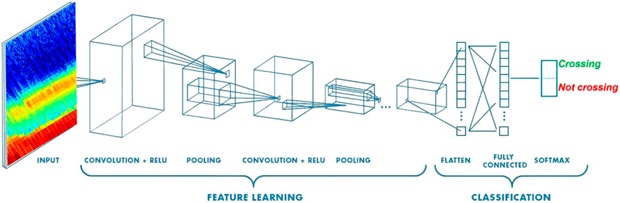
FIGURE 7. Diagram showing how an input image of CAPS ELS energy spectrogram is passed through a CNN model and is classified as being a ‘crossing’ or ‘notCrossing’.

Both the threshold and CNN models would accomplish the task of automation in principle because they were designed to look for patterns commonly found in BS and MP crossings. A natural question to ask is: why did the algorithm produce a particular output? Can the model outputs be explained?

2.3.3 Model explainability

For the threshold method, it was obvious why a prediction was made based on the values of the four parameter thresholds which discriminate a crossing from a non-crossing.

For CNN, the Grad-CAM technique (Selvaraju et al., 2020) was used to visually explain the neural network’s output. This technique overlays a heatmap on top of an image of interest to indicate pixel regions which are most discriminative for the output class. The values which make up the heatmap are a linear combination of the activation function value in each channel in the last layer, weighted by the gradient of the loss with respect to the parameters in the last convolutional layer.

Figure 8 shows an example of Grad-CAM applied to MAG and CAPS plots using the implementation by Gildenblat. (2021). The red regions (or equivalently regions of concentrated contour lines) highlight the most important parts of the image considered by the final layer of the CNN. Experiments were performed using Grad-CAM on a series of BS CAPS plots striding forward in time in steps of 6 min. It was observed that for the different input images, the red region tracked well where the discontinuity was, which mimicked what human eyes would focus on for making predictions. This was a good indication that the neural network was focusing on the right features in the image to generate the correct classification.

FIGURE 8

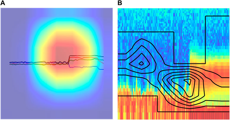
FIGURE 8. Grad-CAM applied to cnn-mag (A) and cnn-caps (B) images for the interval 2012-03-21 23:30:00 to 2012-03-22 01:30:00. The heatmap shows regions which are most discriminative for the output class. For the MAG image (A), the red regions highlight the most important pixels for the target class. For the CAPS image (B), the regions with more contour lines indicate the most important pixels for the target class. Both models highlight the region with discontinuity as most important, which is what our eyes would focus on for deciding between crossing or not. The y-scale of the MAG image ranges from -10 nT to 10 nT. The y-scale of the CAPS image ranges from 0.6 eV to 28.25 keV on a logarithmic scale consisting of the 63 energy bins of the CAPS ELS instrument. Both images show the same 2-h interval of Cassini data.

2.3.4 Error analysis

After training and evaluating the models, error analysis was performed to understand where the algorithms were making mistakes. One of the major problems found was the lack of label consistency in the existing crossing list. An example was found in a high latitude MP crossing in the interval 2009-02-10 17:13:00 to 2009-02-10 19:13:00 (Supplementary Figure S2); the timestamp for this event from independently derived, expert identified catalogues by Pilkington et al. (2015) and Jackman et al. (2019) were 1 hour apart. The Bayesian optimised MAG and CAPS threshold methods predicted a crossing at around 18:00 which was between the two human labels, whilst the CNN model also predicted a crossing for this 2-h interval. Label inconsistency is particularly detrimental to supervised learning algorithms because its goal is to learn a mapping between the input MAG or CAPS data (X) and output label (y). A noisy set of labels would lead to a noisy mapping, thus low accuracy. Attempts were made to clean up the labels by using a set of clearer labelling instructions and also exclude samples which were ambiguous from the training data as these could deteriorate the performance of the final model.

2.3.5 Other potential automation techniques

Other techniques were explored using mathematical models of the MP boundary to design a series of physical checks to determine if the selected candidates were genuine BS, MP or neither.

Assuming that MP crossings were oriented similar to those predicted by an MP model [e.g., Kanani et al. (2010)], another method that was thought to be a good physical check was the use of minimum variance analysis (MVA) to determine the orientation of Saturn’s MP surface at the time of each crossing and compare it with the model normal. The angular difference between them could be used to double check the validity of the proposed crossing based on our physical knowledge of the MP boundary. In this physical check, for every candidate center crossing time, a series of window sizes (6, 10, 14, 20, 30, 40, 60) in minutes were used to calculate the MVA normal. An estimate of the smallest angle between the MVA normal and the model normal was found, and similarly between the MVA normal and the tangential discontinuity (TD) normal could also be made (Sonnerup and Scheible, 1998). Crossings could be discarded if they exceeded a certain threshold of this angular difference. However, the orientation of the normal was highly dependent on the identification of intervals corresponding to the magnetopause current layer (MPCL) where the field direction persistently changes. The MPCL interval has to be done by eye currently and thus is not yet possible to automate. Furthermore, there was a significant number of cases where, even by eye, the identification of the MPCL interval was ambiguous, especially in cases where there was a low magnetic shear between the magnetospheric and magnetosheath magnetic fields. This physical check was discarded in the end as it did not offer any boost in the performance compared with more simple checks (such as using the magnetic field magnitude alone), whilst also requiring more computational cost.

Another technique to check whether the selected candidates were true MP crossings or not was to fit a magnetic pressure model using the existing list of magnetopause crossings assuming a dipole approximation. Using the functional form of the magnetopause given by (Pilkington et al., 2015) and applying pressure balance at the MP boundary, a value of β could be estimated for the candidate which can be compared with the distribution of β values found for genuine MP crossings. It was suspected that, due to the pressure balance nature of the MP boundary, events which were not genuine should have a predicted β which would be in the tail of the distribution for genuine MP crossings. However, the opposite was found to be true; many events which were not genuine crossings also had typical β values, within 1 standard deviation of the mean log(β) distribution from the Pilkington et al. (2015) MP crossing list. Thus, this physical check was not used.

2.4 Deployment

The rapid inference time of the CNN model makes it a suitable candidate for usage onboard the spacecraft. The ResNet18 model has a size of 42.8 MB which is small compared to the onboard storage of 2 Gb (gigabits) in the form of dynamic random access memory (DRAM) on Cassini. However, the actual inference times may differ depending on the availability of hardware acceleration onboard the spacecraft. Compression techniques such as pruning and quantization of trained models could also be leveraged to significantly decrease the overall resource requirements for deploying such networks on mobile devices with limited resources (Berthelier et al., 2019). Furthermore, as the model inputs are JPEG or PNG images of the data plots, it requires minimal processing, unlike other detection methods. After deployment, the performance of the system would be continuously monitored by the human-in-the-loop to ensure data drift or concept drift are not affecting the system. Data drift occurs when the input distribution is changed relative to the training data. This could be drastic changes to the spacecraft orbit to monitor a different region of space which changes the input data distribution. In this case, the model should be retrained with the inclusion of the new data and corresponding labels. Concept drift occurs when the mapping between input and output changes. This could be due to changes in the sensitivity of the instruments during the space mission, such that the same phenomena now correspond to different instrumental measurements. Therefore, human-in-the-loop is still crucial to ensure the proper long-term functioning of the automated system.

3 Results and discussion

The results of this study are reported using precision, recall and F1 scores for corresponding models investigated. These metrics are summarised in Table 1 for the threshold and CNN models. The performance scores are relative to the ground truth provided by Jackman et al. (2019) boundary crossing list. However, these performance metrics may differ upon further refinement of the crossing list. At the time of the current study, it was found that the cnn-caps outperformed all other methods based on the recall (88.7%) and F1-score (72.5%) metrics.

TABLE 1

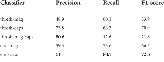
TABLE 1. Performance comparison for different models. Precision (P) is the % of predictions which are correct. Recall (R) is the % of ground truth which are predicted correctly. F1-score is the harmonic mean of precision and recall (Eq. 4). Note that the tolerance for correct classification for ‘thresh-’ classifiers was set at ± 60 min from the ground truth crossing times. The bold values represent the model which achieved the best score for that specific metric.

3.1 Model comparison: Performance

The performance of the two methods was expected to be different due to the difference in the locality with which features were generated. The threshold method extracted features using two 30-min windows with a fixed gap of 8 min whilst the CNN method extracted features from a 2-h window.

Considering the threshold method, when optimising for the F1-score (Eq. 4) on a global scale (i.e., evaluating the performance using all crossings from all years), the thresh-caps method generally produced consistently better performance metrics across the years 2004–2012 than thresh-mag as seen in Figure 9. Further experimentation was done such as ensembling the MAG and CAPS threshold features together. This had the expected result of massively improved precision for some years compared to the magnetic-field-only method, exceeding the recall in all years (Figure 9C). The amount of improvement varied across the different years of orbits, in some cases doubling from 30% to 60% such as in the year 2009, whilst other years the improvement was more modest from 60% to 62% such as in the year 2005. However, the recall naturally dropped significantly due to more criteria to satisfy to make a positive detection, reducing the number of positive detections. Another problem associated with this method was the fact that the thresholds were picking up both BS and MP. This was not unexpected as BS crossings typically have even larger values in the parameters considered thus more easily satisfying the thresholds set for MP crossings. There was no single way to separate the two types of crossings using thresholds alone due to the large variations of both types of crossings. There were attempts to further refine the classifications using the magnetic field magnitude as it was one of the biggest differentiating factors between BS and MP crossings. However, the issue was still the sheer number of false positive detections that were retrieved using the threshold method. This lead to poor precision when considering the retrieval of a single class of crossing.

FIGURE 9

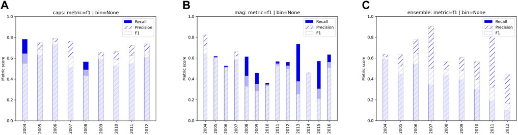
FIGURE 9. Comparison of performance for three threshold models. (A) thresh-caps. (B) thresh-mag. (C) thresh-ensemble. In the calculation of these metrics, BS crossings were included in the ground truth dataset. All models were optimised based on the F1 score.

An experiment was conducted to optimise the F1-score for different location sectors to investigate the dependence of the threshold method on the crossing location. The sectors were defined based on local time (DAWN 3 h–9 h, DAY 9 h–15 h, DUSK 15 h–21 h) and absolute latitude (LOW 0°–30°, MID 30°–60°, and HIGH 60°–90°). The majority (92%) of the true BS and MP crossings between 2004–2012 were in the LOW latitude bins (across all local times), with a small percentage (8%) in bins of DAYMID, DUSKMID and DUSKHI. For the years 2013–2016, 69% of true crossings were in the LOW latitude bins, and the remaining 31% were distributed amongst the DAWNMID, DAYMID, and DUSKMID bins.

By performing Bayesian optimisation for each bin, a set of thresholds was obtained for each bin (Figure 10). It was found that there was large variability in performance across different years for each bin, which indicated that a threshold which does well for 1 year may not be applicable for another. This is likely due to changing conditions from the Sun, changing spacecraft radial distance and other plasma processes which could change the nature of the boundary crossings. For dusk crossings, the magnetodisc plasma sheet could expand more due to solar wind direction being the same as corotation flow, leading to less turbulent conditions. Therefore, the ‘typical’ features of an MP transition may not be as common. There could also be lots of genuine partial crossings which are being picked up but that may not be in the ground truth (i.e., large number of false positives), lowering the precision (Eq. 5). Bins with fewer crossings were found to perform better likely because the thresholds were over-fitted to just capture those few crossings. Bins with more crossings (e.g., in the LOW latitude bin) have lower performance as the single set of optimised thresholds fails to capture the variety of crossings observed at low latitudes.

FIGURE 10

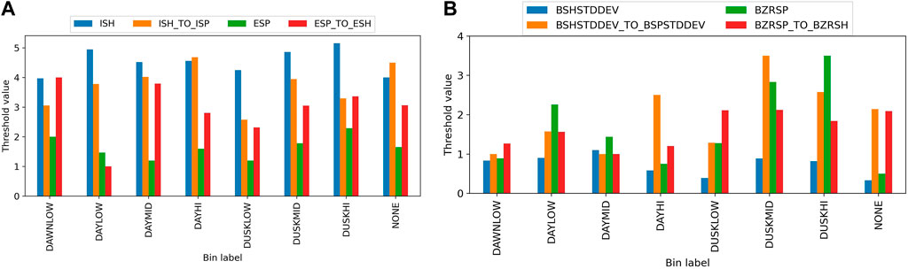
FIGURE 10. The threshold values for MAG data (A) and CAPS data (B) were found from the Bayesian optimisation routine for each local time and latitude bin containing mag and caps data. The final bin label ‘None’ indicates the thresholds found from the global optimisation with all crossings used.

When considering magnetic-field-only detections, the worst performing local time sector was dusk, likely due to missed partial crossings and or more false positives. It may also be that the magnetic fields are more dynamic over timescales similar to an MP crossing, leading to less well-defined transitions. The lack of difference between either side of the transition is particularly detrimental to the threshold method given that it uses the ratios of quantities from two windows of data. The year 2007 was particularly problematic when trying to define consistent crossing times. However, due to a large number of detections, it was unfeasible to perform an error analysis of each positive detection as was done for the CNN method.

Considering the CNN method, given that the cnn-caps model outperformed other models in the binary classification task, a multiclass cnn-caps model was then chosen to be trained in order to classify 2-h intervals of electron spectrogram data as ‘BS’, ‘MP’ or ‘notCrossing’. The model performance on the training and validation dataset was tested with 10-fold cross-validation and was found to be consistent across all 10-folds for a given model architecture. This implies that the model was not too sensitive to the choice of samples in the training and validation sets. The results are summarised in Supplementary Table S1 in the Supplementary Material. The model variance, defined as the difference between training and validation error, could be used to indicate signs of over-fitting. The error is obtained from the mean cross entropy loss (Eq. 2) calculated during model training, ranging from 0 to 1, with 0 being perfect classification. From the cross-validation experiment, the average model variance was low at around 0.10 ± 0.04. This result implies that the model was not suffering from over-fitting to the training data. The model with the lowest validation error from cross-validation was used to evaluate the performance on the test dataset. To estimate uncertainty in the test performance metrics, 1,000 bootstrap samples of the test dataset with replacements were used (Kohavi, 1995). The histograms of precision, recall, and F1 for each class are shown in Supplementary Figure S5 in the Supplementary Material from which uncertainties were estimated using the standard deviation (given the similarity to Gaussian distributions). Through error analysis of 196 misclassified samples, it was revealed that 48.5% were MP crossings, 26.5% were BS, 12.2% occurred in the magnetosheath, 11.7% occurred in the magnetosphere, 1.0% occurred in the solar wind. There were 15 samples which had missing CAPS data within the defined intervals whilst ground truth labels were provided using MAG data. These were removed from the test dataset which reduced the number of test samples from 3,032 to 3,017. Table 2 shows the performance of the multiclass cnn-caps model when the test dataset was corrected to include previously missed BS and MP crossings. The results indicate that the cnn-caps model was able to detect ‘notCrossing’ class with high precision and recall, BS crossings with very high precision but slightly lower recall, and MP crossings with reasonable precision and recall. The resulting F1 scores (Eq. 4) for the classes of interest were 92.1% ± 1.4% and 84.7% ± 1.9% for BS and MP crossings respectively.

TABLE 2

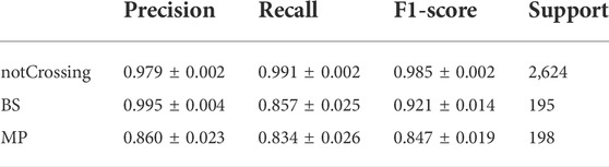
TABLE 2. Performance metrics of the cnn-caps classifier after correction of the labels in the previously misclassified samples. The support columns indicate the number of samples for each class. The uncertainty in each metric was estimated using the standard deviation of 1,000 bootstrap samples of the corrected test dataset evaluated using the same model.

The threshold method is intuitive for event detection but it lacks the flexibility due to fixed thresholds to capture events especially when the variety of crossings is large, even within the same type of boundary, such as MP crossings. On the other hand, neural network models have enough parameters to offer more flexibility to find a wider range of events without over-fitting.

One of the major advantages of neural network models is that once the algorithm is trained, the inference speed is extremely fast. For the sake of comparison, for the same 2-h interval, the trained cnn-caps model performs inference on the order of 10 ms on a laptop equipped with NVIDIA GeForce GTX 1650, whilst the thresh-mag model takes the order of 1s to predict whether there is a crossing, which is 100 times slower than the cnn-caps method. Therefore, in an onboard data selection scenario, it is advantageous to leverage the speed of neural networks in order to perform the first level of data selection before fine-tuning with other techniques such as manual inspection.

3.2 A new BS and MP crossings list for saturn

The benefit of having an automated system is that it can be used to scan through all the data without extra human effort. This allows the discovery of new events which could have been missed despite being obvious. For example, the interval between 2005-07-28 14:00:00 and 2005-07-28 16:00:00 had a data gap in the MAG data but was easily detected from CAPS data using cnn-caps.

To this end, a new comprehensive list of BS and MP crossings from Cassini have been identified with the help of the models developed in this study, building on the lists found by Jackman et al. (2019) and Pilkington et al. (2015). All new crossings added were ensured to be consistent with previously identified crossing directions. For example, an inbound MP crossing must be followed by an outbound MP crossing.

The new list contains 1349 BS crossings and 2539 MP crossings, representing an 8% and 20% increase compared to the original list with 1249 BS and 2124 MP, respectively.

The breakdown of the number of crossings across different years of the mission from Saturn-Orbit-Insertion in July 2004 to when the CAPS instrument was switched off in June 2012 is shown in Table 3.

TABLE 3

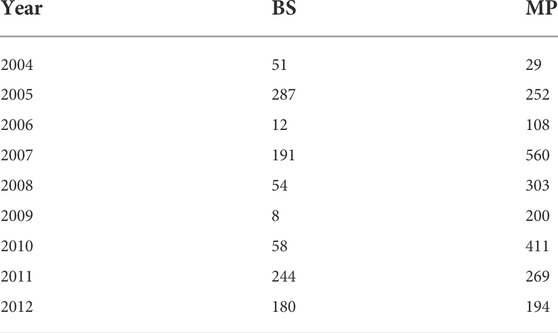
TABLE 3. Breakdown of the number of bow shock (BS) and magnetopause (MP) crossings in the new list of boundary crossings between years 2004–2012.

Interesting case studies could be discovered by inspecting through the positive detections. For example, Figure 11 shows a ‘crossing’ event recorded between 2012-05-14 05:00:00 and 2012-05-14 07:00:00 picked up by the CNN method that was not previously identified in any crossing list appeared to be a candidate K-H vortex encounter. This event was situated on the dusk flank near the equator. There was periodic sign change in B_y and striking electron and ion energization signature similar to that discussed in Masters et al. (2010).

FIGURE 11

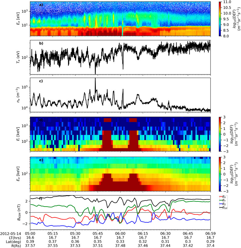
FIGURE 11. A 2-h interval encompassing a potential K-H vortex encounter. The panels are as follows: (A) Electron energy-time spectrogram of differential energy flux (DEF) from CAPS/ELS anode 5. (B,C) Electron temperature and number density derived from ELS anode 5. (D,E) Energy-time spectrogram of ion and electron intensity from LEMMS. (F) The magnitude and KSM components of the magnetic field. Spacecraft trajectory information is shown below the x-axis.

In a future study, there is potential to turn the CNN classifier into both a region and a boundary classifier, by altering the training labels with six classes: SW, BS, SH, MP, SP and Other. The ‘Other’ class can be thought of as an ‘uncertainty’ class which should be looked at by the ‘human-in-the-loop’, as well as the precise crossing times for each BS and MP crossing classified. One could also explore the possibilities of fine-tuning the classifier for boundary detection at other planets. Since BS and MP crossings at different planets share common magnetic field and plasma signatures (e.g., as described in Section 2.2.1), at least visually, the weights of the ResNet18 portion of the CNN classifier could be kept fixed, whilst the weights in the classifier ‘head’ could be fine-tuned by training on a consistently labelled crossings dataset for the planet of interest. This greatly reduces the number of learned parameters in the neural network, thus, significantly reduces the training time and the size of the dataset required.

ML algorithms can help automate a manual process. However, when the algorithm’s ability is not yet fully reliable, the degree of automation falls short of fully automatic detection. Nevertheless, having partial automation and keeping the human-in-the-loop can still hugely accelerate the process of crossing identification.

4 Conclusion

The key points of this study can be summarised as follows:

1. Two methods for automating the detection of the bow shock and magnetopause crossings in Cassini data were implemented and compared: Threshold-based detection and convolutional neural network (CNN) classifier. Based on 2012 test data and the latest BS and MP catalogue at Saturn, the CNN approach outperformed the threshold approach when considering CAPS data. Cassini MAG and CAPS/ELS datasets were used as the data source. However, the methods demonstrated would also be applicable to other spacecraft missions with magnetic field and plasma data.

2. It is possible to automate the detection of BS and MP crossings using magnetic field data and/or electron energy spectrograms as demonstrated with Cassini data at Saturn. However, it was found that for both methods the electron-only data model outperformed the magnetic-field-only model, for the period where both instruments did not have missing data. Combining both datasets lead to higher precision but lower recall as expected. For discovering more crossings, ‘thresh-mag’ could be used with higher thresholds to ensure a higher probability of correct identification of typical BS or MP crossing events. The ability to select specific types of events which exceed definitive thresholds is an advantage of the threshold method, which is not possible with the CNN model.

3. The ResNet18 CNN model is small (42.8 MB) and once trained has fast inference times (of order 10 ms) which makes it suitable for on-board spacecraft data selection or performing large-scale boundary surveys in post-mission data analysis.

Data availability statement

The original contributions presented in the study are included in the article/Supplementary Material, further inquiries can be directed to the corresponding author.

Author contributions

IC wrote the code, analysed the results and wrote the main manuscript. NA and AS directed the various experiments. All authors reviewed the manuscript.

Funding

IC was supported by a UK STFC studentship hosted by the UCL Centre for Doctoral Training in Data Intensive Science (Grant Number ST/P006736/1). NA was supported by UK STFC Consolidated Grant Number ST/S000240/1 (UCL/MSSL-Physics and Astronomy Solar System). AS was supported by NERC grants NE/P017150/1 and NE/V002724/1. For the purpose of open access, the author has applied a Creative Commons Attribution (CC BY) licence to any Author Accepted Manuscript version arising.

Acknowledgments

The authors wish to thank Caitriona Jackman for thoughtful discussions and useful comments about this work. The Cassini MAG and ELS data are available from the Planetary Data System (http://pds.nasa.gov/).

Conflict of interest

The authors declare that the research was conducted in the absence of any commercial or financial relationships that could be construed as a potential conflict of interest.

Publisher’s note

All claims expressed in this article are solely those of the authors and do not necessarily represent those of their affiliated organizations, or those of the publisher, the editors and the reviewers. Any product that may be evaluated in this article, or claim that may be made by its manufacturer, is not guaranteed or endorsed by the publisher.

Supplementary material

The Supplementary Material for this article can be found online at: https://www.frontiersin.org/articles/10.3389/fspas.2022.1016453/full#supplementary-material

Footnotes

¹Timestamp notation: YYYY-MM-DD HH:MM:SS.

References

Achilleos, N., Bertucci, C., Russell, C. T., Hospodarsky, G. B., Rymer, A. M., Arridge, C. S., et al. (2006). Orientation, location, and velocity of Saturn’s bow shock: Initial results from the Cassini spacecraft. J. Geophys. Res. 111, A03201–A03218. doi:10.1029/2005JA011297

CrossRef Full Text | Google Scholar

Argall, M. R., Small, C. R., Piatt, S., Breen, L., Petrik, M., Kokkonen, K., et al. (2020). MMS SITL ground loop: Automating the burst data selection process. Front. Astron. Space Sci. 7, 54. doi:10.3389/fspas.2020.00054

PubMed Abstract | CrossRef Full Text | Google Scholar

Bakrania, M. R., Rae, I. J., Walsh, A. P., Verscharen, D., and Smith, A. W. (2020). Using dimensionality reduction and clustering techniques to classify space plasma regimes. arXiv 7, 1–12. doi:10.3389/fspas.2020.593516

CrossRef Full Text | Google Scholar

Balandat, M., Karrer, B., Jiang, D. R., Daulton, S., Letham, B., Wilson, A. G., et al. (2020). BoTorch: A framework for efficient monte-carlo bayesian optimization. In Advances in Neural Information Processing Systems, 33.

Google Scholar

Berthelier, A., Phutane, P., Duffner, S., Garcia, C., Blanc, C., and Chateau, T. (2019). Deep model compression for mobile devices : A survey

Google Scholar

Breuillard, H., Dupuis, R., Retino, A., Contel, O. L., Amaya, J., and Lapenta, G. (2020). Automatic classification of plasma regions in near-Earth space with supervised machine learning: Application to magnetospheric multi scale 2016–2019 observations. Front. Astron. Space Sci. 7. doi:10.3389/fspas.2020.00055

CrossRef Full Text | Google Scholar

Case, N. A., and Wild, J. A. (2013). The location of the Earth’s magnetopause: A comparison of modeled position and in situ cluster data. J. Geophys. Res. Space Phys. 118, 6127–6135. doi:10.1002/jgra.50572

CrossRef Full Text | Google Scholar

Cheng, I., Achilleos, N., Masters, A., Lewis, G., Kane, M., and Guio, P. (2021). Electron bulk heating at saturn's magnetopause. JGR. Space Phys. 126. doi:10.1029/2020ja028800

CrossRef Full Text | Google Scholar

da Silva, D., Barrie, A., Shuster, J., Schiff, C., Attie, R., Gershman, D. J., et al. (2020). Automatic region identification over the mms orbit by partitioning n-t space. doi:10.48550/ARXIV.2003.08822

CrossRef Full Text | Google Scholar

Daigavane, A., Wagstaff, K. L., Doran, G., Cochrane, C. J., Jackman, C. M., and Rymer, A. (2022). Unsupervised detection of saturn magnetic field boundary crossings from plasma spectrometer data. Comput. Geosciences 161, 105040. doi:10.1016/j.cageo.2022.105040

CrossRef Full Text | Google Scholar

Dougherty, M. K., Kellock, S., Southwood, D. J., Balogh, A., Smith, E. J., Tsurutani, B. T., et al. (2004). The Cassini magnetic field investigation. Space Sci. Rev. 114, 331–383. doi:10.1007/s11214-004-1432-2

CrossRef Full Text | Google Scholar

Gildenblat (2021). Pytorch library for cam methods. Available at: https://github.com/jacobgil/pytorch-grad-cam.

Google Scholar

Gilet, N., Leon, E. D., Gallé, R., Vallières, X., Rauch, J.-L., Jegou, K., et al. (2021). Automatic detection of the thermal electron density from the WHISPER experiment onboard CLUSTER-II mission with neural networks. JGR. Space Phys. 126. doi:10.1029/2020ja028901

CrossRef Full Text | Google Scholar

Goodfellow, I., Bengio, Y., and Courville, A. (2016). Deep learning. MIT Press. Available at: http://www.deeplearningbook.org.

Google Scholar

He, K., Zhang, X., Ren, S., and Sun, J. (2016). “Deep residual learning for image recognition,” in Proceedings of the IEEE computer society conference on computer vision and pattern recognition, 2016, 770–778. doi:10.1109/CVPR.2016.90

CrossRef Full Text | Google Scholar

Hinton, G. E., and Salakhutdinov, R. R. (2006). Reducing the dimensionality of data with neural networks. Science 313, 504–507. doi:10.1126/science.1127647

PubMed Abstract | CrossRef Full Text | Google Scholar

Jackman, C., Thomsen, M., and Dougherty, M. (2019). Survey of Saturn’s magnetopause and bow shock positions over the entire cassini mission: Boundary statistical properties, and exploration of associated upstream conditions. JGR. Space Phys. 124, 8865–8883. doi:10.1029/2019ja026628

CrossRef Full Text | Google Scholar

Joy, S. P., Kivelson, M. G., Walker, R. J., Khurana, K. K., Russell, C. T., and Paterson, W. R. (2006). Mirror mode structures in the Jovian magnetosheath. J. Geophys. Res. 111, A12212–A12214. doi:10.1029/2006JA011985

CrossRef Full Text | Google Scholar

Kanani, S. J., Arridge, C. S., Jones, G. H., Fazakerley, A. N., McAndrews, H. J., Sergis, N., et al. (2010). A new form of Saturn’s magnetopause using a dynamic pressure balance model, based on in situ, multi-instrument Cassini measurements. J. Geophys. Res. 115, 1–11. doi:10.1029/2009JA014262

CrossRef Full Text | Google Scholar

Kim, K.-C., and Lee, D.-Y. (2014). Magnetopause structure favorable for radiation belt electron loss. J. Geophys. Res. Space Phys. 119, 5495–5508. doi:10.1002/2014JA019880

CrossRef Full Text | Google Scholar

Kingma, D. P., and Ba, J. L. (2015). Adam: A method for stochastic optimization. In 3rd International Conference on Learning Representations, ICLR 2015 - Conference Track Proceedings, 1–15.

Google Scholar

Kohavi, R. (1995). A study of cross-validation and bootstrap for accuracy estimation and model selection. In Proc. 14th Int. Jt. Conf. Artif. Intell. - 2IJCAI’95. San Francisco, CA, USA: Morgan Kaufmann Publishers Inc., 1137–1143.

Google Scholar

Le, G., and Russell, C. T. (1994). The thickness and structure of high beta magnetopause current layer. Geophys. Res. Lett. 21, 2451–2454. doi:10.1029/94GL02292

CrossRef Full Text | Google Scholar

LeCun, Y., Haffner, P., Bottou, L., and Bengio, Y. (1999). Object Recognition with Gradient-Based Learning, 319–345. doi:10.1007/3-540-46805-6_19

CrossRef Full Text | Google Scholar

Masters, A., Achilleos, N., Cutler, J., Coates, A., Dougherty, M., and Jones, G. (2012). Surface waves on Saturn’s magnetopause. Planet. Space Sci. 65, 109–121. doi:10.1016/j.pss.2012.02.007

CrossRef Full Text | Google Scholar

Masters, A., Achilleos, N., Kivelson, M. G., Sergis, N., Dougherty, M. K., Thomsen, M. F., et al. (2010). Cassini observations of a Kelvin-Helmholtz vortex in Saturn’s outer magnetosphere. J. Geophys. Res. 115, 1–13. doi:10.1029/2010JA015351

CrossRef Full Text | Google Scholar

Masters, A., Mitchell, D. G., Coates, A. J., and Dougherty, M. K. (2011). Saturn’s low-latitude boundary layer: 1. Properties and variability. J. Geophys. Res. 116, 1–13. doi:10.1029/2010JA016421

CrossRef Full Text | Google Scholar

Masters, A., Phan, T. D., Badman, S. V., Hasegawa, H., Fujimoto, M., Russell, C. T., et al. (2014). The plasma depletion layer in Saturn’s magnetosheath. J. Geophys. Res. Space Phys. 119, 121–130. doi:10.1002/2013JA019516

CrossRef Full Text | Google Scholar

McAndrews, H. J., Owen, C. J., Thomsen, M. F., Lavraud, B., Coates, A. J., Dougherty, M. K., et al. (2008). Evidence for reconnection at Saturn’s magnetopause. J. Geophys. Res. 113. doi:10.1029/2007JA012581

CrossRef Full Text | Google Scholar

NASA Jet Propulsion Laboratory (2017). Cassini huygens by the numbers. Retrieved from Available at: https://solarsystem.nasa.gov/resources/17761/cassini-huygens-by-the-numbers/.

Google Scholar

Nguyen, G., Aunai, N., de Welle, B. M., Jeandet, A., and Fontaine, D. (2019). Automatic detection of the earth bow shock and magnetopause from in-situ data with machine learning. doi:10.5194/angeo-2019-149

CrossRef Full Text | Google Scholar

Olshevsky, V., Khotyaintsev, Y. V., Lalti, A., Divin, A., Delzanno, G. L., Anderzén, S., et al. (2021). Automated classification of plasma regions using 3d particle energy distributions. JGR. Space Phys. 126. doi:10.1029/2021ja029620

CrossRef Full Text | Google Scholar

Paszke, A., Gross, S., Massa, F., Lerer, A., Bradbury, J., Chanan, G., et al. (2019). “Pytorch: An imperative style, high-performance deep learning library,” in Advances in neural information processing systems 32. Editors H. Wallach, H. Larochelle, A. Beygelzimer, F. d'Alché-Buc, E. Fox, and R. Garnett (Atlanta, GA: Curran Associates, Inc.).

Google Scholar

Phan, T. D., Drake, J. F., Shay, M. A., Gosling, J. T., Paschmann, G., Eastwood, J. P., et al. (2014). Ion bulk heating in magnetic reconnection exhausts at Earth’s magnetopause: Dependence on the inflow Alfvén speed and magnetic shear angle. Geophys. Res. Lett. 41, 7002–7010. doi:10.1002/2014GL061547

CrossRef Full Text | Google Scholar

Phan, T. D., Shay, M. A., Gosling, J. T., Fujimoto, M., Drake, J. F., Paschmann, G., et al. (2013). Electron bulk heating in magnetic reconnection at Earth ’ s magnetopause : Dependence on the in fl ow Alfvén speed and magnetic shear. Geophys. Res. Lett. 40, 4475–4480. doi:10.1002/grl.50917

CrossRef Full Text | Google Scholar

Pilkington, N. M., Achilleos, N., Arridge, C. S., Guio, P., Masters, A., Ray, L. C., et al. (2015). Asymmetries observed in Saturn’s magnetopause geometry. Geophys. Res. Lett. 42, 6890–6898. doi:10.1002/2015GL065477

PubMed Abstract | CrossRef Full Text | Google Scholar

Sak, H., Senior, A., and Beaufays, F. (2014). Long short-term memory based recurrent neural network architectures for large vocabulary speech recognition

Google Scholar

Selvaraju, R. R., Cogswell, M., Das, A., Vedantam, R., Parikh, D., and Batra, D. (2020). Grad-CAM: Visual explanations from deep networks via gradient-based localization. Int. J. Comput. Vis. 128, 336–359. doi:10.1007/s11263-019-01228-7

CrossRef Full Text | Google Scholar

Sonnerup, B., and Scheible, M. (1998). Minimum and maximum variance analysis. Analysis methods Spacecr. data 001 (8), 185–220.

Google Scholar

Sulaiman, A. H., Masters, A., and Dougherty, M. K. (2016). Characterization of Saturn’s bow shock: Magnetic field observations of quasi-perpendicular shocks. J. Geophys. Res. Space Phys. 121, 4425–4434. doi:10.1002/2016JA022449

CrossRef Full Text | Google Scholar

Went, D. R., Hospodarsky, G. B., Masters, A., Hansen, K. C., and Dougherty, M. K. (2011). A new semiempirical model of Saturn’s bow shock based on propagated solar wind parameters. J. Geophys. Res. 116, 1–9. doi:10.1029/2010JA016349

CrossRef Full Text | Google Scholar

Yeakel, K. L., Vandegriff, J. D., Garton, T. M., Jackman, C. M., Clark, G., Vines, S. K., et al. (2022). Classification of cassini’s orbit regions as magnetosphere, magnetosheath, and solar wind via machine learning. Front. Astron. Space Sci. 9. doi:10.3389/fspas.2022.875985

CrossRef Full Text | Google Scholar

Young, D. T., Berthelier, J. J., Blanc, M., Burch, J. L., Bolton, S., Coates, A. J., et al. (2005). Composition and dynamics of plasma in Saturn’s magnetosphere. Science 307, 1262–1266. doi:10.1126/science.1106151

PubMed Abstract | CrossRef Full Text | Google Scholar

Young, D. T., Berthelier, J. J., Blanc, M., Burch, J. L., Coates, A. J., Goldstein, R., et al. (2004). Cassini plasma spectrometer investigation. Space Sci. Rev. 114, 1–112. doi:10.1007/s11214-004-1406-4

CrossRef Full Text | Google Scholar