Full-wave modeling of EMIC wave packets: ducted propagation and reflected waves

1 Introduction

The electromagnetic ion cyclotron (EMIC) wave is a type of electromagnetic emission that is generated by unstable anisotropic ion distributions (Cornwall, 1965; Anderson et al., 1996; Min et al., 2015) and interacts with relativistic and ultrarelativistic electrons in the Earth’s radiation belts (Horne and Thorne, 1998; Summers et al., 1998; Li and Hudson, 2019; Baker, 2021). The wave frequencies are typically extremely low, ranging from f = 0.1 Hz to f = 5.0 Hz (Saito, 1969). More precisely, the upper-frequency limit is determined by the proton cyclotron frequency (f_cp) in the source, which is much smaller than the electron gyrofrequency f_ce. Therefore, the wavenumber is the dominant term in the evaluation of the electron cyclotron-resonant energy (Chen L. et al., 2019). In addition, the small phase velocities of EMIC waves limit the efficiency of electron acceleration, making pitch-angle scattering the main component of the wave-particle interaction (Kersten et al., 2014). EMIC waves also play a role in the acceleration and losses of energetic protons in the inner magnetosphere (Cornwall et al., 1970; Jordanova et al., 2001; Lyu et al., 2022) and in heating the thermal ion populations (Ma et al., 2019).

Nonnegligible concentrations of He+ and O+ ions in the Earth’s magnetosphere create a complicated structure of cold plasma dispersion branches with cutoffs and resonances (Stix, 1992). Due to the close spacing between ion gyrofrequencies f_ci (with i standing for protons, helium ions, or oxygen ions), the wavenumber is very sensitive to changes in the f/f_cp ratio and also strongly depends on the electron plasma-to-gyrofrequency ratio f_pe/f_ce (in the rest of the text, we will sometimes use angular wave frequencies denoted by ω, with Ω being reserved for angular gyrofrequencies). The waves are typically generated near the B₀-field minimum along a given field line in the left-hand polarized mode and propagate to higher latitudes, where they can switch to right-handed polarization as they reach the local crossover frequency f_cr (Rauch and Roux, 1982; Grison et al., 2018). The wave vectors in the source are observed to be quasiparallel, but the wave normal angles (WNA) become increasingly more oblique during propagation to higher latitudes (Hu et al., 2010; Allen et al., 2015; Chen et al., 2019). On the other hand, perpendicular cold plasma density gradients can act as guiding structures for EMIC waves, limiting the growth of WNA with latitude (Thorne and Horne, 1997). Depending on the wave vector directions along the trajectory, the waves may propagate to the ground through mode conversion and tunneling (Johnson et al., 1995; Kim and Johnson, 2016). Because helium band waves encounter only one stop band during propagation, they are more likely to be observed on the ground in conjugation with spacecraft than hydrogen band emissions (Bräysy and Mursula, 2001). The occurrence of oxygen band waves, which do not encounter any stop bands during propagation, is low on both spacecraft and ground stations (Bräysy et al., 1998; Saikin et al., 2015; Wang et al., 2017).

Statistical surveys of EMIC emissions in the inner magnetosphere have shown that they can reach very high amplitudes, up to above 1% of the background field (Meredith et al., 2003; Engebretson et al., 2015; Zhang et al., 2016). These amplitudes can facilitate nonlinear growth and formation of rising-tone and falling-tone spectral elements (Omura et al., 2010; Nakamura et al., 2016; Sigsbee et al., 2023). Furthermore, the interaction of electrons with high-amplitude EMIC waves can lead to nonlinear phase-trapping and phase-bunching effects (Omura and Zhao, 2012; Grach and Demekhov, 2020). The resonant particle evolution is often studied with test-particle simulations, which are easy to implement and parallelize, but cannot provide self-consistent evolution of the electromagnetic field. The EMIC wave fields in those simulations are often based on simple one-dimensional (1D) models that assume constant frequency and amplitude along the field line (Bortnik et al., 2022; Hanzelka et al., 2023). In contrast, spacecraft observations demonstrate that high-amplitude EMIC waves can have complicated spectra displaying frequency drifts, amplitude modulations, and phase discontinuities, combined with significant spatial variations (Grison et al., 2016; Ojha et al., 2021). Therefore, assessing the importance of nonlinear interactions and the overall efficiency of relativistic electron pitch-angle scattering by EMIC emissions requires constructing more realistic wave field models.

Several studies aimed to provide a better understanding of EMIC wave propagation properties through numerical simulations. Ray tracing simulations in hot plasma (Horne and Thorne, 1993; Chen et al., 2010) have been used to obtain wave power and wave normal angle distributions in the meridional plane. Ray propagation in cold plasma density gradients (Thorne and Horne, 1997), plasmaspheric plumes (Chen et al., 2009), and field-aligned density enhancements (de Soria-Santacruz et al., 2013) has been studied, showing the ducting properties of these structures. However, the geometric optics approximation employed in these simulations requires that the characteristic scales of inhomogeneities in the background medium must be much larger than the wavelength, a condition that often cannot be satisfied. Furthermore, ray simulations cannot predict the energy transfer during mode conversions and tunneling and need to be restarted to trace a new mode (Horne and Miyoshi, 2016). Johnson et al. (1995) and Johnson and Cheng (1999) presented full-wave solutions of one-dimensional EMIC wave propagation from their source region to the ionosphere, demonstrating that large portions of L-mode wave power can be converted to R-mode and reach low altitudes. Here we use the terms R-mode and L-mode to refer to any right-hand and left-hand polarized dispersion branches below f_cp, without regard to the possibly highly elliptical (nearly linear) states of polarization. Kim and Johnson (2016) conducted a two-dimensional (2D) propagation study with a FEM (Finite Element Method) solver of Maxwell equations and have shown that with an equatorial source of quasiparallel waves, nearly all wave power transfers to the R-mode, but the wave is then reflected at the ion hybrid frequency surface. However, a narrow wave source (comparable to a single wavelength) will produce moderately oblique waves that reach the ion hybrid frequency surface with quasiparallel wave vectors and continue on an earthward trajectory. While computationally efficient, the FEM approach is limited to finding the eigenmodes and does not support sources with time-dependent frequency and amplitude. 2D hybrid simulations (Hu and Denton, 2009; Denton et al., 2019) can provide dynamic wave fields along with the evolution of electron phase space density but are computationally expensive and require smoothing and filtering in the Fourier space to achieve good accuracy and stability.

Here we present 2D full-wave models of EMIC waves based on the FDTD (Finite-Difference Time-Domain) solutions of Maxwell equations. This method was successfully used before to study the propagation properties of the whistler-mode chorus in an inhomogeneous environment (Hosseini et al., 2021; Hanzelka and Santolík, 2022), and to study the effects of ion hybrid resonance (also called the Buchsbaum resonance) on the propagation of EMIC waves inside the plasmasphere (Pakhotin et al., 2022). Unlike FEM, the FDTD method can incorporate time-dependent sources, allowing us to study the propagation of rising-tone emissions with amplitude modulations. This advantage comes at the expense of a much higher computational cost. However, compared to the similarly expensive hybrid simulations, we are not restricted by frequency filtering. To make the best use of the FDTD method, we study not only the propagation of constant-frequency waves but also the propagation of rising-tone emissions and ducted waves. Wave propagation analysis is conducted in the time domain, providing quantities comparable to spacecraft data. 2D numerical models of rising-tone ducted and unducted EMIC waves obtained by FDTD methods can be used as input for test-particle simulations in studies of nonlinear wave-particle interactions on short timescales.

The contents of this paper are organized as follows: Sections 2.1 and 2.2 describe our implementation of the FDTD method and density models, with data processing and input parameters described in Sections 2.3 and 2.4, respectively. In Section 3.1, we present simulation results for constant-frequency H-band waves. Section 3.2 focuses on constant-frequency helium band waves and demonstrates the effects of a narrow-width cold current source. Wave ducting of H-band emissions on a density gradient is analyzed in Section 3.3, and Section 3.4 deals with rising-tone emissions and their spectra. Section 4 discusses our results in the context of previous works, and a brief summary and future outlooks are given in Section 5.

2 Materials and methods

2.1 Finite-difference time-domain simulations

We solve Maxwell’s curl equations together with the equation of motion (Lorentz force equation) for a cold plasma fluid. The system of equations can be written as

$\nabla \times \mathit{B}=\sum _i^{N_{\mathrm{p}}}{\mu }_0\left({{\mathit{J}}_{\mathit{s}}}_i+{\mathit{J}}_i\right)+\frac{1}{c^2}\frac{\partial \mathit{E}}{\partial t},(1)$

$\nabla \times \mathit{E}=-\frac{\partial \mathit{B}}{\partial t},(2)$

$\frac{\partial \left({\mu }_0{\mathit{J}}_i\right)}{\partial t}=\frac{{\omega }_{\mathrm{p}i}^2}{c^2}\mathit{E}+{\mu }_0{\mathit{J}}_i\times {\mathbf{\Omega }}_i.(3)$

Here we use the SI system of units, with c standing for the speed of light and μ₀ for vacuum permeability. E and B represent the dynamic electric and magnetic fields, while the static dipole field B₀ is implicitly included through the signed vector gyrofrequency

${\mathbf{\Omega }}_i=\frac{q_i{\mathit{B}}_{\mathit{0}}}{m_i},(4)$

where the index i stands for particle species in the cold plasma: electrons and the three ions H+, He+, and O+ (number of particle species N_p = 4). The assumption |B₀|≫|B| was used in Eq. 3 to remove the nonlinear term J ×B. The number density n_i of individual species is introduced through the plasma frequency

${\omega }_{\mathrm{p}i}=\sqrt{\frac{n_i{q}_i^2}{{\epsilon }_0{m}_i}}.(5)$

The symbols q_i, m_i, and ɛ₀ stand for the particle charge, mass, and vacuum permittivity, respectively. J_i stands for current density associated with the fields E and B, and ${{\mathbf{J}}_{\mathbf{s}}}_i$ is the external current source. For the purposes of EMIC wave propagation, the electron mass can be replaced by m_e,num > m_e to gain a major computational performance boost at the expense of minor inaccuracies in wave propagation properties near the resonance cone—see the Supplementary Material for a short discussion of these inaccuracies.

The equations are solved by implementing the finite-difference time-domain (FDTD) method described by Pokhrel et al. (2018), where the Boris method is used to evolve the current J_i. In the case of ion cyclotron waves, the time step Δt in the numerical solution of the Maxwell equations is typically much larger than the time step Δt_c required by the Boris algorithm to advance the Lorentz equation for current with good precision. The singular update method from Pokhrel et al. (2018) provides matrix equations which advance J by MΔt_c = Δt in a single step, where M is an integer. A 2D version of the staggered Yee grid is used (Yee, 1966), with the current being placed symmetrically at the center of the Yee cell.

The minimum required size of each cell is determined by wavelength λ_w of the modes supported by the plasma fluid confined in the chosen simulations box and must be generally tested before each run. The time step Δt must not violate the Courant-Friedrichs-Lewy (CFL) condition

$\mathrm{\Delta }t<\mathrm{\Delta }{t}_{\mathrm{C}\mathrm{F}\mathrm{L}}=\frac{1/c}{\sqrt{1/\mathrm{\Delta }{z}^2}+\sqrt{1/\mathrm{\Delta }{x}^2}},(6)$

where Δz and Δx are the dimensions of a grid cell (Gedney, 2011). The CFL stability condition is necessary but not sufficient, so an even lower time step might be required, depending on the choice of Δz and Δx. The grid is located in the meridional plane and represented in Cartesian coordinates, with z aligned with the dipole axis and x pointing away from the Earth. The origin (z, x) = (0, 0) sits in the center of the source region.

Similarly to Hosseini et al. (2021) and Hanzelka and Santolík (2022), we use a 1D current density source located along z = 0 with a finite halfwidth w_J. The current amplitude distribution is described by the shape function

$G\left(x\right)={\cos }^2\left(\frac{\pi x}{2w_{\mathrm{J}}}\right)\mathrm{i}\mathrm{f}|x|<w_{\mathrm{J}}(7)$

$G\left(x\right)=0\mathrm{o}\mathrm{t}\mathrm{h}\mathrm{e}\mathrm{r}\mathrm{w}\mathrm{i}\mathrm{s}\mathrm{e}.(8)$

Time-dependence of the current amplitude is incorporated in the function

$T\left(t\right)=T_{\mathrm{t}}\left(t\right)T_{\mathrm{m}}\left(t\right)\mathrm{i}\mathrm{f}0<t<t_{\max }(9)$

$T\left(t\right)=0\mathrm{o}\mathrm{t}\mathrm{h}\mathrm{e}\mathrm{r}\mathrm{w}\mathrm{i}\mathrm{s}\mathrm{e},(10)$

where T_t is a tapering function

$T_{\mathrm{t}}={\cos }^2\left(\frac{\pi \left(t-t_{\mathrm{r}\mathrm{a}\mathrm{m}\mathrm{p}}\right)}{2t_{\mathrm{r}\mathrm{a}\mathrm{m}\mathrm{p}}}\right)\mathrm{i}\mathrm{f}t<t_{\mathrm{r}\mathrm{a}\mathrm{m}\mathrm{p}}(11)$

$T_{\mathrm{t}}=1\mathrm{i}\mathrm{f}{t}_{\mathrm{r}\mathrm{a}\mathrm{m}\mathrm{p}}\le t\le t_{\max }-t_{\mathrm{r}\mathrm{a}\mathrm{m}\mathrm{p}}(12)$

$T_{\mathrm{t}}={\cos }^2\left(\frac{\pi \left(t-t_{\max }+t_{\mathrm{r}\mathrm{a}\mathrm{m}\mathrm{p}}\right)}{2t_{\mathrm{r}\mathrm{a}\mathrm{m}\mathrm{p}}}\right)\mathrm{i}\mathrm{f}t>t_{\max }-t_{\mathrm{r}\mathrm{a}\mathrm{m}\mathrm{p}},(13)$

and T_m represents subpacket modulations. Subpackets are defined by N_s − 1 local modulation minima and N_s local maxima, with the adjacent minima and maxima being connected by cos² functions, similarly to the tapering function above.

The components of the source current must be obtained from the cold plasma dispersion relation. Considering that the EMIC waves are generated through the first-order cyclotron resonance with ions that propagate along the field line, it is reasonable to assume that the current should be near-circularly polarized, producing quasiparallel electromagnetic emissions. Nevertheless, the simulation code is not limited to any specific wave mode and allows for an arbitrary value of θ_k, so the full 3D field description is given in the following. We start by defining time-dependent frequency ω(t) and wave normal angle θ_k(t). As the next step, the refractive index μ and the complex conductivity tensor σ_i are obtained (e.g., Gurnett and Bhattacharjee (2017), Chapter 4). We continue by calculating the complex electric field with E_x normalized to −1j, where j is the imaginary unit. The corresponding magnetic field is obtained from Faraday’s law in the Fourier space,

$B_x=-k_z{E}_y/\omega (14)$

$B_y=\left(k_z{E}_x-k_x{E}_z\right)/\omega (15)$

$B_z=-k_x{E}_y/\omega ,(16)$

where the azimuthal angle was set to zero, and thus k_y = 0. Since the calculations are performed at the equator, the solar magnetic coordinates used for the Cartesian grid coincide with field-aligned coordinates. The fields are then renormalized so that |B| = 1, and after that multiplied by G(x)T(t)B_w0, where B_w0 is the desired equatorial peak amplitude of EMIC wave field. Having the properly normalized electric field, we employ the generalized Ohm’s law and obtain the current

${\mathit{J}}_i=\mathit{\sigma }\mathit{E}.(17)$

As a final step, we need to consider the effects of discretization. Because the current source behaves as a delta function in the z direction, but the grid cells are finite, an additional numerical factor must enter into the initialization of our simulation. This factor g(ℓ) depends purely on ℓ = λ_w/Δz and has to be determined numerically. We ran simulations with ℓ going from 8 to 24 and found the least-squares power law fit

$g\left(\ell \right)=2.201{\ell }^{-0.891}(18)$

with a coefficient of determination R² = 0.9991.

The source current vector can be formally written as (dropping the particle index i)

${\mathit{J}}_{\mathit{s}}=\left(J_x\cos \psi \left(x,t\right),-J_y\sin \psi \left(x,t\right),J_z\cos \psi \left(x,t\right)\right),(19)$

where the J_x, J_y, and J_z components are obtained from Eq. 17 with the correction introduced in Eq. 18, and

$\psi \left(x,t\right)={\psi }_0-{\int }_{-w_{\mathrm{J}}}^x\mathrm{d}\tilde{x}{k}_x\left(\tilde{x},t\right)+{\int }_0^t\mathrm{d}\tilde{t}{\omega }^{\prime }\left(\tilde{t}\right)(20)$

is the harmonic phase (ψ₀ chosen such that ψ(0, 0) = 0). Assuming a constant θ_k and constant frequency, we get

$\frac{\partial \psi }{\partial x}=-k_x(21)$

$\frac{\partial \psi }{\partial t}=\omega .(22)$

However, in a general case, the frequencies appearing in (20) and 22 are different. With a constant wave normal angle θ_k (i.e., time-independent k_x) an a chirp rate r_c = (ω₁ − ω₀)/t_max, setting ω′(t) = ω₀ + r_ct will result in ω = ω′ in Eq. 22. When k_x(t) includes explicit time dependence, it will enter the time derivative of phase and introduce a spatial gradient of frequency: ω = ω′ − x∂k_x(t)/∂t. For simplicity, we will further consider only sources with a fixed k-vector direction.

Wave reflection at the simulation box boundaries is mitigated by implementing damping regions. Following Umeda et al. (2001), we introduce a masking factor f_m ≤ 1 and multiply the electromagnetic fields by this factor in each time step. At distances from the boundary larger than d_damp, we set f_m = 1. In the damping region near box boundaries, f_m decreases parabolically. The optimal rate at which the masking factor should decrease depends on the time step and the phase velocity. The efficiency of damping improves with increasing d_damp, which is usually chosen as a small integer multiple of a typical wavelength. Due to the variability of wave vectors and frequencies in our simulations, there is no simple method that would prescribe the best choice of damping parameters. We therefore numerically tested the efficiency of damping to ensure that the power of reflected waves in results presented in Section 3 is less than 10^−3.5 of the incident waves.

2.2 Density models

The cold electron density distribution is based on the empirical model from Denton et al. (2002) adapted for dipole. The latitudinal dependence is described by

$n_{\mathrm{e}}=\frac{n_{\mathrm{e}\mathrm{0}}}{{\left(\cos \lambda \right)}^{2\alpha }},(23)$

where n_e0 is the equatorial profile, and the formula for the exponential factor in SI base units reads

$\alpha =36.08-6.36{\log }_{10}{n}_{\mathrm{e}\mathrm{0}}+0.28{\log }_{10}^2{n}_{\mathrm{e}\mathrm{0}}-0.43L.(24)$

The equatorial profile uses the best-fit power law for the plasmatrough (Denton et al., 2004)

$n_{\mathrm{e}\mathrm{0}}=10.13-4.1{\log }_{10}L(25)$

rescaled to coincide with the prescribed ω_pe0 = ω_pe (z = 0, x = 0). The rescaled model does not represent the best fit, but the radial density gradient remains within the range predicted by the various density models discussed by Denton et al. (2004).

The cold electron density in our model can be further modified by density crests (increase) and troughs (decrease) with a Gaussian radial profile, which can be used to simulate ducted propagation. Symbolically, n_e,tot = n_en_d, where

$n_{\mathrm{d}}=1+\sum _{j=1}^{N_{\mathrm{d}}}\delta n_j{\mathrm{e}}^{\frac{-{\left(L-L_{\mathrm{d}j}\right)}^2}{2{\sigma }_{\mathrm{L}j}}}.(26)$

The duct parameters are: number of ducts N_d, relative density change δn, central L-shell of the duct L_d, and characteristic width σ_L. As noted by Hanzelka and Santolík (2022), these ducts are different from the commonly assumed 3D tubes (Angerami, 1970; Koons, 1989); instead, they behave as density slabs, infinite in the y-direction. Dispersive properties of 2D and 3D ducted wave modes are principally different (Zudin et al., 2019), and therefore, the wave propagation properties in the 2D model may differ from in situ observations, especially where the azimuthal wave vector angle ϕ_k is concerned. Unfortunately, full-wave numerical investigations of 3D EMIC wave propagation are beyond our computational possibilities; furthermore, there is no suitable in-situ data we could use for comparison with the hypothetical 3D numerical results.

The dispersive properties of hydrogen and helium band EMIC waves strongly depend on the concentration of heavy ions (Lee et al. (2021) and references therein). The concentrations of the three ions in our simulations (η_p, η_He, and η_O) are set to be constant across the whole computational domain. Their impact can be seen in the behavior of characteristic frequencies below the proton gyrofrequency Ω_p. Specifically, the following three frequencies have an impact on the propagation and mode conversion of hydrogen band waves: the crossover frequency ω_cr, where the L-mode and R-mode become coupled and have linear polarization; the L-mode cutoff frequency ω_lc, which creates a stopband and leads to reflection of incident waves; and the ion hybrid frequency ω_ih, which can cause reflection of oblique R-mode waves. A similar triplet of frequencies exists in the helium band (but not in the oxygen band). Approximate formulas from Chen et al. (2014) are used in this paper to evaluate the characteristic frequencies.

2.3 Wave propagation analysis

The simulation code provides all six electromagnetic components and 3N_p cold current components with sampling rate f_s = 1/Δt on a fine spatial grid with cell size Δz ×Δx. In most practical cases, this data is too large to be stored. Instead, we save a small number of snapshots of the fine grid and a continuous time evolution on a coarse grid Δ_gz ×Δ_gx with sampling rate f_sg = 1/Δ_gt ≪ 1/Δt. Wave propagation properties are calculated in the time domain based on the coarse-grid data.

The data analysis process can be divided into four steps. First, the field components are transformed to the field-aligned system, (x, y, z) → (x′, y′, z′), where z′‖B₀, x′ is perpendicular to the field line and lies in the x-z plane, and y′ = y. In the second step, the fields are converted to analytic signals with Hilbert transform. As the third step, we construct spectral matrices and average them over a short time interval (typically a small integer multiple of the average wave period T_avg given on the input). As the fourth and last step, we use the SVD methods (Santolík et al., 2003) and get normalized wave vectors, from which we can obtain various wave propagation properties: wave normal angle θ_k, azimuthal angle ϕ_k, B-ellipticity, and B-planarity. The angles are defined so that θ_k = 0° represents parallel propagation, θ_k = 180° anti-parallel propagation, and waves with ϕ_k = 0° propagate outward in the x′ direction. The Poynting vector and its polar and azimuthal angles θ_S and ϕ_S can be obtained directly from the cross-spectral components (Santolík et al., 2010). The instantaneous frequency of each B-field component is obtained by a simple forward difference of the analytic signal’s phase.

We also pick several grid cells (probes) and save the field data from those cells at a higher sampling rate. These high-resolution time series are used to construct spectrograms with the STFT (Short-Time Fourier Transform) method. Hann window with a 15/16 overlap is applied. Wave propagation properties in each time-frequency bin are obtained by the same SVD methods as described above, without any additional time averaging.

2.4 Input parameters

We use four different sets of input parameters to simulate the propagation of

Set 1: Constant-frequency hydrogen band wave,

Set 2: Constant-frequency helium band wave,

Set 3: Constant-frequency hydrogen band wave on a steep density gradient (ducted propagation),

Set 4: Rising-tone hydrogen band wave with amplitude modulations.

Some values of the input parameters are shared across all runs. Firstly, we set θ_k = 0° in the calculation of the conductivity tensor σ appearing in Eq. 17. We justify this choice by assuming that the waves are generated from an anisotropy-driven ion cyclotron instability, which is most unstable in the exactly parallel direction of propagation (Yoon, 1992). We choose the central L-shell of the source to be L₀ = 5.5, which passes through regions with high occurrence of intense EMIC waves (Saikin et al., 2015; Jun et al., 2021). The width of the damping regions is three times the time-averaged equatorial wavelength λ_avg, with a masking factor of 0.998 at the box boundaries. The equatorial strength of the dipole magnetic field at the Earth’s surface is set to B_surf = 3.1 ⋅ 10⁻⁵ T. The electron mass is increased sixteen times, m_e,num = 16m_e, to speed up the calculations (see the Supplementary Material and Supplementary Figures S1, S2 for further discussion of the increased electron mass).

A number of shared input parameters have no direct impact on wave propagation. Those are: Peak source amplitude B_w0 = 0.01, coarse grid sampling time T_avg/12, coarse grid spatial sampling λ_avg/4, probe data time step Δt/16, probe positions x′ = {−1,500 km, −750 km, 0 km, 750 km, 1,500 km} and λ = {0.5°, 2.5°, 5.0°, 10.0°, 15.0°, 20.0°} (5 ⋅ 6 = 30 probes in total), and 128 Boris time steps per electron gyroperiod (the smallest gyroperiod over the whole simulation box is taken).

All the other input parameters are listed in Table 1, with two exceptions. The density structure in the ducted case (Set 3) is composed of N_d = 3 Gaussians with characteristic equatorial widths 750 km ∼ σ_L = 0.118, amplitudes δn = 1 and centers L = L₀ + {0, − 2σ_L, − 4σ_L}. Due to the properties of the Gaussian function, the sum of these three ducts creates a near constant elevation between L₀ and L₀ − 4σ_L with an increase of $\sim 1.2\delta n$. Such structure can represent the plasmaspheric plume (Darrouzet et al., 2009). The rising-tone emission (Set 4) exhibits amplitude modulations of the source, with maxima of {0.5, 1.0, 1.0, 0.5}B_w0 at {0.125, 0.375, 0.625, 0.875}t_max and minima of {0.25, 0.50, 0.25}B_w0 at {0.25, 0.5, 0.75}t_max.

TABLE 1

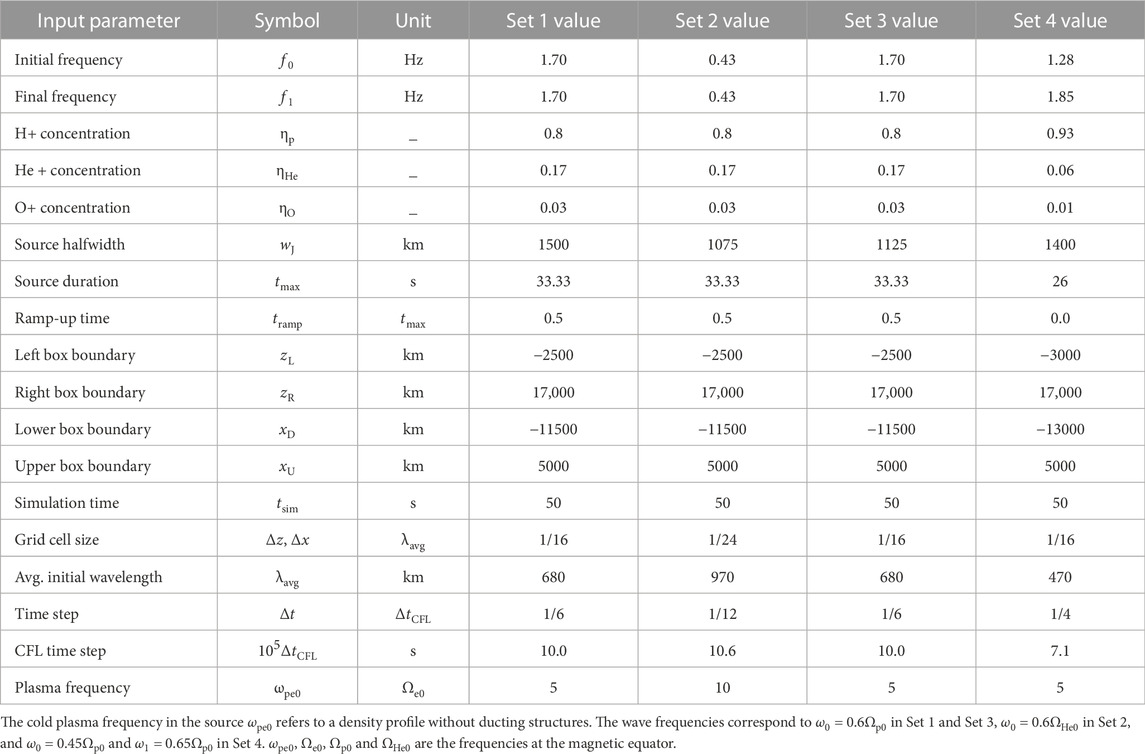
TABLE 1. Four sets of input parameters of four separate simulation runs.

3 Results

3.1 Constant-frequency hydrogen band wave

We first analyze the wave propagation properties of a simple hydrogen band EMIC wave packet with no amplitude modulations and a constant frequency. The corresponding input parameters can be found in Table 1, Set 1. In Figure 1, we plot the total magnetic and electric fields at time t = 25 s along with selected field components. Because the source is symmetric, we will discuss only the waves propagating towards z > 0 (northward); the fields propagating towards z < 0 (southward) quickly enter the damping region near box boundaries and dissipate.

FIGURE 1

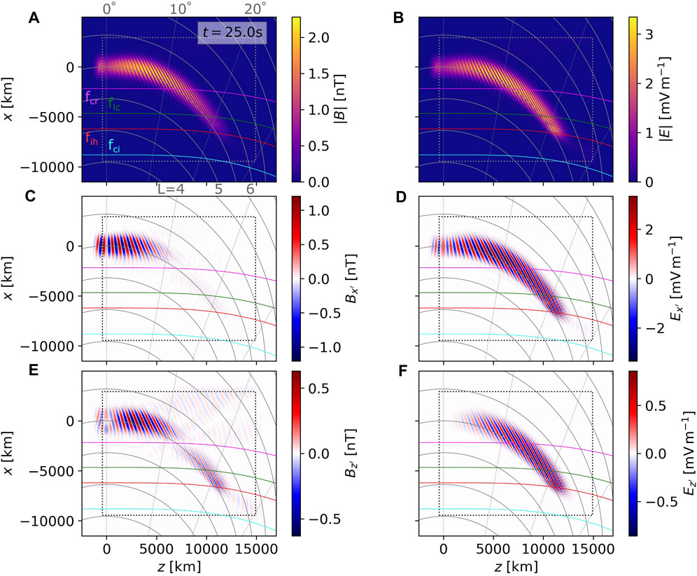
FIGURE 1. Snapshots of magnetic and electric fields from the simulation run with input parameter Set 1 (constant-frequency unducted hydrogen band wave packet with a single amplitude maximum). (A) Amplitude of the wave magnetic field |B|. This panel shows the time stamp t = 25 s, labels of the radial lines of constant latitude, L-shell labels, and characteristic frequency labels: magenta curve for wave frequency encountering the crossover frequency f_cr, green for the L-cutoff frequency f_lc, red for the ion hybrid frequency f_ih, and cyan for the cyclotron frequency f_ci (helium gyrofrequency in this case). The dotted rectangle represents boundaries of the damping region. (B) Amplitude of the wave electric field |E|. (C) Magnetic field component B_x′ perpendicular to the local field line (parallel to the meridional plane). (D) Electric field component E_x′. (E) Magnetic field component B_z′. (F) Electric field component E_z′.

Several important features of unducted EMIC wave propagation can be discerned from these snapshots. The magnetic and electric fields in Figures 1A,B display spatial oscillations with a period of λ_w/2, hinting at a rapid increase in ellipticity away from the source. Highly elliptical polarization suggests oblique wave vector direction, which can be confirmed by observing the angle between wave crests and field lines. When the wave frequency approaches the ion hybrid frequency (represented by the red curves in Figure 1), the magnetic field diminishes, while the electric field remains strong, confirming that the oblique EMIC wave is becoming electrostatic at the hybrid resonance.

The perpendicular component B_x′ plotted in Figure 1C disappears near the crossover frequency (magenta curves) because the wave becomes near linearly polarized with most of its magnetic amplitude in the y′ direction. Because the source width 2w_J is about 4.4 equatorial wavelengths, the plane wave approximation is not heavily violated, and E ⋅B = 0 implies that the B_y′ component will have a spatial distribution similar to E_x′ (Figure 1D).

Figure 1E shows the magnetic field component B_z′, which reveals weak parts of the wave field moving across field lines, deviating from the expected quasi-parallel propagation of energy. Most of these can be shown to be right-handed and are related to mode conversions near characteristic frequencies—they will be described with the help of polarization analysis in the following paragraphs. However, some of these weak R-mode waves originate directly in the source. This observation may seem surprising since the source current density was obtained based on the assumption of a left-handed circular polarization. However, those calculations relied on the plane wave approximation in a homogeneous plasma, which is not exactly satisfied when the source is finite and the electron density in the radial direction changes by about 10% per wavelength. How the finite 1D source affects wave properties can be shown by constructing the magnetic field wave equation from Eqs 1, 2 (dropping the particle species index i)

$\nabla \times \left(\nabla \times \mathit{B}\right)={\mu }_0\nabla \times {\mathit{J}}_{\mathit{s}}-\frac{1}{c^2}\frac{{\partial }^2\mathit{B}}{\partial t^2}.(27)$

The circularly polarized current can be represented by

${\mathit{J}}_{\mathit{s}}=J_{\mathrm{s}0}\left(x\right)\left(\cos \psi ,\sin \psi ,0\right),(28)$

where J_s0(x) represents the amplitude profile. If we take the curl of J_s, we get

$\nabla \times {\mathit{J}}_{\mathit{s}}=\left(J_{\mathrm{s}0}{k}_z\cos \psi ,J_{\mathrm{s}0}{k}_z\sin \psi ,\left(\partial J_{\mathrm{s}0}/\partial x\right)\sin \psi \right).(29)$

The z-component will propagate into the calculation of B and cause deviations from the circular polarization. This behavior is confirmed in Figure 1E, where we show B_z′ to be nonzero in the source for z = 0, x ≠ 0. The resulting wave field can be decomposed into left-hand and right-hand polarized components, and thus the finite source supports both the L-mode and the R-mode. However, because the plane wave approximation is violated only weakly, the corresponding R-mode wave field is also weak. With decreasing w_J, the source is becoming increasingly point-like, supporting radiation in directions far away from θ_k = 0°. For the sake of completeness, we may also construct the electric field wave equation

$-\nabla \times \left(\nabla \times \mathit{E}\right)={\mu }_0\frac{\partial {\mathit{J}}_{\mathit{s}}}{\partial t}+\frac{1}{c^2}\frac{{\partial }^2\mathit{E}}{\partial t^2}.(30)$

The spatial derivatives of current density are not present here; therefore, the electric field component E_z′ remains zero in the source, as documented in Figure 1F.

To better understand the wave propagation and polarization properties, we run SVD analysis on the coarse grid, following the methods described in Section 2.3. The results are shown in Figure 2, using the same snapshot as in Figure 1. Figure 2A presents the Poynting flux amplitude |μ₀S| in units of nT mV⁻¹. The lower threshold for all data is set to 10^−3.5 of the maximum Poynting flux in the chosen snapshot. As expected, the peak energy flux follows the starting field line L = 5.5, with only a slight deviation towards high L-shells, which is further confirmed by the low values of polar angle of the Poynting vector θ_S. The only regions where θ_S becomes large are the reflection region near the hybrid resonance, and the southern hemisphere (which will not be further discussed). Figure 2C shows that the wave starts as near left-hand circularly polarized, then becomes linearly polarized when crossing f = f_cr, and in the reflection region, a mixture of left-hand and right-hand polarization appears. The wave normal angle θ_k in Figure 2D shows a steady increase from near zero in the source up to 90° during reflection. However, the WNA values are somewhat noisy, especially near f_cr, near f_ih, and at the edges of the wave packet. Similar features are displayed by the azimuthal angle ϕ_k in Figure 2E, with the values jumping from 0° to 180°. At the two above-mentioned characteristic frequencies, the B-field polarization ellipse is degenerate (linear polarization), and thus the direction of the wave vector cannot be determined. At the wave packet edges, the variations come from the mixing of L-mode with the very weak R-mode. The planarity stays above 0.7 (Figure 2F), confirming that the use of the SVD analysis is meaningful.

FIGURE 2

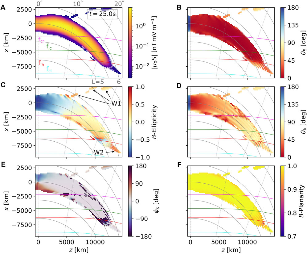
FIGURE 2. Snapshots of wave propagation and polarization properties from Set 1, taken at the same time t = 25 s as the wave fields in Figure 1. The plotted data range has been changed from Figure 1 to exclude the damping region. (A) Magnitude of the Poynting flux. (B) Polar angle of the Poynting vector. (C) Ellipticity of the magnetic field. Labels W1 and W2 point to weaker fields whose propagation properties differ from the main packet. (D) Wave normal angle. (E) Azimuthal angle of the wave vector. (F) Planarity of the magnetic field. All quantities were obtained through SVD methods with spectral averaging over three equatorial wave periods, as described in Section 2.3.

A peculiar behavior can be seen near the source, where the azimuthal angle shows large eastward and westward deviations (Figure 2E). An explanation can be provided through the same calculations that led to Eq. 29. The additional part of the B_z component arising from the ∂/∂x gradient has a phase shift of 90° with respect to B_x, differing from the 180° shift expected in an oblique EMIC plane wave propagating in the meridional plane. This phase difference is demonstrated by Figures 1C,E where B_x′ is almost zero in the source while B_z′ attains its maximum or minimum at the same time. However, as long as the wave normal angle is small, the deviations in ϕ_k have little impact on wave propagation away from the source.

Apart from the main field-aligned packet, weaker fields with an oblique energy propagation direction appear in Figure 2, labeled W1 and W2. The W1 field has both θ_S and θ_k moderately or highly oblique $(>50°)$, is right-hand elliptically polarized, and has origin in the weak R-mode radiated from the source. This origin can be confirmed by looking at B_z′ (Figure 1E) and tracing it back in time. A portion of the W1 field first propagates through the f_cr, experiences polarization reversal, reflects at the L-cutoff, and then goes through a second polarization reversal before arriving at the point of observation. The W2 field has similar properties but shows a smaller obliquity of θ_S and represents waves that were initially quasiparallel, did not experience reflection at the ion hybrid frequency and became unguided.

Neglecting the weak W1 and W2 fields, we may conclude that in a cold plasma with a high He + concentration (17%), an unducted hydrogen band wave that started with low values of WNA near the source will be entirely reflected back to the equator. To further confirm this conclusion, we show the evolution of the wave packet in three snapshots plotted in Figure 3. Figures 3A–F cover the initial stage before reflection, where we can clearly see the W1 field escaping away from L = 5.5 and the main field going through polarization reversal. We skip over the intermediate stage already discussed in Figure 2 and go to the final stage at t = 45 s, where the majority of the wave packet has been reflected. The reflected wave goes through a second polarization reversal and reaches the source region as a very oblique, left-hand highly elliptically polarized EMIC emission. Due to the slight deviation of S from the field-aligned direction, the reflected wave passes above the center of the wave source when it returns to the equatorial plane. A space probe flying through the source region can, therefore, easily miss the reflected wave, depending on the probe’s precise position and velocity. Our results demonstrate that more data from multi-spacecraft observations at close separations are needed to evaluate the occurrence and physical properties of reflected EMIC waves.

FIGURE 3

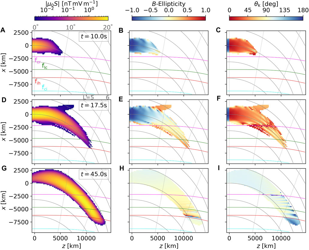
FIGURE 3. Poynting vector magnitude, B-field ellipticity, and wave normal angle calculated for three different snapshots from Set 1: t = 10 s in panels (A–C), t = 17.5 s in panels (D–F), and t = 45.0 s in panels (G–I).

3.2 Constant-frequency helium band wave

In a cold plasma with the three ions H+, He+, and O+, the dispersive properties of the helium band EMIC wave are generally similar to those of the hydrogen band wave, with the most significant difference being in wavenumber. However, because He-band is associated with higher densities (Meredith et al., 2014), even the wavenumbers can be close in value. One clear distinction appears once waves pass through the L-mode stopband: while the H-band waves will encounter another stopband at higher latitudes, the He-band can propagate unimpeded down to ionospheric altitudes. Moreover, low oxygen concentrations in the plasmatrough can push the characteristic frequencies close to Ω_O.

In the simulation run with input parameter Set 2, we choose ω₀/Ω_He0 = 0.6, which is the same value as ω₀/Ω_p0 in Set 1. The plasma frequency is doubled, which still makes the wavelength larger than in the hydrogen band case. Furthermore, the source extent is decreased from ±1,500 km to ±1,075 km. The full source width 2w_J is now only about two equatorial wavelengths, which leads to enhanced radiation in oblique directions. This change in the radiation pattern is demonstrated in Figures 4A,B, where the magnetic field components B_x′ and B_z′ show oblique wave crests emanating from the source. The power of these weak oblique fields is about two orders of magnitude below the peak of the main packet (Figure 4C), making them more significant than in the wide-source case from Figure 2. The polar angle θ_S reveals that some of these weaker waves stay at latitudes below 10°, displaying very oblique propagation of energy, while some are more parallel and quickly (i.e., at time t = 27.5 s) reach latitudes up to above 20°. The first group is marked W1 in Figure 4E and has two components. The outward propagating component is right-hand polarized and quickly reaches the damping boundary—its properties are similar to the W1 field from Figure 2, hence the shared label. The second component propagates inward, experiences polarization reversal, and reflects at the L-cutoff. The second group, labeled W2, propagates in a quasiparallel fashion down to the lower box boundary without experiencing any notable changes in propagation properties, becoming unguided after passing below f_ih. We may notice in Figure 4F that at the boundaries between L-mode-dominated and R-mode-dominated regions, the wave normal angle appears to be near 90°.

FIGURE 4

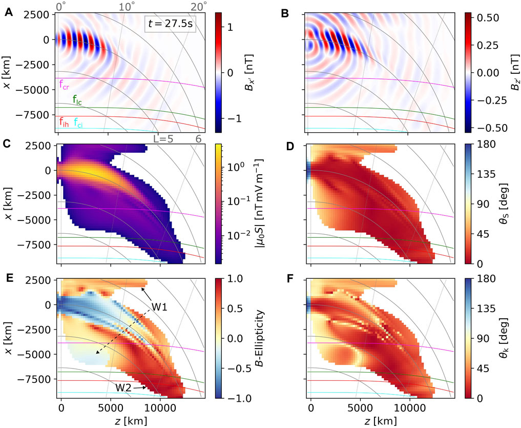
FIGURE 4. Snapshots of wave fields and propagation properties from the simulation run with input parameter Set 2 (constant-frequency unducted helium band wave packet with a single amplitude maximum) taken at t = 27.5 s. (A) Magnetic field component B_x′ perpendicular to the local field line (parallel to the meridional plane). (B) Magnetic field component B_z′. (C) Magnitude of the Poynting flux. (D) Polar angle of the Poynting vector. (E) Ellipticity of the magnetic field. Labels W1 and W2 point to weaker fields whose propagation properties differ from the main packet. (F) Wave normal angle. Note that the colored curves now represent crossings with characteristic frequencies in the helium band, with f_ci standing for the oxygen gyrofrequency.

The narrow source not only affects the amplitude of the weak R-mode, but also changes the propagation properties of the main L-mode packet. This is easier to observe during later times of the wave field evolution, as demonstrated by the three snapshots in Figure 5. At t = 17.5 s (Figures 5A–C), the separation into the main packet and secondary R-mode packets is already clear. At a later time, t = 32.4 s (Figures 5D–F), we notice that a part of the main packet near the bottom edge, labeled W3 in Figure 5E, has a near-circular left-hand polarization and quasiparallel wave vector. In Figures 5G–I (snapshot t = 40.0 s), this W3 field is shown to propagate through the crossover frequency without any significant loss of wave power and remain mostly left-hand polarized, while the more oblique portion of the main wave packet undergoes polarization reversal. However, a small amount of wave energy is transferred into a reflected R-mode component near f = f_cr, labeled W4 in Figure 5H. The above-discussed weak fields W1 and W2 are also marked for comparison with Figure 4.

FIGURE 5

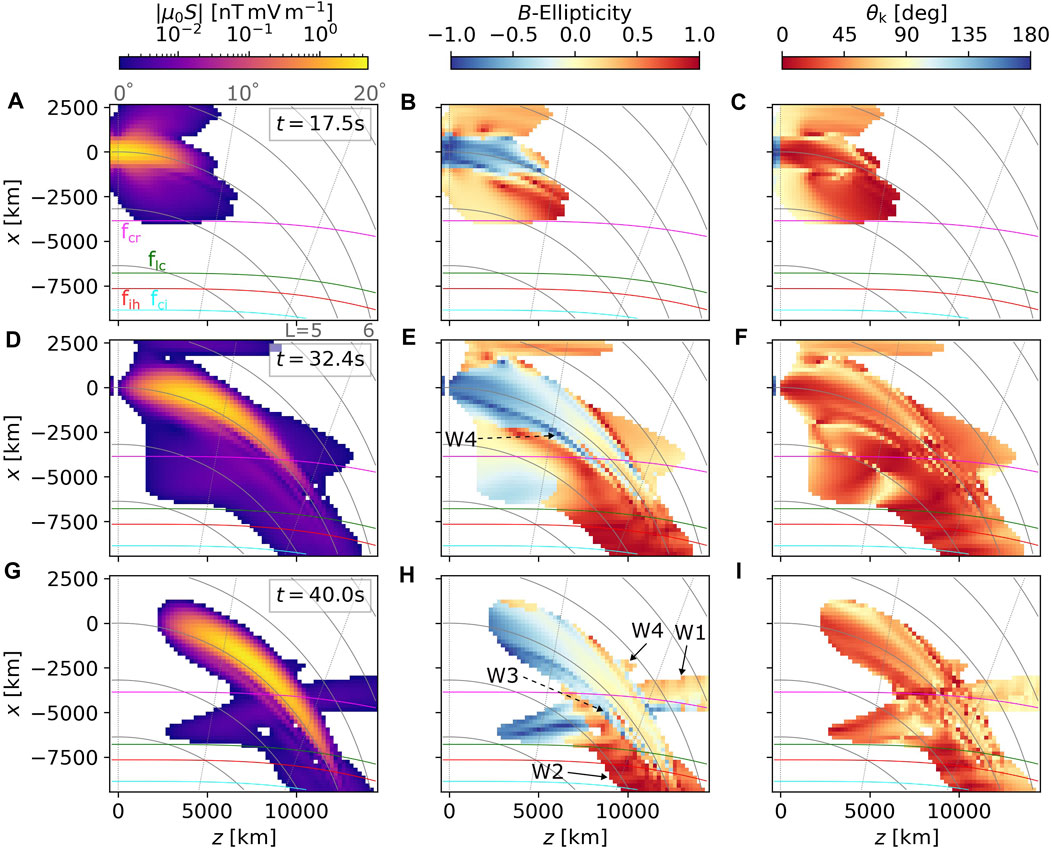
FIGURE 5. Several snapshots of wave propagation properties of the helium band propagation, presented in the same format as the hydrogen band data in Figure 3. (A–C) t = 17.5 s, (D–F) t = 32.4 s, (G–I) t = 40.0 s. Labels, W1, W2, W3, and W4 point to weaker components of the wave field with special propagation and polarization properties.

3.3 Ducted hydrogen band wave

After inspecting the propagation of unducted EMIC waves in Sections 3.1 and Sections 3.2, we turn to ducted propagation on steep density gradients (input parameter Set 3). In this ducted H-band simulation, the source width is smaller than in Set 1, w_J = 1,125 km, but the wavelengths are shorter due to the increased density in the ducting structure. Because of the large radial density gradients, the wavelength in the source cannot be well represented by a single value. Nonetheless, in the chosen setup, the source is still wide enough to emit only negligible power into the oblique directions.

The B_x′ component plotted in Figure 6A shows stark differences from the unducted picture in Figure 1C. When reaching f_cr, the wave crests follow the field line, and the L-value of this field line matches well with the region of steep density drop off (see Figure 6B for a plot of 2D ω_pe/Ω_e0 distribution). As shown in Figures 6C,D, most of the wave power reaches the hybrid resonance and passes towards higher latitudes. However, a significant amount of wave power becomes reflected near the f = f_cr and f = f_lc surfaces. In Figure 6E, we can see that the quasiparallel ducted EMIC wave turns into a mixture of L-mode and R-mode after passing through the crossover. The left-handed part reflects to higher L-shells and goes through a polarization reversal—we label it S3, as it has a similar propagation path to W3, except for being stronger due to ducting. S2’ is an R-mode wave, which has similar properties to the weak field W2 but originates in the polarization reversal instead of being generated directly in the source. Additionally, a weak part of the main packet gets reflected at the crossover and becomes right-hand polarized (W4 in Figure 6E). Due to the mixture of R-mode and L-mode waves with similar power, the wave normal angles plotted in Figure 6F are difficult to interpret, but the quasiparallel component at the center of the wave packet can still be traced.

FIGURE 6

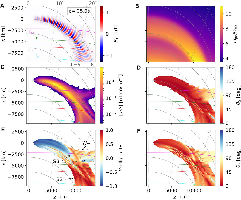
FIGURE 6. Snapshots of wave fields and propagation properties from the simulation run with input parameter Set 3 (constant-frequency ducted hydrogen band wave packet with a single amplitude maximum) taken at t = 35.0 s. Compared to Figure 4, we replaced the B_z′ plot in panel B with a 2D distribution of ω_pe/Ω_e0, which shows the shape of the density structure responsible for guided propagation. The rest of the panels (A−F) show the same type of data as Figure 4. In panel E, certain weak and strong parts of the wave field with special properties are labeled as S2’, S3, and W4.

Values of θ_k below the f = f_ih surface suggest moderate obliquity, which means that these waves are decoupled from the R-mode at ω < Ω_O, and most of their energy will be reflected before reaching low altitudes. However, the simulation would give nearly identical results for He-band with a similar wavenumber (requiring a high-density background), up to minor differences related to the ion composition. The S2’ wave field would then propagate through down to the ionosphere.

3.4 Rising-tone hydrogen band wave

In the previous sections, the current density source was not dynamic, except for the slow changes in amplitude that formed the single-peaked wave packet envelope. We now modulate the wave field into four subpackets and introduce a constant frequency chirp from the initial frequency ω₀ = 0.45Ω_p0 to the final frequency ω₁ = 0.65Ω_p0. As listed in Table 1, the concentration of He+ and O+ has been decreased to prevent the f₀ = f_cr surface from crossing the source. The source width is very slightly (by $\sim 7\%$) smaller than in Set 1 and the initial wavelength is larger, making the source relatively more narrow. This can be noticed in the B_y′ plot in Figure 7A, where a weak quasiparallel field appears at the inner edge of the wave field. In Figure 7B, we show the instantaneous frequency at time t = 15 s, shortly before the reflection of the first subpacket at the hybrid resonance. At the local minimum between the first and second subpacket, which is located near 10° of latitude, the frequency can be seen to have a localized decrease, despite the linearly rising frequency of the source. These are the effects of group velocity dispersion consistent with ∂V_g/∂ω < 0, which have been previously discussed in the context of rising-tone chorus elements by Hanzelka and Santolík (2022).

FIGURE 7

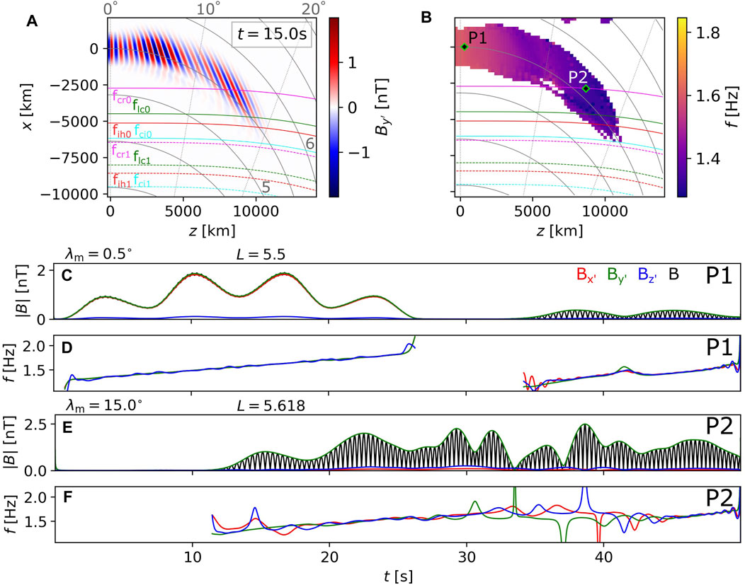
FIGURE 7. Field components and propagation properties of waves from simulation run with input parameter Set 4 (rising-tone unducted hydrogen band wave packet with four subpackets). (A) Magnetic field component B_x′ perpendicular to the local field line (perpendicular to the meridional plane). Snapshot taken at t = 15 s. Crossings of characteristic frequencies for wave at frequency ω₀ are represented by solid lines as before, and the crossing for the final frequency ω₁ are plotted with dashed lines. (B) Instantaneous wave frequency snapshot, obtained as a power-weighted average of frequencies of the three magnetic components. Labels P1 and P2 show positions of probes that collected data analyzed in the following panels and in Figure 8C Probe P1 measured amplitude envelopes of the magnetic field components B_x′, B_y′, and B_z′ plotted in red, green, and blue, respectively. The total magnetic field |B| is plotted with a black line. (D) Instantaneous frequencies from Probe P1, color coded as in the previous panel. (E, F) Same as panels (C, D), but with data from probe P2.

To provide another view on the evolution of wave frequency and the effects of reflected waves, we process data from two selected simulation probes, P1 and P2, whose position is shown in Figure 7B (P1 near the source, P2 at the f_cr crossing of the first subpacket). Unlike in the presentation of the constant-frequency wave propagation (Section 3.1), we can show the whole time evolution in one plot, but we are limited to a single point in space. Figure 7C presents the amplitude envelopes of all three magnetic field components B_x′, B_y′, and B_z′, as well as the total magnetic field |B|. Before t ∼ 30 s, the four northward propagating subpackets have a negligible parallel component, and the peak amplitude is near equal to B₀/100, as dictated by the source properties. The two perpendicular components have similar magnitudes, suggesting circular polarization, which is further confirmed by the negligible oscillations in |B|. After t ∼ 30 s, the reflected wave packet passes over probe P1, but its amplitude is diminished, with the second subpacket having less than 15% of its original amplitude. The B_y′ component dominates, and |B| exhibits strong oscillations at two times the wave frequency, which are signs of linear polarization and high obliquity in the hydrogen band L-mode. The frequencies near the source (Figure 7D) are linearly growing, except for minor oscillations in the frequency derived from B_z′. The chirp rate within subpackets of the reflected wave is higher than the initial value, which is again the effect of group velocity dispersion that we already noted when describing Figure 7B.

Moving to probe P2, we observe the behavior of two linearly polarized waves propagating in opposite directions. This overlap creates multiple very short subpackets associated with large variations in the instantaneous frequency. When such a structure is observed, we must separate the two modes, either by the Hilbert-Huang transform (HHT; for an application on EMIC waves, see (Ojha et al., 2021)) or by inspection of time-frequency spectrograms. We choose the latter method and plot spectrograms of power spectral density (PSD) and propagation properties in Figure 8. The PSD near equator, as shown in Figure 8A, confirms that the reflected emission has a considerably lower power (down by almost two orders of magnitude) than the forward propagating wave. Depending on the signal-to-noise ratio of the original wave packet, only parts of the reflected riser may be visible, or none at all. It is of note that the rising-tone element has a considerable spectral width, which is the consequence of the Fourier uncertainty principle for short wave packets. Even with the 93.75% overlap of the STFT time windows, the frequency resolution is too low to determine whether the individual subpackets are chirping—the line plots obtained from Hilbert transform are better suited for this purpose but might require some form of mode decomposition like the one included within HHT. Figure 8 supports our previous assessment of the reflected wave’s propagation properties, clearly showing the near-linear polarization and highly oblique wave normal angle.

FIGURE 8

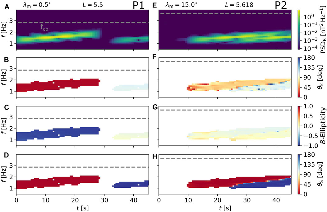
FIGURE 8. Time-frequency spectrograms constructed from time series of wave magnetic field captured by probes P1 (A–D) and P2 (E–H) placed inside the rising-tone EMIC wave field. (A) Magnetic field power spectral density, with the dashed grey line representing the local proton gyrofrequency. (B) Wave normal angle. (C) Ellipticity of the magnetic field. (D) Polar angle of the Poynting vector. (E–H) Same as panels (A–D), but with data from probe P2.

Finally, Figures 8E–H show spectrograms constructed from the probe P2 data. Due to the close frequencies of the two wave packets, it is not immediately clear from the power spectrum in Figure 8E that we are indeed observing two risers propagating in opposite directions. Fortunately, the polar angle θ_S in Figure 8H shows a clear division into two northward and southward propagating elements. Figures 8F,G further show that one element has θ_k about 65° and ellipticty of −0.2, while the other has θ_k ≈ 100° and positive ellipticity $<0.1$ (these values slightly differ between subpackets). However, in practical applications with the presence of noise, these small differences in WNA and ellipticity could not serve as reliable criteria, and the Poynting flux data would be needed. Before we conclude this section, we must note that the probe P2 was shifted to a slightly higher L-shell than P1 to ensure similar wave powers of the forward-propagating and reflected element—a property that is not necessarily satisfied within real spacecraft data.

4 Discussion

The results of constant-frequency wave simulations from Section 3.1 can be compared to the 2D finite-element method (FEM) simulations of hydrogen band EMIC waves conducted by Kim and Johnson (2016). The FEM approach is used to solve Maxwell equations as a boundary value problem, with the result being the spatial distribution of eigenmodes (Fourier space solutions). This approach differs from our initial value problem, but the fixed frequency and slowly changing source amplitude allow for a meaningful comparison. Kim and Johnson (2016) show that with a wide source region (about four equatorial wavelengths, similar to our Set 1), the wave propagation is initially nearly parallel but becomes significantly oblique before encountering the crossover frequency. Most of those waves reflect at the hybrid resonance after going through polarization reversal, with only a negligible amount passing through to lower altitudes. This weak wave that does not experience reflection corresponds to our W2 field in Figure 2. The R-mode wave W1 emanating from the source was not clearly detected in the FEM simulations, likely because of a stricter power threshold. Due to different ion compositions and density models, the reflected wave in the FEM simulation went to a higher L-shell than in our case and quickly encountered an absorbing boundary, so its propagation properties were not analyzed.

Kim and Johnson (2016) further analyzed a propagation scenario with a very narrow source, which can be compared to our Set 2. As in the previous case, the W1 field is not very apparent in the FEM simulation—it is possible that differences in the initialization (1D current density source in contrast to a 2D electric field source) are behind this disagreement. What the simulations agree on is the presence of a quasiparallel L-mode component at the inner edge of the wave packet (W3 in Figure 5). Some of these left-handed waves preserve their polarization and continue to f_lc, while some reflect at f_cr and become right-handed (W4 in Figure 5A in Figure 4 of Kim and Johnson (2016)). Unlike in the FEM simulation, the dispersion of R-mode at f_ih is unclear due to the overlap with the weak field W2, which originates in the narrow source. We must also point out that we simulated a helium band wave in Set 2, in contrast to the hydrogen band wave in the FEM simulation, so the comparison can be only qualitative. In qualitative terms, the polarization reversal and mode conversion observed near f = f_cr in our simulations also agree with the theoretical and numerical full-wave analysis conducted by Johnson and Cheng (1999) and Johnson et al. (1995).

The 2D FDTD full-wave simulations of EMIC propagation on a steep density gradient (Figure 6) are, to our knowledge, unique and cannot be directly compared to previous literature. de Soria-Santacruz et al. (2013) performed hot plasma ray tracing simulations in field-aligned density irregularities, showing that density enhancements can guide quasiparallel waves. However, the widths of those enhancements (minimum to minimum) were $\sim 2500\mathrm{k}\mathrm{m}$ and $\sim 625\mathrm{k}\mathrm{m}$, with typical wavelengths ranging from 500 km to 800 km. Under such conditions, the changes in density gradients over a single wavelength are significant, and the plane wave approximation inherent to ray tracing cannot accurately predict wave propagation properties. Furthermore, ray simulations cannot be used to inspect wave energy flow during mode conversion and tunneling. In the full-wave simulation we presented in Figure 6, the H-band EMIC waves guided on the outer edge of a density enhancement are partly reflected on the L-cutoff and partly continue as the quasiparallel R-mode that propagates to lower altitudes. This behavior is similar to the case analyzed by Kim and Johnson (2016) where a moderately oblique wave (θ_k ≈ 40°) launched from the equator partly converts to R-mode and avoids reflection at the hybrid resonance. The ducted mode seems to be more efficient at carrying wave energy to lower altitudes, but this is expected to depend on the exact density model and input wave parameters.

The R-mode waves which penetrated through the f = f_ih surface (see the bottom right corner of Figure 6F) are shown to have a broad range of propagation directions. Extending the simulation box down to the ionosphere is beyond our current computational possibilities, but we may assume that a portion of wave energy will be further guided along the gradient, and another portion will propagate towards lower L-shells. The former can be linked to observations of R-mode waves in the 0.1 − 1.0 Hz range made by the LEO (Low Earth Orbit) satellite DEMETER above and at the ionospheric trough (Parrot et al., 2014). Ducting along the outer edge of plasmaspheric plumes could also explain why the majority of hydrogen band EMIC observed by Polar (Bräysy and Mursula, 2001) and GOES satellites (Noh et al., 2022) are also detected at conjugate ground stations. Another analysis of DEMETER data by Píša et al. (2015) revealed the presence of 1 − 15 Hz R-mode waves at very low L-shells and linked them to He-band EMIC waves. Assuming a strong plasmasphere compression, He-band waves generated at the plasmapause (Fraser and Nguyen, 2001) will fit into this frequency range; therefore, the unguided waves from our ducted simulation can be linked to these observations. We must note that while our density enhancement model was presented as a plume model, the waves never reached its inner boundary, and so it can be seen as a plasmapause model as well.

As far as we know, the 2D full-wave EMIC rising-tone simulations presented in Figures 7, 8 are also unique. Due to the time-dependent nature of the source, such simulations must be performed in the time domain, precluding comparison with FEM models (Kim and Johnson, 2016; 2023). Unlike in the chorus rising-tone simulations of Hanzelka and Santolík (2022), small-scale density irregularities $(\sim 1-100\mathrm{k}\mathrm{m})$ can be neglected since waveguide modes of structures with sizes far below a single wavelength will not be excited (Zudin et al., 2019). Moreover, Landau damping of oblique EMIC waves is typically very weak (Thorne and Horne, 1992), and so it is meaningful to use cold plasma approximation to study unducted wave propagation and reflections, as long as we neglect the impact of warm ions on the dispersive properties near characteristic frequencies (Chen et al., 2011). The spectra of the forward-propagating and reflected risers in Figure 8 can be compared to the spectral analysis of reflected EMIC risers found in Cluster spacecraft data by Grison et al. (2016). The wave normal angles are nearly perpendicular in both cases and the reflected wave power is observed to be slightly reduced. However, while the direction of the Poynting vector in the simulation is nearly parallel (or anti-parallel), the Cluster observations show angles within a 70°–110° interval. Such conditions are possible only when f < f_ih (unguided waves; compare with Supplementary Figure S1C in the Supplementary Material), suggesting that the waves are reflecting slightly below the f = f_ih surface. Thus, despite the similarity in spectra, we are observing a different type of reflection. The importance of unguided waves for propagation of EMIC energy down to the ionosphere has been studied numerically by Pakhotin et al. (2022) using sources at lower L-shells (L = 3.3).

The simulated propagation properties of ducted and unducted EMIC waves can be used to draw conclusions about wave-particle interactions and scattering of resonant electrons and protons. In all unducted cases, the waves become moderately oblique (WNA around 40° and higher) before reaching λ = 10°. Thus the high-order cyclotron resonances (Ma et al., 2019), fractional resonances (Hanzelka et al., 2023), and the Landau resonance (Cao et al., 2019) can become efficient before the wave encounters the crossover frequency. On the other hand, ducted waves remain quasiparallel up to λ > 20°, keeping the first-order cyclotron resonance as the dominant cause of scattering. However, since the L-mode typically cannot pass through the L-cutoff and ω_pe/Ω_e decreases with increasing latitude, interactions with $\sim 1$ MeV and sub-MeV electrons will be limited to the near-equatorial region, where the resonance energy reaches its lowest values.

Last but not least, we should discuss some of the choices made when developing our 2D FDTD simulation code and possible subsequent limitations. The restriction to a cold plasma medium results in the lack of a feedback loop between waves and resonant particles. This limitation is especially noticeable in studies of rising-tone EMIC emissions, which are generated by resonant currents formed through nonlinear processes. These currents have an impact on wave properties during propagation in the near-equatorial region and can be properly captured only by including the hot plasma component (Shoji and Omura, 2013; Denton et al., 2019). Another choice affecting the core of the simulation code is the initialization of the wave field. While some authors prefer to initialize the simulation with an electric (Streltsov et al., 2006; Kim and Johnson, 2016) or magnetic field (Xu et al., 2020), others feed current into the simulation box, which then generates the waves (Hosseini et al., 2021; Hanzelka and Santolík, 2022; Pakhotin et al., 2022). The initialization with magnetic field is likely the most straightforward, but we consider the initialization with current density to be more natural, as it resembles wave growth due to hot plasma current. Reduction of the source to one dimension requires the use of an additional numerical factor (Eq. 18), but it removes the need to estimate the unknown field-aligned extent of the source, and it dramatically decreases the size of the input data for time-dependent sources (instead of two spatial dimensions and one temporal, we have only one spatial and one temporal). The deviations from the meridional plane shown in Figure 2E cannot be adequately studied and addressed in a 2D simulation. Implementing a 3D FDTD solver would not be difficult, and it would allow us to construct realistic models of density ducts. Unfortunately, memory constraints would prevent the investigation of wave propagation further away from the equator, where the mode conversion and polarization reversals occur. Adopting spherical coordinates as done by Xu et al. (2020) or Pakhotin et al. (2022) would reduce the box size in cases of field-aligned propagation, boosting the performance in both 2D and 3D simulations, but would not be very beneficial when studying duct leakages and unguided waves. 3D Ray tracing codes thus remain the best method for studies of azimuthal propagation of EMIC waves (Xiao et al., 2012; Chen et al., 2014; Santolík et al., 2016; Hanzelka et al., 2022).

5 Conclusion

The results presented in this paper can be summarized into five points:

1. Two-dimensional finite-difference time-domain simulations can be efficiently used to simulate the propagation of EMIC wave fields generated by time-varying sources in the magnetosphere.

2. Simulated mode conversions and wave reflections corroborate the previous results of Kim and Johnson (2016). Namely, we observed polarization reversal and mode conversions near the crossover frequency, and reflections at the L-cutoff and ion hybrid resonance.

3. A finite and narrow 1D source of left-hand polarized current produces not only a quasiparallel L-mode wave, but also weak R-mode waves propagating into a wide range of directions.

4. Density gradients at the outer edge of plasmaspheric plumes (or plasmapause) can guide wave energy to high latitudes and are a strong candidate for explaining frequent observations of EMIC waves at low altitudes. On the other hand, unducted waves quickly become oblique and experience reflection at the ion hybrid resonance after going through a polarization reversal.

5. Reflected rising-tone EMIC emissions can be observed when the probes are fortuitously positioned, but the propagation properties in our simulation differ from those in Cluster observations of reflected waves (Grison et al., 2016).

We have shown four different scenarios of EMIC wave propagation (unducted H-band, unducted He-band, ducted H-band, unducted rising-tone H-band), but we have not studied the sensitivity of our results to changes in input parameters. A sampling of initial wave frequencies and cold plasma densities could be used to investigate the wave distribution during different geomagnetic conditions. The numerical code also has capabilities to simulate the effects of spatial variability in ion concentrations (Min et al., 2015), branch splitting by minority ions (Miyoshi et al., 2019), falling-tone triggered emissions (Nakamura et al., 2016), propagation of waves generated by an oblique source, spreading of short EMIC pulses, and many other concepts that were before thoroughly investigated with 2D FDTD numerical models. Furthermore, the resulting wave fields can be used as an input in test-particle simulations to study the scattering and precipitation of energetic ions and relativistic electrons. These topics will be investigated in our future research.

Data availability statement

The datasets presented in this study can be found in online repositories. The names of the repository/repositories and accession number(s) can be found below: https://figshare.com/s/9d05a8bf0646fdceac8a.

Author contributions

MH created the full-wave simulation code, analyzed the resulting simulated wave fields, and wrote the original manuscript. WL secured the funding. MH and WL initiated the study. WL, QM, and MQ provided consultations on EMIC wave propagation properties based on experimental observations. LC, X-CS, and LG provided helpful comments during the course of the project. All authors contributed to the article and approved the submitted version.

Funding

The research at Boston University is supported by NASA grants 80NSSC20K0698, 80NSSC20K1270, and 80NSSC21K1312, as well as the NSF grant AGS-2019950. QM would like to acknowledge the NASA grant 80NSSC20K0196 and the NSF grant AGS-2225445. LG gratefully acknowledges the NASA FINESST grant 80NSSC20K1506.

Conflict of interest

The authors declare that the research was conducted in the absence of any commercial or financial relationships that could be construed as a potential conflict of interest.

Publisher’s note

All claims expressed in this article are solely those of the authors and do not necessarily represent those of their affiliated organizations, or those of the publisher, the editors and the reviewers. Any product that may be evaluated in this article, or claim that may be made by its manufacturer, is not guaranteed or endorsed by the publisher.

Supplementary material

The Supplementary Material for this article can be found online at: https://www.frontiersin.org/articles/10.3389/fspas.2023.1251563/full#supplementary-material

References

Allen, R. C., Zhang, J. C., Kistler, L. M., Spence, H. E., Lin, R. L., Klecker, B., et al. (2015). A statistical study of EMIC waves observed by cluster: 1. Wave properties. J. Geophys. Res. Space Phys. 120, 5574–5592. doi:10.1002/2015JA021333

CrossRef Full Text | Google Scholar

Anderson, B. J., Denton, R. E., Ho, G., Hamilton, D. C., Fuselier, S. A., and Strangeway, R. J. (1996). Observational test of local proton cyclotron instability in the Earth’s magnetosphere. J. Geophys. Res. 101, 21527–21543. doi:10.1029/96JA01251

CrossRef Full Text | Google Scholar

Angerami, J. J. (1970). Whistler duct properties deduced from VLF observations made with the Ogo 3 satellite near the magnetic equator. J. Geophys. Res. 75, 6115–6135. doi:10.1029/JA075i031p06115

CrossRef Full Text | Google Scholar

Baker, D. N. (2021). Wave-particle interaction effects in the Van Allen belts. Earth Planets Space 73, 189. doi:10.1186/s40623-021-01508-y

PubMed Abstract | CrossRef Full Text | Google Scholar

Bortnik, J., Albert, J. M., Artemyev, A., Li, W., Jun, C.-W., Grach, V. S., et al. (2022). Amplitude dependence of nonlinear precipitation blocking of relativistic electrons by large amplitude EMIC waves. Geophys. Res. Lett. 49, e2022GL098365. doi:10.1029/2022GL098365

PubMed Abstract | CrossRef Full Text | Google Scholar

Bräysy, T., and Mursula, K. (2001). Conjugate observations of electromagnetic ion cyclotron waves. J. Geophys. Res. 106, 6029–6041. doi:10.1029/2000JA003009

CrossRef Full Text | Google Scholar

Bräysy, T., Mursula, K., and Marklund, G. (1998). Ion cyclotron waves during a great magnetic storm observed by Freja double-probe electric field instrument. J. Geophys. Res. 103, 4145–4155. doi:10.1029/97JA02820

CrossRef Full Text | Google Scholar

Cao, X., Ni, B., Summers, D., Shprits, Y. Y., Gu, X., Fu, S., et al. (2019). Sensitivity of EMIC wave-driven scattering loss of ring current protons to wave normal angle distribution. Geophys. Res. Lett. 46, 590–598. doi:10.1029/2018GL081550

CrossRef Full Text | Google Scholar

Chen, H., Gao, X., Lu, Q., and Wang, S. (2019a). Analyzing EMIC waves in the inner magnetosphere using long-term van allen probes observations. J. Geophys. Res. (Space Phys. 124, 7402–7412. doi:10.1029/2019JA026965

CrossRef Full Text | Google Scholar

Chen, L., Jordanova, V. K., Spasojević, M., Thorne, R. M., and Horne, R. B. (2014). Electromagnetic ion cyclotron wave modeling during the geospace environment modeling challenge event. J. Geophys. Res. Space Phys. 119, 2963–2977. doi:10.1002/2013JA019595

CrossRef Full Text | Google Scholar

Chen, L., Thorne, R. M., and Bortnik, J. (2011). The controlling effect of ion temperature on EMIC wave excitation and scattering. Geophys. Res. Lett. 38, L16109. doi:10.1029/2011GL048653

CrossRef Full Text | Google Scholar

Chen, L., Thorne, R. M., and Horne, R. B. (2009). Simulation of EMIC wave excitation in a model magnetosphere including structured high-density plumes. J. Geophys. Res. Space Phys. 114, A07221. doi:10.1029/2009JA014204

CrossRef Full Text | Google Scholar

Chen, L., Thorne, R. M., Jordanova, V. K., Wang, C.-P., Gkioulidou, M., Lyons, L., et al. (2010). Global simulation of EMIC wave excitation during the 21 April 2001 storm from coupled RCM-RAM-HOTRAY modeling. J. Geophys. Res. Space Phys. 115, A07209. doi:10.1029/2009JA015075

CrossRef Full Text | Google Scholar

Chen, L., Zhu, H., and Zhang, X. (2019b). Wavenumber analysis of EMIC waves. Geophys. Res. Lett. 46, 5689–5697. doi:10.1029/2019GL082686

CrossRef Full Text | Google Scholar

Cornwall, J. M., Coroniti, F. V., and Thorne, R. M. (1970). Turbulent loss of ring current protons. J. Geophys. Res. 75, 4699–4709. doi:10.1029/JA075i025p04699

CrossRef Full Text | Google Scholar

Cornwall, J. M. (1965). Cyclotron instabilities and electromagnetic emission in the ultra low frequency and very low frequency ranges. J. Geophys. Res. 70, 61–69. doi:10.1029/JZ070i001p00061

CrossRef Full Text | Google Scholar

Denton, R. E., Goldstein, J., Menietti, J. D., and Young, S. L. (2002). Magnetospheric electron density model inferred from Polar plasma wave data. J. Geophys. Res. Space Phys. 107, 1386. doi:10.1029/2001JA009136

CrossRef Full Text | Google Scholar

Darrouzet, F., Gallagher, D. L., André, N., Carpenter, D. L., Dandouras, I., Décréau, P. M. E., et al. (2009). Plasmaspheric density structures and dynamics: properties observed by the CLUSTER and IMAGE missions. Space Sci. Rev. 145, 55–106. doi:10.1007/s11214-008-9438-9

CrossRef Full Text | Google Scholar

de Soria-Santacruz, M., Spasojevic, M., and Chen, L. (2013). EMIC waves growth and guiding in the presence of cold plasma density irregularities. Geophys. Res. Lett. 40, 1940–1944. doi:10.1002/grl.50484

CrossRef Full Text | Google Scholar

Denton, R. E., Menietti, J. D., Goldstein, J., Young, S. L., and Anderson, R. R. (2004). Electron density in the magnetosphere. J. Geophys. Res. Space Phys. 109, A09215. doi:10.1029/2003JA010245

CrossRef Full Text | Google Scholar

Denton, R. E., Ofman, L., Shprits, Y. Y., Bortnik, J., Millan, R. M., Rodger, C. J., et al. (2019). Pitch angle scattering of sub-MeV relativistic electrons by electromagnetic ion cyclotron waves. J. Geophys. Res. Space Phys. 124, 5610–5626. doi:10.1029/2018JA026384

CrossRef Full Text | Google Scholar

Engebretson, M. J., Posch, J. L., Wygant, J. R., Kletzing, C. A., Lessard, M. R., Huang, C. L., et al. (2015). Van Allen probes, NOAA, GOES, and ground observations of an intense EMIC wave event extending over 12 h in magnetic local time. J. Geophys. Res. Space Phys. 120, 5465–5488. doi:10.1002/2015JA021227

CrossRef Full Text | Google Scholar

Fraser, B. J., and Nguyen, T. S. (2001). Is the plasmapause a preferred source region of electromagnetic ion cyclotron waves in the magnetosphere? J. Atmos. Sol.-Terr. Phys. 63, 1225–1247. doi:10.1016/S1364-6826(00)00225-X

CrossRef Full Text | Google Scholar

Gedney, S. D. (2011). Introduction to the finite-difference time-domain (FDTD) Method for electromagnetics. Synthesis lectures on computational electromagnetics. Morgan & Claypool Publishers. doi:10.2200/S00316ED1V01Y201012CEM027

CrossRef Full Text | Google Scholar

Grach, V. S., and Demekhov, A. G. (2020). Precipitation of relativistic electrons under resonant interaction with electromagnetic ion cyclotron wave packets. J. Geophys. Res. Space Phys. 125, e27358. doi:10.1029/2019JA027358

CrossRef Full Text | Google Scholar

Grison, B., Darrouzet, F., Santolík, O., Cornilleau-Wehrlin, N., and Masson, A. (2016). Cluster observations of reflected EMIC-triggered emission. Geophys. Res. Lett. 43, 4164–4171. doi:10.1002/2016GL069096

CrossRef Full Text | Google Scholar

Grison, B., Hanzelka, M., Breuillard, H., Darrouzet, F., Santolík, O., Cornilleau-Wehrlin, N., et al. (2018). Plasmaspheric plumes and EMIC rising tone emissions. J. Geophys. Res. Space Phys. 123, 9443–9452. doi:10.1029/2018JA025796

CrossRef Full Text | Google Scholar

Gurnett, D. A., and Bhattacharjee, A. (2017). Introduction to plasma Physics: With space, laboratory and astrophysical applications. Cambridge University Press.

Google Scholar

Horne, R. B., and Thorne, R. M. (1993). On the preferred source location for the convective amplification of ion cyclotron waves. J. Geophys. Res. 98, 9233–9247. doi:10.1029/92JA02972

CrossRef Full Text | Google Scholar

Hanzelka, M., Li, W., and Ma, Q. (2023). Parametric analysis of pitch angle scattering and losses of relativistic electrons by oblique EMIC waves. Front. Astronomy Space Sci. 10, 1163515. doi:10.3389/fspas.2023.1163515

CrossRef Full Text | Google Scholar

Hanzelka, M., Němec, F., Santolík, O., and Parrot, M. (2022). Statistical analysis of wave propagation properties of equatorial noise observed at low altitudes. J. Geophys. Res. Space Phys. 127, e30416. doi:10.1029/2022JA030416

CrossRef Full Text | Google Scholar

Hanzelka, M., and Santolík, O. (2022). Effects of field-aligned cold plasma density filaments on the fine structure of chorus. Geophys. Res. Lett. 49, e2022GL101654. doi:10.1029/2022GL101654

CrossRef Full Text | Google Scholar

Horne, R. B., and Miyoshi, Y. (2016). Propagation and linear mode conversion of magnetosonic and electromagnetic ion cyclotron waves in the radiation belts. Geophys. Res. Lett. 43, 039. doi:10.1002/2016GL070216

CrossRef Full Text | Google Scholar

Horne, R. B., and Thorne, R. M. (1998). Potential waves for relativistic electron scattering and stochastic acceleration during magnetic storms. Geophys. Res. Lett. 25, 3011–3014. doi:10.1029/98GL01002

CrossRef Full Text | Google Scholar

Hosseini, P., Agapitov, O., Harid, V., and Gołkowski, M. (2021). Evidence of small scale plasma irregularity effects on whistler mode chorus propagation. Geophys. Res. Lett. 48, e92850. doi:10.1029/2021GL092850

CrossRef Full Text | Google Scholar

Hu, Y., Denton, R. E., and Johnson, J. R. (2010). Two-dimensional hybrid code simulation of electromagnetic ion cyclotron waves of multi-ion plasmas in a dipole magnetic field. J. Geophys. Res. Space Phys. 115, A09218. doi:10.1029/2009JA015158

CrossRef Full Text | Google Scholar

Hu, Y., and Denton, R. E. (2009). Two-dimensional hybrid code simulation of electromagnetic ion cyclotron waves in a dipole magnetic field. J. Geophys. Res. Space Phys. 114, A12217. doi:10.1029/2009JA014570

CrossRef Full Text | Google Scholar

Johnson, J. R., Chang, T., and Crew, G. B. (1995). A study of mode conversion in an oxygen-hydrogen plasma. Phys. Plasmas 2, 1274–1284. doi:10.1063/1.871339

CrossRef Full Text | Google Scholar

Johnson, J. R., and Cheng, C. Z. (1999). Can ion cyclotron waves propagate to the ground? Geophys. Res. Lett. 26, 671–674. doi:10.1029/1999GL900074

CrossRef Full Text | Google Scholar

Jordanova, V. K., Farrugia, C. J., Thorne, R. M., Khazanov, G. V., Reeves, G. D., and Thomsen, M. F. (2001). Modeling ring current proton precipitation by electromagnetic ion cyclotron waves during the May 14-16, 1997, storm. J. Geophys. Res. 106, 7–22. doi:10.1029/2000JA002008

CrossRef Full Text | Google Scholar

Jun, C.-W., Miyoshi, Y., Kurita, S., Yue, C., Bortnik, J., Lyons, L., et al. (2021). The characteristics of EMIC waves in the magnetosphere based on the van allen probes and arase observations. J. Geophys. Res. Space Phys. 126, e29001. doi:10.1029/2020JA029001

CrossRef Full Text | Google Scholar

Kersten, T., Horne, R. B., Glauert, S. A., Meredith, N. P., Fraser, B. J., and Grew, R. S. (2014). Electron losses from the radiation belts caused by EMIC waves. J. Geophys. Res. Space Phys. 119, 8820–8837. doi:10.1002/2014JA020366

CrossRef Full Text | Google Scholar

Kim, E.-H., and Johnson, J. R. (2016). Full-wave modeling of EMIC waves near the He⁺ gyrofrequency. Geophys. Res. Lett. 43, 13–21. doi:10.1002/2015GL066978

CrossRef Full Text | Google Scholar

Kim, E.-H., and Johnson, J. R. (2023). Magnetic tilt effect on externally driven electromagnetic ion cyclotron (EMIC) waves. Geophys. Res. Lett. 50, e2022GL101544. doi:10.1029/2022GL101544

CrossRef Full Text | Google Scholar

Koons, H. C. (1989). Observations of large-amplitude, whistler mode wave ducts in the outer plasmasphere. J. Geophys. Res. 94, 15393–15397. doi:10.1029/JA094iA11p15393

CrossRef Full Text | Google Scholar

Lee, J. H., Blum, L. W., Chen, L., and Kwon, Y. J. (2021). Relationship between muscle mass and non-alcoholic fatty liver disease. Front. Astron. Space Sci. 8, 122. doi:10.3390/biology10020122

CrossRef Full Text | Google Scholar

Li, W., and Hudson, M. K. (2019). Earth’s van allen radiation belts: from discovery to the van allen probes era. J. Geophys. Res. Space Phys. 124, 8319–8351. doi:10.1029/2018JA025940

CrossRef Full Text | Google Scholar

Lyu, X., Ma, Q., Tu, W., Li, W., and Capannolo, L. (2022). Modeling the simultaneous dropout of energetic electrons and protons by EMIC wave scattering. Geophys. Res. Lett. 49, e2022GL101041. doi:10.1029/2022GL101041

CrossRef Full Text | Google Scholar

Ma, Q., Li, W., Yue, C., Thorne, R. M., Bortnik, J., Kletzing, C. A., et al. (2019). Ion heating by electromagnetic ion cyclotron waves and magnetosonic waves in the Earth’s inner magnetosphere. Geophys. Res. Lett. 46, 6258–6267. doi:10.1029/2019GL083513

CrossRef Full Text | Google Scholar

Meredith, N. P., Horne, R. B., Kersten, T., Fraser, B. J., and Grew, R. S. (2014). Global morphology and spectral properties of EMIC waves derived from CRRES observations. J. Geophys. Res. Space Phys. 119, 5328–5342. doi:10.1002/2014JA020064

CrossRef Full Text | Google Scholar

Meredith, N. P., Horne, R. B., Thorne, R. M., and Anderson, R. R. (2003). Favored regions for chorus-driven electron acceleration to relativistic energies in the Earth’s outer radiation belt. Geophys. Res. Lett. 30, 1871. doi:10.1029/2003GL017698

CrossRef Full Text | Google Scholar

Min, K., Liu, K., Bonnell, J. W., Breneman, A. W., Denton, R. E., Funsten, H. O., et al. (2015). Study of EMIC wave excitation using direct ion measurements. J. Geophys. Res. Space Phys. 120, 2702–2719. doi:10.1002/2014JA020717

CrossRef Full Text | Google Scholar

Miyoshi, Y., Matsuda, S., Kurita, S., Nomura, K., Keika, K., Shoji, M., et al. (2019). EMIC waves converted from equatorial noise due to M/Q = 2 ions in the plasmasphere: observations from van allen probes and arase. Geophys. Res. Lett. 46, 5662–5669. doi:10.1029/2019GL083024

CrossRef Full Text | Google Scholar

Nakamura, S., Omura, Y., and Angelopoulos, V. (2016). A statistical study of EMIC rising and falling tone emissions observed by THEMIS. J. Geophys. Res. Space Phys. 121, 8374–8391. doi:10.1002/2016JA022353

CrossRef Full Text | Google Scholar

Noh, S.-J., Kim, H., Lessard, M., Engebretson, M., Pilipenko, V., Kim, E.-H., et al. (2022). Statistical study of EMIC wave propagation using space-ground conjugate observations. J. Geophys. Res. Space Phys. 127, e30262. doi:10.1029/2022JA030262

CrossRef Full Text | Google Scholar

Ojha, B., Omura, Y., Singh, S., and Lakhina, G. S. (2021). Multipoint analysis of source regions of EMIC waves and rapid growth of subpackets. J. Geophys. Res. Space Phys. 126, e29514. doi:10.1029/2021JA029514

CrossRef Full Text | Google Scholar

Omura, Y., and Zhao, Q. (2012). Nonlinear pitch angle scattering of relativistic electrons by EMIC waves in the inner magnetosphere. J. Geophys. Res. Space Phys. 117, A08227. doi:10.1029/2012JA017943

CrossRef Full Text | Google Scholar

Omura, Y., Pickett, J., Grison, B., Santolik, O., Dandouras, I., Engebretson, M., et al. (2010). Theory and observation of electromagnetic ion cyclotron triggered emissions in the magnetosphere. J. Geophys. Res. Space Phys. 115, A07234. doi:10.1029/2010JA015300

CrossRef Full Text | Google Scholar

Pakhotin, I. P., Mann, I. R., Sydorenko, D., and Rankin, R. (2022). Novel EMIC wave propagation pathway through Buchsbaum resonance and inter-hemispheric wave interference: swarm observations and modeling. Geophys. Res. Lett. 49, e98249. doi:10.1029/2022GL098249

CrossRef Full Text | Google Scholar

Parrot, M., Němec, F., and Santolík, O. (2014). Analysis of fine ELF wave structures observed poleward from the ionospheric trough by the low-altitude satellite DEMETER. J. Geophys. Res. (Space Phys. 119, 2052–2060. doi:10.1002/2013JA019557

CrossRef Full Text | Google Scholar

Píša, D., Parrot, M., Santolík, O., and Menietti, J. D. (2015). EMIC waves observed by the low-altitude satellite DEMETER during the November 2004 magnetic storm. J. Geophys. Res. (Space Phys. 120, 5455–5464. doi:10.1002/2014JA020233

CrossRef Full Text | Google Scholar

Pokhrel, S., Shankar, V., and Simpson, J. J. (2018). 3-D FDTD modeling of electromagnetic wave propagation in magnetized plasma requiring singular updates to the current density equation. IEEE Trans. Antennas Propag. 66, 4772–4781. doi:10.1109/TAP.2018.2847601

CrossRef Full Text | Google Scholar

Rauch, J. L., and Roux, A. (1982). Ray tracing of ULF waves in a multicomponent magnetospheric plasma: consequences for the generation mechanism of ion cyclotron waves. J. Geophys. Res. 87, 8191–8198. doi:10.1029/JA087iA10p08191

CrossRef Full Text | Google Scholar

Saikin, A. A., Zhang, J. C., Allen, R. C., Smith, C. W., Kistler, L. M., Spence, H. E., et al. (2015). The occurrence and wave properties of H⁺-He⁺-and O⁺-band EMIC waves observed by the Van Allen Probes. J. Geophys. Res. Space Phys. 120, 7477–7492. doi:10.1002/2015JA021358

CrossRef Full Text | Google Scholar

Saito, T. (1969). Geomagnetic pulsations. Space Sci. Rev. 10, 319–412. doi:10.1007/BF00203620

CrossRef Full Text | Google Scholar

Santolík, O., Parrot, M., and Lefeuvre, F. (2003). Singular value decomposition methods for wave propagation analysis. Radio Sci. 38, 1010. doi:10.1029/2000RS002523

CrossRef Full Text | Google Scholar

Santolík, O., Parrot, M., and Němec, F. (2016). Propagation of equatorial noise to low altitudes: decoupling from the magnetosonic mode. Geophys. Res. Lett. 43, 6694–6704. doi:10.1002/2016GL069582

CrossRef Full Text | Google Scholar

Santolík, O., Pickett, J. S., Gurnett, D. A., Menietti, J. D., Tsurutani, B. T., and Verkhoglyadova, O. (2010). Survey of Poynting flux of whistler mode chorus in the outer zone. J. Geophys. Res. Space Phys. 115, A00F13. doi:10.1029/2009JA014925

CrossRef Full Text | Google Scholar

Shoji, M., and Omura, Y. (2013). Triggering process of electromagnetic ion cyclotron rising tone emissions in the inner magnetosphere. J. Geophys. Res. Space Phys. 118, 5553–5561. doi:10.1002/jgra.50523

CrossRef Full Text | Google Scholar

Sigsbee, K., Kletzing, C. A., Faden, J., and Smith, C. W. (2023). Occurrence rates of electromagnetic ion cyclotron (EMIC) waves with rising tones in the van allen probes data set. J. Geophys. Res. Space Phys. 128, e2022JA030548. doi:10.1029/2022JA030548

PubMed Abstract | CrossRef Full Text | Google Scholar

Stix, T. (1992). Waves in plasmas. Melville NY: American Institute of Physics).

Google Scholar

Streltsov, A. V., Lampe, M., Manheimer, W., Ganguli, G., and Joyce, G. (2006). Whistler propagation in inhomogeneous plasma. J. Geophys. Res. Space Phys. 111, A03216. doi:10.1029/2005JA011357

CrossRef Full Text | Google Scholar

Summers, D., Thorne, R. M., and Xiao, F. (1998). Relativistic theory of wave-particle resonant diffusion with application to electron acceleration in the magnetosphere. J. Geophys. Res. 103, 20487–20500. doi:10.1029/98JA01740

CrossRef Full Text | Google Scholar

Thorne, R. M., and Horne, R. B. (1997). Modulation of electromagnetic ion cyclotron instability due to interaction with ring current O⁺ during magnetic storms. J. Geophys. Res. 102, 14155–14163. doi:10.1029/96JA04019

CrossRef Full Text | Google Scholar

Thorne, R. M., and Horne, R. B. (1992). The contribution of ion-cyclotron waves to electron heating and SAR-arc excitation near the storm-time plasmapause. Geophys. Res. Lett. 19, 417–420. doi:10.1029/92GL00089

CrossRef Full Text | Google Scholar

Umeda, T., Omura, Y., and Matsumoto, H. (2001). An improved masking method for absorbing boundaries in electromagnetic particle simulations. Comput. Phys. Commun. 137, 286–299. doi:10.1016/S0010-4655(01)00182-5

CrossRef Full Text | Google Scholar

Wang, X. Y., Huang, S. Y., Allen, R. C., Fu, H. S., Deng, X. H., Zhou, M., et al. (2017). The occurrence and wave properties of EMIC waves observed by the Magnetospheric Multiscale (MMS) mission. J. Geophys. Res. Space Phys. 122, 8228–8240. doi:10.1002/2017JA024237

CrossRef Full Text | Google Scholar

Xiao, F., Zhou, Q., He, Z., and Tang, L. (2012). Three-dimensional ray tracing of fast magnetosonic waves. J. Geophys. Res. Space Phys. 117, A06208. doi:10.1029/2012JA017589

CrossRef Full Text | Google Scholar

Xu, X., Zhou, C., Chen, L., Xia, Z., Liu, X., Simpson, J. J., et al. (2020). Two dimensional full-wave modeling of propagation of low-altitude hiss in the ionosphere. Geophys. Res. Lett. 47, e86601. doi:10.1029/2019GL086601

CrossRef Full Text | Google Scholar

Yee, K. (1966). Numerical solution of initial boundary value problems involving maxwell’s equations in isotropic media. IEEE Trans. Antennas Propag. 14, 302–307. doi:10.1109/TAP.1966.1138693

CrossRef Full Text | Google Scholar

Yoon, P. H. (1992). Quasilinear evolution of Alfvén-ion-cyclotron and mirror instabilities driven by ion temperature anisotropy. Phys. Fluids B 4, 3627–3637. doi:10.1063/1.860371

CrossRef Full Text | Google Scholar

Zhang, X. J., Li, W., Thorne, R. M., Angelopoulos, V., Bortnik, J., Kletzing, C. A., et al. (2016). Statistical distribution of EMIC wave spectra: observations from van allen probes. Geophys. Res. Lett. 43, 12. doi:10.1002/2016GL071158

CrossRef Full Text | Google Scholar

Zudin, I. Y., Zaboronkova, T. M., Gushchin, M. E., Aidakina, N. A., Korobkov, S. V., and Krafft, C. (2019). Whistler waves’ propagation in plasmas with systems of small-scale density irregularities: numerical simulations and theory. J. Geophys. Res. Space Phys. 124, 4739–4760. doi:10.1029/2019JA026637

CrossRef Full Text | Google Scholar