Abstract
Irrigated agriculture has grown rapidly over the last 50 years, helping food production keep pace with population growth, but also leading to significant habitat and biodiversity loss globally. Now, in some regions, land degradation and overtaxed water resources mean historical production levels may need to be reduced. We demonstrate how analytically supported planning for habitat restoration in stressed agricultural landscapes can recover biodiversity and create co-benefits during transitions to sustainability. We apply our approach in California's San Joaquin Valley where groundwater regulations are driving significant land use change. We link agricultural-economic and land use change models to generate plausible landscapes with different cropping patterns, including temporary fallowing and permanent retirement. We find that a large fraction of the reduced cultivation is met through temporary fallowing, but still estimate over 86,000 hectares of permanent retirement. We then apply systematic conservation planning to identify optimized restoration solutions that secure at least 10,000 hectares of high quality habitat for each of five representative endangered species, accounting for spatially varying opportunity costs specific to each plausible future landscape. The analyses identified consolidated areas common to all land use scenarios where restoration could be targeted to enhance habitat by utilizing land likely to be retired anyway, and by shifting some retirement from regions with low habitat value to regions with high habitat value. We also show potential co-benefits of retirement (derived from avoided nitrogen loadings and soil carbon sequestration), though these require careful consideration of additionality. Our approach provides a generalizable means to inform multi-benefit adaptation planning in response to agricultural stressors.
1. Introduction
Agriculture covers over one third of Earth's land surface (FAO AQUASTAT, 2018), and while its expansion and intensification have brought many benefits to humanity, the same factors have had profound adverse impacts on biodiversity and ecosystem services (Foley et al., 2005; Cardinale et al., 2012). Even as agricultural land use is expected to continue shifting and expand with human population growth and climate change, many existing cultivated regions are stressed due to water scarcity, soil degradation, and increased climatic extremes (Godfray et al., 2010; Elliott et al., 2014; Gibbs and Salmon, 2015). These stresses will require careful changes in landscape management to sustain agricultural production, and in certain regions, will necessitate retiring some lands from intensive production. This is particularly true in regions where cultivated area has expanded with a high dependence on irrigation. Irrigated agriculture accounts for 70% of total freshwater use globally (FAO AQUASTAT, 2018) and there are many parts of the Earth where restricted water availability is making it more challenging for society to balance multiple demands for water (Elliott et al., 2014; Liu et al., 2017). Yet, irrigated agriculture contributes 40% of global food production on 20% of agricultural land (FAO AQUASTAT, 2018), indicating the importance of maintaining resilient irrigated production for the food system—both in terms of magnitude, and in terms of land-sparing potential. Ultimately, irrigation capabilities will play a key role in adapting to increased climate variability, though reliance on them will need to be considered among many interacting factors and stresses (Howden et al., 2007).
The need for adaptation in many such irrigated landscapes provides an entry point for critical examination of what sustainable agricultural landscapes can and should look like going forward (Chartres and Noble, 2015; Damania et al., 2017; Liu et al., 2017; Tian et al., 2018). As regions plan their responses, the role that restoring natural land cover can play should not be overlooked, as it holds potential to benefit people and nature through provision of ecosystem services and by reversing the impacts of habitat loss, especially where land may be coming out of production anyway (Isbell et al., 2019). Maintaining and enhancing natural corridors through protection and restoration, as well as promoting semi-natural, multi-functional landscapes can significantly contribute to recovering biodiversity (Haas, 1995; Ponisio et al., 2016; Shahan et al., 2017; Grass et al., 2019). Such diversified landscapes can also provide tangible services for farmers (e.g., pollination and pest control) and mitigate the negative impacts on air and water quality that intensive agriculture can often have on surrounding communities (Werling and Gratton, 2010; Gonthier et al., 2019; Làzaro and Alomar, 2019; Schweiger et al., 2019). The scale of these challenges require that we develop the actionable science and feasible incentive structures needed to programmatically reconfigure unsustainable agricultural landscapes to achieve long-term social and ecological goals.
This study provides a real-world example of how systematic conservation planning techniques (Kukkala and Moilanen, 2013) can be applied to inform multi-benefit adaptation strategies in stressed agricultural landscapes. By first considering the uncertain pathways through which a “business as usual” (BAU) land use might evolve (i.e., how it will unfold in response to stressors, but without explicit concern for nature or for optimizing multiple outcomes), spatial optimization can more realistically identify promising landscape configurations that: (1) efficiently guide the creation of restored habitat, (2) achieve other co-benefits, and (3) ensure resource constraints are met as land and water use are brought into balance. The potential positive futures indicated by such analysis can then be used to identify opportunities for collaboration between the conservation and agricultural communities, with a goal of guiding land use change toward achieving multiple benefits, such as recovery of imperiled natural communities, resilient agricultural production, and improved public health outcomes.
1.1. The San Joaquin Valley of California, USA Provides an Exemplar Case Study of the Need and Opportunity for Programmatic Rebalancing of Agricultural Landscapes
Over the past century, the Valley (hereafter SJV, Figure 1) has been transformed into one of the largest agricultural economies in the world. Since 1980, the SJV has supported agriculture on ~2 million hectares of cropland (Hanak et al., 2017), with irrigated area expanding by nearly one million hectares in the 60 years prior (Mercer and Morgan, 1991). Most of this cropland is irrigated and expansion since the early 20th century has been made possible by major investments in infrastructure for storing and transporting water, as well as overdrafting groundwater (Hanak et al., 2017). As of 2018, the region produced crops with a total value of $35 billion annually (California Department of Food and Agriculture, 2018), on par with the GDP of many countries, e.g., Paraguay and Uganda (World Bank, 2020).
Figure 1
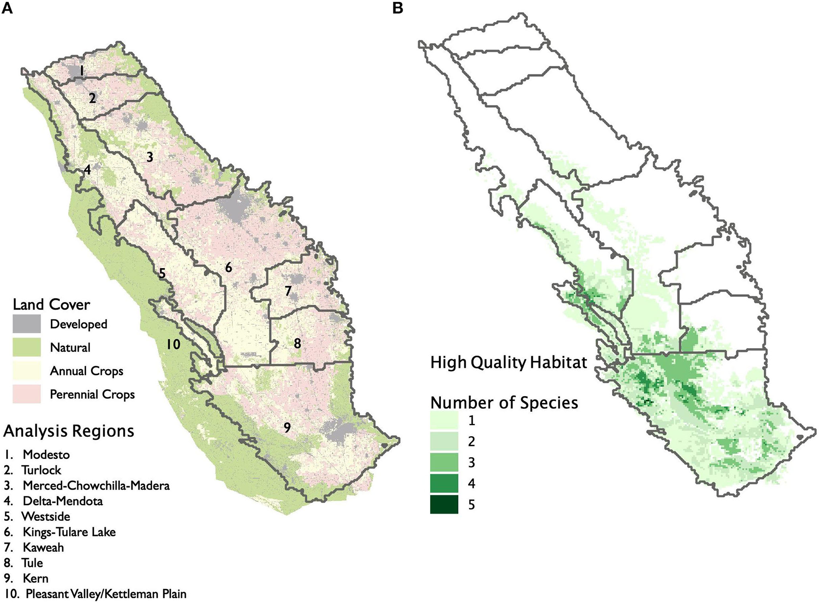
San Joaquin Valley Study Area. (A) The present day land uses, distinguishing remaining natural areas from annual and perennial crops, and including the Diablo and Temblor ranges to the west outside the valley floor. The 10 regions shown are analysis units for our study, which correspond to subbasins designated for coordinated groundwater management by the California Department of Water Resources (some regions group multiple subbasins into one unit for analysis purposes). (B) Aggregate potential habitat quality across the study area for five focal species (selected based on habitat needs deemed representative of the over 35 listed plant and animal species for the upland ecosystems in the San Joaquin Valley). Comparison of the natural area at right shows that most high quality areas serving several species have been converted to agriculture.
This economic success has imposed costs on wildlife, human health, and infrastructure. Agricultural expansion has been the primary cause of biodiversity loss in the SJV; today over 35 wildlife and plant species are listed as threatened or endangered and are now restricted to a relatively few remaining patches of suitable habitat with some species losing up to 98% of their habitat range (Williams et al., 1998; Stewart et al., 2019). Agriculture in this area has also contributed significantly to impaired air and water quality, leading to chronic human health problems (Meng et al., 2010; Lockhart et al., 2013; Almaraz et al., 2018). Groundwater extraction (Konikow, 2015) has resulted in large-scale land subsidence, with parts of the Valley sinking by over eight meters since the early 20th century, imperiling storage capacity and key portions of the surface water infrastructure on which the SJV depends (Faunt et al., 2016).
In response to these challenges, and amid significant drought-driven fallowing (Melton et al., 2015), California passed the Sustainable Groundwater Management Act (SGMA), which, among other requirements, obligates locally governed groundwater subbasins to develop plans that will achieve sustainable groundwater use over the next two decades (Leahy, 2016). Most of the subbasins in the San Joaquin Valley are categorized as critically overdrafted, suffering the worst effects of overdraft (CDWR, 2019). As a consequence many of these subbasins will face the most severe groundwater pumping restrictions that are currently being established by local governance processes, and which are to be phased in during a 20-years adaptation period. In the absence of basin-wide coordination and supply augmentation, prior research has estimated that complying with SGMA may require a reduction in average cultivated area exceeding 300,000 hectares (725,000–750,000 acres) over the next 20 years (Hanak et al., 2019)1.
1.2. Analytically Informed Multi-Benefit Planning Can Improve Adaptation to Scarcity
While it poses a great challenge, the impending transformation in the SJV also presents an opportunity to proactively shape the landscape in ways that not only ensure agricultural and water sustainability, but also to achieve many other socio-ecological goals, such as biodiversity protection and improved human health (Kelsey et al., 2018). However, given that achievement of many of these objectives is determined by where things happen on the landscape (rather than simply the aggregate amounts of cultivation, retirement, or restoration), stakeholders need a systematic way to integrate these objectives to inform multi-benefit spatial planning. Here we present a multi-part analytic approach that (1) develops estimates of business-as-usual responses to SGMA, (2) optimizes for habitat conditional on those uncertain BAU futures, and (3) assesses potential co-benefits (Figure 2 and section 2).
Figure 2
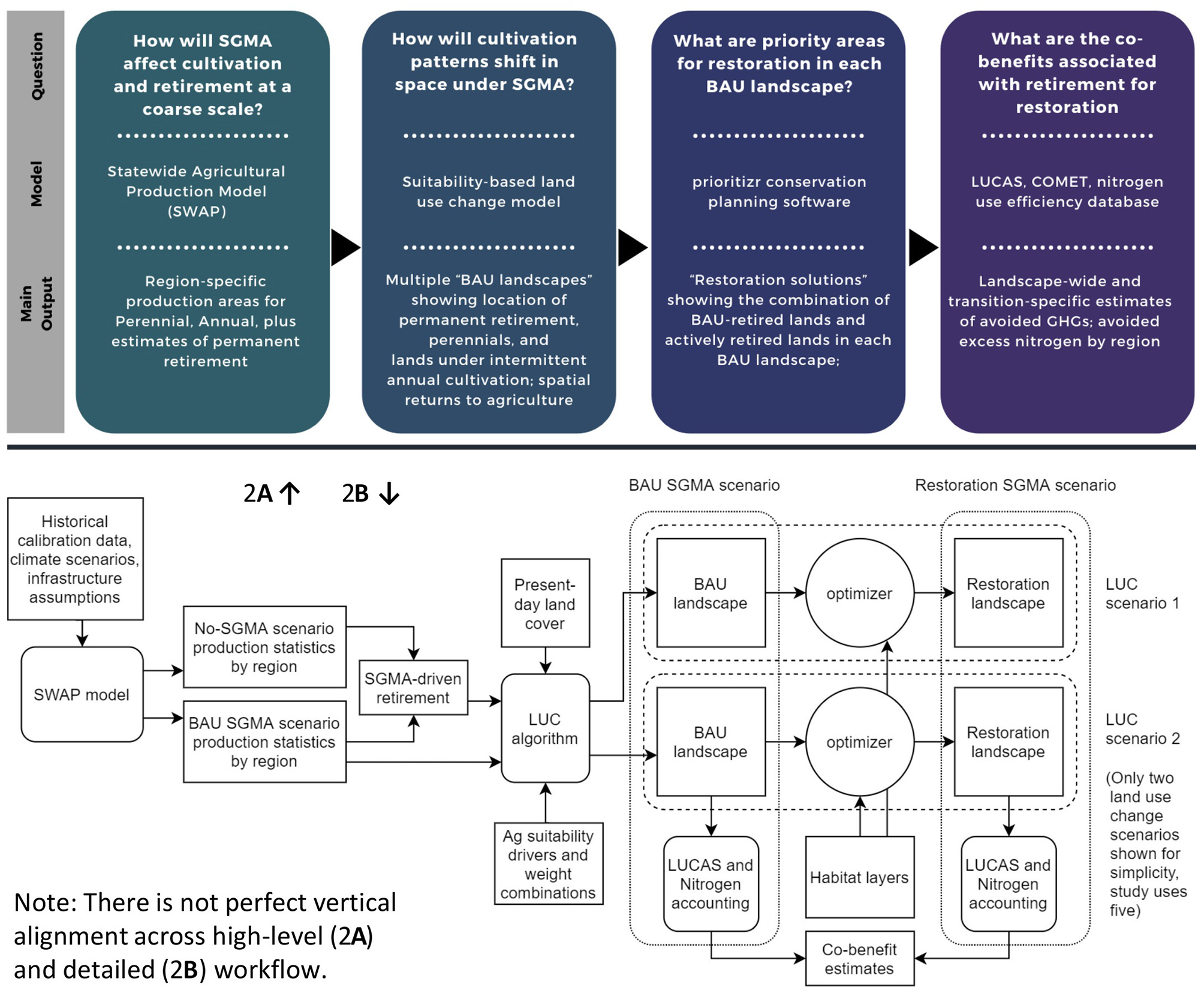
Overall modeling workflow, linking regional economic modeling, land use change, conservation planning, and co-benefits assessment. (A) (Upper) Shows the high-level workflow in terms of questions, models, and the form of output at each step. (B) (Lower) Shows the connections across workflow at a more mechanistic level, while highlighting the scenario logic. The paper focuses on characterizing BAU SGMA and Restoration SGMA scenarios, while recognizing uncertainty in their exact spatial patterns (LUC scenarios).
A key element of our approach is built around recognizing that multi-benefit planning in a stressed landscape requires first understanding how it may evolve in the absence of strategic shaping actions that consider non-market benefits. This evolution is of course uncertain, but multiple plausible BAU landscapes need to be considered in order to account for changing spatial patterns that govern the opportunity costs of habitat restoration, and the potential to shift cropping patterns to accommodate habitat and agriculture simultaneously. In recognition of this uncertainty, our analysis is explicitly organized to help inform engagement between conservation actors and agricultural land managers about how habitat goals can be achieved in ways that benefit communities in the SJV.
In some places, retirement under BAU conditions may align well with opportunities for habitat restoration. However, in other cases, collaboration would likely involve conservation or government actors providing compensation to achieve consolidated retirement of specific agricultural land for habitat—the goal being to direct inevitable land retirement to places where it can provide multiple benefits, while in turn avoiding retirement in areas that are less valuable outside of agricultural use. To help clarify the extent of coordination required, our summary results identify whether selected components of the solution are on land that would likely be retired under BAU conditions anyway (“BAU-retired”) or whether they would require active retirement and restoration in exchange for leaving other BAU-retired lands in production. Our results also allow comparison between the region-specific land requirements for habitat relative to SGMA-driven fallowing and permanent retirement, which in turn provides an indication of the potential for swapping infrequently cultivated areas and areas for restoration. Finally, we also estimated enhanced soil carbon sequestration and benefits in the form of reductions in nitrogen application associated with the transition from cultivation to restoration, which serve as examples of co-benefits that may be tied to incentive programs, provided appropriate additionality conditions are met.
The approach presented here integrates established methods in an innovative way that is useful for guiding on-the-ground action. Mathematically, our consideration of different land use change scenarios corresponds to considering multiple cost surfaces in systematic conservation planning, the importance of which has been examined previously (Carwardine et al., 2010), though does not appear to be routine. And while others have examined direct optimization of habitat-enhancing actions in landscapes under water stress (Bourque et al., 2019), or examined evolution of agricultural landscapes and their water use in the absence of constraints (Wilson et al., 2016), simultaneously incorporating fine-scale, resource-constrained, land use change modeling within the planning and optimization process is important and underutilized. The inclusion of resource constraints is necessary for realism, and while they are often incorporated in hydrologic or economic optimization models (Harou et al., 2009; Howitt et al., 2012), these models are typically specified at a policy-relevant regional scale that is too coarse for targeting restoration with spatially varying habitat potential. Combining these approaches represents an advance that can help create better outcomes in the SJV and be generalized to other stressed agricultural landscapes.
2. Materials and Methods
Below we briefly describe each step within Figure 2, with additional detail provided in the Supplementary Information. However, before delving into each of the modeling approaches, we lay out key aspects of the scenario terminology used and how they relate to each other.
2.1. Defining Multiple Scenario Dimensions for Future Landscapes
This study involves development of scenarios along multiple dimensions, with each dimension associated with a different modeling step. At the highest level, we consider futures with and without SGMA, which refer to annual average outcomes in the long-run after SGMA would be implemented (i.e., post-2040). We label a future with SGMA as “Business-as-Usual,” where the assumption is that SGMA will be implemented, but without specific concern for securing habitat2. The agricultural production and retirement statistics for the BAU scenario are generated at the coarse regional scale (i.e., the regions in Figure 1) by the SWAP model (see below), with retirement identified by comparing to a “No-SGMA” scenario also modeled in SWAP. This latter scenario is not our focus but rather is used instrumentally within the workflow to generate estimates of SGMA impacts. The last SGMA scenario is a “restoration scenario” which refers to what a post-SGMA future would look like if habitat considerations were proactively taken into account during SGMA implementation. These two scenarios are shown by the dotted vertical groupings in Figure 2B.
On a second scenario dimension, the “BAU” and “restoration” scenarios are made spatially explicit at the pixel level, and vary in their exact spatial configuration even as aggregate regional values are held constant. To indicate a spatial component to the scenario, we use the term “landscape.” BAU landscapes are created by spatializing the region-level production statistics from SWAP according to a land use change algorithm. Restoration landscapes are created by spatially optimizating for habitat taking into account features of the BAU landscapes. Therefore, an individual landscape is a combination of the “SGMA scenario” (BAU or restoration) and the “Land use change (LUC) scenario” —with individual LUC scenarios based on different assumptions about what drives agricultural suitability and retirement. More detail on each step is provided below.
2.2. Modeling Regional Impacts on Agricultural Production and Retirement
To generate plausible BAU landscapes, we first estimated changes in agricultural production necessary to meet groundwater sustainability targets within regions. We apply the long-established Statewide Agricultural Production Model (SWAP) with updated calibration methodology and data (Howitt et al., 2012; Mérel and Howitt, 2014), calibrated to SJV conditions and a representative 21-years historical hydrology (with adjustments for anticipated near-term climate change)3. The SWAP model simulates water supply availability and economic conditions that govern how agricultural producers are likely to respond to SGMA for 10 different regions of the SJV. Specifically, SWAP provides per-region estimates of average annual cultivated acreages under different water supply and policy scenarios, and intermediate outputs are used to infer the levels of permanent retirement necessary to achieve SGMA-compliant water use. SWAP also estimates revenue associated with each crop category, which is used to inform costs of securing land for habitat restoration in the optimization step described farther below.
2.3. Creating Spatially Explicit BAU Landscapes
To spatialize these changes within regions, we used a suitability-based heuristic land use change (LUC) algorithm (National Research Council, 2014) customized for this study. It begins with present day cropping patterns but updates them to align consistently with the region-specific production statistics output by SWAP in the step above. Recognizing that drivers of landscape change are uncertain, we developed multiple LUC scenarios based on different weighting combinations of four different potential drivers of agricultural suitability. These included high level assessments of “land assets,” “land quality” (both from Thompson and Pearce, 2018), as well as custom-developed groundwater availability and surface water availability layers (described in Supplementary Information). The algorithm operates such that the lowest ag suitability pixels in each region are most likely to be retired, and also that, in regions where particular classes (namely perennial) expand, expansion occurs on high quality land currently occupied by lower value annuals.
Each of the drivers that serve as input to create the ag suitability layer is a raster normalized so that a pixel value of 1 correlates with (all else equal) high suitability for agriculture, and zero indicates the lowest suitability. For example, because “land impairment” is assumed to be inversely correlated with agricultural suitability, the highest values in the original land impairment layer receive a zero, while the lowest values receive a 1. We consider five LUC scenarios in total: One for equal weighting of all four drivers, and one each where the majority weight (75%) is on each of the four specific drivers (with corresponding names based on the primary driver, as in Figures 5, 7). For example, the “Groundwater” LUC scenario has 75% weight on the groundwater suitability driver layer, and 8.33% weight on each of the other three drivers.
The result is a description, for each BAU landscape, of how much area in each pixel in the landscape is under perennial crops, under annual crops (as well as region-specific cropping intensities), and how much is retired. Different users may find different scenarios more or less plausible and the workflow allows for easily generating new scenarios based on alternate weightings. Additional data collection and expert input could further refine these scenarios, with region-specific differences in drivers or more data-driven approaches based on multinomial logit downscaling (Chakir, 2009). This step (and the subsequent spatial optimization step) are presented at 1,080 m resolution, which balances several considerations. While somewhat finer resolution would be possible (habitat and some other data are provided at 270 m), using 1,080 m pixels also serves to enforce a minimum area worth engaging in for conservation effort. It is also important to bear in mind that actual areas of different land categories are tracked within each pixel, so, while the pixels are coarse, our workflow does not assume that the entirety of the pixel is of one particular class. This aspect significantly mitigates potential error arising from coarse pixelization, while also increasing the speed and decreasing memory requirements for the land use change and optimization modeling.
2.4. Spatial Optimization to Generate Restoration Landscapes
The next major component of our analysis involves identifying priority areas for restoration when considering opportunity costs to agriculture, with a focus on locations that are consistent across multiple plausible future BAU landscapes (i.e., across multiple LUC scenarios). We utilized systematic conservation planning (spatial optimization) software to optimize the selection of lands for restoration (Beyer et al., 2016; Hanson, 2020), repeating the process for each BAU landscape and then examining areas of overlap, both across solutions, and with areas considered likely to be retired under business as usual. In addition to cost surfaces derived from the BAU landscapes, the key inputs are maps from (Stewart et al., 2019) indicating where restoring lands would result in high quality habitat for each of five target species: San Joaquin kit fox (Vulpes macrotis mutica), giant kangaroo rat (Dipodomys ingens), Tipton kangaroo rat (Dipodomys nitratoides nitratoides), blunt-nosed leopard lizard (Gambelia sila), and San Joaquin woolly-threads (Lembertia congdoni). These species collectively are believed to be representative of the habitat needs of the more than 35 listed plant and animal species that occupy the once abundant upland desert scrub and grassland habitats of the region (Williams et al., 1998; Germano et al., 2011; Stewart et al., 2019).
The optimization was implemented as a cost-minimization problem in which the agricultural opportunity cost layer was treated as the cost layer (with a boundary penalty, discussed below), and the constraints to be achieved were minimum areas of high quality habitat. More specifically, we required the optimizer to find restoration solutions that secured an additional 25,000 acres (10,117 ha) of high quality habitat for each of the species, i.e., restoration of a specific area could count toward the target of multiple species at once, but securing extra habitat for one species could not come at the expense of habitat area for another species falling below the minimum area threshold. Here, high quality habitat was taken as the top decile of the continuous distribution of habitat quality for each species from Stewart et al. (2019). These targets are ambitious, but are generally consistent with existing targets for population recovery specified by the U.S. Fish and Wildlife Service, though those goals did not consider retirement and restoration of agricultural land (Williams et al., 1998). The large targets also ensure a broader palette that recognizes not all priority land will be restored. We also included a “boundary penalty” which penalizes overall edge-length of natural lands under the final post-restoration configuration, so that solutions which create clusters of aggregated habitat (whether existing natural or newly restored) are preferred over highly pixelized solutions. A more extensive enumeration of assumptions and constraints underlying the optimization framework, as well as sensitivity assessment, is provided in the Supplementary Information.
2.5. Co-benefits Assessment
We estimate changes in average annual excess nitrogen applied by assembling crop-specific application rates and nitrogen use efficiencies (NUE) relevant for SJV crops. The values assigned to annual and perennial cropland in each region are area-weighted by the 18 SWAP crop categories for each region, drawing on multiple sources for application rates and efficiencies (see “Excess Nitrogen Application” portion of Supplementary Information). This provides differentiation of average NUE and excess N applied by each region's crop composition and cropping intensity. Existing groundwater nitrate levels were estimated for each SWAP region using estimates from the State Water Resources Control Board's Groundwater Ambient Monitoring and Assessment Program. We also include a coarse estimate of avoided N emissions derived from COMET-Farm runs that were generated for use in California-tailored implementation of COMET-Planner (Swan et al., 2015, 2018)4.
Finally, we utilize and spatially propagate a single-cell version of the land use and carbon scenario simulator (LUCAS) model developed for California (Sleeter et al., 2019), which was designed to estimate the impact of land-use change on ecosystem carbon balance. Net sequestration of soil carbon is tracked for all relevant transitions (perennial to retired, annual to restored, etc.—see Supplementary Information for complete list) until a time horizon of 2100. We then spatialize the single-cell transitions under the BAU and restoration land use scenarios by comparing to the present day land cover, and examine the cumulative difference between the BAU and restoration scenarios in 2100. Unlike other aspects of this modeling workflow, the GHG assessment assumes generic “annual” and “perennial” crop types, rather than estimating those two categories as weighted combinations of region-specific cropping patterns. It does, however, approximate the cropping intensity of annuals within different regions. Lastly, because there is uncertainty in what the most appropriate restoration end-state may be at different sites, and also what the fate of retired lands will be, we run the model for different restoration end states and different retirement end states, to assess sensitivity. Restoration end states are parameterized as grassland or as shrubland, and retired end states are modeled as “abandoned” or as “abandoned with discing,” a process where farmers lightly plow to prevent undesirable flora and fauna from establishing long-term.
3. Results
3.1. Aggregate Land Use Varies Significantly by Region, With a Mix of Permanent Retirement and Temporary Fallowing
We estimated that ~86,000 hectares of existing irrigated cropland will be permanently retired by 2040 as part of economically optimal strategies to achieve the groundwater sustainability requirements of SGMA (Table SR1, total of black “Retired” area in Figure 3). These results rely on anticipated surface water supplies under a projected future climate in 2030 derived from the CalSim Water Model and local surface water supply data. They also assume that no supplemental water supplies are developed and delivered to these basins, but do assume that the regions maximize their existing capacity for groundwater recharge during wet years (Table SM1).
Figure 3
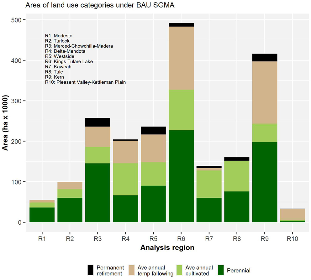
Projected distribution of land uses on present day agricultural footprint for each region in our study area under a BAU SGMA future. Black corresponds to permanent retirement relative to a no-SGMA future, while the combination of average temporary fallowing and average cultivation of annuals represents a footprint of land under annuals under BAU SGMA. Annual croplands are generally lower return and more flexibly re-allocated than land under perennial crops (dark green).
This retirement total represents 4% of the currently cultivated landscape overall, though the proportion varies from 0 to 8% across regions, based on relative surface water supplies, dependence on groundwater, as well as applied water demands of crops. In addition, over a representative 21 years of hydrology, a substantial area (totaling ~540,000 ha/year on average, or 27% of all non-retired ag land) is expected to be intermittently fallowed in our modeled BAU scenario. Comparing with the current agricultural footprint indicates that much of this fallowing would happen even in the absence of SGMA, due to natural and policy-driven variability in water available for agriculture, but we find SGMA to be responsible for a reduction of annual average cultivated area of ~160,000 ha (Table SR1). This varies across regions as well, with, for example, the Tule region (R8) seeing negligible annual fallowing, but 8,500 ha of permanent retirement, while projections show the Pleasant Valley/Kettleman Plain region (R10) experiencing negligible permanent retirement but a very low average annual cultivation relative to the area retained within the agricultural footprint.
3.2. Spatial Patterns of Retirement Vary by LUC Scenario, but Reveal Consistent Hotspots
Considering five scenarios that reflect the uncertainties in how land quality and water availability will drive the location of retirement, there are strongly consistent patterns, with many areas predicted to be retired under most or all of the scenarios (Figure 4). Areas of concentrated retirement occur in the north-central Kern region (R9), in the southwestern corner of the Tule region (R8), along the eastern edge of the Westside region (R5) and western edge of the Kings-Tulare Lake region (R6). More variation exists within the northern regions, including Modesto (R1), Turlock (R2), Merced-Chowchilla-Madera (R3), and Delta-Mendota (R4). Greater variation within the northern regions reflects lower correlation between drivers of retirement. Some boundary effects emerge based on the assumption that analysis regions will engage in no groundwater trading across regional boundaries, which is consistent with the current political context but may change during the 20 years leading up to SGMA compliance. To the extent this assumption is relaxed, some stark boundaries may be less pronounced, with more retirement diffusing across regional borders.
Figure 4
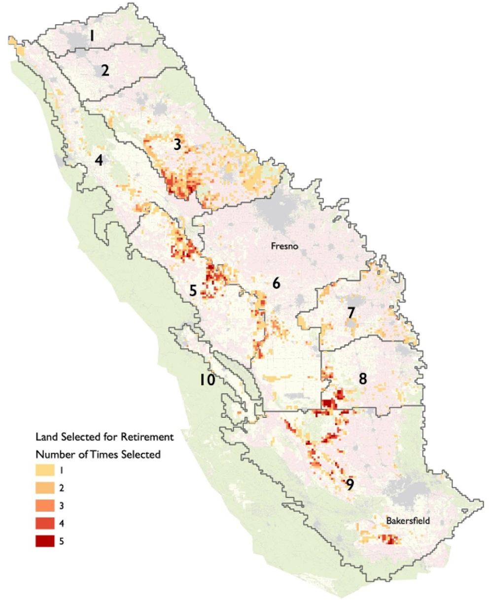
Number of times each pixel was selected for retirement under BAU SGMA across the five LUC scenarios. The figure highlights several “hotspot” clusters where retirement is likely regardless of the key determinants of suitability. Note that the total area identified as retired under each scenario is smaller than the visual footprint of heatmap pixels. This is due to (1) imperfect overlap of all five scenarios, and (2) pixels are counted as retired if any agricultural land existing within the pixel was retired, which could only be a fraction of the total pixel area (the fraction of the pixel retired is tracked throughout our analysis chain).
3.3. Spatial Optimization Reveals Consistent Priority Restoration Areas
The total area selected for restoration across the different solutions was consistent across LUC scenarios, ranging from 18,700 to 19,100 hectares (Figure 5, Table SR2). This is only 37–38% of what would be required to reach restoration targets if high quality habitat did not overlap among the target species, which reflects efficiency gained by the optimizer identifying parcels that serve multiple species.
Figure 5
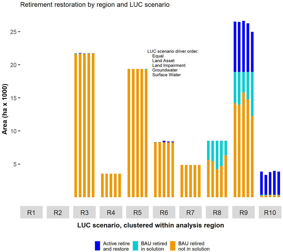
Retirement and restoration by class, region, and LUC spatial scenario. “BAU retired in solution” refers to land identified for restoration that is projected to be retired even in the absence of strategic coordination. “Active Retire and Restore” refers to land identified for restoration that would otherwise remain in production under the BAU scenario, and would require active coordination to bring under restoration—possibly by working to prevent retirement of lower habitat value parcels “in exchange” for accepting the retirement of the high-priority parcel. “BAU retired, not in solution” is land that is projected to be retired and not targeted for restoration. Each region contains five bars corresponding to each land use change scenario, in the order overlayed on the plot (no retirement or restoration is predicted or selected in R1 and R2). Overall, the magnitude and relative proportion of each land use type are generally consistent across scenarios, with modest sensitivity to the amount and distribution of BAU-retired land in the solution across R8 and R9.
Across all scenarios, priority restoration areas were concentrated in the southern part of the SJV (Figure 6). Overall, the results indicate that restoration solutions consistently identify several contiguous clusters for restoration, in addition to other areas that are more scenario-dependent. Restoration was concentrated in four core areas: around Pixley National Wildlife Refuge in the southwestern portion of the Tule region (R8), around Kern National Wildlife Refuge in the north-central part of the Kern region (R9), in the western Kern region, and the northern portion of the Pleasant Valley/Kettleman Plain (R10) region. These clusters occur where BAU scenarios consistently indicate lower return agricultural land (retired, or routinely fallowed) intersecting with areas that could serve multiple species and provide connectivity to existing natural lands, if they are restored. Out of the eight regions where retirement was predicted to occur, only four regions featured in restoration solutions, with amounts of BAU-retired land selected for restoration ranging from <1% in the Merced-Chowchilla-Madera region (R3) to between 26 and 50% in Tule (R8), depending on LUC scenario. Only three regions (8–10) had substantial areas selected for restoration overall, with Kern (R9) representing the vast majority of restoration at between 10,800 and 12,700 ha, or 58–68% of the total (Figure 5).
Figure 6
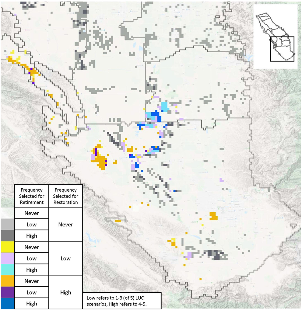
Areas selected for restoration in order to create 10,117 ha (25,000 acres) of new high quality habitat for each of five focal species while minimizing additional cost to the agricultural economy. Colors simultaneously reflect the relative frequency with which lands were selected to be a part of the habitat solution, as well as the frequency lands were identified as likely to be retired. Together these provide an indication of where retirement and restoration are well-aligned (blue colors), and where shifting production may be useful to enhance restoration while preserving production.
The restoration solutions varied significantly by region in terms of the extent to which BAU-retired land was selected for restoration. They also varied in terms of how much prioritizing of active restoration (in areas not retired under BAU) would optimally be used to achieve habitat goals (Light blue vs. dark blue in Figure 5). The importance we placed on avoiding fragmentation (considering newly restored or existing natural land together), and the optimizer's attempt to capitalize on sites that serve multiple species resulted in solutions that identify 9,700–11,400 hectares for retirement and restoration that are not otherwise expected to be retired under BAU scenarios (“Active Retirement and Restoration” in Figure 5 and “Unretired-Low” or “Unretired-High” in Figure 6, see also Table SR2). This is despite there being significant areas of unselected retired land, which is generally lower cost to secure for habitat. However, the existence of unutilized BAU-retired land (“BAU retired not in solution”) suggests opportunities for proactive engagement to shift cultivation to less valuable habitat areas, rather than securing retirement above and beyond that imposed by SGMA (see section 4).
3.4. Soil Carbon Sequestration and Mitigation of Excess Applied Nitrogen Are Modest at a Statewide Scale, but Can Be Significant Locally
In a no-SGMA future, our modeling results indicate an average of ~199,600 tons of excess nitrogen (nitrogen applied but not consumed by crops) would be applied annually across our study area. The retirement and temporary fallowing associated with SGMA is predicted to reduce this amount by ~18,800 tons annually, or 9%. This incremental change due to SGMA-driven retirement is modest, but given nitrate and air pollution issues in the SJV (Lockhart et al., 2013; Almaraz et al., 2018), it may still have noticeable local effects, depending on exposure pathways. Our results also show limited correlation between “retire and restore” areas with areas having high existing nitrate concentrations in groundwater. The incremental displacement of applied nitrogen associated with targeting for restoration is also small, 252–307 tons annually, or just a fraction of a percent of valley-wide excess N (Table SR3). This suggests that if concern over nitrate contamination is a priority, it must be actively considered in the optimization, rather than treated as a co-benefit.
Figure 7 shows the cumulative soil carbon sequestration impact of restoration scenarios assuming an evenly phased transition from 2021 to 2040. These are based on propagating the dynamics shown in Figure SR1 to represent the phased implementation, and to account for the fact that across different LUC scenarios, restoration portfolios may involve different areas transitioning from specific crop classes to retired or restored. For example, one LUC scenario may involve more transition of perennials to restoration, while another may involve more transition of annuals, while another may prioritize more land that would have been retired anyway. Overall, restoration would lead to a net enhancement of soil carbon that would average 1,590,000 tCO2e for restoration to Grassland and 1,180,000 tCO2e for restoration to Shrubland, when averaged across parametric uncertainties shown more explicitly in Figure 7. Parametric uncertainty is significant, but in all of the forty combinations of parameters and spatial scenarios, the impact of a strategic retirement and restoration strategy is positive, with the cumulative per-hectare net increase in soil carbon through 2100 ranging from 27 to 133 tCO2e (7–36 tons of actual carbon). Importantly, the primary drivers of variation are either decision variables or are measurable in advance of implementation: Variation is driven first and foremost by initial soil carbon (as indicated by the gap between filled and unfilled points having the same shape and color). The next most important factor is whether restoration is to grassland or shrubland, as indicated by the gap between colors for the same shape and fill. Least important are the impact of discing in retirement and variation across spatial scenarios. In the absence of other land use pressures, it is unlikely that a majority of land would be disced over an 80-years time horizon, but other end uses of abandoned land may involve soil disturbance or complete loss of vegetation as well, in which case discing can be viewed as a coarse proxy for these other disturbances.
Figure 7
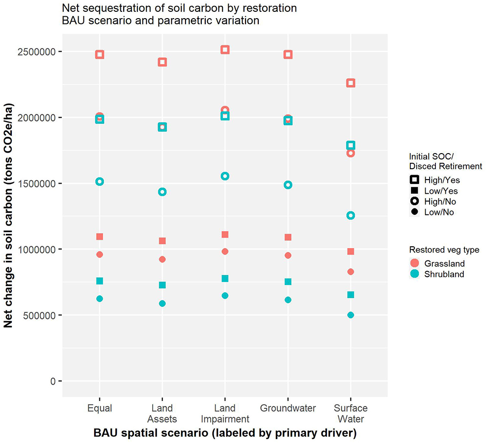
Positive impact of restoration on soil carbon through 2100, reported as CO2e for comparison to social costs and other GHG sources. The results assume that 5% of the lands identified for restoration are restored each year from 2021 to 2040, but present cumulative totals as of the year 2100. Initial SOC refers to whether the soil carbon in 2020 was assumed to be a high value (100 t/ha) or low (40 t/ha). Disced retirement refers to whether retired land is routinely disturbed to prevent weed growth that could contaminate nearby cultivated fields.
Because soil carbon represents only part of the overall GHG impacts associated with agriculture, we also analyzed a fine-scale model-generated dataset of output from the COMET-Farm modeling tool, which speaks to nitrous oxide emissions. When filtered based on geography representative of the SJV, the dataset indicated an average annual avoidance of 0.43 tCO2e ha/yr in N2O emissions over the first 10 years following conversion of annuals to grasslands. While the sampling is not precisely statistically representative of the restored area, over 80% of points modeled in COMET-Farm fall between 0.08 and 0.84 tCO2e ha/yr, with a median value of 0.32, suggesting that a 10 years N2O-derived emissions reduction of several tons CO2e is robust, significantly enhancing the GHG benefits of strategic retirement and restoration beyond that of soil carbon alone.
4. Discussion
Our region-level results demonstrate that reductions in average irrigated cultivation necessary to achieve sustainable groundwater use in the SJV will be significant, likely being met via a combination of permanent retirement and temporary fallowing. Notably, however, the permanent retirement required is a relatively small fraction of the agricultural footprint (~4%), and the total reduction in average annual cultivated area attributable to SGMA is also less than some previous studies (Hanak et al., 2017, 2019). While partitioning all the sources of the difference between this and previous studies is not feasible here, one major driver is likely to be an improved calibration technique that better represents farmer adaptation to intermittently scarce water supplies. Our spatial results demonstrate that while the location of some permanent retirement depends on which factors turn out to be the most influential in driving land use changes, there are hotspot clusters that are consistent over multiple assumptions about drivers of land use. Similarly, several areas are robustly identified as priorities for restoration, using a mix of BAU-retired land and actively retired land. Consideration of these anticipated retirement patterns will play an important role in designing the least disruptive and most cost-effective strategies for restoring high quality habitat for target species and achieving other co-benefits. However, achieving positive outcomes will depend on careful coordination and implementation, including decisions about geographic scope and constraints on water trading. We next discuss the benefits that can be achieved by successfully negotiating these challenges, and then elaborate on the policy and implementation considerations needed to address them.
4.1. Multi-Benefit Planning for Restoration Holds Significant Potential for Expanding and Consolidating Habitat, but Realistic Recovery Goals and Coordinated Protection of Natural Lands Are Key
Our results show that it would be possible to achieve ambitious habitat restoration targets (~19,000 ha that ensures at least 10,000 ha of high quality habitat for each focal species) within a small number of new or expanded protected areas. These consolidated natural and restored areas would serve a suite of listed species on only 1% of the land currently allocated to irrigated agriculture, using only about 20% of the land area expected to be retired to achieve groundwater sustainability. Although not explicitly considered in the Recovery Plan for Upland Species of the San Joaquin Valley (Williams et al., 1998), the large-scale creation of new or expanded protected areas through the use of otherwise retired farmlands has the potential to achieve species recovery (Stewart et al., 2019), though success is by no means guaranteed, particularly if restoring isolated islands of farmland (Lortie et al., 2018). However, a focus on creating new restored areas contiguous with natural areas occupied by the target species has better prospects for success. This is especially true when restoring or connecting to habitat already containing species that provide foundational (e.g., shrubs; Lortie et al., 2018, 2020; Westphal et al., 2018) or keystone (e.g., kangaroo rats; Prugh and Brashares, 2012) species, as these are known to facilitate enhanced habitat values and encourage additional plant and animal species occupancy. This strategy would allow species to naturally migrate to restored lands, avoiding active reintroduction efforts, which can be costly, hard to permit, and often have low success rates.
While the focus of this analysis is on identifying priority lower-return agricultural lands for strategic restoration, the protection and proper management of existing natural habitats across the western SJV will also be essential for species recovery. The importance of natural lands to the long-term persistence of SJV endemic species has been confirmed in recent rangewide genetic studies on the endangered blunt-nosed leopard lizard (Richmond et al., 2017) and giant kangaroo rat (Statham et al., 2019). Intact and protected natural lands will likely become increasingly important to species recovery as the climate changes and brings warmer and drier weather to large portions of the SJV (Westphal et al., 2016; Stewart et al., 2019). Importantly, the fact that a significant fraction of retired lands were not selected as high priority in our optimizations does not necessarily mean they lack potential for enhancing biodiversity in the SJV. Conservation actors should still maintain awareness of low-cost opportunities for restoration outside our priority areas, provided they have confidence in their habitat benefits.
4.2. Land Use Change Modeling and Optimization Clarify the Opportunity Space Between Shifting Cultivation and Additional Retirement, Each With Varying Co-benefits
Importantly, our analysis does not recommend a specific landscape based on the optimizer results. Rather, the robust clusters of areas selected for restoration identify a palette within which contiguous natural landscapes can be created, using a mix of BAU-retired land and active retirement and restoration. While it is expected that successful restoration would involve securing a significant fraction of the priority areas, the results do not constitute a fully prescriptive landscape planning design and, crucially, do not specify what should happen on other retired or frequently fallowed lands. In particular, when active retirement is undertaken in priority habitat areas, the retirement involved will often free up water rights that could then be put to several different uses, each of which varies in how benefits are distributed between conservation goals, landowners, and the broader agricultural community. We would expect that in most areas, many stakeholders will place a high priority to keep as much land in production as possible, which can be achieved by redistributing water rights associated with lands prioritized for active retirement and restoration. This redistribution could result in avoiding retirement of land that would otherwise be retired, or more intensively cultivating land that would have been more frequently fallowed. Alternatively, with sufficient compensation, farmers may prefer the additional reduction in footprint due to inefficiencies at low cropping intensities (e.g., discing during fallow periods). In other cases, alternative land uses, like installation of low impact solar energy facilities, will be a viable option that can compensate landowners for lost agricultural income (Wu et al., 2019).
In cases where retirement occurs to achieve habitat objectives, the avoidance of externalities created by intensive agriculture may be non-trivial. For example, improving groundwater quality is an urgent priority in many parts of the SJV (Moore and Matalon, 2011; Hanak et al., 2019). Application of nitrogen-based fertilizers is the major contributor to nitrate contamination of groundwater with significant consequences for human health through multiple channels (Keeler et al., 2016), that have impacted numerous communities in the SJV who depend on shallow groundwater wells for drinking water (Lockhart et al., 2013). Our estimates of reductions in application of excess nitrogen across the study area are substantial and may have meaningful benefits for communities, which would be incrementally improved by retirement. While mechanisms connecting fertilizer application to exposure are complex (Keeler et al., 2016), reduced N application may come with air quality benefits as well, via reduction in N2O and particulate matter exposure from agriculture (Almaraz et al., 2018).
However, there were no strong correlations between areas selected for active retirement and restoration (which would have an associated reduction in N application) and regions where higher nitrate contamination exist. For example, in our study area, the Kaweah Region (R7) has well-documented high levels of nitrate contaminated groundwater; however, no restoration was targeted in that region based on habitat values alone. In contrast, very large areas were targeted for restoration in Kern (R9), where nitrate contamination is moderate (Table SR3). This is not surprising given that selecting areas for their potential water quality benefits was not part of the optimization. Given the importance of this issue in the region and the potential to take advantage of incentives and funding streams tied to different benefits like improved water quality, planning could be enhanced by incorporating potential for water quality benefits (or other outcomes) as part of the spatial planning for retirement and restoration. By spatially prioritizing restoration in areas where potential habitat quality is high and in close proximity to people (particularly disadvantaged communities who have been the most impacted by impaired water quality), it could be possible to simultaneously achieve groundwater sustainability, support species recovery and improve human well-being.
Finally, protection and restoration of natural habitats can also play a role in building soil carbon and mitigating climate change, a global issue. California has set and surpassed a goal to reduce GHG emissions to 1990 levels by 2020 (15% below a BAU scenario), with the additional goals to achieve emissions that are 40% below 1990 levels by 2030 (Office of the Governor, 2015) and 80% below 1990 levels by 2050. Cameron et al. (2017) have shown that land use management can play a significant role in helping California achieve its emissions reductions goals. Our study provides a specific path to a regional landscape approach to GHG reduction: The ~500,000–2,500,000 tCO2e of net soil carbon sequestration correspond to a small fraction of the state's overall goals of 172 MMT by 2030 and 345 MMT by 2050, though also requires a miniscule portion of land resources: The area restored also corresponds to <120th of 1% of the state's land surface area. And while this number is estimated for a longer time horizon, it also focuses only on soil carbon sequestration, rather than a full life cycle analysis (Kendall et al., 2015). Conservation and agricultural stakeholders may therefore wish to pursue cap and trade funding to achieve restoration goals given the large investments being made through California's carbon cap and trade program (Megerian, 2017; Taylor, 2017) given the contribution restoration of retired lands could make toward the state's goals while simultaneously achieving other benefits.
The quantitative co-benefits above are reported for the hypothetical (and undesirable) case in which all restoration on actively retired lands is met through net additional retirement, i.e., there is no shifting of saved water to maintain cultivation in other areas. This represents an extreme limiting case, both in terms of the likelihood that it would emerge as a preferred outcome by stakeholders across the regions, and because it does not account for the fact that some production will inevitably shift to other regions within or outside of the SJV. This does not mean that these co-benefits lose their importance, but rather that compensation for co-benefits and negotiation needs to account for coordinated shifts within regions, as well as leakage outside the region.
4.3. The Ability to Successfully Negotiate Beneficial Landscapes Requires Coordination and Enabling Policies
Despite the opportunity SGMA-driven land use change presents for constructive engagement between the conservation and agricultural communities, there are significant challenges to realizing multi-benefit outcomes while mitigating any negative impacts to those living and working in the SJV. Consolidating some of the agricultural land predicted for retirement into specific, relatively large areas where the greatest habitat benefits can be created will require strategic planning that can only be achieved through direct coordination and cooperation among water management agencies; each of which will have individual mandates and mechanisms for reaching groundwater sustainability. This level of planning and cooperation will be even more fundamental given the need and opportunity for simultaneously changing land use to achieve multiple benefits that include other habitat types (e.g., temporary wetlands that provide groundwater recharge) and renewable energy development (Bourque et al., 2019; Hanak et al., 2019). Consolidated and focused retirement and restoration will not only require flexibility in trading and transfer of water across boundaries, it will also require targeted incentives and policies that facilitate this kind of flexibility and that defray some of the costs associated with creating broader societal benefits (Jack et al., 2008).
One key area for coordination outside of the water realm is solar expansion. The potential for expanding solar in the SJV is gaining prominence, both as an offset to livelihood challenges, and in recognition of the need for proactive consideration to preserve high quality habitat and high quality agricultural land (Pearce et al., 2016; Wu et al., 2019). Our analysis does not consider competing pressure on lands from solar expansion, either in terms of disturbing existing natural land, or expanding into the current agricultural footprint—nor, crucially, as an opportunity to contribute to funding strategic land restoration. On the one hand, uncoordinated expansion of solar may increase the opportunity cost of securing certain lands for restoration, though we expect this effect to be small, as the majority of BAU-retired lands are not high priority for restoration, leaving large aggregates of BAU-retired land available for solar. On the other hand, and more constructively, demand for solar may actually present an opportunity for additional coordination to secure habitat. Environmental organizations could work with managers of larger landholdings on the margin of profitability (or under threat of retirement from poor water access) to blend installation of solar, habitat, and scaled-back ag operations. Future analytic work could also incorporate these considerations without fundamental changes to the workflow used here.
4.4. The Analytic Framework Presented Here Is Modular and Amenable to Additional Uncertainty Exploration
The impact of solar is just one among many uncertainties that may affect costs and opportunities for multi-benefit restoration planning. Considering a wide array of uncertainties and objectives will be an important element in developing a robust restoration strategy. While the results presented here focus primarily on uncertainty in BAU scenarios, supplemental work explored other issues including definitions of natural land, definitions of high quality habitat, variable importance of clustering, and alternate habitat targets. While our overall results are generally robust to the exploration of many of these assumptions (Table SR4), some issues were infeasible to explore within the scope of this paper (discussed with respect to each modeling step in the Supplementary Information). However, the workflow presented here is amenable to refinement of individual components and assessment of sensitivity to those refinements. High priority issues for such refinement and sensitivity assessment include alternate land use pressures and constraints, and more refined assessment of the opportunity costs as perceived by the agricultural community. Both of these could be achieved by a combination of stakeholder engagement, elicitation of expert knowledge, or additional empirical work to constrain predictions of fine-scale BAU land use change consistent with the regional predictions from SWAP (cf. Chakir, 2009). Long-term, it will also be important to incorporate additional spatially dependent objectives, such as siting for solar (Pearce et al., 2016) and managed aquifer recharge (Hanak et al., 2018), additional habitat or ecosystem targets, and the impact of climate on spatial patterns of suitability for all objectives considered.
5. Conclusion
Stressed agricultural landscapes exist in many areas around the globe and are experiencing significant shifts in land use. Aiding their transition to long-term sustainability is a key component of meeting food systems challenges in the 21st century. Facilitating their transition to more diverse agricultural landscapes featuring restoration of natural lands presents an unprecedented opportunity to reverse the impacts of natural habitat loss on the environment and people (Isbell et al., 2019). We show that proactive consideration of how these stressed landscapes will evolve can create an opportunity for strategic engagement, and demonstrate how that engagement can be guided by a spatial analytic and optimization framework. In the San Joaquin Valley specifically, we find that combining economic modeling and optimization illuminates opportunities for restoring land likely to be retired anyway, along with locations where strategic engagement can shape retirement patterns to benefit habitat and compensate farmers. Importantly, each element of the approach we illustrate here can be refined in a modular fashion based on stakeholder priorities, and the entire workflow can be reproduced in landscapes with varying degrees of data availability.
Statements
Data availability statement
R code and harmonized spatial data used to generate spatial land use change, spatial optimization, nitrogen co-benefit, and carbon co-benefit propagation are included at the following Open Science Framework archive: https://osf.io/gjtuw/. As described in the Supplementary Information, the SWAP, COMET, and California LUCAS models are published and institutionally maintained models. Readers are referred to published studies (cited within) and additional details are available upon request.
Author contributions
BB and TRK coordinated the design of the research and writing of the manuscript, with contributions from AV, SW, HSB, and PS. DM coordinated and implemented the SWAP agricultural economic modeling. AV and SW developed the approaches and data inputs for nitrogen, water suitability, and water vulnerability. TRK and HSB developed the habitat goals. BB designed and carried out the land use change modeling, spatial optimization, and co-benefits propagation. PS designed and implemented LUCAS simulation models of land state transitions and ecosystem carbon balance. TRK, TB, and BB developed the maps and figures. All authors contributed review and edits to the manuscript.
Acknowledgments
We would especially like to thank Jeffrey Hanson for responsive assistance with implementing the prioritizr package, Abigail Hart for valuable insights and reviews over the course of the project, and Amy Swan for continued engagement on the use of COMET outputs. This work also benefited from helpful input from Chris Anderson, Tim Bean, Rebecca Chaplin-Kramer, Dave Marvin, Ted Grantham, Stephen Hatchett, Peter Hawthorne, Richard Howitt, Dave Marvin, Keith Paustian, and Joseph Stewart and research assistance from Erin Pang. Any use of trade, firm, or product names is for descriptive purposes only and does not imply endorsement by the U.S. Government.
Conflict of interest
The authors declare that the research was conducted in the absence of any commercial or financial relationships that could be construed as a potential conflict of interest.
Supplementary material
The Supplementary Material for this article can be found online at: https://www.frontiersin.org/articles/10.3389/fsufs.2020.00138/full#supplementary-material
Footnotes
1.^ In this study, we refine this estimate with updated modeling and data, and also distinguish temporary fallowing from likely permanent retirement, finding significantly lower impacts, though direct comparisons of statistics associated with the SJV are further complicated by imperfect overlap of in the study areas.
2.^ We recognize it may be unusual to include a relatively new water sustainability policy as part of business-as-usual —which often connotes lack of responsive policy—but the focus of our paper is on the marginal effect of considering restoration assuming SGMA is implemented.
3.^ Calibration was conducted using actual historical water supply estimates from the period 1974–94, but the No-SGMA and BAU SGMA futures reflect adjustments to the hydrology that factor in 2030 climate using techniques developed for the California Water Commission.
4.^ COMET is a legacy acronym that originally stood for CarbOn Management and Evaluation Tool.
References
1
Almaraz M. Bai E. Wang C. Trousdell J. Conley S. Faloona I. et al . (2018). Agriculture is a major source of NOx pollution in California. Sci. Adv. 4:eaao3477. 10.1126/sciadv.aao3477
2
Beyer H. L. Dujardin Y. Watts M. E. Possingham H. P. (2016). Solving conservation planning problems with integer linear programming. Ecol. Modell. 328, 14–22. 10.1016/j.ecolmodel.2016.02.005
3
Bourque K. Schiller A. Loyola Angosto C. McPhail L. Bagnasco W. Ayres A. et al . (2019). Balancing agricultural production, groundwater management, and biodiversity goals: a multi-benefit optimization model of agriculture in Kern County, California. Sci. Total Environ. 670, 865–875. 10.1016/j.scitotenv.2019.03.197
4
California Department of Food and Agriculture (2018). California Agricultural Statistics Review 2017–2018. Technical report, California Department of Food and Agriculture.
5
Cameron D. R. Marvin D. C. Remucal J. M. Passero M. C. (2017). Ecosystem management and land conservation can substantially contribute to california's climate mitigation goals. Proc. Natl. Acad. Sci. U.S.A. 114, 12833–12838. 10.1073/pnas.1707811114
6
Cannon Leahy T. (2016). Desperate times call for sensible measures: the making of the California sustainable groundwater management act. Golden Gate Univ. Envtl. L. J. 9.
7
Cardinale B. J. Duffy J. E. Gonzalez A. Hooper D. U. Perrings C. Venail P. et al . (2012). Biodiversity loss and its impact on humanity. Nature486, 59–67. 10.1038/nature11148
8
Carwardine J. Wilson K. A. Hajkowicz S. A. Smith R. J. Klein C. J. Watts M. et al . (2010). Conservation planning when costs are uncertain. Conserv. Biol. 24, 1529–1537. 10.1111/j.1523-1739.2010.01535.x
9
CDWR (2019). Bulletin 118 Groundwater Basins Subject to Critical Conditions of Overdraft–Update Based on 2018 Final Basin Boundary Modifications. Sacramento, CA: CDWR.
10
Chakir R. (2009). Spatial downscaling of agricultural land-use data: an econometric approach using cross entropy. Land Econ. 85, 238–251. 10.3368/le.85.2.238
11
Chartres C. J. Noble A. (2015). Sustainable intensification: overcoming land and water constraints on food production. Food Security7, 235–245. 10.1007/s12571-015-0425-1
12
Damania R. Desbureaux S. Hyland M. Islam A. Moore S. Rodella A.-S. et al . (2017). Uncharted Waters: The New Economics of Water Scarcity and Variability. Washington, DC: World Bank.
13
Elliott J. Deryng D. Müller C. Frieler K. Konzmann M. Gerten D. et al . (2014). Constraints and potentials of future irrigation water availability on agricultural production under climate change. Proc. Natl. Acad. Sci. U.S.A. 111, 3239–3244. 10.1073/pnas.1222474110
14
FAO AQUASTAT (2018). Facts and Figures on Irrigated Areas, Irrigated Crops, and Environment. Rome: FAO AQUASTAT.
15
Faunt C. C. Sneed M. Traum J. Brandt J. T. (2016). Water availability and land subsidence in the Central Valley, California, USA. Hydrogeol. J. 24, 675–684. 10.1007/s10040-015-1339-x
16
Foley J. A. DeFries R. Asner G. P. Barford C. Bonan G. Carpenter S. R. et al . (2005). Global consequences of land use. Science309, 570–574. 10.1126/science.1111772
17
Germano D. J. Rathbun G. B. Saslaw L. R. Cypher B. L. Cypher E. A. Vredenburgh L. M. (2011). The San Joaquin Desert of California: ecologically misunderstood and overlooked. Nat. Areas J. 31, 138–147. 10.3375/043.031.0206
18
Gibbs H. Salmon J. (2015). Mapping the world's degraded lands. Appl. Geogr. 57, 12–21. 10.1016/j.apgeog.2014.11.024
19
Godfray H. C. J. Beddington J. R. Crute I. R. Haddad L. Lawrence D. Muir J. F. et al . (2010). Food security: the challenge of feeding 9 billion people. Science327, 812–818. 10.1126/science.1185383
20
Gonthier D. J. Sciligo A. R. Karp D. S. Lu A. Garcia K. Juarez G. et al . (2019). Bird services and disservices to strawberry farming in Californian agricultural landscapes. J. Appl. Ecol. 56, 1948–1959. 10.1111/1365-2664.13422
21
Grass I. Loos J. Baensch S. Batáry P. Librán-Embid F. Ficiciyan A. et al . (2019). Land-sharing/-sparing connectivity landscapes for ecosystem services and biodiversity conservation. People Nat. 1, 262–272. 10.1002/pan3.21
22
Haas C. A. (1995). Dispersal and use of corridors by birds in wooded patches on an agricultural landscape. Conserv. Biol. 9, 845–854. 10.1046/j.1523-1739.1995.09040845.x
23
Hanak E. Escriva-Bou A. Gray B. Green S. Harter T. Jezdimirovic J. et al . (2019). Water and the Future of the San Joaquin Valley. San Francisco, CA: Public Policy Institute of California.
24
Hanak E. Jezdimirovic J. Green S. Escriva-Bou A. (2018). Replenishing Groundwater in the San Joaquin Valley. Technical report, Public Policy Institute of California.
25
Hanak E. Lund J. Arnold B. Escriva-Bou A. Gray B. Green S. et al . (2017). Water Stress and a Changing San Joaquin Valley. Technical report, PPIC.
26
Hanson J. O. Schuster R. Morrell N. Strimas-Mackey M. Watts M. E. Arcese P. et al . (2020). prioritizr: Systematic Conservation Prioritization in R. R Package Version 5.0.1. Available online at: https://CRAN.R-project.org/package=prioritizr
27
Harou J. J. Pulido-Velazquez M. Rosenberg D. E. Medellín-Azuara J. Lund J. R. Howitt R. E. (2009). Hydro-economic models: concepts, design, applications, and future prospects. J. Hydrol. 375, 627–643. 10.1016/j.jhydrol.2009.06.037
28
Howden S. M. Soussana J.-F. Tubiello F. N. Chhetri N. Dunlop M. Meinke H. (2007). Adapting agriculture to climate change. Proc. Natl. Acad. Sci. 104, 19691–19696. 10.1073/pnas.0701890104
29
Howitt R. E. Medellín-Azuara J. MacEwan D. Lund J. R. (2012). Calibrating disaggregate economic models of agricultural production and water management. Environ. Modell. Softw. 38, 244–258. 10.1016/j.envsoft.2012.06.013
30
Isbell F. Tilman D. Reich P. B. Clark A. T. (2019). Deficits of biodiversity and productivity linger a century after agricultural abandonment. Nat. Ecol. Evol. 3, 1533–1538. 10.1038/s41559-019-1012-1
31
Jack B. K. Kousky C. Sims K. R. E. (2008). Designing payments for ecosystem services: lessons from previous experience with incentive-based mechanisms. Proc. Natl. Acad. Sci. U.S.A. 105, 9465–9470. 10.1073/pnas.0705503104
32
Keeler B. L. Gourevitch J. D. Polasky S. Isbell F. Tessum C. W. Hill J. D. et al . (2016). The social costs of nitrogen. Sci. Adv. 2:e1600219. 10.1126/sciadv.1600219
33
Kelsey R. Hart A. Butterfield H. Vink D. (2018). Groundwater sustainability in the San Joaquin Valley: multiple benefits if agricultural lands are retired and restored strategically. Calif. Agric. 72, 151–154. 10.3733/ca.2018a0029
34
Kendall A. Marvinney E. Brodt S. Zhu W. (2015). Life cycle-based assessment of energy use and greenhouse gas emissions in almond production, part I: analytical framework and baseline results. J. Ind. Ecol. 19, 1008–1018. 10.1111/jiec.12332
35
Konikow L. F. (2015). Long-term groundwater depletion in the United States. Groundwater53, 2–9. 10.1111/gwat.12306
36
Kukkala A. S. Moilanen A. (2013). Core concepts of spatial prioritisation in systematic conservation planning. Biol. Rev. 88, 443–464. 10.1111/brv.12008
37
Làzaro A. Alomar D. (2019). Landscape heterogeneity increases the spatial stability of pollination services to almond trees through the stability of pollinator visits. Agric. Ecosyst. Environ. 279, 149–155. 10.1016/j.agee.2019.02.009
38
Liu J. Hertel T. W. Lammers R. B. Prusevich A. Baldos U. L. C. Grogan D. S. et al . (2017). Achieving sustainable irrigation water withdrawals: global impacts on food security and land use. Environ. Res. Lett. 12:104009. 10.1088/1748-9326/aa88db
39
Lockhart K. King A. Harter T. (2013). Identifying sources of groundwater nitrate contamination in a large alluvial groundwater basin with highly diversified intensive agricultural production. J. Contamin. Hydrol. 151, 140–154. 10.1016/j.jconhyd.2013.05.008
40
Lortie C. J. Braun J. Westphal M. Noble T. Zuliani M. Nix E. et al . (2020). Shrub and vegetation cover predict resource selection use by an endangered species of desert lizard. Sci. Rep. 10, 1–7. 10.1038/s41598-020-61880-9
41
Lortie C. J. Gruber E. Filazzola A. Noble T. Westphal M. (2018). The Groot Effect: plant facilitation and desert shrub regrowth following extensive damage. Ecol. Evol. 8, 706–715. 10.1002/ece3.3671
42
Megerian C. (2017). Gov. Jerry Brown Signs Law to Extend Cap and Trade, Securing the Future of California's Key Climate Program. El Segundo, CA: Los Angeles Times.
43
Melton F. Rosevelt C. Guzman R. Johnson L. Zaragoza I. Thenkabail P. et al . (2015). Fallowed Area Mapping for Drought Impact Reporting: 2015 Assessment of Conditions in the California Central Valley. Technical report, NASA.
44
Meng Y.-Y. Rull R. P. Wilhelm M. Lombardi C. Balmes J. Ritz B. (2010). Outdoor air pollution and uncontrolled asthma in the San Joaquin Valley, California. J. Epidemiol. Commun. Health64, 142–147. 10.1136/jech.2009.083576
45
Mercer L. J. Morgan W. D. (1991). Irrigation, drainage, and agricultural development in the San Joaquin Valley, in The Economics and Management of Water and Drainage in Agriculture, eds DinarA.ZilbermanD. (Boston, MA: Springer US), 9–27. 10.1007/978-1-4615-4028-1_2
46
Mérel P. Howitt R. (2014). Theory and application of positive mathematical programming in agriculture and the environment. Annu. Rev. Resour. Econ. 6, 451–470. 10.1146/annurev-resource-100913-012447
47
Moore E. Matalon E. (2011). The Human Costs of Nitrate-Contaminated Drinking Water in the San Joaquin Valley. Technical report, Pacific Institute.
48
National Research Council (2014). Chapter 2: land change modeling approaches, in Advancing Land Change Modeling: Opportunities and Research Requirements (Washington, DC: The National Academies Press) 37–44. 10.17226/18385
49
Office of the Governor (2015). Governor Brown Establishes Most Ambitious Greenhouse Gas Reduction Target in North America. Sacramento, CA: Office of the Governor.
50
Pearce D. Strittholt J. Watt T. Elkind E. (2016). A Path Forward: Identifying Least-Conflict Solar PV Development in California's San Joaquin Valley. Technical report, Berkeley Law and Conservation Biology Institute.
51
Ponisio L. C. M'Gonigle L. K. Kremen C. (2016). On-farm habitat restoration counters biotic homogenization in intensively managed agriculture. Glob. Change Biol. 22, 704–715. 10.1111/gcb.13117
52
Prugh L. R. Brashares J. S. (2012). Partitioning the effects of an ecosystem engineer: kangaroo rats control community structure via multiple pathways. J. Anim. Ecol. 81, 667–678. 10.1111/j.1365-2656.2011.01930.x
53
Richmond J. Q. Wood D. A. Westphal M. F. Vandergast A. G. Leaché A. D. Saslaw L. R. et al . (2017). Persistence of historical population structure in an endangered species despite near-complete biome conversion in California's San Joaquin Desert. Mol. Ecol. 26, 3618–3635. 10.1111/mec.14125
54
Schweiger O. Franzén M. Frenzel M. Galpern P. Kerr J. Papanikolaou A. et al . (2019). Minimising risks of global change by enhancing resilience of pollinators in agricultural systems, in Atlas of Ecosystem Services: Drivers, Risks, and Societal Responses, eds SchröterM.BonnA.KlotzS.SeppeltR.BaesslerC. (Cham: Springer International Publishing), 105–111. 10.1007/978-3-319-96229-0_17
55
Shahan J. L. Goodwin B. J. Rundquist B. C. (2017). Grassland songbird occurrence on remnant prairie patches is primarily determined by landscape characteristics. Landsc. Ecol. 32, 971–988. 10.1007/s10980-017-0500-4
56
Sleeter B. M. Marvin D. C. Cameron D. R. Selmants P. C. Westerling A. L. Kreitler J. et al . (2019). Effects of 21st-century climate, land use, and disturbances on ecosystem carbon balance in California. Glob. Change Biol. 25, 3334–3353. 10.1111/gcb.14677
57
Statham M. J. Bean W. T. Alexander N. Westphal M. F. Sacks B. N. (2019). Historical population size change and differentiation of relict populations of the endangered giant Kangaroo rat. J. Heredity110, 548–558. 10.1093/jhered/esz006
58
Stewart J. A. E. Butterfield H. S. Richmond J. Q. Germano D. J. Westphal M. F. Tennant E. N. et al . (2019). Habitat restoration opportunities, climatic niche contraction, and conservation biogeography in California's San Joaquin Desert. PLoS ONE14:e0210766. 10.1371/journal.pone.0210766
59
Swan A. Easter M. Paustian K. (2018). Quantifying Changes in Soil Carbon and Greenhouse Gas Emissions From Adoption of CRP. Technical report, Colorado State University.
60
Swan A. Williams S. A. Brown K. Chambers A. Creque J. Wick J. et al . (2015). Comet Planner: Carbon and Greenhouse Gas Evaluation for NRCS Conservation Practice Planning. Technical report, Colorado State University.
61
Taylor M. (2017). The 2017–2018 Budget: Cap-and-Trade. Technical report, Legislative Analyst's Office, Sacramento, CA.
62
Thompson E. J. Pearce D. (2018). San Joaquin Land and Water Strategy. Technical report, American Farmland Trust.
63
Tian H. Lu C. Pan S. Yang J. Miao R. Ren W. et al . (2018). Optimizing resource use efficiencies in the food–energy–water nexus for sustainable agriculture: from conceptual model to decision support system. Curr. Opin. Environ. Sustain. 33, 104–113. 10.1016/j.cosust.2018.04.003
64
Werling B. P. Gratton C. (2010). Local and broadscale landscape structure differentially impact predation of two potato pests. Ecol. Appl. 20, 1114–1125. 10.1890/09-0597.1
65
Westphal M. F. Noble T. Butterfield H. S. Lortie C. J. (2018). A test of desert shrub facilitation via radiotelemetric monitoring of a diurnal lizard. Ecol. Evol. 8, 12153–12162. 10.1002/ece3.4673
66
Westphal M. F. Stewart J. A. E. Tennant E. N. Butterfield H. S. Sinervo B. (2016). Contemporary drought and future effects of climate change on the endangered blunt-nosed leopard lizard, Gambelia sila. PLoS ONE11:e0154838. 10.1371/journal.pone.0154838
67
Williams D. F. Cypher E. A. Kelly P. A. Miller K. J. Norvell N. Phillips S. F. et al . (1998). Recovery Plan for Upland Species of the San Joaquin Valley, California. Portland, OR: U.S. Fish and Wildlife Service.
68
Wilson T. S. Sleeter B. M. Cameron D. R. (2016). Future land-use related water demand in California. Environ. Res. Lett. 11:054018. 10.1088/1748-9326/11/5/054018
69
World Bank (2020). World Development Indicators: GDP. Washington, DC: World Bank.
70
Wu G. Leslie E. Allen D. Sawyerr O. Cameron D. R. Brand E. et al . (2019). Power of Place: Land Conservation and Clean Energy Pathways for California. Technical report, The Nature Conservancy.
Summary
Keywords
agriculture, climate adaptation, habitat restoration, land use change, spatial optimization, multi-benefit planning, Sustainable Groundwater Management Act
Citation
Bryant BP, Kelsey TR, Vogl AL, Wolny SA, MacEwan D, Selmants PC, Biswas T and Butterfield HS (2020) Shaping Land Use Change and Ecosystem Restoration in a Water-Stressed Agricultural Landscape to Achieve Multiple Benefits. Front. Sustain. Food Syst. 4:138. doi: 10.3389/fsufs.2020.00138
Received
19 May 2020
Accepted
03 August 2020
Published
31 August 2020
Volume
4 - 2020
Edited by
Yanjun Shen, University of Chinese Academy of Sciences, China
Reviewed by
Kyle Frankel Davis, University of Delaware, United States; Lindsey M. W. Yasarer, Agricultural Research Service (USDA), United States
Updates
Copyright
© 2020 Bryant, Kelsey, Vogl, Wolny, MacEwan, Selmants, Biswas and Butterfield.
This is an open-access article distributed under the terms of the Creative Commons Attribution License (CC BY). The use, distribution or reproduction in other forums is permitted, provided the original author(s) and the copyright owner(s) are credited and that the original publication in this journal is cited, in accordance with accepted academic practice. No use, distribution or reproduction is permitted which does not comply with these terms.
*Correspondence: Benjamin P. Bryant bpbryant@stanford.eduT. Rodd Kelsey rkelsey@tnc.org
This article was submitted to Water-Smart Food Production, a section of the journal Frontiers in Sustainable Food Systems
Disclaimer
All claims expressed in this article are solely those of the authors and do not necessarily represent those of their affiliated organizations, or those of the publisher, the editors and the reviewers. Any product that may be evaluated in this article or claim that may be made by its manufacturer is not guaranteed or endorsed by the publisher.