Ecosystem Services in Working Lands of the Southeastern USA

Introduction

In the southeastern United States (southeastern US, or Southeast), including Georgia, Florida, and Alabama, natural systems are largely embedded and tightly coupled with more intensive land uses: timber harvesting is common in “natural” upland and riparian areas that also function as important habitat; pastures often include ponds and wetlands; and agricultural fields, irrigated and dry land, provide open foraging sites for wildlife inhabiting adjacent grassed and forested riparian areas. While the southeastern US lacks the extensive tracts of federal protected lands found in many western states, the gradients of land use intensity and the heterogeneity of the southeastern landscape is in stark contrast to the uninterrupted tilled croplands of the upper mid-west. Southeastern “working landscapes,” with less intensive land uses and embedded natural areas provide an array of ecosystem services including provisioning, regulating, supporting and cultural (Millennium Ecosystem Assessment, 2005). Characterization of the values and dynamics of these ecosystem services provides insight into an understanding of how to accomplish sustainable intensification of US agriculture. This endeavor is critical to meeting the production demands of future populations while conserving soil, water and biological resources on working lands (Kleinman et al., 2018; Spiegal et al., 2018), work that is being undertaken at a national scale by the US Department of Agriculture's (USDA) Long-Term Agroecosystem Research (LTAR) Network.

Conservation of species, natural habitats, and the protection of ecosystem processes in the US has typically focused on parks and other protected areas, emphasizing the national inventory of terrestrial and marine protected areas dedicated to the preservation of biological diversity, as well as other natural, recreation and cultural uses (USGS Gap Analysis Project, 2018). Assessment of ecosystem services from these protected areas is biased toward infertile soils, extreme climates, and mountainous regions (Knight and Cowling, 2007). In contrast, lands devoted to agriculture and silviculture, generally associated with fertile soils and at lower elevations, have often been viewed as antithetical to conservation. Although agricultural ecosystems in the US are recognized as providing a variety of ecosystem services, such as soil and water quality, carbon sequestration, biodiversity and cultural, they are also depicted as intensive agro-industrial operations with numerous disservices including habitat loss, nutrient runoff, sedimentation of waterways, greenhouse gas emissions, and extensive pesticide use (Power, 2010; Lark et al., 2020). National conservation assessments such as the GAP/LANDFIRE National Terrestrial Ecosystems address detailed vegetation and land cover patterns for the conterminous United States (CONUS) but often minimize analyses of the conservation values of agricultural land uses, both the less intensive uses, such as grazing lands, or the more intensive croplands (e.g., Pearlstine et al., 2002). In contrast, in the European Union, multifunctional agriculture and human modified working lands have long been viewed as contributing to the protection of the environment and the sustained vitality of rural areas (e.g., Burrell, 2001), and the provision of “landscape amenities” produced by agriculture is important to value (Vanslembrouck and Van Huylenbroeck, 2005).

Here we argue, in line with Robertson et al. (2014), that the landscape context within which agricultural lands lie matters a lot: intrinsic services provided by working lands (from low to high intensity) are tightly coupled with the multifunctional ecosystem services of embedded and surrounding natural areas. Regionally, forested upland and riparian areas lying between agricultural fields provide regulating services by reducing loads in nutrient rich runoff. Regulating services are coincident with supporting services, such as habitat essential to pollinators that, in turn, improve local production–a coupled synergistic relationship (Robertson et al., 2014). Less intensive land uses for cattle production, both rangeland and pastures, also provide wildlife habitat and regulating services of fire and carbon sequestration (Fargione et al., 2018; Sanderson et al., 2020). However, while the land mosaic of low intensity agriculture may provide services, existing configurations of agricultural landscapes are often insufficient to effectively buffer the effects of intensive land uses, as evidenced by the increasing levels of pollution and hypoxia in downstream coastal areas, and the legacy of past fertilizer use in pasture soils that still results in downstream nutrient loading (Zhang et al., 2007; Rabalais et al., 2010; Swain et al., 2013). Increasing land area for regulating and supporting services might help solve regional environmental problems, but at the expense of land for provisioning services, which underpin regional economies. This creates a dilemma of resolving tradeoffs between competing land uses. Furthermore, the perceived need to barter between production and other environmental services invokes a win-lose scenario, which has been widely recognized to oversimplify the challenge of balancing conflicting land uses such as conservation and development (De Groot et al., 2010). In this view, working landscapes of the Southeast, covering the full gradient from intensively managed to semi-natural, constitute a vast reservoir of land area, which are both part of the problem and also, part of the solution.

The challenge to manage balances of ecosystem services in working lands requires a more nuanced understanding of landscapes and ecosystems over time and space, with an adequate frame of reference to capture both the spatial and the temporal dynamics of a region. Over time, the balance of services change in response to changes in their underlying drivers such as land use (Sohl et al., 2010), which has been well-documented for the Southeast (Southworth et al., 2006; Drummond et al., 2015). Spatially, we conceptualize the dynamics among services in the Southeast as not unlike the fictional “pushmi-pullyu” character, sporting two heads on either end of its body (Lofting, 1920), in which coupled ecosystem services of some areas “push” (provide positive services or benefits) while others “pull” (essentially disservices) in a dynamic interplay of trade-offs and synergies. An example of this might be hydrological restoration of seasonal wetlands in grazed pastures in Florida, which “pushes” greater biodiversity of plants, fish and frogs, although it “pulls” or reduces yields of more nutritional forage grasses (Boughton et al., 2019) and increases natural ecosystem emissions of methane, a potent greenhouse gas (Chamberlain et al., 2016). In a cropping system, this could be visualized as a naturalized buffer area that provides habitat for insect pollinators and natural enemies (Xavier et al., 2017), while also serving a reservoir for “weed” species.

The challenges of characterizing tradeoffs and synergies among ecosystem services in working lands also involves questions of landscape structure and scale (Forman, 1995). Landscape ecological research focuses heavily on the effects of habitat loss/habitat fragmentation on biodiversity [see review by Fahrig (2019)], though less attention is paid to effects of landscape structure on other regulating and supporting services. There is also the question of landscape scale at which a benefit or a cost accrues. For example, a benefit such as forage production might accrue at the scale of the field/pasture or the ranch/farm (the enterprise) but can incur environmental costs locally, at a regional or downstream scale, or, in the case of greenhouse gas emissions, the global scale (Swain et al., 2013; Heffernan et al., 2014).

Essentially, trade-offs and synergies in ecosystem services occur within and across all landscapes, including working lands, and understanding them requires their alignment by selecting services that can be measured consistently at all scales, and identifying a useful grain for aggregating at meaningful common scales. In this research, we address these questions for working lands in the southeastern US: What are the ecosystem services associated with working lands? How do characteristics and variability of ecosystem services change as the focus is shifted from one spatial scale to the next? What are the tradeoffs among ecosystem services and does the nature of the tradeoffs change with scale? To respond, we conceptualized pairwise relationships among provisioning, regulating, and supporting services at various scales (Figure 1, Supplementary Table 1.1). In general, we expect to see negative relationships among provisioning and both supporting and regulating services, while a synergistic relationship is expected among regulating and supporting services, and that the strength of these relationships will change depending on scale. The objectives of this study were, first, to characterize, using descriptive statistics, the ecosystem services associated with working lands, aggregated at multiple scales. Second, we evaluated the tradeoffs and synergies among ecosystem services and compared the observed pairwise relationships with our hypothesized concept. Third, we evaluated whether the ecosystem services measured in the vicinity of two of the USDA LTAR Network research sites (in Georgia and Florida) were representative of their locales, their regions, and of the southeastern US.

FIGURE 1

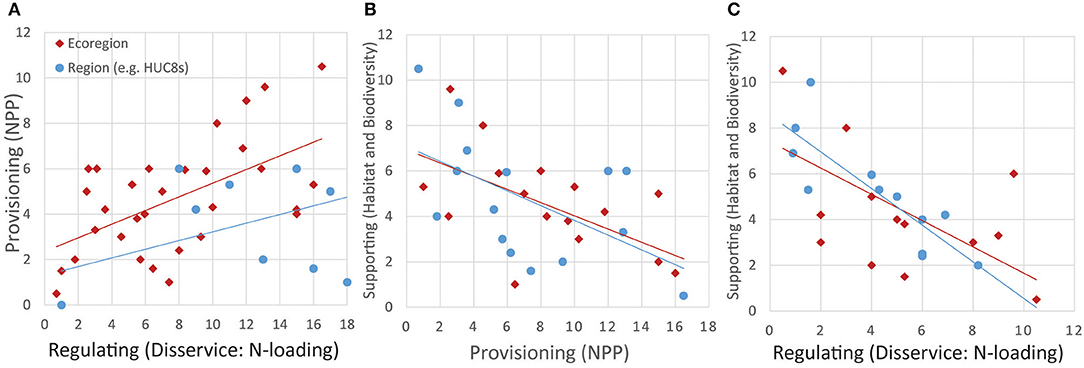
Figure 1. Hypothesized relationships, displayed as scatterplots and linear trendlines, among provisioning, regulating and supporting ecosystem services in the southeastern US, at ecoregion and regional (e.g., HUC-8) scales. Regulating services are represented as a disservice, e.g., nitrogen (N) loading of aquatic systems. Provisioning services are represented as net primary production (NPP). Supporting services are represented as measures of habitat and biodiversity. Ecoregional values (in red) were simulated as a bivariate distribution, and regional values were a random selection of the ecoregion. (A) Hypothesized positive relationship between regulating (disservices) and provisioning services at ecoregional (red) and regional (blue) scales. (B) Hypothesized negative relationship between provisioning and supporting services at ecoregional (red) and regional (blue) scales. (C) Hypothesized negative relationship between regulating and supporting services at ecoregional (red) and regional (blue) scales.

Materials and Methods

Study Area

This study compares ecosystem services documented at multiple scales in the southeastern US, from local to regional scales (Figure 2). At its broadest extent, the study area includes coastal plain regions extending from southern Virginia to southern Florida and west from coastal Georgia to the eastern bank of the Mississippi River, and into the alluvial plains in western Tennessee. The study areas associated with this research pertained to hierarchical spatial frameworks which allowed us to scale up measurements. Scaling-up started with the local scale and then moved up in area to regional frameworks in four steps. This scaling process resulted in a set of seven areas of interest, corresponding to regional spatial frameworks described below, whose locations were driven by two of the 18 USDA LTAR Network sites where we have field measurements.

FIGURE 2

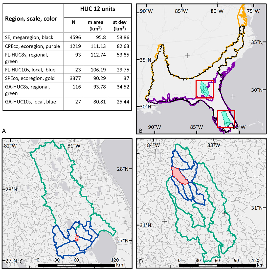
Figure 2. The southeastern US showing ecoregion and study area boundaries with HUC-12 unit summary. (A) Table describing study area names, scale, and map color, and showing count, mean and standard deviation of HUC-12 areas within the study area boundaries. (B) Southeast mega-region (SE, black outline), with Southeastern Plains Ecoregion (SPEco, gold outline), and Southern Coastal Plain ecoregion (CPEco, purple outline). (C) Florida study areas—FL-HUC8s (green outline), and FL-HUC10s (blue outline). (D) Georgia study areas—GA-HUC8s (green outline), and GA-HUC10s (blue outline).

Long-Term Agroecosystem Research (LTAR) Network Sites

For detailed local scale comparisons, we used two focal areas with comprehensive long-term measurements of production and other ecosystems services. First, the 4,200-ha Buck Island Ranch, managed by Archbold Biological Station, is one part of the ~12,000 ha Archbold-University of Florida LTAR site, referred to here as the ABS-UF. Buck Island Ranch lies within the beef cattle grazing lands of south-central Florida. Second, the 334 km² USDA-ARS Little River Experimental Watershed (LREW) instrumented by USDA for agricultural watershed experimentation and monitoring since 1968 (Bosch et al., 2007), lies at the heart of the Gulf Atlantic Coast Coastal Plain LTAR site south central Georgia. This site, comprised primarily of croplands, rivers and streams, and pine forests, is referred to here as the GACP.

Regional Frameworks

This analysis required us to summarize and compare data across the entire region and among subregions. To accomplish this, we used boundaries that describe hydrological characteristics and, at broader scales, ecological characteristics. We used the hierarchical Hydrologic Unit Code (HUC) system to establish the grain of our analysis (USGS, 2015) summarizing data from small area HUC-12 units (referred to here as HUC-12s), our most basic unit of analysis, within a grouping of HUC-10 units, and again within a larger area of several HUC-8 units. The number and area of HUC-12s incorporated into each scale step is given in Figure 2A. The HUC system is well-established and, for the scale of our analysis the HUC-12s provided a stable, consistent spatial framework allowing us to compare areas of increasing sizes, while maintaining consistency as we moved up and down the spatial hierarchy. At each scale increment, measurements from incorporated HUC-12s were summarized using simple descriptive statistics of central tendency and variability.

The first scale was conceptualized as an “LTAR Core” area, an area of local watersheds defined as the area of intersecting HUC-10 basins that include the GACP or ABS-UF sites, and we referred to as GA-HUC10s and FL-HUC10s, respectively. While we did not attempt to scale point measurements from either ABS-UF or GACP to these core areas, which would have involved an extensive amount of field verification, we used some local measures at these LTAR sites to verify the range of values observed in the HUC-level data.

For the second, regional scale, we selected a series of related HUC-8 regional basins that included our LTAR Core areas, but also related to a single larger HUC-6 level basin, and we referred to as GA-HUC8s and FL-HUC8s. In Georgia, the selected regional basins were all within the Suwannee Basin (HUC-6: 031102), and in Florida, the HUC-8s all pertain to the Kisimmee Basin (HUC-6: 030901). The rationale for study areas bounded by larger hierarchical units at this step, was to maintain a level of consistency in the assumptions underlying our analysis of ecosystem services and disservices. Because these measurement units relate to hydrology, the factor driving our decision to nest the smaller HUC-10 and HUC-8 study areas within a single larger HUC-6 region related to limiting the introduction of confounding issues of broader-scale cross-basin watershed dynamics.

The third scale involved a jump to the ecoregion level including most of the Southeastern Plains (SPEco), and the Southern Coastal Plain (CPEco) Level III ecoregions (Omernik and Griffith, 2014). A final, and fourth scale was the amalgamation of both ecoregions into a unifying southeastern US (SE) mega-region. At these larger regions, we initially defined the study area boundaries as the collection of HUC-12s which intersected the ecoregions. Further refinement led to a final subset of HUC-12s across the entire southeast, comprising 4,596 units. The entire list of HUC-12s used is provided in Supplementary Material 2—Data Table, and their area is identified by the black outline in Figure 2B. In some cases, such as the coastal plain of South Carolina and the rolling coastal plain of Virginia (north of the James River), HUC-12s were excluded from the SE, SPEco, and CPEco study areas because we judged them to be either highly uncharacteristic of our LTAR sites, or they were better represented by another LTAR site (e.g., Lower Chesapeake Bay LTAR). Units that intersected the boundary of the ecoregion were included if their centroids were within the ecoregion, but certain HUC-12s were excluded from the analysis if their land cover was mostly open water, such as large lakes or barrier islands.

Data

To accomplish this work, we identified several indicators of provisioning, regulating and supporting ecosystem services (or disservices), for which existing data were available at both the scale and grain required (Table 1, Supplementary Table 1.1). Source data for this analysis included published data available for download from public repositories (Supplementary Table 1.2), which we processed using geographic information systems (GIS; Esri, ArcGIS Pro 1.X - 2.X, and ArcGIS Desktop 10.6-7, Advanced licenses), and the Google Earth Engine (GEE) data and analysis platform. Boundary maps for contrasting regional analyses were created from the intersection of the hydrologic basin framework with the ecoregional framework as noted. Data describing land cover and ecosystem services consisted of gridded datasets produced and published in previous research or as operational land cover products. Basic criteria for these data included: scope—datasets had to be available for the CONUS, or for the entire SE mega-region; grain—datasets resolution had to be fine enough to provide estimations of land cover for areas >15 km², the size of the smallest HUC-12 basin included in the SE; and time period—data were fairly recent (within a decade).

TABLE 1

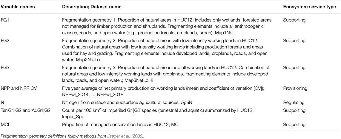
Table 1. Derived datasets used for analysis (see Supplementary Material 1 for sources and land cover reclassification; Supplementary Material 2—Data Table).

Land Cover

We used land cover information to compare the overall composition of land cover types for each region, and to estimate the fragmentation in landscapes within each study area, under three different characterizations of land use. For these analyses, we used both the USGS National Land Cover Dataset (NLCD) and the USDA Cropland Data Layer (CDL) datasets to derive information about land cover and land use in the region (Boryan et al., 2011; Yang et al., 2018; Jin et al., 2019). For our initial land cover characterization, we summarized land cover values for each study area using the NLCD, which does not include detailed categories of crop type. For this classification, we reduced the number of classes from 15 to 12 by combining “Barren” with open and low intensity “Developed” classes and combining medium with high intensity “Developed” classes. For subsequent, more detailed analysis inferring land use, we used the CDL data to differentiate finer categories of agricultural land cover type, as described below.

Ecosystem Service Indicators

Provisioning: Net Primary Production (NPP)

Provisioning ecosystem services were evaluated using net primary production (NPP) as an indicator of provisioning services from working lands. Although provisioning services can imply much more than simply NPP (or gross primary production, GPP)—for example, some consider yield to be a provisioning service—NPP is useful to describe a measure of biological productivity across widely divergent ecosystems (Running et al., 2000). In terms of ecosystem services, terrestrial primary production is considered the foundation of provisioning services directly related to agriculture, including production of food, fuel, and fiber (Smith et al., 2012), and the main reason for selecting NPP as one of the primary datasets to support the spatial scale of this analysis. There is a constant need to estimate values of terrestrial primary production at regional to global scales, and currently this is only possible by using remote sensing-based models. The traditional components for these estimates are GPP and NPP, where GPP is considered the total amount of carbon captured by plants while NPP defined as the amount of carbon allocated in plants after accounting for autotrophic respiration (Ruimy et al., 1994; Running et al., 2000).

Robinson et al. (2018) developed the Landsat-NPP model based on the MOD17 (MODIS-MODerate-resolution Imaging Spectroradiometer) algorithm (Haberl et al., 2007) producing a high-resolution (30 m pixel size) gridded dataset of annual NPP for the CONUS. This model relies mainly on the work developed by linking GPP and NPP to the amount of solar energy absorbed by plants along with atmospheric factors. Unlike the GPP product, which is produced at 16-days temporal resolution, NPP provides annual estimates that can be incorporated seamlessly into analyses requiring annual aggregation. The annual availability of NPP estimates along with the spatial resolution (30 m) and coverage (CONUS) made this satellite-based product the main candidate as a proxy of a provisioning ecosystem service indicator. We used mean annual NPP for 2014–2018 for this analysis. Data for NPP were tabulated for each HUC-12 area in units of kg carbon (C) per square meter. A mask of working lands was used to limit extract NPP data to areas associated with agricultural production. A more detailed description of the workflow and analytical methods used to calculate values for NPP is provided in Supplementary Material 1, 2.1.

Regulating: Nitrogen (N) Loading

To characterize regulating services, we considered the role of pollutant load, specifically agricultural nitrogen (N), as an indicator of the disservice provided by working lands. Landscape buffers adjacent to stream corridors provide important regulating services by purifying water running off intensively used lands. Where N is an essential macronutrient for primary production, and the most common ingredient in agricultural fertilizers, it is an environmental contaminant, so its measurement in aquatic systems indicates the extent to which the adjacent lands and soils are able (or unable) to purify water. Agricultural N concentrations in a watershed can serve, therefore, as an indicator of the effectiveness of regulating services within that area, where high N concentrations indicate a level of disservice.

The Environmental Protection Agency's (EPA) EnviroAtlas provides a nationwide data source for N concentrations to be used as a regulating service indicator. EnviroAtlas mapped modeled agricultural N (2002 values) removed by surface and subsurface flow (metric ton per HUC-12). These data were related to on-the-ground measurements from the LTAR sites after converting units to kg/ha. Data from ABS-UF were acquired from 4 years of collection in a field experiment between 1998 and 2003 (excluding 2000, a drought year) (Bohlen and Villapando, 2011). Data from GACP include N loading from stream collection data published for the LREW for 1978–2014 (Bosch and Sheridan, 2007; Bosch et al., 2020).

Supporting: Landscape Structure, Biodiversity, and Habitat

Supporting ecosystem services include habitat for species and the maintenance of genetic diversity. Numerous measures of biodiversity and habitat conditions exist, which can provide some indicator for the level of supporting services in a region. For this study, we used well-known indicators of both to describe supporting services. Habitat was characterized as the amount of land protected for conservation and by using landscape ecological indices to describe the fragmentation of natural and working lands. Landscape fragmentation is caused by landscape elements that bisect patches of otherwise habitable areas (usually single land cover or habitat types), or form barriers or impediments to landscape flows (Forman, 1995), including the movement of animals. Conversely, landscape connectivity is the result of landscape elements that facilitate connections, such as the ability of animals to disperse, mate and survive. While fragmentation per se is often associated with higher levels of biodiversity overall (Fahrig, 2017), landscape barrier characteristics strongly influence the nature and magnitude of fragmentation effects on animal species and populations. Roads are fragmenting elements (Rytwinski and Fahrig, 2013) with particularly negative effects on large carnivores such as Florida panther (Puma concolor coryi) and Florida black bear (Ursus americanus floridanus) (Ceia-Hasse et al., 2017; Murphy et al., 2017), both of which are endemic to the Southeast. For this study, biodiversity was characterized using outputs from habitat models for large regions, supported with counts of imperiled species in smaller areas. Together, these indicators provided different facets of supporting services and allowed for a more nuanced understanding of the comparative balance of ecosystem services associated with working lands in the Southeast.

Supporting: fragmentation, and landscape structure To understand the role of working lands in providing supporting ecosystem services related to wildlife especially terrestrial vertebrates, we characterized habitat using landscape ecological metrics and the area of “connecting elements” in each HUC-12. The landscape metrics used included patch number, area weighted mean patch area, and effective mesh size (McGarigal and Marks, 1995; Jaeger, 2000). Patch number is a well-known index of landscape structure that exhibits predictable patterns over a range of scales (Wu et al., 2000), and for which, increasing patch numbers are usually associated with increasing fragmentation over time, with implications for habitat connectivity and species diversity (Forman, 1995; Fahrig, 2003). Area weighted mean patch area (AWMPA), quantifies proportional amounts of patch area, and can be used to compare the proportion of habitat types in a management unit (McGarigal and Marks, 1995). In this case, however, we used it to compare the amount of patch (or habitat) area among analysis units. Effective mesh size (m_eff) characterizes fragmentation in a given unit of analysis, independent of its size (Jaeger, 2000), thus allowing for cross-scale comparisons. It incorporates scenarios based on land cover types permitting comparisons of alternative scenarios and assumptions, where negative correlations have been found between the degree of fragmentation and levels of species richness (Schmiedel and Culmsee, 2016).

We used land cover (CDL) and forest management data (Marsik et al., 2017, 2018) to derive datasets that characterized three levels of landscape fragmentation (Jaeger et al., 2008), described by increasing intensities of land use. To measure fragmentation, the geometry of fragmenting elements needs to be explicitly provided by stipulating the landscape elements that form the fragmentation geometry, or FG (Jaeger et al., 2008). “Fragmenting elements” comprise classes of land cover types that cause fragmentation in a landscape by breaking apart habitable environments. Conversely, the land cover classes that are not inhospitable are “connecting elements.” For example, urban areas, frequently used roads, and intensively farmed cropland are inhospitable for some species. However, the movements of other species may not be hindered by cropland, although their habitat may be fragmented by highways. Together, the spatial arrangement of fragmenting and connecting elements form the FG and are designated with a number differentiating the groupings of connecting and fragmenting elements, as in FG1, FG2, and so on. Final units of analysis included proportion of connecting elements in each HUC-12, and landscape metrics were described only for aggregated levels of analysis (i.e., -HUC10s, -HUC8s, ecoregion). A more detailed description of the workflow and analytical methods used to calculate values for landscape metrics, including the production of the FG layers is provided in Supplementary Material 1, 2.2.

Supporting: imperiled species Biodiversity is a key indicator of supporting services, describing, in general terms, the diversity of life that exists to support the long-term viability of populations and ecosystems, including the genetic building blocks that support livestock and cropping systems. While numerous measures of biodiversity exist, imperiled species data provide information to help gauge levels of biodiversity. EPA's EnviroAtlas provides a national map of the number of “At-Risk” species with potential habitat within each HUC-12 in the CONUS, which was used as one biodiversity indicator related to supporting services (US EPA, 2011). These data include species that are Imperiled, as defined by NatureServe (https://explorer.natureserve.org/AboutTheData/Statuses), or Listed under the US Endangered Species Act (ESA), and are indicated by the designation G1|G2. The values are based on habitat models, not wildlife counts, but could be compared with lists of known species for the ABS-UF area, and the list of G1|G2 species from the Georgia Biodiversity Portal, for the GA-HUC8s area (Georgia Department of Natural Resources, 2020). Both G1|G2 terrestrial species (EnviroAtlas: TR_TOT) and aquatic species (EnviroAtlas: AQ_TOT) were used for this analysis. The final datasets were counts weighted by the area of the HUC-12 unit providing a number per 100 square kilometers.

Supporting: habitat and lands protected for conservation Lands protected for conservation were also used as another indicator of biodiversity/habitat as a supporting service. To quantify this, we created a managed conservation lands (MCL) layer consisting of public lands as defined by the USGS Protected Areas Database of the US (PAD-US 2.0), and conservation easements documented in the National Conservation Easement Database (NCED) (https://www.conservationeasement.us). Conservation easements are important to include in this dataset because such lands support biodiversity and can cover large swaths of land, especially in Florida. We recognize that not all land trusts choose to share their conservation easements with the NCED due to lack of funding and technical capacity, or privacy concerns, and that it may vary from state to state (Rissman et al., 2019). This may present an unknown bias in Georgia, Alabama, and other states, however in Florida the area of easements acquired by land trusts are very minor in comparison to those held by state and federal agencies. The NCED draws from exhaustive mapping of all conservation “managed lands” by the Florida Natural Areas Inventory for the state. Based on reviewing known conservation easements in our areas we determined that the NCED was the best available region-wide dataset for our needs. Before combining these two datasets into one, we refined the PAD-US dataset to exclude US Department of Defense sites that were <10,000 acres and Recreation Management Areas from all public agencies, including water features such as lakes, rivers, and reservoirs, as these areas are not necessarily managed with a goal of supporting conservation. This combined dataset does not include other management practice incentive programs, such as the Conservation Reserve Program (CRP) and the Environmental Quality Incentives Program (EQIP) because the areas in those programs are afforded only a temporary conservation status. The final datasets consisted of the proportion of HUC-12s protected for conservation.

Analysis

It was not our intention to produce a multivariate statistical analysis of the cross-scale relationships among indicators, which would have introduced additional statistical challenges associated with the modifiable aerial unit problem (Fotheringham and Wong, 1991; Gotway and Young, 2002). However, we examined bivariate relationships between variables (Table 1), and compared the distributions of variables, plotting their kernel density functions to discover the likelihood of similarity between subregions and the larger regions within which they were nested (Scholz and Stephens, 1987).

Data preparation involved standardizing all datasets in the common HUC-12 spatial framework. Since national EnviroAtlas datasets (Agricultural N and Imperiled Species) are provided in this format, data preparation involved collating values from multiple attributes to calculate area-weighted summary measures of total N and G1|G2 species counts. Analyses of datasets included summary statistics over space and, for the NPP datasets, over a period of 5 years, including mean, median, standard deviation and CV. We then mapped and charted the spatial variability of summary measures to visually compare the study areas. We also conducted 216 pairwise bivariate regressions of the nine variables reviewed in this analysis to observe trends between variables at all scales (Supplementary Material 3).

Kernel density estimation was used as a non-parametric way to evaluate and compare the distributions of the datasets from the seven study areas for the nine indicators. The kernel density estimator (Silverman, 1986) of an unknown density f is given by:

$\begin{array}{l}{\widehat{f}}_h(x)=\frac{1}{n}{\displaystyle \sum _{i=1}^n}{K}_h(x-x_i)=\frac{1}{nh}{\displaystyle \sum _{i=1}^n}K\left(\frac{x-x_i}{h}\right)\end{array}$

where x_1,....,x_n is a sample drawn independently from the distribution with density f, h is the bandwidth, and K is the kernel. We used the function density() in the R base package (R Core Team, 2019) with its default settings, which include using a normal kernel.

Dataset density functions were statistically compared using the two-sample Anderson-Darling test (Scholz and Stephens, 1987), as implemented in the R (R Core Team, 2019) package kSamples (Scholz and Zhu, 2019). The null hypothesis for this test is that the samples come from the same (continuous) distribution. The test is based on the goodness of fit statistic of Anderson and Darling (1954) and is non-parametric—no underlying distribution needs to be specified. Such statistics often are used as a measure of distance between distributions or datasets. We used it in this sense to compare our datasets across scales (Supplementary Material 4).

To compare the indicator datasets for each LTAR study area, we constructed radar plots of the summary values of the HUC-12s. Values were normalized to a 0-1 scale within each category and plotted together in a radar plot configuration, providing a graphical comparison of the data space covered by ecosystem service indicators for each study area. This comparison included normalized values for: (1) mean annual NPP (primary production); (2) the inverted values of agricultural N loading (reduced N); (3) the ratio of FG1 to FG3 areas (proportion of natural lands within working lands); (4) the FG2 effective mesh size (a measure of connectivity); (5) the proportion of managed conservation lands (area conserved); and (6) terrestrial rare and imperiled species. Values for agricultural N were inverted prior to normalizing the scale so that values close to one indicated low levels of N runoff. This provided a consistent interpretive index where higher values could be associated with higher levels of ecosystem services to enable a visual comparison of tradeoffs and synergies.

Results

Land Cover and Working Lands Connectivity

Land Cover

Agricultural land covers in the study areas of the Southeast (Figure 3) are interspersed with extensive forests and wetlands. In the southernmost areas, agricultural land uses are associated with freshwater herbaceous wetlands, characteristic of humid, subtropical climates (Chen and Gerber, 1990; Beck et al., 2018) where water is a key driver. This association transitions to a coupling with riparian forested ecosystems as one moves northward. While the area of open water in the SE is only slightly greater than the US, 23% of the land area is covered with wetlands (herbaceous and woody) in the SE compared to about 6% for the US. These differences are even more marked for the CPEco, where 35% of the area is covered by these land cover categories. The other distinguishable feature of the SE is that the proportion of developed land classes is higher than the US, driven by high rates of urbanization in the CPEco where the amount of developed cover is 14.7%, more than double the US, and SPEco levels of 6.3% and 7.2%, respectively.

FIGURE 3

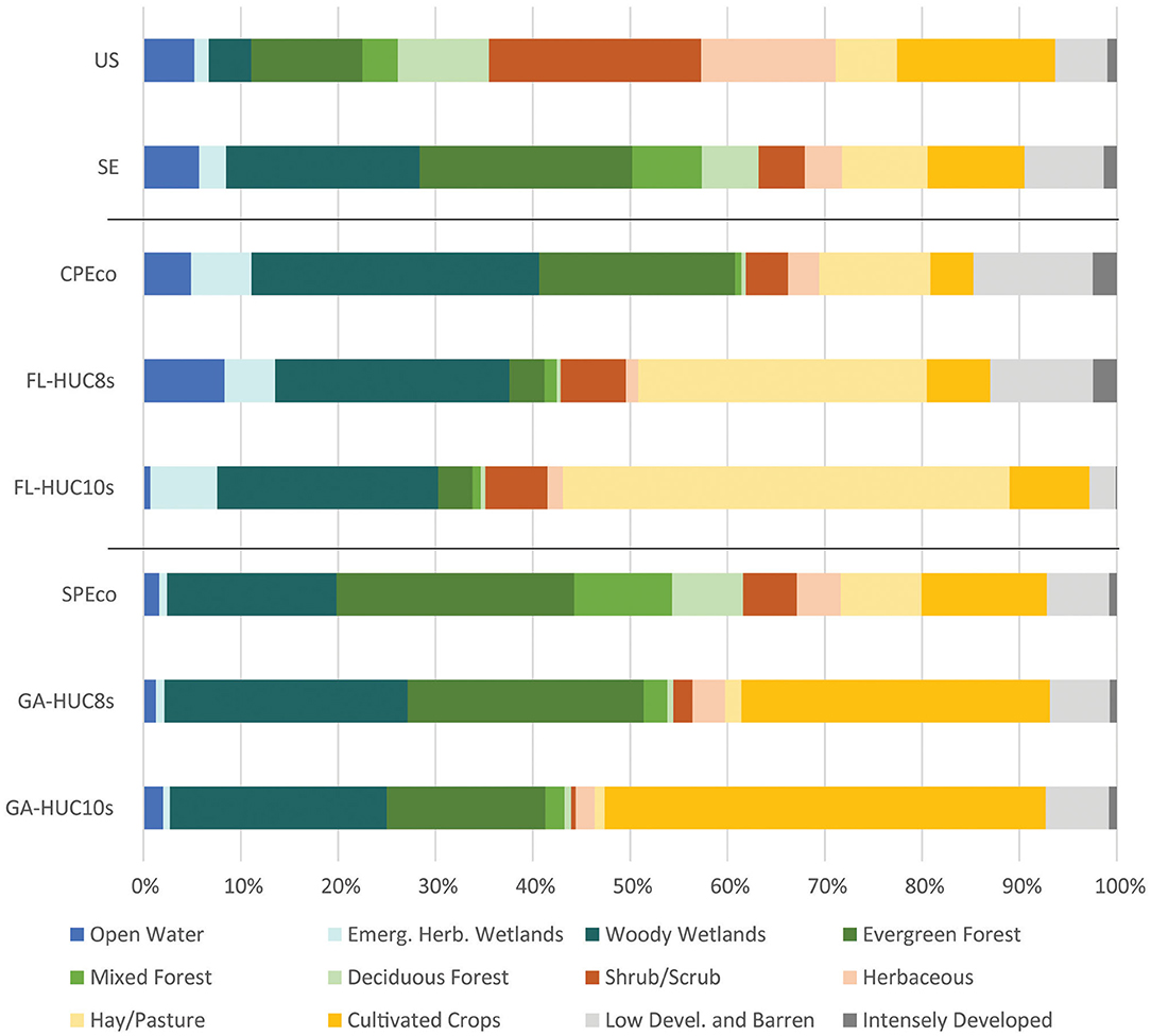
Figure 3. Proportion of land cover type by study region based on the 2016 USGS National Land Cover Database.

In the SE mega-region, cultivated crops and hay/pasture land covers ~19% of the area, slightly less than the US value of 23% (Figure 3). However, the proportion of these areas are lower in the southern ecoregion (CPEco = 16%), than the northern ecoregion (SPEco = 21%). At a smaller extent though, the regional basins (HUC8s) and local watersheds (HUC10s) are more dominated by crop and hay classes than the ecoregions they lie within. These lands occupy 36% of the FL-HUC8s study area and 33% of the GA-HUC8s area, increasing to 54% and 46%, respectively at the HUC-10s level. Of note is the shifting composition of crop and hay classes in moving down the hierarchy of focal areas. At the CPEco and SPEco levels, the proportion of crop and hay is fairly evenly split between the classes. However, at finer scales, hay/pasture classes dominate in the Florida study areas (30% of FL-HUC8s and 46% of FL-HUC10s), and cultivated crops in the Georgia study areas (32% of FL-HUC8s and 45% of GA-HUC10s).

Fragmentation and Connectivity of Working Lands From Landscape Metrics

Across the SE and its subregions, remaining natural areas, characterized here as FG1 connecting elements (gray areas in Figure 4), occupy, on average, about a third or less of HUC-12 areas, except for HUC-12s in the CPEco study area, where the average area of connecting elements is over 40% (Supplementary Table 1.6). Despite having 30–40% of the landscape in natural areas, the southeastern US is highly fragmented, as demonstrated by high numbers of patches and low m_eff. This value changed markedly across all study areas upon the inclusion of low intensity working lands as connecting elements (i.e., FG2), when the proportion of connecting element area increased substantially to more than 50% (Figure 5). For all study areas, the number of patches declined substantially, while patch size and m_eff increased (Figure 5). Trends for AWMPA were nearly identical to those for m_eff. This was especially true in the SPEco, where production forestry is so common and those uses tend to be highly interspersed more “passively” managed areas. Generally, fragmentation is more pronounced in the Georgia study areas, however, the inclusion of low intensity working lands provided a critical “boost” to connectivity in local watersheds of both Georgia and Florida study areas (GA-HUC10s and FL-HUC10s). In Georgia, the increase in connectivity was clearly due to the inclusion of riparian forests in the analysis (Figure 4), while in Florida, the inclusion of grasslands used for pasture was the key factor increasing levels of landscape connectivity.

FIGURE 4

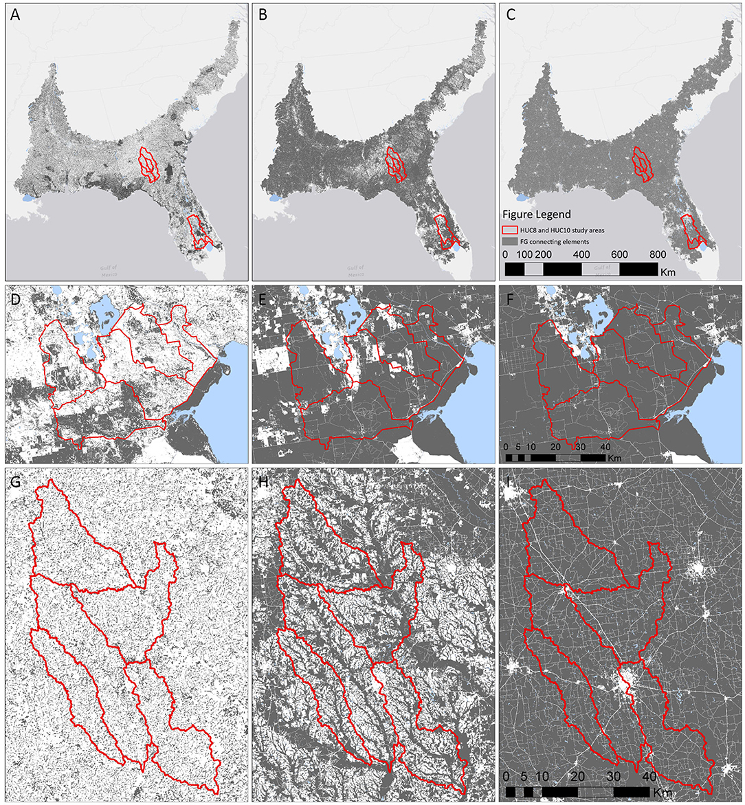
Figure 4. Land use fragmentation geometries (FGs) in the southeastern US (top row), Florida (center row), and Georgia (bottom row), with increasing intensity of use (columns). Left column shows FG1, consisting of wetlands, shrublands and unmanaged forests (gray) for the Southeast (A), Florida (D), and Georgia (G). Middle column shows FG2, consisting of areas in FG1 plus all forests, shrublands, grasslands, and hay production areas (gray) for the Southeast (B), Florida (E), and Georgia (H). Right column shows FG3, consisting of areas in FG2 plus croplands (gray), for the Southeast (C), Florida (F), and Georgia (I), so that areas excluded (white) are developed and open water land cover classes. See Supplementary Material 1 for land cover classification and GIS workflow.

FIGURE 5

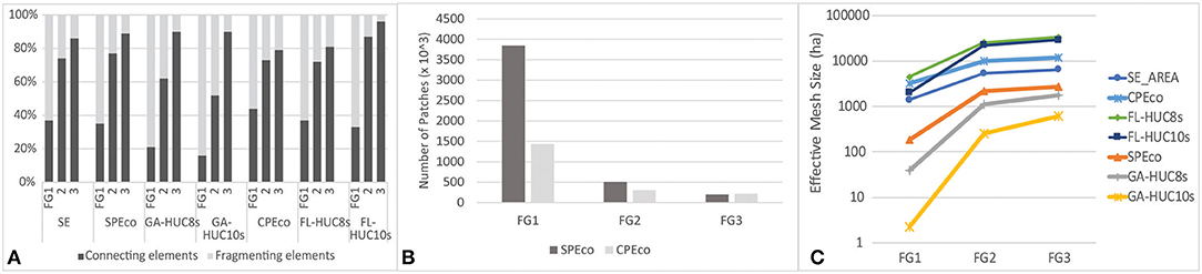
Figure 5. Landscape ecological indices of connectivity and fragmentation for three fragmentation geometry (FG) levels. (A) Proportion of total mean HUC-12 area of connecting vs. fragmenting elements for each study area and for each FG level. (B) Graph of number of patches by ecoregion. (C) Graph of effective mesh size (m_eff). Tabulated data provided in Supplementary Table 1.6.

Including all working lands (high intensity croplands as well as low intensity) in FG3 effectively reduced fragmenting elements to a very small proportion of the overall landscape with the exception of the Florida ecoregion (CPEco) and regional basins (FL-HUC8s). These are, however, areas where hard urban edges, including roads, form substantial fragmenting elements and represent a significant proportion of developed land cover classes, keeping connecting elements to about 80% of the landscape.

Spatial Variability of Ecosystem Service Indicators

Provisioning Services Characterized by NPP on Working Lands; Mean and CV Over Time

Net primary production (NPP) in the SE generally varied considerably over space and from 1 year to the next during 2014–2018. The data were normally distributed with mean and median values closely related. The five-year mean of annual NPP averaged across the SE study area was ~7,176 kg C/ha and the mean CV was 5.8%. The range of CV (1–13%) for working lands in the SE stands in contrast to the CV of 4–38% for the entire 1987–2018 dataset, which includes all years and all pixels. General comparisons (Figure 6) of the data show that NPP in the Florida HUC-12s was far more variable than in the Georgia HUC-12s, especially within the local study areas. In Georgia, NPP was consistently higher and far less variable. While ecoregional CV values in both ecoregions ranged widely, variability for the regional basin and local watershed areas in Georgia (i.e., GA-HUC8s and GA-HUC10s) were far lower than the ecoregional means, an unsurprising result related to the modifiable areal unit problem, previous mentioned. Within the LTAR sites, GPP was measured from eddy-covariance flux towers. At the ABS-UF site, annual GPP was measured in 2013–2015 at 24.589, 17.995, and 16.131 Mg C/ha in improved pastures, semi-native pastures and wetlands, respectively (Chamberlain et al., 2016; Gomez-Casanovas et al., 2018). Similar values were reported at the GACP site where in 2016, annual GPP for miscanthus and maize were 30.73 and 26.43 Mg C/ha, respectively (Maleski et al., 2019). While these data do not account for respiration C losses, they provide ground validation of production within the study areas, and indicate similar levels of production for the areas of working lands in Florida and Georgia.

FIGURE 6

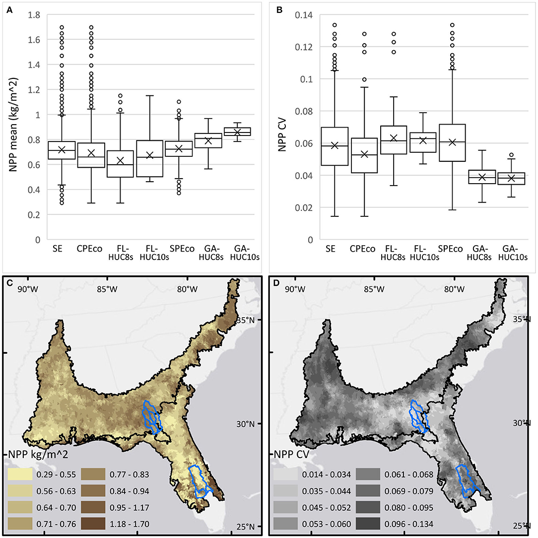
Figure 6. Boxplots and maps of net primary production (NPP, kg C/m²) and coefficient of variation (CV%) average annual mean values, 2014–2018, calculated for HUC-12 areas and summarized for each study area (clockwise from top left). (A) Boxplots of NPP for each study area. (B) Boxplots of NPP CV for each study area. (C) Map of NPP calculated for HUC-12s in the Southeast (SE). (D) Map of NPP CV calculated for HUC-12s in the Southeast (SE). Blue outlines show HUC-8 areas.

Regulating Services Characterized by Nitrogen Runoff

Modeled values of agricultural N runoff (Figure 7) in the SE mega-region were skewed right with a median of 3 kg/ha, and the top 1% with values of 70–260 kg/ha. In ecoregions the median values were lower in CPEco than SPEco (1.5 and 3.5 kg/ha, respectively) but overall values were more variable in the CPEco where the SE maximum value was found, well-exceeding that of SPEco maximum of 183 kg/ha. At the regional basins and local watershed extents (HUC8s and HUC10s), the extreme values were more constrained but, the study areas in Florida had higher median N runoff estimates and greater variability. At the ABS-UF study site, based on pretreatment data for eight pastures from a previous study. average annual values of total N were 9.155 kg/ha (see Bohlen and Villapando, 2011). In Georgia, riparian forests are well-established throughout the area, particularly in the local watersheds region (GA-HUC10s), serving as buffers for agricultural runoff, and resulting in lower N runoff in streams. This is consistent with the GACP measured N loading values published for the LREW of ~4.2 kg/ha for 1978–2014 (Bosch et al., 2020). For one HUC-12 located in Florida, N values were extremely high, which may have skewed trends slightly in the CPEco, and, based on personal knowledge of this area, we suspect this was an aberrant value in the dataset of 4,596 records.

FIGURE 7

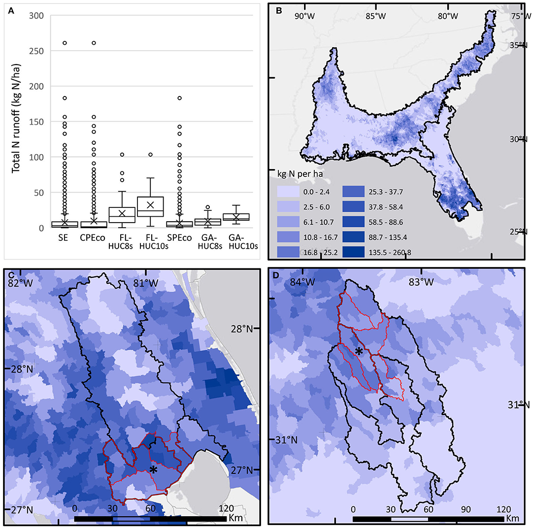
Figure 7. Boxplots and maps of modeled agricultural nitrogen runoff (N, kg/ha) calculated for HUC-12 areas and summarized for each study area. (A) Boxplots of N for each study area. Asterisk (*) shows location of LTAR sites. (B) Map of N calculated for HUC-12s in the Southeast (SE). (C) Map of N calculated for HUC-12s in the Florida study areas. (D) Map of N calculated for HUC-12s in the Georgia study areas.

Supporting Services Characterized by

Imperiled Species

The distributions of G1|G2 imperiled aquatic and terrestrial species varied markedly across the SE mega-region. The EnviroAtlas data show the CPEco ecoregion supports higher values for both terrestrial and aquatic imperiled species, with terrestrial species strongly associated with scrub and sandhill habitats of the peninsula's ancient sand ridges, as well as the Apalachicola and Ocala National Forests, and aquatic species closely associated with springs habitat in the northern peninsula (Figure 8, Supplementary Figure 1.2). Buck Island Ranch, at the ABS-UF site, supports four G3 species but no G1|G2 species, although it has five federally threatened and endangered species on site. It also lies within a region of the CPEco, where many HUC-12 watersheds within the regional basins (FL-HUC8s) are each associated with 5+ imperiled species (Figure 8C), a nationally high level of rarity. Working lands in Florida both directly support and are embedded within a region of high conservation value for rare species.

FIGURE 8

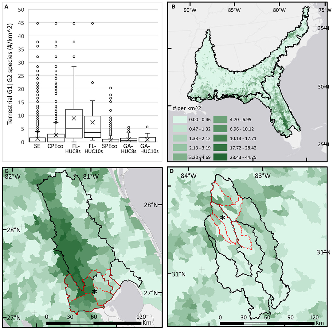
Figure 8. Boxplots and maps of numbers of rare and imperiled terrestrial species (G1|G2) calculated for each HUC-12 (n /100 km²) and summarized for each study area (clockwise from top left). Asterisk (*) shows location of LTAR sites. (A) Boxplots of terrestrial G1|G2 species for each study area. (B) Map of terrestrial G1|G2 species calculated for HUC-12s in the Southeast (SE). (C) Map of terrestrial G1|G2 species calculated for HUC-12s in the Florida study areas. (D) Map of terrestrial G1|G2 species calculated for HUC-12s in the Georgia study areas.

Conversely, the EnviroAtlas data suggest that the SPEco ecoregion supports lower numbers of terrestrial imperiled species; the GACP site has no known G1|G2 terrestrial species listed. Although the data show that areas in the local watersheds are estimated to have either one or no G1|G2 terrestrial species, Georgia Biodiversity Conservation Data (https://georgiabiodiversity.a2hosted.com) suggests that each of the HUC-8s within the GA-HUC8s regional basins host 2–3 terrestrial G1|G2 animal species, and 3–5 similar plants species, an apparent contradiction of the datasets. Even though our study area excluded the coastal HUCs from both ecoregions, the SPEco clearly supports many rare G1|G2 aquatic species in inland riverine and headwater basins (Supplementary Figure 1.2). These freshwater systems and stream corridors with rare aquatics raise important challenges for working lands that may affect downstream water quality.

Lands Protected for Conservation

In the SE mega-region, the average proportion of HUC-12s protected for conservation is <11% (Figure 9). However, this proportion protected is heavily right-skewed, with 50% of the HUC-12s having <1.5% of their areas protected for conservation.

FIGURE 9

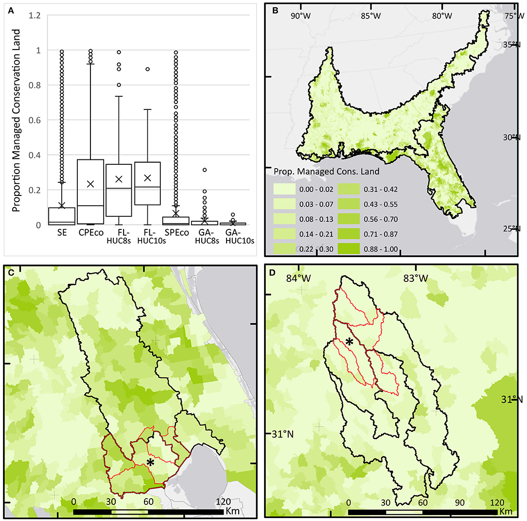
Figure 9. Boxplots and maps of percent area of lands protected for conservation calculated for HUC-12 areas and summarized for each study area (clockwise from top left). Asterisk (*) shows location of LTAR sites. (A) Boxplots of percent area of lands protected for conservation for each study area. (B) Map of percent area of lands protected for conservation calculated for HUC-12s in the Southeast (SE). (C) Map of percent area of lands protected for conservation calculated for HUC-12s in the Florida study areas. (D) Map of percent area of lands protected for conservation calculated for HUC-12s in the Georgia study areas.

There is an extreme disparity evident between HUC-12 areas primarily in Florida vs. those in Georgia. Both areas have many HUC-12 units with <2% of the area in conservation lands. However, in the CPEco, half of HUC-12 units in the region have 11% or more of their area protected for conservation, and at the scale of the FL-HUC8s and HUC10s, many HUC-12s include over 20% of their land protected for conservation. Working lands in the FL LTAR Core region lie within an extensive landscape of public and private conservation lands.

In contrast, although the SPEco includes a few HUC-12s with substantial areas protected, the majority of HUC-12s have <1.4% of their area in protected status, less than the SE generally. The low proportion of land protected for conservation in the ecoregion is especially evident in the regional basins (GA-HUC8s), where only a handful of HUC-12 units include any land protected for conservation, and the majority have none. Working lands in the GACP region and their embedded natural areas represent the most valuable areas remaining for conservation although they are unprotected.

Distributions of Ecosystem Services Across Scales

Bivariate Pairwise Comparisons of Selected Ecosystem Services

Of the 216 pairwise comparisons of ecosystem service indicators at different scales, a subset is included here (Figure 10) to illustrate results related to our hypothesized relationships (Figure 1). The full collection of pairwise comparisons is included in Supplementary Material 3.

FIGURE 10

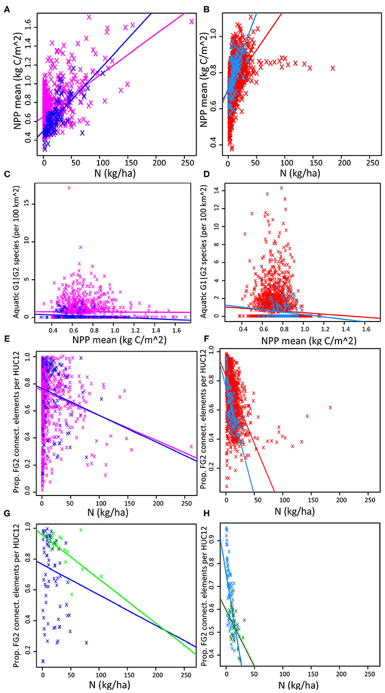
Figure 10. Pairwise comparisons of selected ecosystem service indicators (Supplementary Material 3). (A) Provisioning vs. Regulating: Mean NPP, 2014–2018 (kgC/m²) vs. Agricultural N runoff (kg/ha¹), in CPEco (magenta, n = 1,219), and FL-HUC8s (blue, n = 94) study areas. (B) Provisioning vs. Regulating: Mean NPP, 2014–2018 (kgC/m²) vs. Agricultural N runoff (kg/ha), in SPEco (red, n = 3,377) and GA-HUC8s (dodger blue, n = 116) study areas. (C) Supporting vs. Provisioning: Aquatic G1|G2 species (n/100 km²) vs. Mean NPP, 2014–2018 (kgC/m²), in CPEco (magenta, n = 1,219), and FL-HUC8s (blue, n = 93) study areas. (D) Supporting vs. Provisioning: Aquatic G1|G2 species (n/100 km²) vs. Mean NPP, 2014–2018 (kgC/m²), in SPEco (red, n = 3,377) and GA-HUC8s (dodger blue, n = 116) study areas. (E) Supporting vs. Regulating: Proportion of FG2 connecting elements vs. Agricultural N runoff (kg/ha), in CPEco (magenta, n = 1,219), and FL-HUC8s (blue, n = 94) study areas. (F) Supporting vs. Regulating: Proportion of FG2 connecting elements vs. Agricultural N runoff (kg/ha), in SPEco (red, n = 3,377) and GA-HUC8s (dodger blue, n = 116) study areas. (G) Supporting vs. Regulating: Proportion of FG2 connecting elements vs. Agricultural N runoff (kg/ha), in FL-HUC8s (blue, n = 94), and FL-HUC10s (green, n = 23) study areas. (H) Supporting vs. Regulating: Proportion of FG2 connecting elements vs. Agricultural N runoff (kg/ha), in GA-HUC8s (dodger blue, n = 116), and GA-HUC10s (forest green, n = 27) study areas.

Regulating vs. provisioning services: N loading vs. NPP As hypothesized, downstream N loading increased with increasing NPP productivity at the ecoregion, regional basin, and local watershed scales. NPP was higher in general in the SPEco than in CPEco, and more HUC-12s had both high productivity and low downstream N loading in SPEco (Figures 10A,B). Drilling down, the GA-HUC8s (regional) and -HUC10s (local) had lower modeled N loadings than the Florida areas, and the relationship with NPP was clearer, appearing asymptotic at lower N levels in Georgia versus Florida. The variance in NPP (NPP_CV) showed an apparent negative relationship with NPP in Florida, potentially driven by the variability in grassland productivity, vs. no obvious relationship in Georgia.

Supporting vs. provisioning services: aquatic biodiversity vs. NPP A high proportion of Florida and Georgia HUC-12 units had zero aquatic imperiled species (AqG1|G2) present, but in contrast to predictions for both ecoregions, there were more AqG1|G2 species at intermediate NPP levels (Figures 10C,D) although there was a longer right tail with low AqG1|G2 numbers at high N for Florida HUC units. The same broad pattern of more rare aquatic species at intermediate NPP values could be seen at all landscape scales from local watersheds (HUC10s) to the SE mega-region.

Supporting vs. regulating: FG2 vs. N loading The combination of natural areas with low intensity working lands (described by FG2) means there is a higher proportion of contiguous land covers available for regulatory ecosystem services. As expected, there was a negative relationship between the proportion of these areas and N loading (Figures 10E,F). This effect was observable at all scales from local watersheds to the entire SE but was most marked in Georgia regional basins and local watersheds (GA-HUC8s and -HUC10s, respectively; Figures 10F,H) These areas help buffer streams and offset the N loading effects, as found in other published studies from this region (Lowrance et al., 1984; Bosch et al., 2020; Pisani et al., 2020).

Kernel Density Functions of Ecosystem Services Across Scales

While box plots (Figures 6–9) allow for visual comparisons of the mean and variance for selected ecosystem service indicators, the Anderson-Darling test was used to test the goodness of fit or distance between pairs of kernel density functions in the datasets (Scholz and Stephens, 1987). We produced 81 pairwise comparisons (nine variables × nine scale pairs), of which, only 17% had similar density distributions (i.e., larger P-values; Supplementary Material 4) suggesting that most ecosystem services do not scale concordantly. In cases where concordant distributions were found, this was most often among the smaller local, HUC-10, and regional, HUC-8, areas (Figure 11). The distribution of mean NPP values in the local watersheds and regional basins of Florida were similar, which was, in turn, similar to the CPEco ecoregion (Figure 11A), unlike the Georgia extents which were all dissimilar (Figure 11B). The distribution of CV values, describing the variability in mean NPP, was also similar among the smaller extents both in Florida and Georgia (Supplementary Table 4.2). Although the records of G1|G2 species include many 0 values, the distribution in the Florida local and regional basins (FL-HUC10s and -HUC8s; Figure 11C) were smooth with low numbers of species. In contrast, the GA-HUC10s and -HUC8s (Figure 11D) were similar, but distributions were spiky because of large numbers of zeroes. The distributions of the proportion of FG2 connecting elements were similar in the CPEco and FL-HUC8s but were dissimilar at other scales in Florida and Georgia (Figures 11E,F). However, the proportion FG3 connecting elements were similar for the smaller extents in Georgia (Supplementary Table 4.9).

FIGURE 11

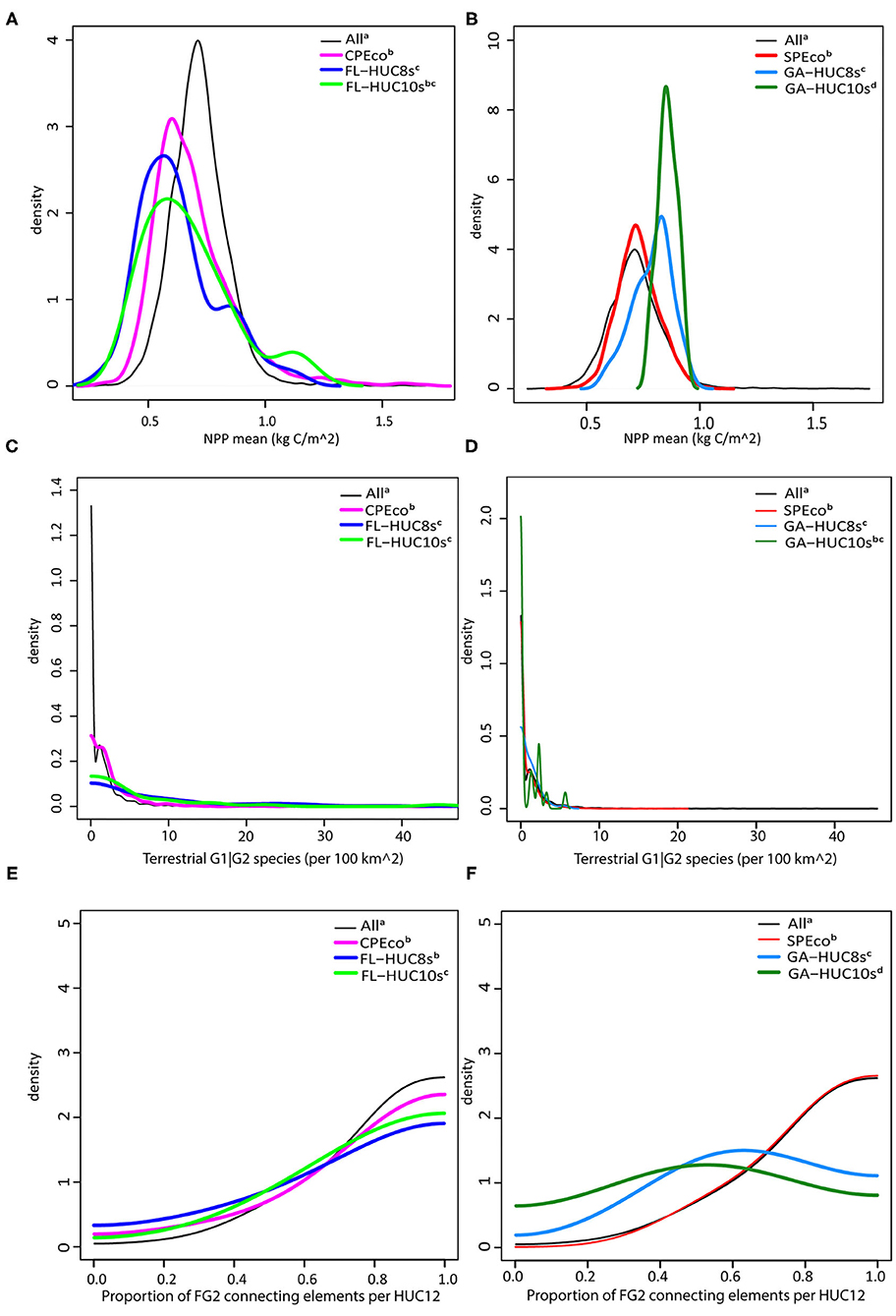
Figure 11. Kernel density function comparisons where superscripts indicate similar distributions (Anderson-Darling statistic P > 0.05; Supplementary Material 4). (A) Mean NPP (kg C/m²)—all data with Florida sub-regions. (B) Mean NPP (kg C/m²)—all data with Georgia sub-regions. (C) Terrestrial Imperiled Species (n/100 km²)—all data with Florida sub-regions. (D) Terrestrial Imperiled Species (n/100 km²)—all data with Georgia sub-regions. (E) Proportion of FG2 connecting elements—all data with Florida sub-regions. (F) Proportion of FG2 connecting elements—all data with Georgia sub-regions.

Multivariate Comparison of Ecosystem Services in Radar Plots

Radar plots showing a graphical representation of six values of ecosystem service indicators illustrated the tradeoffs and synergies among these services (Figure 12; Supplementary Table 1.3). Not surprising, ecosystem services derived from the SPEco, totaling 70% of the SE, were more similar to those from the entire SE mega-region than services from the Florida ecoregion (CPEco), which represents the remaining 30%. The balance of ecosystem services is not evenly distributed across the SE.

FIGURE 12

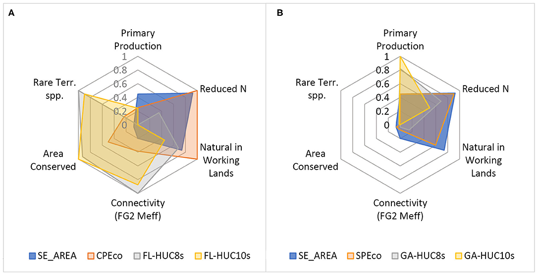
Figure 12. Radar plots of six ecosystem service indicators for each of seven ecosystem service indicators: (clockwise from top) Primary production (mean NPP); Reduced N, the inverse of agricultural nitrogen runoff; Natural in Working Lands (ratio FG1:FG3); Connectivity (FG2 m_eff, effective mesh size of the FG2 connecting elements, i.e. natural areas and low intensity working lands); Area Conserved (prop. MCL, proportion of lands protected for conservation); and Rare Terrestrial Species (TerrG1|G2, terrestrial G1|G2 imperiled species). (A) Florida study areas: SE megaregion, CPEco ecoregion, FL-HUC8s regional basins, and FL-HUC10s local watersheds. (B) Georgia study areas: SE megaregion, SPEco ecoregion, GA-HUC8s regional basins, and GA-HUC10s local watersheds.

Compared with the Georgia ecoregion (SPEco) and the SE, the local watersheds and regional basins (GA-HUC10s and -HUC8s) appeared quite different, showing higher productivity and higher agricultural N runoff (lower values on the radar plot) than mega-regional median values. In terms of habitat and biodiversity indicators, they were similar to the values for the SE or the SPEco. But they differed in that a greater proportion of working lands were high intensity croplands as opposed to the less intensive, but more extensive, production forests found in the rest of the SPEco.

In the local watersheds and regional basins of Florida (FL-HUC10s and -HUC8s), productivity was extremely low, and yet these areas still showed higher downstream N loading. However, the Florida regions showed high levels of supporting services, as measured by conservation indicators, with more rare species, a greater proportion of conservation lands, and large patch sizes within low intensity working lands. In one respect the local watersheds in Florida were more similar to the SE study area overall and differed from Georgia, retaining a higher proportion of natural areas within working lands. Comparing this value on the radar plots for both SPEco and CPEco regions, the CPEco had the effect of “pulling” the entire SE to a higher rank on the axis. Likewise, higher values for NPP in the SPEco, such as seen in the GA-HUC10s and -HUC-8s presumably had the effect of pulling the SPEco region to higher levels on the NPP axis.

Discussion

Globally the agricultural sector is challenged to no longer simply maximize productivity, but rather to optimize across multiple goals including environmental stewardship, and the prosperity and well-being of rural communities (Pretty et al., 2010). Optimization requires a better understanding of the contributions of working lands toward multifunctional ecosystem services at local, regional and national scales (Petersen and Snapp, 2015). We described the tension resulting from this optimization with the image of the fictional “pushmi-pullyu” character in the Introduction, in which some land management actions “pull” ecosystem services, while at the same time unintentionally “pushing” disservices. But, in terms of the overall balance of ecosystem services, the pushmi-pullyu character has only two heads and no scaling issues, whereas comparative analyses of synergies and trade-offs among production and other ecosystem services cannot ignore issues of scale and complexity. The challenge to analyze tradeoffs and synergies of ecosystem services in working lands is more complex, and requires a framework for scaling, analysis, and comparison. While the ecosystem services framework provides a unifying concept for comparing diverse outcomes from agroecosystems, the HUC spatial framework is useful for evaluating how well these ecosystem services do or do not scale. This research constitutes an attempt by two LTAR sites in a common geographic zone to compare outcomes of ecosystem services, probing the limits of how representative they are of the larger context, an understanding which is essential for accomplishing the Network's goals related to national scale agroecological research.

We selected the HUC-12 hydrologic unit (USGS, 2015), as the spatial grain for comparing multiple empirical and modeled datasets across scales, from site to regional areas of interest in the southeastern US. In this, we were strongly influenced by US EPA (2011) which also used the HUC-12 for its nationwide analysis. Our analysis used areal measurements of indicators to summarize and characterize regions, and so, an alternate selection of boundaries would have likely changed our characterizations of the regions, (Fotheringham and Wong, 1991). However, our selection of regions was not arbitrary, but was based on indicators for which we had relatable in situ measurements from the two LTAR sites in Georgia and Florida, and which related to the ecoregional and hydrologic frameworks of our analyses.

After considerable evaluation of available data, we chose five factors to derive nine indicators of provisioning, regulating and supporting ecosystem services, for which we could acquire empirical data throughout the southeastern US at the HUC-12 grain of analysis. Ultimately, we used: (1) net primary production (annual mean and CV), (2) agricultural Nitrogen runoff, (3) imperiled species (terrestrial and aquatic), (4) the proportion of areas managed for conservation, and (5) connecting landscape elements (three types). While we used land cover data extensively in this analysis, land cover characterization was one result used to compare study areas, and these data were combined with other datasets as described in our methods and in Supplementary Material 1.

Characterizing Ecosystem Services Associated With Working Lands

Our characterization of ecosystem services associated with working lands in the Southeast was constrained to those for which we were able to produce adequate datasets that followed across scales for all our study areas. Provisioning was characterized by mean annual NPP, and mean CV of NPP (over 5 years) since otherwise aligning crop yields and grassland productivity is challenging. Regulating services were indicated by agricultural N (modeled), an ecosystem disservice that we inverted for consistency in the radar plot comparison (less N = high service). Other ecosystem service indicators are of great interest, such as pollinator populations or species biodiversity but to date these lack complete spatial coverage and often do not incorporate data from working lands. Similarly, although we had some habitat specific data on greenhouse gas emissions from our LTAR research, it was not enough to characterize regulatory services over the heterogeneity of an entire HUC-12 around a LTAR site for comparative purposes. We fell back on the supporting services of species rarity (G1|G2 species), the proportion of conservation lands protected, and landscape factors, including the proportion and connectivity of natural lands vs. agricultural lands.

Indicators of provisioning services in the CPEco and SPEco demonstrated the variability of production in the region (Figures 6, 10A,B). The agricultural regions of Georgia, described by the GA-HUC10s and -HUC8s, generally occupy the higher ranges of mean NPP values in the region, while those of Florida, in the FL-HUC10s and -HUC8s, are in the lower ranges, and are much more variable. Together, production values from these two smaller areas in Georgia and Florida, coincident with the LTAR Network sites, cover the range of NPP values in all but the most extreme outliers of the SE. While the distribution of mean NPP values was similar only among the Florida study areas, the amounts of change within those annual mean values, as described by CV, was similar between local scales (-HUC10s and -HUC8s) in both Florida and Georgia.

Regulating services in working lands of the Southeast are provided largely in the natural areas buffering riparian and aquatic systems throughout the region. This effect is seen wherever “natural” lands and low intensity working lands follow adjacent to waterways. The distribution of N runoff values in our local and regional study areas were higher than the overall SE region. Keeping in mind that both the FL-HUC10s and GA-HUC10s study areas comprise mostly agricultural lands cover classes at more than twice the proportion than the SE (Figure 3), the difference in distributions of total N runoff values is not surprising.

The southeastern US is distinguished by highly heterogenous land covers with natural areas that are strongly associated with forested and wetland land covers. Together these natural lands total 37% of the southeastern US study area, well in excess of the 30% for the continental US. Services derived from less intensive agricultural land uses as well as from silviculture generally have fewer environmental costs than intensive agricultural operations (Power, 2010). In the southeastern US, when we combined these less intensive working lands with natural habitats (Figure 4) the extent of the landscape from which supporting ecosystem services could be expected essentially doubled from 37 to 74% (Figure 5, Supplementary Table 1.6). This percent was similar in the two ecoregion study areas: 77% of the SPEco, and 73% of the CPEco. Further considering this addition, the spatial configuration of the “ecosystem service landscape” was transformed, with patch areas providing services greatly increased, and fragmentation decreased.

Largely in response to the pressures of urbanization, another human dimension that will affect drivers of ecosystem services, more land is protected for conservation in the CPEco than SPEco (23 vs. <2%). This stems from decades of massive investment in public land acquisition and purchase of conservation easements in Florida by the federal government and the state (Farr and Brock, 2006). In comparison, with fewer conservation land purchases by the state of Georgia and elsewhere in the southeastern coastal plain, remaining natural habitats important for ecosystem services lie disproportionately within working lands and are typically unprotected.

Trade-Offs and Synergies of Landscape-Scale Ecosystem Services

Results from the pairwise comparisons of services (provided in Supplementary Material 3) were broadly in the directions predicted (Figure 1) and showed the same general patterns from the local (-HUC10s) to the ecoregion scale, although the trendlines for the relationships were often markedly different in the CPEco region in Florida other parts of the SE (Figure 10).

The impacts of the inclusion of working lands, and particularly the shift to combine connectivity of natural areas with low intensity and then high intensity working lands (from FGI to FG2 and FG3), highlights obscured environmental service levels at different landscape configurations. Pairwise comparisons of productivity against an increasing proportion of the connected landscape in an ecoregion, from FGI to FG2, then to FG3, showed: first, a strong negative relationship, i.e., lower productivity with a high proportion of natural areas (FG1); then, a weaker but still negative relationship when low level intensity agricultural lands were added (FG2); and finally, the expected steep positive asymptote for high productivity with all agricultural lands (FG3) included. The relationships are more extreme in the SPEco region with more croplands than the CPEco in Florida. Similarly for N runoff comparisons, going from the FG1 to FG2-configured landscape, shows the respective transition from a negative relationship with a high amount of natural areas (more natural areas, less N) to a mixed relationship depending on the ecoregion (slightly positive in CPEco, slightly negative in SPEco). Subsequently the FG-N relationship becomes obviously positive with the inclusion of high intensity agricultural lands.

Other data also indicate differences in ecosystem service trade-offs, for example the extensive semi-native grazing lands and scattered seasonal wetlands in Florida support high biodiversity including rare species, but yet these regions still produce high downstream N loadings. While croplands in Georgia have high productivity, streams and forested wetland habitats dissect the landscape, buffering and lowering N nutrient loading from adjacent crop fields, revealing a synergistic relationship among regulating and supporting services in these regions.

Representativeness of USDA LTAR Network Sites

To accomplish the task of understanding the interactions among indicators in broad domains of production, environment, and rural well-being in US agroecosystems (Kleinman et al., 2018), it is necessary to characterize the LTAR Network locations. For the two LTAR sites included in this study, ABS-UF (Florida) and GACP (Georgia), our data and analyses addressed two aspects of representativeness of the regions in which they lie. First, we quantified their landscape configurations and ecosystem services, including comparisons with site-specific data collection at the LTAR locations. Second, we characterized the tradeoffs and synergies among ecosystem services at the LTAR sites versus the increasing spatial extents across the region.

For the ecosystem service indicators we analyzed, observations measured within the LTAR sites fell within the ranges of observed or modeled data values. For those indicators, we concluded that the LTAR sites were represented well by the data summarized in the HUC-12s immediately surrounding the LTAR, i.e., the LTAR Core areas, or local watersheds (Figures 2C,D), and to some extent the broader regional basins, or -HUC8s.

Our analyses showed how the two LTAR Core areas represent specific conditions of agriculture-dominated watersheds within the range of values encountered in the southeastern US. Given the huge variability evident in the data for the SE, it is not surprising to find that the ABS-UF and GACP LTAR sites are not representative of the whole. But we have found that, regionally, measurements at these sites offer a good representation of the surrounding watersheds. This conclusion was enabled by the hierarchical nature of the analysis and our ability to relate data summaries to in situ measurements within the study areas.

Our compilation of ecosystem service indicators, visualized in the radar plots, gives a simplistic comparison of the tradeoffs and synergies among two LTAR sites. The graphical analysis highlights clear differences in the “space” occupied by them, which we were able to show because we compared sub-regions of the same mega-region (i.e., the SE). It shows that synergies can be found among supporting and regulating services, while tradeoffs exist among provisioning and supporting services. Natural lands embedded in agricultural landscapes may result in lower regional production values, but they provide important regulating services of N loading reduction in some areas (Georgia) and critical habitat for biodiversity in others (Florida).

The degree to which LTAR Network is representative of US agriculture is the subject of intense work (Bean et al., 2021). The 18+ LTAR sites across the national network vary considerably in production system, physio-geographic setting, land-use histories, and drivers of change. This study is not presented as a new scaling method for LTAR analysis and synthesis. But ideas here should challenge future analyses of synergies and trade-offs among ecosystem services across LTAR and other national networks, suggesting how to handle issues of scale and landscape complexity in agro-ecosystems. For example, by using scaling methods one can avoid making conclusions about a small area based upon aggregated results, thus avoiding the “ecological fallacy” (Wong, 2008).

Future Directions and the Case for Working Lands in Ecosystem Services Research

An important distinction of the SE is that the proportion of developed land classes is far higher than in the rest of the US, likely driven by high rates of urbanization, especially in the CPEco, where it is expected to increase in the coming decades (Zhao et al., 2013). Land use is highly dynamic compared with the rest of the US (Sleeter et al., 2013), and some land cover changes are recurrent processes such as in forested areas where land use is heavily focused on silviculture (Drummond et al., 2015; Marsik et al., 2018). Analyses and forecasting of changing ecosystem services from coupled agricultural-natural land covers in the Southeast will have to account for the drivers of land use intensification, in addition to climate change. Indeed, landscape approaches to balancing land uses are refocusing from environment and development tradeoffs to increasing inclusion of societal concerns (Sayer et al., 2013).

The consideration of low intensity working lands and their role in delivering and protecting ecosystem services could be a major contribution to planning future land use, including the sustainable intensification of agriculture (e.g., Rockström et al., 2017), increasing carbon storage, and reducing greenhouse gas emissions (Fargione et al., 2018; Sanderson et al., 2020). Expanding our understanding of the “ecosystem services matrix” of natural habitats combined with working lands allows us to recognize the roles of working lands, such as habitat, for large area-requiring species like top predators. Low intensity working lands are not as biodiverse as the lands they replace, but higher “countryside” ecosystem service values might improve our understanding of how to balance production with agroecosystem conservation (Vanslembrouck and Van Huylenbroeck, 2005). We also gain a better appreciation for the extensive landscapes over which large scale ecosystem processes such as prescribed fires and floods may occur.

Explicitly including contributions of working lands is important for natural capital ecosystem accounting, such as the National Ecosystem Services Classification System (https://seea.un.org/home/Natural-Capital-Accounting-Project) (Olander et al., 2017), enabling tradeoffs from working lands to be assessed more clearly. In a recent application of natural capital accounting, analysis of trends in ecosystem extent, condition, and ecosystem services supply and use accounts were prepared for a 10-state region in the Southeast by Warnell et al. (2020), using extensive ecosystem service indicators such as bird species richness, wild pollinator habitat, and natural habitats that may purify water.

Our analysis was restricted to the southeastern US. Although most of these working lands are neither conserved nor publicly protected, the average proportion of natural and low intensity working lands in HUC-12s across the SE (77%), exceeds the ambitious goal of the Half-Earth Project, which is working to conserve half the land and sea to safeguard the bulk of the world's biodiversity (Wilson, 2016). Conducting similar analyses of agroecosystems across the continental US could provide new and interesting comparative indicators with which to assess ecosystem services, understand responses to drivers of change, and evaluate potential outcomes of alternative scenarios. Using an approach like the one developed here would allow scientists to array agroecosystems along gradients, quantifying the tradeoffs and synergies of ecosystem services across multiple scales, and informing our understanding of the dynamics of ecosystem services in working lands.

Data Availability Statement

The datasets generated for this study are available in Supplementary Material 2—Data Table, and GIS layers are available on request to the corresponding author.

Author Contributions

AC, HS, and VS conceived of and designed the research. VS, AC, GP-C, and LS acquired and analyzed data. AC, HS, VS, GP-C, and LS wrote and edited manuscript. All authors contributed to the article and approved the submitted version.

Funding

This research was a contribution from the Long-Term Agroecosystem Research (LTAR) Network. LTAR is supported by the United States Department of Agriculture.

Conflict of Interest

The authors declare that the research was conducted in the absence of any commercial or financial relationships that could be construed as a potential conflict of interest.

Acknowledgments

We wish to thank Chloe Dela Cerna and Coby Smith for support with data compilation and summaries and graphics development. We also thank David Bosch, Betsey Boughton, and Xukai Zhang for access to local data on water quality and primary production in the local LTAR sites. We are also grateful to USDA-ARS and peer reviewers for their comments, improving the quality of this manuscript.

Supplementary Material

The Supplementary Material for this article can be found online at: https://www.frontiersin.org/articles/10.3389/fsufs.2021.541590/full#supplementary-material

Presentation 1. This file contains Supplementary Materials 1, including a .docx file with: Tables 1.1–1.6; Figures 1.1, 1.2; and detailed methods describing the Net Primary Production (NPP) data analysis, and the fragmentation geometry (FG) analysis and landscape metrics.

Presentation 2. This file contains Supplementary Materials 2—Data Table, including all of the data used in this analysis in the form of a spreadsheet (.xlsx).

Presentation 3. This file contains Supplementary Materials 3, including: a .docx file with Tables 3.1–3.7 providing legend and figure number information for 216 pairwise comparisons of variables; a folder of 216 .jpg images of pairwise comparisons of variables.

Presentation 4. This file contains Supplementary Materials 4, including: a .docx file with R code and Tables 4.1–4.9 Anderson-Darling statistics (section 1) of kernel density function comparisons, Table 4.10, a general legend for all figures in the supplement (section 2), and Table 4.11, file names and titles for all figures in the supplement (section 2); and a folder of 18 .jpg images of kernel density functions.

Abbreviations

ABS-UF, Archbold Biological Station – University of Florida; C, Carbon; CDL, Cropland Data Layer; CONUS, conterminous United States of America; CPEco, study area within the Southern Coastal Plain Level III Ecoregion (ecoregion); CV, coefficient of variation; FL-HUC8s, Florida study area comprising HUC8 watersheds (regional basins); FL-HUC10s, Florida study area comprising HUC10 watersheds (local watersheds); LTAR Core area; FG, fragmentation geometry; G1|G2, species that are Imperiled (NatureServe) or Listed (US Endangered Species Act); GA-HUC8s, Georgia study area comprising HUC8 watersheds (regional basins); GA-HUC10s, Georgia study area comprising HUC10 watersheds (local watersheds); LTAR Core area; GACP, Gulf Atlantic Coastal Plain; GIS, geographic information system; GPP, gross primary production; HUC, hydrologic unit code; LREW, Little River Experimental Watershed; LTAR, Long-Term Agroecosystem Research; N, Nitrogen; NCED, National Conservation Easement Database; NLCD, National Land Cover Database; NPP, net primary production; PAD-US, Protected Area Database of the U.S.; SE, study area within the Southeast; SPEco, study area within the Southeastern Plains Level III Ecoregion (ecoregion).

References

Anderson, T. W., and Darling, D. A. (1954). A test of goodness of fit. J. Am. Statist. Assoc. 49, 765–769. doi: 10.1080/01621459.1954.10501232

CrossRef Full Text | Google Scholar

Bean, A. R., Coffin, A. W., Arthur, D. K., Baffaut, C., Holifield Collins, C., Goslee, S. C., et al. (2021). Regional frameworks for the USDA long-term agroecosystem research (LTAR). Front. Sustain. Food Systems. 4:612785. doi: 10.3389/fsufs.2020.612785

CrossRef Full Text | Google Scholar

Beck, H. E., Zimmermann, N. E., Mcvicar, T. R., Vergopolan, N., Berg, A., and Wood, E. F. (2018). Present and future Köppen-Geiger climate classification maps at 1-km resolution. Sci. Data 5, 180214–180214. doi: 10.1038/sdata.2018.214

PubMed Abstract | CrossRef Full Text | Google Scholar

Bohlen, P. J., and Villapando, O. R. (2011). Controlling runoff from subtropical pastures has differential effects on nitrogen and phosphorus loads. J. Environ. Quality 40, 989–998. doi: 10.2134/jeq2010.0127

PubMed Abstract | CrossRef Full Text | Google Scholar

Boryan, C., Yang, Z., Mueller, R., and Craig, M. (2011). Monitoring US agriculture: the US Department of Agriculture, National Agricultural Statistics Service, Cropland Data Layer Program. Geocarto Int. 26, 341–358. doi: 10.1080/10106049.2011.562309

CrossRef Full Text | Google Scholar

Bosch, D. D., Pisani, O., Coffin, A. W., and Strickland, T. C. (2020). Water quality and land cover in the Coastal Plain Little River watershed, Georgia, United States. J. Soil Water Conserv. 75, 263–277. doi: 10.2489/jswc.75.3.263

CrossRef Full Text | Google Scholar

Bosch, D. D., and Sheridan, J. M. (2007). Stream discharge database, Little River Experimental Watershed, Georgia, United States. Water Resourc. Res. 43:5833. doi: 10.1029/2006WR005833

CrossRef Full Text | Google Scholar

Bosch, D. D., Sheridan, J. M., Lowrance, R. R., Hubbard, R. K., Strickland, T. C., Feyereisen, G. W., et al. (2007). Little river experimental watershed database. Water Resourc. Res. 43:5844. doi: 10.1029/2006WR005844

CrossRef Full Text | Google Scholar

Boughton, E. H., Quintana-Ascencio, P. F., Jenkins, D. G., Bohlen, P. J., Fauth, J. E., Engel, A., et al. (2019). Trade-offs and synergies in a payment-for-ecosystem services program on ranchlands in the Everglades headwaters. Ecosphere 10:e02728. doi: 10.1002/ecs2.2728

CrossRef Full Text | Google Scholar

Burrell, A. (2001). Multifunctionality and agricultural trade liberalisation. J. Tijdschrift voor Sociaalwetenschappelijk Onderzoek van de Landbouw 16, 77–95.

Ceia-Hasse, A., Borda-De-Água, L., Grilo, C., and Pereira, H. M. (2017). Global exposure of carnivores to roads. Glob. Ecol. Biogeogr. 26, 592–600. doi: 10.1111/geb.12564

CrossRef Full Text | Google Scholar

Chamberlain, S. D., Gomez-Casanovas, N., Walter, M. T., Boughton, E. H., Bernacchi, C. J., Delucia, E. H., et al. (2016). Influence of transient flooding on methane fluxes from subtropical pastures. J. Geophys. Res. Biogeosci. 121, 965–977. doi: 10.1002/2015JG003283

CrossRef Full Text | Google Scholar

Chen, E., and Gerber, J. F. (1990). “Climate,” in Ecosystems of Florida, eds R. L. Myers, and J. J. Ewel (Orlando, FL: University of Central Florida Press) 11–34.

De Groot, R. S., Alkemade, R., Braat, L., Hein, L., and Willemen, L. (2010). Challenges in integrating the concept of ecosystem services and values in landscape planning, management and decision making. Ecol. Complexity 7, 260–272. doi: 10.1016/j.ecocom.2009.10.006

CrossRef Full Text | Google Scholar

Drummond, M. A., Stier, M. P., Auch, R. F., Taylor, J. L., Griffith, G. E., Riegle, J. L., et al. (2015). Assessing landscape change and processes of recurrence, replacement, and recovery in the Southeastern Coastal Plains, USA. Environ. Manag. 56, 1252–1271. doi: 10.1007/s00267-015-0574-1

PubMed Abstract | CrossRef Full Text | Google Scholar

Fahrig, L. (2003). Effects of habitat fragmentation on biodiversity. Ann. Rev. Ecol. Evol. Systemat. 34, 487–515. doi: 10.1146/annurev.ecolsys.34.011802.132419

CrossRef Full Text | Google Scholar

Fahrig, L. (2017). Ecological responses to habitat fragmentation per se. Ann. Rev. Ecol. Evol. Systemat. 48, 1–23. doi: 10.1146/annurev-ecolsys-110316-022612

CrossRef Full Text | Google Scholar

Fahrig, L. (2019). Habitat fragmentation: a long and tangled tale. Glob. Ecol. Biogeogr. 28, 33–41. doi: 10.1111/geb.12839

CrossRef Full Text | Google Scholar

Fargione, J. E., Bassett, S., Boucher, T., Bridgham, S. D., Conant, R. T., Cook-Patton, S. C., et al. (2018). Natural climate solutions for the United States. Sci. Adv. 4:eaat1869. doi: 10.1126/sciadv.aat1869

PubMed Abstract | CrossRef Full Text | Google Scholar

Farr, J., and Brock, O. (2006). Florida's landmark programs for conservation and recreation land acquisition. Sustain 14:35–44.

Forman, R. T. T. (1995). Land Mosaics: The Ecology of Landscapes and Regions. Cambridge MA: Cambridge University Press. doi: 10.1017/9781107050327

CrossRef Full Text | Google Scholar

Fotheringham, A. S., and Wong, D. W. S. (1991). The modifiable areal unit problem in multivariate statistical analysis. Environ. Plan. A 23, 1025–1044. doi: 10.1068/a231025

CrossRef Full Text | Google Scholar

Georgia Department of Natural Resources (2020). Rare Natural Elements by Locations. Georgia Biodiversity Portal, Wildlife Resources Division, Wildlife Conservation Section, Social Circle. Available online at: https://www.georgiabiodiversity.a2hosted.com/natels/natural-element-locations?group=all_groups (accessed November 6, 2019)

Gomez-Casanovas, N., Delucia, N. J., Bernacchi, C. J., Boughton, E. H., Sparks, J. P., Chamberlain, S. D., et al. (2018). Grazing alters net ecosystem C fluxes and the global warming potential of a subtropical pasture. Ecol. Appl. 28, 557–572. doi: 10.1002/eap.1670

PubMed Abstract | CrossRef Full Text | Google Scholar

Gotway, C. A., and Young, L. J. (2002). Combining incompatible spatial data. J. Am. Statist. Assoc. 97, 632–648. doi: 10.1198/016214502760047140

CrossRef Full Text | Google Scholar

Haberl, H., Erb, K. H., Krausmann, F., Gaube, V., Bondeau, A., Plutzar, C., et al. (2007). Quantifying and mapping the human appropriation of net primary production in earth's terrestrial ecosystems. Proc. Natl. Acad. Sci. 104, 12942–12947. doi: 10.1073/pnas.0704243104

PubMed Abstract | CrossRef Full Text | Google Scholar

Heffernan, J. B., Soranno, P. A., Angilletta, M. J. Jr, Buckley, L. B., Gruner, D. S., Keitt, T. H., et al. (2014). Macrosystems ecology: understanding ecological patterns and processes at continental scales. Front. Ecol. Environ. 12, 5–14. doi: 10.1890/130017

CrossRef Full Text | Google Scholar

Jaeger, J. A. G. (2000). Landscape division, splitting index, and effective mesh size: new measures of landscape fragmentation. Landscape Ecol. 15, 115–130. doi: 10.1023/A:1008129329289

CrossRef Full Text | Google Scholar

Jaeger, J. A. G., Bertiller, R., Schwick, C., Müller, K., Steinmeier, C., Ewald, K. C., et al. (2008). Implementing landscape fragmentation as an indicator in the Swiss monitoring system of sustainable development (Monet). J. Environ. Manag. 88, 737–751. doi: 10.1016/j.jenvman.2007.03.043

PubMed Abstract | CrossRef Full Text | Google Scholar

Jin, S., Homer, C., Yang, L., Danielson, P., Dewitz, J., Li, C., et al. (2019). Overall methodology design for the United States National Land Cover Database 2016 products. Remote Sensing 11:2971. doi: 10.3390/rs11242971

CrossRef Full Text | Google Scholar

Kleinman, P. J. A., Spiegal, S., Rigby, J. R., Goslee, S. C., Baker, J. M., Bestelmeyer, B. T., et al. (2018). Advancing the sustainability of US agriculture through long-term research. J. Environ. Quality 47, 1412–1425. doi: 10.2134/jeq2018.05.0171

PubMed Abstract | CrossRef Full Text | Google Scholar

Knight, A. T., and Cowling, R. M. (2007). Embracing opportunism in the selection of priority conservation areas. Conserv. Biol.21, 1124–1126. doi: 10.1111/j.1523-1739.2007.00690.x

PubMed Abstract | CrossRef Full Text | Google Scholar

Lark, T. J., Spawn, S. A., Bougie, M., and Gibbs, H. K. (2020). Cropland expansion in the United States produces marginal yields at high costs to wildlife. Nat. Commun. 11, 4295. doi: 10.1038/s41467-020-18045-z

PubMed Abstract | CrossRef Full Text | Google Scholar

Lofting, H. (1920). The Story of Doctor Dolittle. New York, NY: Frederick A. Stokes Company.

Lowrance, R., Todd, R., Fail, J., Hendrickson, O., Leonard, R., and Asmussen, L. (1984). Riparian forests as nutrient filters in agricultural watersheds. BioScience 34, 374–377. doi: 10.2307/1309729

CrossRef Full Text | Google Scholar

Maleski, J. J., Bosch, D. D., Anderson, R. G., Coffin, A. W., Anderson, W. F., and Strickland, T. C. (2019). Evaluation of miscanthus productivity and water use efficiency in southeastern United States. Sci. Total Environ. 692, 1125–1134. doi: 10.1016/j.scitotenv.2019.07.128

PubMed Abstract | CrossRef Full Text | Google Scholar

Marsik, M., Staub, C., Kleindl, W., Fu, C. -S., Hall, J., Yang, D., et al. (2017). “Regional-scale forest management maps for the continental United States,” in: Supplement to: Marsik, M et al. (2018): Regional-Scale Forest Management Maps for the Continental United States. Sci. Data 5:180165. doi: 10.1038/sdata.2018.165

CrossRef Full Text | Google Scholar

Marsik, M., Staub, C. G., Kleindl, W. J., Hall, J. M., Fu, C. -S., Yang, D., et al. (2018). Regional-scale management maps for forested areas of the Southeastern United States and the US Pacific Northwest. Sci. Data 5:180165.

PubMed Abstract | Google Scholar

McGarigal, K., and Marks, B. (1995). FRAGSTATS: Spatial Pattern Analysis Program for Quantifying Landscape Structure. Portland, OR: USDA Forest Service. doi: 10.2737/PNW-GTR-351

CrossRef Full Text | Google Scholar

Millennium Ecosystem Assessment (2005). Ecosystems and Human Well-being: A Framework for Assessment. Washington, DC: World Resources Institute.

Murphy, S. M., Augustine, B. C., Ulrey, W. A., Guthrie, J. M., Scheick, B. K., Mccown, J. W., et al. (2017). Consequences of severe habitat fragmentation on density, genetics, and spatial capture-recapture analysis of a small bear population. PLoS ONE 12:e0181849. doi: 10.1371/journal.pone.0181849

PubMed Abstract | CrossRef Full Text | Google Scholar

Olander, L., Bagstad, K., Characklis, G. W., Comer, P., Effron, M., Gunn, J., et al. (2017). Data and Modeling Infrastructure for National Integration of Ecosystem Services into Decision Making: Expert Summaries. Durham, NC: National Ecosystem Services Partnership.

Omernik, J., and Griffith, G. (2014). Ecoregions of the conterminous United States: evolution of a hierarchical spatial framework. Environ. Manag. 54, 1249–1266. doi: 10.1007/s00267-014-0364-1

PubMed Abstract | CrossRef Full Text | Google Scholar

Pearlstine, L. G., Smith, S. E., Brandt, L. A., Allen, C. R., Kitchens, W. M., and Stenberg, J. (2002). Assessing state-wide biodiversity in the Florida Gap analysis project. J. Environ. Manag. 66, 127–144. doi: 10.1006/jema.2002.0551

PubMed Abstract | CrossRef Full Text | Google Scholar

Petersen, B., and Snapp, S. (2015). What is sustainable intensification? Views from experts. Land Use Policy 46, 1–10. doi: 10.1016/j.landusepol.2015.02.002

CrossRef Full Text | Google Scholar

Pisani, O., Bosch, D. D., Coffin, A. W., Endale, D. M., Liebert, D., and Strickland, T. C. (2020). Riparian land cover and hydrology influence stream dissolved organic matter composition in an agricultural watershed. Sci. Total Environ. 717:137165. doi: 10.1016/j.scitotenv.2020.137165

PubMed Abstract | CrossRef Full Text | Google Scholar

Power, A. G. (2010). Ecosystem services and agriculture: tradeoffs and synergies. Philos. Trans. Royal Soc. B Biol. Sci. 365, 2959–2971. doi: 10.1098/rstb.2010.0143

PubMed Abstract | CrossRef Full Text | Google Scholar

Pretty, J., Sutherland, W. J., Ashby, J., Auburn, J., Baulcombe, D., Bell, M., et al. (2010). The top 100 questions of importance to the future of global agriculture. Int. J. Agri. Sustain. 8, 219–236. doi: 10.3763/ijas.2010.0534

CrossRef Full Text | Google Scholar

R Core Team (2019). R: A language and environment for statistical computing. Vienna: R Foundation for Statistical Computing.

Rabalais, N. N., Díaz, R. J., Levin, L. A., Turner, R. E., Gilbert, D., and Zhang, J. (2010). Dynamics and distribution of natural and human-caused hypoxia. Biogeosciences 7, 585–619. doi: 10.5194/bg-7-585-2010

CrossRef Full Text | Google Scholar

Rissman, A. R., Morris, A. W., Kalinin, A., Kohl, P. A., Parker, D. P., and Selles, O. (2019). Private organizations, public data: land trust choices about mapping conservation easements. Land Use Policy 89:104221. doi: 10.1016/j.landusepol.2019.104221

CrossRef Full Text | Google Scholar

Robertson, P. G., Gross, K. L., Hamilton, S. K., Landis, D. A., Schmidt, T. M., Snapp, S. S., et al. (2014). Farming for ecosystem services: an ecological approach to production agriculture. BioScience 64, 404–415. doi: 10.1093/biosci/biu037

PubMed Abstract | CrossRef Full Text | Google Scholar

Robinson, N. P., Allred, B. W., Smith, W. K., Jones, M. O., Moreno, A., Erickson, T. A., et al. (2018). Terrestrial primary production for the conterminous United States derived from Landsat 30 m and MODIS 250 m. Remote Sens. Ecol. Conserv. 4, 264–280. doi: 10.1002/rse2.74

CrossRef Full Text | Google Scholar

Rockström, J., Williams, J., Daily, G., Noble, A., Matthews, N., Gordon, L., et al. (2017). Sustainable intensification of agriculture for human prosperity and global sustainability. Ambio 46, 4–17. doi: 10.1007/s13280-016-0793-6

PubMed Abstract | CrossRef Full Text | Google Scholar

Ruimy, A., Saugier, B., and Dedieu, G. (1994). Methodology for the estimation of terrestrial net primary production from remotely sensed data. J. Geophys. Res. Atmos. 99, 5263–5283. doi: 10.1029/93JD03221

CrossRef Full Text | Google Scholar

Running, S. W., Thornton, P. E., Nemani, R., and Glassy, J. M. (2000). “Global terrestrial gross and net primary productivity from the earth observing system,” in Methods in Ecosystem Science, eds O. E. Sala, R. B. Jackson, H. A. Mooney, and R. W. Howarth (New York, NY: Springer New York), 44–57. doi: 10.1007/978-1-4612-1224-9_4

CrossRef Full Text | Google Scholar

Rytwinski, T., and Fahrig, L. (2013). Why are some animal populations unaffected or positively affected by roads? Oecologia 173, 1143–1156. doi: 10.1007/s00442-013-2684-x

PubMed Abstract | CrossRef Full Text | Google Scholar

Sanderson, J. S., Beutler, C., Brown, J. R., Burke, I., Chapman, T., Conant, R. T., et al. (2020). Cattle, conservation, and carbon in the western Great Plains. J. Soil Water Conserv. 75, 5A−12A. doi: 10.2489/jswc.75.1.5A

CrossRef Full Text | Google Scholar

Sayer, J., Sunderland, T., Ghazoul, J., Pfund, J.-L., Sheil, D., Meijaard, E., et al. (2013). Ten principles for a landscape approach to reconciling agriculture, conservation, and other competing land uses. Proc. Natl. Acad. Sci. 110, 8349–8356. doi: 10.1073/pnas.1210595110

PubMed Abstract | CrossRef Full Text | Google Scholar

Schmiedel, I., and Culmsee, H. (2016). The influence of landscape fragmentation, expressed by the “Effective Mesh Size Index,” on regional patterns of vascular plant species richness in Lower Saxony, Germany. Landscape Urban Plan. 153, 209–220. doi: 10.1016/j.landurbplan.2016.01.012

CrossRef Full Text | Google Scholar

Scholz, F. W., and Stephens, M. A. (1987). K-sample Anderson-Darling tests. J. Am. Statist. Assoc. 82, 918–924. doi: 10.1080/01621459.1987.10478517

CrossRef Full Text | Google Scholar

Scholz, F. W., and Zhu, A. (2019). “kSamples: K-Sample Rank Tests and their Combinations.” R package version 1.2-9 ed. Available online at: https://cran.r-project.org/package=kSamples

Silverman, B. W. (1986). Density Estimation. London: Chapman and Hall. doi: 10.1007/978-1-4899-3324-9

CrossRef Full Text | Google Scholar

Sleeter, B. M., Sohl, T. L., Loveland, T. R., Auch, R. F., Acevedo, W., Drummond, M. A., et al. (2013). Land-cover change in the conterminous United States from 1973 to 2000. Glob. Environ. Change 23, 733–748. doi: 10.1016/j.gloenvcha.2013.03.006

CrossRef Full Text | Google Scholar

Smith, W. K., Zhao, M., and Running, S. W. (2012). Global bioenergy capacity as constrained by observed biospheric productivity rates. BioScience 62, 911–922. doi: 10.1525/bio.2012.62.10.11

CrossRef Full Text | Google Scholar

Sohl, T. L., Loveland, T. R., Sleeter, B. M., Sayler, K. L., and Barnes, C. A. (2010). Addressing foundational elements of regional land-use change forecasting. Landscape Ecol. 25, 233–247. doi: 10.1007/s10980-009-9391-3

CrossRef Full Text | Google Scholar

Southworth, J., Cumming, G. S., Marsik, M., and Binford, M. W. (2006). Linking spatial and temporal variation at multiple scales in a heterogeneous landscape. Professional Geographer. 58, 406–420. doi: 10.1111/j.1467-9272.2006.00578.x

CrossRef Full Text | Google Scholar

Spiegal, S., Bestelmeyer, B. T., Archer, D. W., Augustine, D. J., Boughton, E. H., Boughton, R. K., et al. (2018). Evaluating strategies for sustainable intensification of US agriculture through the Long-Term Agroecosystem Research network. Environ. Res. Lett. 13:034031. doi: 10.1088/1748-9326/aaa779

CrossRef Full Text | Google Scholar

Swain, H. M., Boughton, E. H., Bohlen, P. J., and Lollis, L. O. G. (2013). Trade-offs among ecosystem services and disservices on a Florida ranch. Rangelands 35, 75–87. doi: 10.2111/RANGELANDS-D-13-00053.1

CrossRef Full Text | Google Scholar

U.S. Geological Survey (USGS) Gap Analysis Project (GAP) (2018). Protected Areas Database of the United States (PAD-US): U.S. Geological Survey data release. doi: 10.5066/P955KPLE

CrossRef Full Text | Google Scholar

US EPA (2011). EnviroAtlas - EnviroAtlas - NatureServe Analysis of Imperiled or Federally Listed Species by HUC-12 for the Conterminous United States. Research Triangle Park, NC: US EPA.

USGS USDA-NRCS, and US EPA. (2015). National Watershed Boundary Dataset (WBD). http://datagateway.nrcs.usda.gov (accessed January 25, 2021).

Vanslembrouck, I., and Van Huylenbroeck, G. (2005). Landscape Amenities: Economic Assessent of Agricultural Landscapes. Netherlands: Springer. doi: 10.1007/1-4020-3172-6

CrossRef Full Text | Google Scholar

Warnell, K. J. D., Russell, M., Rhodes, C., Bagstad, K. J., Olander, L. P., Nowak, D. J., et al. (2020). Testing ecosystem accounting in the United States: a case study for the Southeast. Ecosyst. Services 43:101099. doi: 10.1016/j.ecoser.2020.101099

PubMed Abstract | CrossRef Full Text | Google Scholar

Wilson, E. O. (2016). Half-Earth: Our Planet's Fight for Life. New York, NY: Liveright Publishing Corporation, a division of W. W. Norton & Company.

Wong, D. (2008). “Ecological fallacy,” in Encyclopedia of geographic information science, ed K. K. Kemp (SAGE Publications, Inc.) 119–120. doi: 10.4135/9781412953962.n53

CrossRef Full Text | Google Scholar

Wu, J., Jelinski, D. E., Luck, M., and Tueller, P. T. (2000). Multiscale analysis of landscape heterogeneity: scale variance and pattern metrics. Geogr. Inform. Sci. 6, 6–19. doi: 10.1080/10824000009480529

CrossRef Full Text | Google Scholar

Xavier, S., Olson, D., Coffin, A., Strickland, T., and Schmidt, J. (2017). Perennial grass and native wildflowers: a synergistic approach to habitat management. Insects 8:104. doi: 10.3390/insects8040104

PubMed Abstract | CrossRef Full Text | Google Scholar

Yang, L., Jin, S., Danielson, P., Homer, C., Gass, L., Bender, S. M., et al. (2018). A new generation of the United States National Land Cover Database: requirements, research priorities, design, and implementation strategies. ISPRS J. Photogrammetr. Remote Sensing 146, 108–123. doi: 10.1016/j.isprsjprs.2018.09.006

CrossRef Full Text | Google Scholar

Zhang, W., Ricketts, T. H., Kremen, C., Carney, K., and Swinton, S. M. (2007). Ecosystem services and dis-services to agriculture. Ecol. Econ. 64, 253–260. doi: 10.1016/j.ecolecon.2007.02.024

CrossRef Full Text | Google Scholar

Zhao, S., Liu, S., Sohl, T., Young, C., and Werner, J. (2013). Land use and carbon dynamics in the southeastern United States from 1992 to 2050. Environ. Res. Lett. 8:044022. doi: 10.1088/1748-9326/8/4/044022

CrossRef Full Text | Google Scholar