The Effect of Crop Specialization on Farms' Performance: A Bayesian Non-neutral Stochastic Frontier Approach

Introduction

Over the last four decades, agricultural productivity has been growing at fairly high rates in most regions of the world, reflecting the important role played by innovations in agriculture. However, Sub-Saharan African countries are still far behind (Fuglie, 2008; Chavas, 2011). The main cause of the low levels of agricultural productivity in this region is the ineffective establishment of agricultural R&D institutions to sustain productivity growth (Feder et al., 1985; Binswanger, 1986; Jack, 2013; Reimers and Klasen, 2013; Mekonnen, 2017). This suggests the need for a more selective strategy that can help increase the competitiveness of agriculture and the viability of small-scale farms in the region. It is worth noting that Sub-Saharan African countries are categorized as agriculture-based countries in which agriculture contributes approximately one third of overall GDP (Byerlee et al., 2009). Additionally, to reduce poverty and secure food needs in this region, there is a growing interest of diversifying production toward higher-value outputs.

Vegetables in West Africa are an important crop and its importance is increasing over time. As fresh vegetables are characterized by high elasticity of demand, there is overwhelming evidence that vegetable production can contribute importantly to economic growth and food security (Weinberger and Lumpkin, 2007; Ali, 2008; Haji, 2008; Keatinge et al., 2011). In Benin's vegetable sector, a large majority of farms produce both traditional and non-traditional vegetables, indicating that multi-output farms are the rule rather than the exception. By producing both categories of crops instead of only one, the farm may be able to reduce risk. For example, in some periods of the year, low revenues from traditional vegetables may be counterbalanced by relatively high revenues from non-traditional vegetables.

Another benefit associated with diversification is the complementary use of inputs on the farm (economies of scope). As such, diversification allows for more efficient use of inputs that can be used in different production processes (Teece, 1980). Contrarily, specialization in the production of a small number of crops allows operators to exploit scale economies and provides them with better opportunities to fine-tune their skills (Oude Lansink and Stefanou, 2001). Overall, the direction of the effect of diversification on the economic performance of a decision-making unit cannot be determined solely on theoretical grounds, but the issue can be examined empirically, in the specific context of a production environment. To the best of our knowledge no studies in West Africa explore the direct impact of horizontal crop choice strategies on producers' multi-output performance.

Most studies on the impact of specialization on technical efficiency regress the technical efficiency scores obtained from a standard stochastic frontier model on a specialization index using one- or two-stage procedures (Coelli and Fleming, 2004; Rahman and Rahman, 2008). However, in a multiple-output production technology the effects of specialization on technical efficiency may be related to input use, indicating that the effect of crop composition on technical efficiency is non-neutral. The non-neutral frontier model assumes that the method of application of inputs, as well as the level of inputs (i.e., scale of operation) determine the potential output composition (Huang and Liu, 1994; Dinar et al., 2007; Karagiannis and Tzouvelekas, 2009). In other words, the non-neutral frontier accounts for the effects of input composition on efficiency; something that the neutral frontier ignores in the estimation.

The objective of this paper is 2-fold. We first seek to evaluate the causal effect of specialization on technical efficiency by taking to account spatial heterogeneity. The second objective is to investigate the presence or absence of economies of scope in vegetable farming. The non-neutral stochastic frontier approach is adopted to estimate the effect of specialization on production technology and technical efficiency using a Bayesian approach. The Bayesian method is chosen for two reasons. First because it allows one to easily impose regularity conditions implied by economic theory and second, because it allows us to easily compute the standard errors for the measure of scope economies, which otherwise would be a complicated exercise, given that this measure is a complex non-linear function of the estimated parameters. This flexibility of the model allows direct computation of a measure of economies of scope by exploiting the duality between the cost function and the input distance function.

The rest of this paper is organized as follows. Section Conceptual Framework and Modeling Approach discusses the conceptual framework and our Bayesian modeling approach. The data and the empirical specification are described in section Data and Specification of the Model Variables. The empirical results are discussed in section Empirical Results and the paper concludes in section Conclusion and Policy Implications.

Conceptual Framework and Modeling Approach

Input Distance Function

To explore the impact of crop diversification vs. specialization on the production process (i.e., on the shape of the production frontier) and on technical efficiency, we require a multi-output, multi-input specification of the technology. Distance functions developed by Shephard (1953, 1970) present a convenient way to represent a multiple-input multiple-output production technology (Färe and Primont, 1995; Coelli and Perelman, 1996; Morrison-Paul and Nehring, 2005). Such a specification may be characterized from the output or input perspective and the choice of orientation in an empirical application is based on the relative ease with which producers can adjust the levels of their inputs or outputs. Vegetable producers are likely to have more control over inputs rather than outputs, so the input orientation is used here. Studies in Sub-Sahara Africa countries show that the vast majority of vegetable producers have other primary activities (Akinola and Eresama, 2009). This implies that producers have an incentive to minimize input use as vegetable farming is a side business for these producers. Most importantly, since we want to search for the presence or absence of economies of scope, the input distance function is used because its econometric estimation does not require access to input price data as does of cost function and also considers inputs as endogenous to the production function and the spatial heterogeneity. Importantly, we need to exploit the duality approach that enables to locally retrieve the shadow cost function from the input distance function to measure economies of scope. In such cases, cost sub-additivity is a necessary and sufficient condition for scope economies (Hajargasht et al., 2008; Nemoto and Furusmatsu, 2014; Färe and Karagiannis, 2018).

The input requirement set L(y) represents the set of all input vectors, $x\in {\Re }_{+}^K$, which can produce a given vector of outputs, $y\in {\Re }_{+}^M$:

$\begin{array}{ll}L\left(y\right)=\left\{x\in {\Re }_{+}^K:xcanproducey\right\}& (1)\end{array}$

In the case of a production technology with two inputs, x₁ and x₂, L(y) can be represented graphically, as the shaded area in Figure 1. Any point in L(y) is feasible, but only the points on the boundary of this set represent efficient combinations of the inputs, as combinations in the interior of the set do not use the minimal amounts of inputs to produce the fixed amount of output, y. The boundary of the input requirement set is the production frontier and a mathematical representation of this frontier can be obtained using the input distance function. The input distance function, as defined in Färe and Primont (1995), is:

$\begin{array}{ll}{D}^I\left(x,y\right)=max\left\{\rho :\left(\frac{x}{\rho }\right)\in L\left(y\right)\right\}& (2)\end{array}$

where ρ is a positive scalar “distance” by which the input vector, x can be deflated while still being able to produce y. Graphically, the input distance function projects a point x in the interior of the input requirement set onto a point x^∂ on the production frontier, by contracting the two coordinates of x in equal proportions (Figure 1).

FIGURE 1

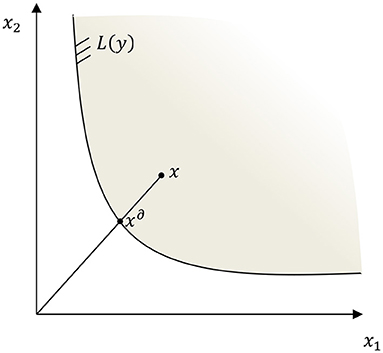
Figure 1. Input distance function.

D^I(x, y) can be interpreted as a multi-output input-requirement function allowing for deviations (distance) from the frontier. The input distance function is greater than or equal to one if the input vector is an element of the feasible set, L(y). The distance function is equal to unity if x is located on the boundary of the input set. D^I(x, y) is assumed to be non-decreasing, positively linearly homogenous and concave in inputs and non-increasing in outputs (Kumbhakar et al., 2008). Thus, all the deviations from the frontier are interpreted in terms of technical efficiency, TE. The input-contracting view of technical efficiency leads to the following definition:

$\begin{array}{ll}T{E}^I\left(x,y\right)={\left[D^I\left(x,y\right)\right]}^{-1}& (3)\end{array}$

This measure assumes values in the interval (0, 1] and the points for which D^I(x, y) = 1 define the boundary of the input requirement set. TE^I(x, y) can be interpreted as the proportion of the observed inputs that could be used to produce the same amount of output (Kumbhakar and Lovell, 2003, p. 50). By definition, the input distance function is linearly homogeneous in inputs, i.e., D^I(wx, y) = wD^I(x, y) for any w > 0. Linear homogeneity can be imposed by normalizing all inputs by the value of a normalizing input:, by setting w to $\frac{1}{x_1}$ we obtain $D^I\left(x,y\right)/x_1=D^I\left(\frac{x}{x_1},y\right)=D^I\left(x^{*},y\right)$, where $x^{*}=\frac{x}{x_1}$. This normalization is also necessary for estimation of the parameters of the distance function as it turns the implicit function in Equation (2) into a function with dependent and independent variables.

Suppose that we have data on inputs and outputs for a sample of farms. Then, for producer i we get:

$\begin{array}{ll}T{E}_i^I={\left[D^I\left(x_i,y_i\right)\right]}^{-1}{e}^{-v_i}\iff ln{D}^I\left(x_i,y_i\right)=lnT{E}_i^I+v_i& (4)\end{array}$

where v_i is a white-noise error term. From the above homogeneity property, we have:

$\begin{array}{l}ln{D}^I\left(x_i,y_i\right)=ln{D}^I\left(x_i^{*},y_i\right)+ln{x}_1\iff -ln{x}_1=ln\\ D^I\left(x_i^{*},y_i\right)-ln{D}^I\left(x_i,y_i\right)& (5)\end{array}$

with $x_i^{*}=\frac{x_i}{x_1}$ and x₁ being the normalizing input. Substituting (4) in (5) leads to an estimable form of the input distance function:

$\begin{array}{l}-ln{x}_1=ln{D}^I\left(x_i^{*},y_i\right)+lnT{E}_i^I+v_i=ln{D}^I\left(x_i^{*},y_i\right)\\ -u_i^I+v_i& (6)\end{array}$

where $u_i^I=-lnT{E}_i^I$ is treated as an one-sided error term. Abstracting from the context of a distance function, Equation (6) constitutes a typical representation of a stochastic frontier model (Aigner et al., 1977; Meeusen and van den Broeck, 1977) and the equation can be estimated econometrically using maximum likelihood techniques, assuming that v_i is independently and identically distributed random variable, $N\left(0,{\sigma }_v^2\right)$.

As output crop composition influences both the production frontier and the efficiency with which producers utilize resources, a modified non-neutral approach developed by Huang and Liu (1994) has to be employed. In reality, technical efficiency is dependent on the input choices and the method of application of inputs. Some vegetables may need more inputs and require more management skills than other vegetables. Following Alvarez et al. (2006) and Dinar et al. (2007), $u_i^I$ is modeled as:

$\begin{array}{ll}{u}_i^I=g\left(z_i;\delta \right)+{\epsilon }_i,& (7)\end{array}$

where z is a vector of explanatory variables which includes an output specialization index, interactions between this index and the elements of x_i, and farm-specific characteristics (e.g., demographic, socio-economic, etc.) (Huang and Liu, 1994; Dinar et al., 2007); δ is a vector of parameters to be estimated and ε is a random error referring to the unexplained or residual technical efficiency. The requirement that $u_i^I=g\left(z_i;\delta \right)+{\epsilon }_i\ge 0$ is met by truncating ε_i from below such that ε_i ≥ −g(z_i; δ), and ε_i is assumed to be an independently, but not identically distributed random variable with ${\epsilon }_i~N\left(0,{\sigma }_{\epsilon }^2\right)$.¹ Substituting Equation (7) into Equation (6) yields:

$\begin{array}{ll}-ln{x}_1=ln{D}^I\left(x_i^{*},y_i\right)+v_i-\left[g\left(z_i;\delta \right)+{\epsilon }_i\right],& (8)\end{array}$

The assumptions imposed on $u_i^I$ and ε_i are consistent with $u_i^I~N^{+}\left(g\left(z_i;\delta \right),{\sigma }_u^2\right)$ (Battese and Coelli, 1995), and that v_i and $u_i^I$ are distributed independently (Kumbhakar and Lovell, 2003, p. 267). The first term on the right-hand side of Equation (8) is the composition in the frontier quantity of inputs as well as the spatial heterogeneity; the g(·) function gives the heterogeneity in the distance to the frontier, i.e., technical efficiency. The information contained in the first right-hand side term can be used to test whether economies of scope exist.

A few comments are in place here. First, our production frontier estimation in (8) yields two effects of crop specialization on input use. The first partial derivative of the input distance function defined in (8) with respect to an output is assumed to be negative, implying that an extra unit of output ceteris paribus reduces the amount by which the input vector has to be deflated to reach the production frontier (Coelli and Fleming, 2004). The dual relation between the cost function and the input distance function can be exploited to derive a measure of economies of scope (or cost complementarities) without requiring estimates of the parameters of the cost function (Hajargasht et al., 2008; Nemoto and Furusmatsu, 2014; Färe and Karagiannis, 2018). This approach has the advantage that the estimation can proceed using only the input distance function and without requiring input price data, which are not available in our case (especially for capital and land).

Second, our non-neutral specification gives a marginal contribution of output specialization on technical efficiency and varies with the farm's input utilization. It is important to indicate that our model is different from the one used by Rahman (2009) to explain the effect of diversification on technical efficiency. Rahman assumed a neutral specification where the marginal effect of crop diversification on technical efficiency is constant. Furthermore, our model specification is different from the one used by Hajargasht et al. (2008) because in our specification we account for the effect of additional explanatory variables on technical efficiency. Färe and Karagiannis (2018) follows the approach of Hajargasht et al. (2008) but their primal production technology is modeled by a directional rather than a radial distance function by defining a direction function. However, we use the algorithm described by Hajargasht et al. (2008) to compute a measure of economies of scope. Since the Huang and Liu (1994) paper, in which a neutral specification is demonstrated to suffer from misspecification, the non-neutral stochastic frontier model is preferred to a neutral model in many empirical applications (Alvarez et al., 2006; Dinar et al., 2007; Karagiannis and Tzouvelekas, 2009). These authors argued that the conventional formulation and estimation of the stochastic frontier production function may not be appropriate in identifying the sources of technical inefficiency in production. Also, Dinar et al. (2007) have shown that the hypothesis of a neutral shift in the production frontier is strongly rejected. Paradoxically, estimation of the non-neutral specification is still the exception rather than the norm in the literature.

For the empirical implementation, we approximate the input distance function by a Translog form. The Translog is a flexible functional form which approximates any twice differentiable function without imposing a priori restrictions on the production technology. In the case of a distance function, Kumbhakar and Lovell (2003, p. 94) also indicated that the Translog is the appropriate functional form over the Cobb-Douglas.

However, a complication arises with the “traditional” Translog specification because some producers in the sample are perfectly specialized in one category of vegetables (i.e., traditional or non-traditional vegetables). For this reason a modified Translog function is used in which vegetable outputs are adjusted according to the Battese (1997) transformation (see Tsekouras et al., 2004). Moreover, variables related to soil fertility are included in the production frontier model to account for spatial heterogeneity (see e.g., Sherlund et al., 2002; Dinar et al., 2007; Okoror and Areal, 2020). In the same line, other studies like Skevas and Oude Lansink (2020) and Pede et al. (2018) among others investigate the role of spatial dependency in the technical efficiency estimates by using georeferenced coordinates to account for spatial heterogeneity. The empirical model is given by:

$\begin{array}{l}ln\frac{D_i^I}{x_{1,i}}={\beta }_0+{\displaystyle \sum _d^D}{\beta }_d{F}_{di}+{\beta }_1{D}_{1i}+{\beta }_2{D}_{2i}+{\displaystyle \sum _k^K}{\beta }_{k^{*}}ln{x}_{ki}^{*}+\frac{1}{2}\\ {\displaystyle \sum _k^K}{\displaystyle \sum _l^K}{\beta }_{k^{*}{l}^{*}}ln{x}_{ki}^{*}ln{x}_{li}^{*}+{\displaystyle \sum _m^M}{\beta }_{m}ln{y}_{mi}\\ +\frac{1}{2}{\displaystyle \sum _m^M}{\displaystyle \sum _n^M}{\beta }_{mn}ln{y}_{mi}ln{y}_{ni}+\frac{1}{2}{\displaystyle \sum _k^K}{\displaystyle \sum _m^M}{\beta }_{km}ln{x}_{ki}^{*}ln{y}_{ni}& (9)\end{array}$

where x^*s are input quantities normalized by x₁, ys are output quantities, Fs are physical soil production characteristics, and i indexes farms. D₁ is a dummy variable for traditional vegetable production with D₁ = 1 if y_Trad = 0 and D₁ = 0 if y_Trad > 0; and y₁ = Max(y_Trad, D₁). Similarly, D₂ is a dummy variable for non-traditional vegetable production with D₂ = 1 if y_NTrad = 0 and D₂ = 0 if y_NTrad > 0; and y₂ = Max(y_NTrad, D₂). Using (8), we obtain the following estimable form:

$\begin{array}{l}-ln{x}_{1,i}={\beta }_0+{\displaystyle \sum _d^D}{\beta }_d{F}_{di}+{\beta }_1{D}_{1i}+{\beta }_2{D}_{2i}+{\displaystyle \sum _k^K}{\beta }_{k^{*}}ln{x}_{ki}^{*}+\frac{1}{2}\\ {\displaystyle \sum _k^K}{\displaystyle \sum _l^K}{\beta }_{k^{*}{l}^{*}}ln{x}_{ki}^{*}ln{x}_{li}^{*}+{\displaystyle \sum _m^M}{\beta }_{m}ln{y}_{mi}\\ +\frac{1}{2}{\displaystyle \sum _m^M}{\displaystyle \sum _n^M}{\beta }_{mn}ln{y}_{mi}ln{y}_{ni}+\frac{1}{2}{\displaystyle \sum _k^K}{\displaystyle \sum _m^K}{\beta }_{km}ln{x}_{ki}^{*}ln{y}_{ni}-u_i^I+v_i& (\mathrm{10a})\end{array}$

The modified non-neutral efficiency part of the model with interactions is given by:

$\begin{array}{ll}{u}_i^I={\delta }_0+{\delta }_{I}Sp{e}_i+{\displaystyle \sum _k^K}{\delta }_{Ik}Sp{e}_{i}ln{x}_{ki}^{*}+{\displaystyle \sum _j^J}{\delta }_{Ij}Sp{e}_i{A}_{ji}+{\epsilon }_i& (\mathrm{10b})\end{array}$

Spe refers to specialization index and As are farm characteristics; x^*s are the same as defined in (9).

Economies of Scale and Economies of Scope

Since the input distance function is homogeneous of degree one in inputs, from equation (10a), the input elasticity for output y_m, $-{\epsilon }_{D^I,y_m}=-\frac{\partial ln{D}^I}{\partial ln{y}_m}=\frac{\partial ln{x}_1}{\partial ln{y}_m}={\epsilon }_{x,y_m}$, represents the percent change in x₁ from a 1% change in y_m, holding all input ratios x^* (and thus input composition) constant. The scale elasticity can be calculated as the negative sum of the input-output elasticities; that is, $-{\epsilon }_{D^I,y}=-\sum _1^M\frac{\partial ln{D}^I}{\partial ln{y}_m}=\sum _1^M\frac{\partial ln{x}_1}{\partial ln{y}_m}=\sum _1^M{\epsilon }_{x,y_m}={\epsilon }_{x,y}$. The measure of scale economies is indicated by the short-fall of ε_{X, Y} from unity.

In a multiproduct production technology, economies of scope exist when, for outputs y₁ and y₂, the average cost of joint production is less than the cost of producing each output separately (Teece, 1980; Panzar and Willig, 1981; Cowing and Holtmann, 1983). That is, economies of scope are defined as:

$\begin{array}{ll}EOS=C\left(y_1,0\right)+C\left(0,y_2\right)-C\left(y_1,y_2\right)& (11)\end{array}$

where C(y₁, y₂) is the cost of producing both outputs simultaneously and C(y₁, 0) and C(0, y₂) denote the cost of producing the two outputs separately. Economies of scope exist if EOS > 0, in which case the cost of producing the outputs separately is higher than the cost of producing them jointly.

More generally, a sufficient condition for the presence of economies of scope between outputs m and n is:

$\begin{array}{ll}\frac{{\partial }^{2}C\left(·\right)}{\partial y_m\partial y_n}<0,\text{for }m\ne n& (12)\end{array}$

where C(·) is the variable cost function. This expression implies that the cost function exhibits cost complementarities.

The input distance function and the cost function are dual to one another, meaning that the information contained in the input distance function about the production technology is identical to the cost function (Färe and Primont, 1995, p. 47–48). In this study, economies of scope are measured using a primal input distance function. Consequently, we use the dual measure of economies of scope approach developed by Hajargasht et al. (2008) and extended by Färe and Karagiannis (2018). In this paper, the derivative-based measure of economies of scope is obtained by exploiting the duality between the shadow cost function and the input distance function. Focusing on the sufficient condition in (13), by Hajargasht et al. (2008) derived a general expression to calculate the economies of scope between outputs i and j using the derivatives of the input distance function as follows:

$\begin{array}{ll}{C}_{yy}=C\left\{D_y^I{D}_y^{I^{\prime }}-D_{yy}^I+D_{yx}^I{\left[D_{xx}^I+D_x^I{D}_x^{I^{\prime }}\right]}^{-1}{D}_{xy}^I\right\}& (13)\end{array}$

where subscripts denote partial differentiation.

From this equation, one can find that information on the sign of the second cross partial derivatives of outputs, $D_{yy}^I\left(m,n\right)$, is not sufficient to conclude if scope economies exist or not. As shown by Hajargasht et al. (2008), if the technology satisfies certain restrictions, such as input homotheticity or global constant returns to scale, simpler expressions are obtained. A value of (14) less than zero (i.e., $\frac{C_{yy}}{C}<0$) indicates the presence of economies of scope, meaning that a vegetable producer has an incentive to diversify. In contrast, a value greater than zero (i.e., $\frac{C_{yy}}{C}>0$) represents diseconomies of scope, implying that a producer has an incentive to specialize in the production of one output category. Following Hajargasht et al. (2006), if all inputs are scaled prior to estimating the input Translog distance function so that their means are equal to one, then the log of these means are equal to zero. Hence, the first derivatives are:

$\begin{array}{ll}\frac{\partial D}{\partial x_m}={\beta }_k\text{ and }\frac{\partial D}{\partial y_m}={\beta }_m& (14)\end{array}$

and the second derivatives become:

$\begin{array}{l}\frac{{\partial }^{2}D}{\partial x_k^2}={\beta }_k^2-{\beta }_k+{\beta }_{kk},\frac{{\partial }^{2}D}{\partial x_k\partial x_l}={\beta }_k{\beta }_l+{\beta }_{kl}\text{ and }\frac{{\partial }^{2}D}{\partial x_k\partial y_m}\\ ={\beta }_k{\beta }_m+{\beta }_{km}& (15)\end{array}$

The matrix of scope measures is:

$\begin{array}{l}\left[\begin{array}{ccc}{\beta }_1-{\beta }_{11}& \cdots & {\beta }_{1m}\\ ⋮& \ddots & ⋮\\ -{\beta }_{m1}& \cdots & {\beta }_m-{\beta }_{mm}\\ \end{array}\right]+\left[\begin{array}{ccc}{\beta }_1{\beta }_1& \cdots & {\beta }_k{\beta }_1+{\beta }_{k1}\\ ⋮& \ddots & ⋮\\ {\beta }_1{\beta }_m+{\beta }_{1m}& \cdots & {\beta }_k{\beta }_m+{\beta }_{km}\\ \end{array}\right]\\ {\left[\begin{array}{ccc}2{\beta }_1^2+{\beta }_{11}-{\beta }_1& \cdots & 2{\beta }_1{\beta }_k+{\beta }_{1k}\\ ⋮& \ddots & ⋮\\ 2{\beta }_k{\beta }_1+{\beta }_{k1}& \cdots & 2{\beta }_k^2+{\beta }_{1k}-{\beta }_k\\ \end{array}\right]}^{-1}\\ \left[\begin{array}{ccc}{\beta }_1{\beta }_1+{\beta }_{11}& \cdots & {\beta }_1{\beta }_m+{\beta }_{1m}\\ ⋮& \ddots & ⋮\\ {\beta }_k{\beta }_1+{\beta }_{k1}& \cdots & {\beta }_k{\beta }_m+{\beta }_{km}\\ \end{array}\right]& (16)\end{array}$

Those formulas are used to estimate the economies of scope of vegetable producers.

Data and Specification of the Model Variables

Data used in this study are part of a broader survey on the structural characteristics of the vegetable sector in southern Benin. The survey is based on farm-level cross-section data for the agricultural year 2009/2010. A multistage stratified random sampling technique was employed to locate the departments, the districts in each of the four departments, and the sample households. The sample vegetable producers were selected based on the information on the total number of vegetable producers including their farms size categories, which were obtained from a census survey in each district. Relative to the importance of vegetable production statistics from the Ministry of Agricultural of Benin, two districts out of six were selected in the department of Mono, two out of nine in the department of Oueme, one out of eight in the department of Altantique and one out one in the department of Littoral. In the department of Mono, the districts of Agoue and Grand-Popo were selected; the districts of Porto-Novo and Seme-Kpodji in the department of Oueme, the district of Ouidah in the department of Atlantique and the district of Cotonou in the department of Littoral. The census survey data gave a total of 1,247 vegetable producers in the six districts with 217 in Agoue, 149 in Grand-Popo, 115 in Porto-Novo, 77 in Seme-Kpodji, 92 in Ouidah and 597 in Cotonou. Then a stratified random sampling procedure was applied using a formula from Whitley and Ball (2002) with a 5% error limit. The target sample size of 25% of the total number of vegetable producers was then applied in each selected district. Hence, data were collected from 310 vegetable producers. Finally, 239 vegetable producers for which data were available for all variables were retained in this study. The 71 vegetable producers were dropped because there was no harvest information, they had cultivated other crops than vegetables like maize or there was inconsistent information. Vegetable producers are usually involved in producing two categories of vegetables, i.e., traditional and non-traditional vegetables. The data set contains 23 non-traditional (y_NTrad) vegetable crops and 10 traditional (y_Trad) vegetable crops (see Achigan-Dako et al., 2009 for details on grouping).² Four inputs are distinguished: cost of materials (x_Mat) that include fertilizer, pesticides, seeds, and other miscellaneous expenses; farm labor in hours (x_Lab); capital (x_Cap) measured in replacement cost and farmland in hectares (x_Land). Two soil fertility indicators (dummy) variables are used as additional variables in the specification of the distance function to account for spatial heterogeneity of vegetables production. High soil fertility is expected to lead, ceteris paribus, to lower input requirements for the production of a given amount output and, thus, have a positive effect on the value of the input distance function. We define three dummies variable for soil fertility namely best, medium, and low to control for farm space heterogeneity. We set low soil fertility variable as a reference and include the remaining two soil fertility dummies in the estimations.

The specialization variable is specified as a normalized Hirschman index of the concentration of output shares for each vegetable crop. This index discriminates between producers who are relatively more specialized. It is a widely used measure of concentration and was used, for example, by Al-Marhubi (2000) to specify the concentration of output shares in his analysis of export diversification and growth. Following Al-Marhubi (2000, p. 561), the normalized Hirschmann index is defined as follows:

$\begin{array}{ll}{H}_i=\frac{\sqrt{{\displaystyle {\sum }_j^{33}}{\left(\frac{q_j}{{\displaystyle {\sum }_j^{33}}{q}_j}\right)}^2}-\sqrt{\frac{1}{33}}}{1-\sqrt{\frac{1}{33}}}& (17)\end{array}$

where i is the producer index, q_j represents the producer output quantity of vegetable crop j, and 33 is the number of vegetables produced, as they are recorded in the data set. The Hirschmann index is normalized to assume values ranging from 0 to 1. Note that a normalized Hirschmann index of 1 indicates perfect specialization. Likewise, a value closer to 0 signifies a more diversified vegetable crop production.

Based on the existing literature, farmers' socio-economic characteristics are included in the model. These are: producers' education (EDUC), and farming experience (EXP), both measured in years. Most empirical studies found that farm experience and producer education have the strongest impact on the producer management practices. For example, Pope and Prescott (1980) found that less experienced farmers (or younger farmers) are more specialized as they may start small and specialized operations, and perhaps become more diversified as they expand their operations. Katchova (2005) found that more educated farmers have higher excess farm values. The ratios of the amount of credit received by a producer over total revenue (MCRED), and the proportion of vegetables sold to the wholesaler (WHOLE) are included to represent socioeconomic characteristics of farms. Vegetable cultivation requires more purchased inputs such as fertilizers, pesticides, and irrigation water, increasing the need for liquidity. Vegetable cultivation also demands more labor than field crops, such as cereals and a large proportion of labor in vegetable cultivation is hired labor (Ali and Abedullah, 2002). All these conditions increase the demand for liquidity in vegetable production. Consequently, more loans are required to finance vegetable production. Vegetables have a shorter shelf life than cereal crops, so strong relationships between producers and buyers are essential to ensure a timely delivery to the market. Hence, the proportion of vegetable output sold to wholesalers is included in the model as an explanatory variable. Table 1 presents summary statistics for all farms. Aggregate non-traditional vegetable outputs represent 55% of the total vegetable output share, meaning that producing non-traditional vegetables is one of the strategic decisions made by producers.

TABLE 1

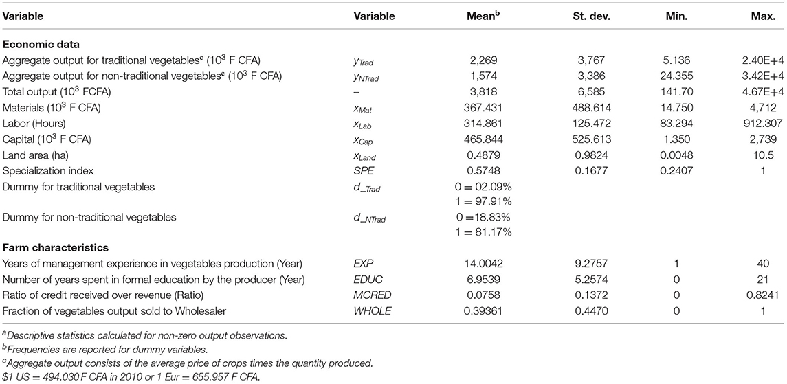
Table 1. Descriptive statistics of the variables^a (n = 239).

In our model specification in equation (10a), capital is set as the normalizing input x₁ so that all other inputs are represented relative to capital. All input and output variables are mean-corrected prior to estimation, so that the coefficients of the first-order terms can be directly interpreted as distance elasticities evaluated at the geometric mean of the data. That is, each output and input variable has been divided by its geometric mean.

Empirical Results

Economies of Scale and Economies of Scope

The model is estimated using Bayesian methods and Markov chain Monte Carlo (MCMC) techniques. The data are processed in R, and sampling from the posterior distribution of the parameters was performed in WinBUGS, which was called from R's “R2WinBUGS” interface. We also make use of a Bayesian econometrics software (BayES) which is a software designed for performing Bayesian inference using MCMC techniques to estimate the stochastic frontier models (Emvalomatis, 2020). We place vague priors on all parameters in the model. In particular, we use Normal priors for the parameters associated with independent variables, either in the frontier or in the specification of the technical efficiency terms, and Gamma (0.001; 0.001) priors for the inverses of the variance parameters. Estimation involves 100,000 iterations, with a burn-in period of 20,000 iterations. Posterior means and standard deviations of the parameters of the Translog specification of the input distance function based upon the remaining 80,000 iterations are reported in Table 2. Out of the 25 estimates, 15 had standard deviations that are small relative to theirs means, indicating that, overall, the model is well-specified. The results show that the absolute value of all elasticities (first-order terms for input and output variables) are between zero and one and possess the expected signs at the geometric mean. Hence, the input distance function satisfies the property of monotonicity, i.e., the input distance function is non-decreasing in inputs and non-increasing in outputs.

TABLE 2

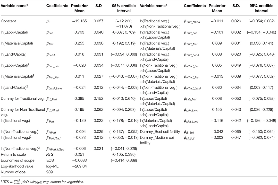
Table 2. Bayesian MCMC estimates of the Translog input distance function frontier.

The fact that the first-order terms for inputs are positive indicates that extra input increases the distance to the frontier, ceteris paribus and the negative first-order terms for outputs means that extra output decreases the distance to the frontier, ceteris paribus. Returns to scale at the geometric mean of the data is calculated as the negative of the sum of the first-order output coefficients and has a mean of 0.14, with a 95% credible interval of (0.04; 0.25). The result of returns to scale indicates possible presence of increasing returns to scale at the sample mean. The null hypothesis of constant returns to scale (CRS) is then rejected. Additionally, the inverse of this sum is equal to 7.14, providing a measure of Ray scale economies, suggesting the presence of increasing returns to scale. Thus, the transformation process described in our model may be thought of as exhibiting increasing returns to scale. This finding is consistent with results in many other empirical analyses of small-scale farms (e.g., Coelli and Fleming, 2004) and implies that vegetable farms are likely to benefit from scale increases. The individual output contributions underlying the scale elasticity show that both categories of output contributed significantly to input use. The result indicates that traditional vegetables require a greater input share than non-traditional vegetables. However, both outputs appear to have almost similar output share (45% for traditional vegetables and 55% for non-traditional vegetables) (Table 1). This result is important for computing the economies of scope in the next paragraph as the calculation of economies of scope are based on an input distance function that exhibits variable returns to scale. The Pearson correlation test indicates that the two outputs are not correlated. However, the theory of diversification points out that even though a Pearson correlation test shows that two outputs are not correlated, the production of one can be reduced if uncertainty over the second output rises (Just and Pope, 1978).

To further investigate the implications of our estimates about output complementarities, we now focus on the economies of scope, as presented in equation (16). Since the data are mean-corrected prior to the estimation of the distance function, the presence of economies of scope is evaluated at the geometric means of the sample data. The expression of $\frac{C_{yy}\left(1,2\right)}{C}$ evaluated at the sample means of the data is equal to −0.038 with a standard deviation of 5.17 and 95% credible interval of (−0.23; 0.18). Since the credible interval includes zero, we conclude that it is possible that there are neither positive nor negative EOS. As indicated above, a value of zero shows the absence of any cost gain in diversification whereas a value less than zero would mean a cost gain. The EOS value implies that there is no significant difference in terms of cost savings in producing both categories of vegetables or specializing in only one. In order words, the result shows no economic performance difference between specialized and diversified vegetable producers. Therefore, vegetable producers have no incentive for specialization or diversification in the production of one of the two outputs categories defined in this study.

Although a positive effect of soil fertility on the value of the distance function was expected, both parameters associated with the dummy variables associated with high and medium fertility were negative, on average, but their 95% credible intervals contain zero. Thus, soil fertility was not found to have an impact on the input requirements set and this could be due to farmers adjusting both the types of vegetables they are producing, as well as the proportions at which they are using inputs to counterbalance the effects of low soil fertility. More detailed fertility indexes, specific to the requirements of each vegetable could produce different results.

Impact of Specialization on Technical Efficiency

Table 3 provides the posterior means, the standard deviations of the parameters and the 95% credible intervals for the non-neutral technical efficiency effects.

TABLE 3

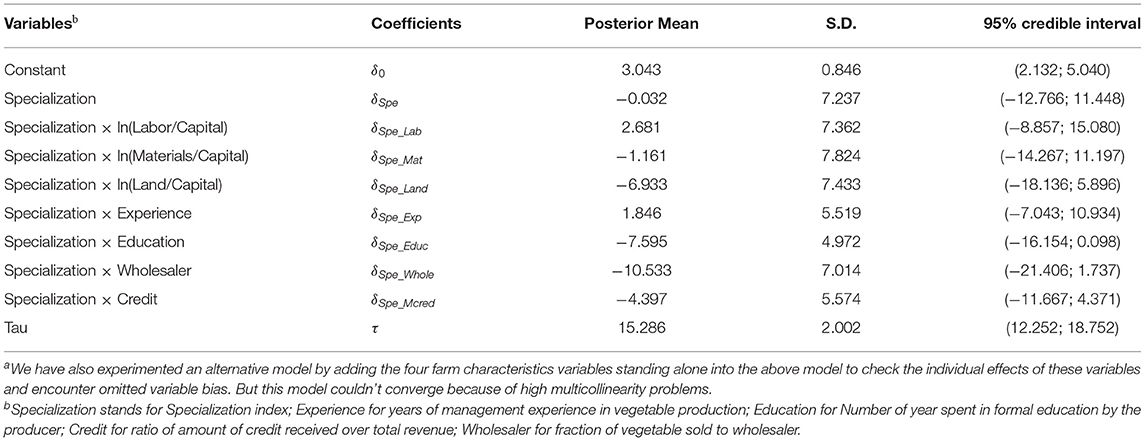
Table 3. Bayesian estimates of the efficiency effect model (non-neutral specification).^a

Row 2 of Table 4 shows the average technical efficiency and its variation. The result reveals a positive skewness in the distribution of technical efficiency. The average technical efficiency of the sample is 94.27%, implying that the same output can be produced with 94% of the observed inputs. In addition, Table 4 reports the marginal effects of crop specialization on the technical efficiency, computed using (10b). The results suggest a positive effect of specialization on technical efficiency. This result seems to corroborate the decreasing technical efficiency of most diversified farms. As indicated by Wang (2002), the opposite marginal effects in these two quartiles show that specialization in vegetable outputs production affects technical efficiency non-monotonically in the sample. Consequently, the results cannot tell more about when the impact of crop specialization turns from negative to positive. Since we cannot interpret directly the meaning of the marginal effects, we also compute the elasticity of technical efficiency with respect to specialization. On average, the contribution of vegetable output specialization to technical efficiency is found to be low, but different from zero. Specifically, the result shows that a 1% increase in specialization is associated with a 0.79% increase in technical efficiency. The result implies that, on average, specialization generates gains in technical efficiency. This suggests that the costs of diversifying outweigh the benefits, and specializing is the preferred strategy, at least from a technical efficiency perspective and ignoring the risk-reducing effect of diversification. The results are consistent with the findings of many empirical works, indicating that diversification often requires specialized equipment and that diversified farms accumulate fewer assets than specialized farms (Harwood et al., 1999). In line with Katchova (2005), the results suggest that diversified vegetable farms had a lower excess value than specialized farms. The results are also in line with the finding of Llewelyn and Williams (1996) for irrigated farms in Indonesia, that greater diversification is associated with lower technical efficiency. Since vegetables are cash crops, the result stresses that diversification decreases technical efficiency. The reason for our finding is that the two categories of vegetables are grown in the same period and compete for the same inputs (labor, pesticides, fertilizers and water) and require similar managerial skills. Like in Rahman (2009) study of smallholders in Bangladesh, the worsening evidence of diversification economies observed between traditional and non-traditional vegetables is largely due to the practice of producing both categories of crops. From the survey results, it turns out that vegetable production is generally input intensive regardless of the type of vegetable considered. However, this result is in contrast with Coelli and Fleming (2004) who found that greater specialization leads to lower technical efficiency. In our paper, the two outputs y₁ and y₂ are already group of outputs. Thus, if there are any periods in which a crop requires a lot of labor while another crop none, farmers can exploit that by diversifying only within y₁ and y₂.

TABLE 4

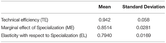
Table 4. Distribution of technical efficiency and the marginal effect and elasticity of technical efficiency with respect to specialization.

Conclusion and Policy Implications

This paper provides an empirical evaluation of the impact of crop specialization on vegetable producers' economic performance in Benin. The challenge in this study was to assess whether changes in farm orientation through diversification or specialization can be attributed to the search for greater economic performance, while also controlling for spatial heterogeneity. We based our estimation on a non-neutral stochastic frontier model to test and consider the adjustment of input utilization with output choices and estimate the effect of specialization on the production technology and performance. Duality theory is used to obtain a measure of economies of scope without requiring the econometric estimation of a cost function. The article employs a parametric method in estimating an input distance function using a modified Translog specification and a truncated efficiency regression, representing efficiency in production. The results show a prevalence of increasing returns to scale. The results also provide evidence for the absence of economies of scope, indicating that vegetable producers have a relative low incentive for specialization in either traditional or non-traditional vegetables.

The contribution of vegetable output specialization to technical efficiency is found to be quite low, but significant. Specifically, a 1% increase in crop specialization is associated with a 0.79% increase in technical efficiency.

Although soil quality is important condition, the results show that farmers are adjusting the proportions at which they are using manure and inorganic fertilizers to counterbalance the effects of low soil fertility. Since soil types are obtained from farmers' perception, we recommend further research where and appropriate soil test be carried out rather than relying on the perception of the farmers as indicated by Okoror and Areal (2020).

A limitation of this study is that, although we observe farmers producing 33 crops, we aggregate them into two types of outputs (traditional and non-traditional). This was done due to the number of parameters that need to be estimated growing at an exponential level in the number of output categories. However, with more data points one could consider more detailed classifications of output, for example leafy vegetables, fruits, roots and tubers.

Our results suggest that policy makers aiming at food security and agricultural growth may also enhance specialization. The policy implication of this paper is that agricultural policy might also encourage specialization in high value-added products like non-traditional vegetables.

Data Availability Statement

The original contributions presented in the study are included in the article/Supplementary Material, further inquiries can be directed to the corresponding author/s.

Author Contributions

AS: conceptualization, methodology, software, validation, formal analysis, data curation, writing–original draft, and writing–review and editing. GE: methodology, software calibration, and writing–reviewing. AO: methodology, writing–original draft, and validation. All authors contributed to the article and approved the submitted version.

Conflict of Interest

The authors declare that the research was conducted in the absence of any commercial or financial relationships that could be construed as a potential conflict of interest.

Publisher's Note

All claims expressed in this article are solely those of the authors and do not necessarily represent those of their affiliated organizations, or those of the publisher, the editors and the reviewers. Any product that may be evaluated in this article, or claim that may be made by its manufacturer, is not guaranteed or endorsed by the publisher.

Acknowledgments

The authors would like to thank two referees and the editor for their comments that substantially improved this paper. We are also grateful for the financial support that was provided for this study by the Dutch government scholarship through the Netherlands fellowship programs. The fieldwork was facilitated by the excellent support of the National Institute of Agricultural Research of Benin (INRAB) and enumerators.

Supplementary Material

The Supplementary Material for this article can be found online at: https://www.frontiersin.org/articles/10.3389/fsufs.2021.711530/full#supplementary-material

Footnotes

1. ^In the spirit of Huang and Liu (1994), ε_i is assumed to follow a normal distribution with zero mode, truncated from below at a variable truncation point [−g(z_i; δ)], which allows ε_i ≤ 0, but enforces $u_i^I$ ≥ 0.

2. ^The term non-traditional vegetable refers to species such as lettuce, cabbage, courgette, cucumber, beet, carrot, radish, turnip, french bean, melon, squash, watermelon, celery, chicory, chives, coriander, dill, fennel, garden mint, leek, overripe, parsley, rocket and thyme. Species such as tomato, solanum, okra, pepper, amaranth, corchorus, bitterleaf, african basil, cockscomb and onion are considered as traditional vegetables.

References

Achigan-Dako, E. G., Pasquini, M. W., and Assogba Komlan, F. (2009). “Inventory and use of traditional vegetables: methodological framework,” in Traditional Vegetables in Benin: Diversity, Distribution, Ecology, Agronomy, and Utilization, eds Achigan-Dako et al., Bangor: Darwin Initiative, 9–51.

Aigner, D. J., Lovell, C. A. K., and Schmidt, P. (1977). Formulation and estimation of stochastic frontier production function models. J. Econom. 6, 21–37. doi: 10.1016/0304-4076(77)90052-5

CrossRef Full Text | Google Scholar

Akinola, A. A., and Eresama, P. C. (2009). Economics of amaranthus production under tropical conditions. Int. J. Veg. Sci. 16, 32–43. doi: 10.1080/19315260903178655

CrossRef Full Text | Google Scholar

Ali, M. (2008). “Horticulture revolution for the poor: nature, challenges and opportunities.” in Background Paper 41353 (Shanhua; Tainan: AVRDC-The World Vegetable Center), 40.

Google Scholar

Ali, M., and Abedullah, D. (2002). Nutritional and economic benefits of enhanced vegetable production and consumption. J. Crop Prod. 6, 145–176. doi: 10.1300/J144v06n01_09

CrossRef Full Text | Google Scholar

Al-Marhubi, F. (2000). Export diversification and growth: an empirical investigation. Appl. Econ. Lett. 7, 559–562. doi: 10.1080/13504850050059005

CrossRef Full Text | Google Scholar

Alvarez, A., Amsler, C., Orea, L., and Schmidt, P. (2006). Interpreting and testing the scaling property in models where inefficiency depends on firm characteristics. J. Prod. Anal. 25, 201–212. doi: 10.1007/s11123-006-7639-3

CrossRef Full Text | Google Scholar

Battese, G. E. (1997). A note on the estimation of the Cobb-Douglas production function when some explanatory variables have zero values. J. Agric. Econ. 48, 250–252. doi: 10.1111/j.1477-9552.1997.tb01149.x

CrossRef Full Text | Google Scholar

Battese, G. E., and Coelli, T. J. (1995). A model for technical inefficiency effects in a stochastic frontier production function for panel data. Empir. Econ. 20, 325–332. doi: 10.1007/BF01205442

CrossRef Full Text | Google Scholar

Binswanger, H. P. (1986). Evaluating research system performance and targeting research in land-abundant areas of Sub-Saharan Africa. World Dev. 14, 469–475. doi: 10.1016/0305-750X(86)90063-X

CrossRef Full Text | Google Scholar

Byerlee, D., de Janvry, A., and Sadoulet, E. (2009). Agriculture for development: toward a new paradigm. Ann. Rev. Resour. Econ. 1, 15–31. doi: 10.1146/annurev.resource.050708.144239

CrossRef Full Text | Google Scholar

Chavas, J.-P. (2011). Agricultural policy in an uncertain world. Eur. Rev. Agric. Econ. 38, 383–407. doi: 10.1093/erae/jbr023

CrossRef Full Text | Google Scholar

Coelli, T., and Fleming, E. (2004). Diversification economies and specialization efficiencies in a mixed food and coffee smallholder farming system in Papua New Guinea. Agric. Econ. 31, 229–239. doi: 10.1111/j.1574-0862.2004.tb00260.x

CrossRef Full Text | Google Scholar

Coelli, T., and Perelman, S. (1996). “Efficiency measurement, multiple-output technologies and distance functions: with application to European railways,” in Working paper CREPP 96/05, Centre de Recherche en Economie Publique et en Economie de la Population (Belgium: Université de Liège), 31.

Google Scholar

Cowing, T. G., and Holtmann, A. G. (1983). Multiproduct short-run hospital cost functions: empirical evidence and policy implications from cross-section data. South. Econ. J. 49, 637–653. doi: 10.2307/1058706

CrossRef Full Text | Google Scholar

Dinar, A., Karagiannis, G., and Tzouvelekas, V. (2007). Evaluating the impact of agricultural extension on farms performance in Crete: a non-neutral stochastic frontier approach. Agric. Econ. 36, 133–144. doi: 10.1111/j.1574-0862.2007.00193.x

CrossRef Full Text | Google Scholar

Emvalomatis, G. (2020). Bayesian Econometrics Software (BayES). User's Guide. Available online at: https://bayeconsoft.com/html_documentation.html (accessed June 8, 2021).

Färe, R., and Karagiannis, G. (2018). Inferring scope economies from the input distance function. Econ. Lett. 172, 40–42. doi: 10.1016/j.econlet.2018.07.037

CrossRef Full Text | Google Scholar

Färe, R., and Primont, D. (1995). Multi-output and Duality: Theory and Applications. Boston: Kluwer Academic Publishers, 172.

Google Scholar

Feder, G., Just, R. E., and Zilberman, D. (1985). Adoption of agricultural innovations in developing countries: a survey. Econ. Dev. Cult. Change 33, 255–298. doi: 10.1086/451461

CrossRef Full Text | Google Scholar

Fuglie, K. O. (2008). Is a slowdown in agricultural productivity growth contributing to the rise in commodity prices? Agric. Econ. 39, 431–441. doi: 10.1111/j.1574-0862.2008.00349.x

CrossRef Full Text | Google Scholar

Hajargasht, G., Coelli, T., and Rao, D. S. P. (2006). “A dual measure of economies of scope,” in Working Paper Series 03/2006 (St. Lucia, OLD: School of Economics; Center for Efficiency and Productivity Analysis, University of Queensland).

Google Scholar

Hajargasht, G., Coelli, T., and Rao, D. S. P. (2008). A dual measure of economies of scope. Econ. Lett. 100, 185–188. doi: 10.1016/j.econlet.2008.01.004

CrossRef Full Text | Google Scholar

Haji, J. (2008). Economic Efficiency and Marketing Performance of Vegetable Production in the Eastern and Central Parts of Ethiopia (Doctoral thesis). Uppsala: Swedish University of Agricultural Sciences, 64.

Google Scholar

Harwood, J., Heifner, R., Coble, K., Perry, J., and Somwaru, A. (1999). Managing Risk in Farming: Concepts, Research, and Analysis. Washington, DC: Market and Trade Economics Division and Resource Economics Division, Economic Research Service, U.S. Department of Agriculture. Agricultural Economic Report No. 774, 125.

Google Scholar

Huang, C. J., and Liu, J.-T. (1994). Estimation of a non-neutral stochastic frontier production function. J. Prod. Anal. 5, 171–180. doi: 10.1007/BF01073853

CrossRef Full Text | Google Scholar

Jack, B. K. (2013). Constraints on the Adoption of Agricultural Technologies in Developing Countries. Literature review, Agricultural Technology Adoption Initiative, J-PAL (MIT) and CEGA (UC Berkeley). Berkeley, CA: California Digital Library; University of California.

Just, R. E., and Pope, R. D. (1978). Stochastic specification of production functions and economic implications. J. Econ. 7, 67–86. doi: 10.1016/0304-4076(78)90006-4

CrossRef Full Text | Google Scholar

Karagiannis, G., and Tzouvelekas, V. (2009). Measuring technical efficiency in the stochastic varying coefficient frontier model. Agric. Econ. 40, 389–396. doi: 10.1111/j.1574-0862.2009.00386.x

CrossRef Full Text | Google Scholar

Katchova, A. L. (2005). The farm diversification discount. Am. J. Agric. Econ. 87, 984–994. doi: 10.1111/j.1467-8276.2005.00782.x

CrossRef Full Text | Google Scholar

Keatinge, J. D. H., Yang, R.-Y., Hughes, J. d'A., Easdown, W. J., and Holmer, R. (2011). The importance of vegetables in ensuring both food and nutritional security in attainment of the Millennium Development Goals. Food Sec. 3, 491–501. doi: 10.1007/s12571-011-0150-3

CrossRef Full Text | Google Scholar

Kumbhakar, S. C., Lien, G., Flaten, O., and Tveteras, R. (2008). Impacts of Norwegian milk quotas on output growth: a modified distance function approach. J. Agric. Econ. 59, 350–369. doi: 10.1111/j.1477-9552.2008.00154.x

CrossRef Full Text | Google Scholar

Kumbhakar, S. C., and Lovell, K. C. A. (2003). Stochastic Frontier Analysis. Cambridge, UK: Cambridge University Press, 333.

Google Scholar

Llewelyn, R. V., and Williams, J. R. (1996). Nonparametric analysis of technical, pure technical, and scale efficiencies for food crop production in East Java, Indonesia. Agric. Econ. 15, 113–126. doi: 10.1111/j.1574-0862.1996.tb00425.x

CrossRef Full Text | Google Scholar

Meeusen, W., and van den Broeck, J. (1977). Efficiency estimation from Cobb-Douglas production functions with composed error. Int. Econ. Rev. 18, 435–444. doi: 10.2307/2525757

CrossRef Full Text | Google Scholar

Mekonnen, T. (2017). “Impact of agricultural technology adoption on market participation in the rural social network system,” in Working Paper Series #2017-008. Maastricht: United Nations University; Maastricht Economic and social Research institute on Innovation and Technology (UNU-MERIT); Maastricht University.

Google Scholar

Morrison-Paul, C. J. M., and Nehring, R. (2005). Product diversification, production systems, and economic performance in U.S. agricultural production. J. Econ. 126, 525–548. doi: 10.1016/j.jeconom.2004.05.012

CrossRef Full Text | Google Scholar

Nemoto, J., and Furusmatsu, N. (2014). Scale and scope economies of Japanese private universities revisited with an input distance function approach. J. Prod. Anal. 41, 213–226. doi: 10.1007/s11123-013-0378-3

CrossRef Full Text | Google Scholar

Okoror, O. T., and Areal, F. (2020). The effect of sustainable farming practices and soil factors on the technical efficiency of maize farmers in Kenya. Kasetsart J. Soc. Sci. 41, 641–646. doi: 10.34044/j.kjss.2020.41.3.29

CrossRef Full Text | Google Scholar

Oude Lansink, A., and Stefanou, S. (2001). Dynamic area allocation and economies of scale and scope. J. Agric. Econ. 52, 38–52. doi: 10.1111/j.1477-9552.2001.tb00937.x

CrossRef Full Text | Google Scholar

Panzar, J. C., and Willig, R. D. (1981). Economies of scope. Am. Econ. Rev. 71, 268–272.

Google Scholar

Pede, V. O., Areal, F. J., Singbo, A., McKinley, J., and Kajisa, K. (2018). Spatial dependency and technical efficiency: an application of a Bayesian stochastic frontier model to irrigated and rainfed rice farmers in Bohol, Philippines. Agric. Econ. 49, 301–312. doi: 10.1111/agec.12417

CrossRef Full Text | Google Scholar

Pope, R. D., and Prescott, R. (1980). Diversification in relation to farm size and other socioeconomic characteristics. Am. J. Agric. Econ. 62, 554–559. doi: 10.2307/1240214

CrossRef Full Text | Google Scholar

Rahman, S. (2009). Whether crop diversification is a desired strategy for agricultural growth in Bangladesh? Food Pol. 34, 340–349. doi: 10.1016/j.foodpol.2009.02.004

CrossRef Full Text | Google Scholar

Rahman, S., and Rahman, M. (2008). Impact of land fragmentation and resource ownership on productivity and efficiency: the case or rice producers in Bangladesh. Land Use Pol. 26, 95–103. doi: 10.1016/j.landusepol.2008.01.003

CrossRef Full Text | Google Scholar

Reimers, M., and Klasen, S. (2013). Revisiting the role of education for agricultural productivity. Am. J. Agric. Econ. 95, 131–152. doi: 10.1093/ajae/aas118

CrossRef Full Text | Google Scholar

Shephard, R. W. (1953). Cost and Production Functions. Princeton, NJ: Princeton University Press, 104.

Google Scholar

Shephard, R. W. (1970). The Theory of Cost and Production Functions. Princeton, NJ: Princeton University Press, 308.

Google Scholar

Sherlund, S. M., Barrett, C. B., and Adesina, A. A. (2002). Smallholder technical efficiency controlling for environmental production conditions. J. Dev. Econ. 69, 85–101. doi: 10.1016/S0304-3878(02)00054-8

CrossRef Full Text | Google Scholar

Skevas, I., and Oude Lansink, A. (2020). Dynamic inefficiency and spatial spillovers in Dutch dairy farming. J. Agric. Econ. 71, 742–759. doi: 10.1111/1477-9552.12369

CrossRef Full Text | Google Scholar

Teece, D. J. (1980). Economies of scope and the scope of the enterprise. J. Econ. Behav. Org. 1, 223–247. doi: 10.1016/0167-2681(80)90002-5

CrossRef Full Text | Google Scholar

Tsekouras, K. D., Pantzios, C. J., and Karagiannis, G. (2004). Malmquist productivity index estimation with zero-value variables: the case of Greek prefectural training councils. Int. J. Prod. Econ. 89, 95–106. doi: 10.1016/S0925-5273(03)00211-1

CrossRef Full Text | Google Scholar

Wang, H.-J. (2002). Heteroscedasticity and non-monotonic efficiency effects of a stochastic frontier model. J. Prod. Anal. 18, 241–253. doi: 10.1023/A:1020638827640

CrossRef Full Text | Google Scholar

Weinberger, K., and Lumpkin, T. A. (2007). Diversification into horticulture and poverty reduction: a research agenda. World Dev. 35, 1464–1480. doi: 10.1016/j.worlddev.2007.05.002

CrossRef Full Text | Google Scholar

Whitley, E., and Ball, J. (2002). Sample Size Calculations. Statistics Review 4. Available online at: http://ccforum.com/content/6/4/335 (accessed August 8, 2017).

PubMed Abstract