Evaluating the onset conditions of a thermoacoustic Stirling engine loaded with an audio loudspeaker

1 Introduction

Thermoacoustic engines convert heat into sound without any solid moving parts. They consist of an acoustic resonator enclosed by a porous medium, known as a stack or a regenerator, sandwiched between the hot and ambient heat exchangers. When the axial temperature gradient imposed on the porous medium exceeds the onset threshold, the spontaneous oscillation of gas undergoes thermodynamic cycles that convert externally supplied heat power to acoustic power, which can be transmitted to acoustic loads for various applications.

In particular, when the configuration involves a looped tube with a branch tube, the thermoacoustic engine can undergo a Stirling-like thermodynamic cycle with substantially high thermal efficiency. This is attributed to the establishment of high acoustic impedance and traveling wave phasing at the regenerator (Backhaus and Swift, 1999). Additionally, the absence of mechanical moving parts promises high reliability and low cost for thermoacoustic engines. Furthermore, the use of low-Prandtl-number inert gases as working fluids makes this technology environmentally friendly. Thermoacoustic engines inherit the benefits of external combustion engines, which are unlimited in the heat source they can use and should be considered a sustainable solution.

Thermoacoustic (-Stirling) engines have been reported as laboratory prototypes that exhibit substantially high thermal efficiency, achieving above 30% (Backhaus and Swift, 1999). For the broader implementation of thermoacoustic technology, experts have intensified efforts to develop thermoacoustic electricity generators. Various electrodynamic transduction mechanisms, such as the linear electrodynamic alternator (Gonen and Grossman, 2014; Bi et al., 2017), liquid column (Castrejón-Pita and Huelsz, 2007; Murti et al., 2023), and bi-directional turbine (Timmer and van der Meer, 2019; 2020), have been implemented. Recently, flywheel-crank-based mechanisms (Biwa et al., 2020; Penelet et al., 2021) using rotational alternators and liquid-metal-based triboelectric nanogenerators (Zhu et al., 2021) have been reported as acoustic loads for converting heat into electricity through thermoacoustic conversion.

The linear electrodynamic alternator has been reported to demonstrate the highest acoustic-to-electric conversion efficiency and power density among published studies (Timmer et al., 2018). In general, linear electrodynamic alternators have a very high mechanical impedance, which means that generating a small displacement requires a large force due to the use of “non-compliant” transducers comprising metal pistons (Yu et al., 2012). Placing the linear electrodynamic alternator in a high acoustic impedance region within the thermoacoustic engine is necessary for optimal operation at the resonant frequency of the combined system. However, the design of both the thermoacoustic engine and the linear electrodynamic alternator must be carefully and precisely considered (Timmer et al., 2018), as the high-impedance matching can restrict the flexibility of the engine’s configuration. Furthermore, the special design of the costly linear electrodynamic alternator can negate the advantage of the thermoacoustic engine’s low cost.

On the other hand, commercial audio loudspeakers are equipped with ultra-compliant transducers consisting of a light-moving coil and a fragile paper cone. Due to their relatively low impedance, loudspeakers are easy to drive and do not require strict conditions or criteria when being matched with thermoacoustic engines. Although loudspeakers have poor power transduction efficiency, their design emphasizes linearity (Marx et al., 2006) rather than efficiency conversion, making them highly suitable for building initial prototype configurations of thermoacoustic electric generators. Furthermore, commercially available loudspeakers are offered in a wide range of models, which aligns with the low-cost characteristics of thermoacoustic devices. Recently, Piccolo (2018) proposed a standing-wave-type low-cost thermoacoustic electricity generator that uses a commercial loudspeaker as a linear alternator, which has the advantage of a simpler design for the alternator–engine coupling and a more compact configuration. Furthermore, Chen et al. (2020) numerically investigated the coupling of thermoacoustic engines with external loads of varying stiffness coefficients, respectively, using the lumped element model and the (thermo-) acoustic network model. They suggested that ultra-compliant transducers provide better acoustic power extraction from thermoacoustic engines.

Numerous studies (Yu et al., 2012; Kang et al., 2015; Abdoulla-Latiwish et al., 2017; Abdoulla-Latiwish and Jaworski, 2019) have explored the coupling of commercial loudspeakers with thermoacoustic engines to leverage low-grade thermal energy. These studies have primarily concentrated on design methodologies aimed at enhancing performance metrics such as electrical power output or thermal-to-electric efficiency, with the majority being conducted using the well-known software package, Design Environment for Low-amplitude ThermoAcoustic Energy Conversion (DeltaEC) (Ward et al., 2012). Furthermore, Saha et al. (2012), utilizing 2D finite element method simulations, optimized and experimentally validated the superior performance of the double Halbach array structure over traditional loudspeakers specifically for thermoacoustic engines. Despite these advances, the onset conditions for cost-effective thermoacoustic generators, which convert heat to electricity via loudspeakers, remain a crucial consideration for the practical application of this technology to low-grade thermal energy. Regrettably, such crucial details are often overlooked or insufficiently addressed in currently published works.

This paper aims to improve the development of inexpensive thermoacoustic electric generators by exploring the potential of using a commercially available loudspeaker as an electro-acoustic transducer to couple with a thermoacoustic Stirling engine. The study focuses on investigating the onset threshold conditions for the combined system using theoretical predictions and experimental measurements. The remainder of the paper is organized as follows: by leveraging the characteristic equation of the combined system, Section 2 provides the calculation model by combining the linear control equation of the audio loudspeaker with the framework of Rott’s linear thermoacoustic theory to derive theoretical predictions of the engine’s onset conditions. To achieve a better understanding of the onset threshold conditions for the combined system, calibrations on the impedance of the audio loudspeaker and measurements on the thermoacoustic Stirling engine loaded with the audio loudspeaker are provided in Section 3. Section 4 presents various outcomes of modifying the external electrical resistance on the loudspeaker and compares them to the model of a combined system derived from Rott’s linear theory. Finally, the conclusions drawn from the study are presented in Section 5.

2 Calculation

2.1 Loudspeaker model

This paper introduces the theoretical model for a commercial moving-coil loudspeaker as an electrical alternator. The audio loudspeaker comprises a paper cone or diaphragm, which is responsible for converting electrical signals into sound waves, and a magnet and coil assembly that drives the cone through electromagnetic interaction. Generally speaking, a loudspeaker that converts electrical energy into sound is an electro-mechanico-acoustical transducer (Beranek and Mellow, 2019). As shown in Figure 1, the loudspeaker attaches to a flange within a container which is composed of the electrical, mechanical, and acoustical parts. Here, we use a complex notation to describe physical quantities that oscillate harmonically at angular frequency ω, such as the acoustic pressure p(t) defined by $p(t)=\mathrm{R}\mathrm{e}\left(P{e}^{i\omega t}\right)$, where P is the complex amplitude of the pressure oscillation and i signifies the imaginary unit.

FIGURE 1

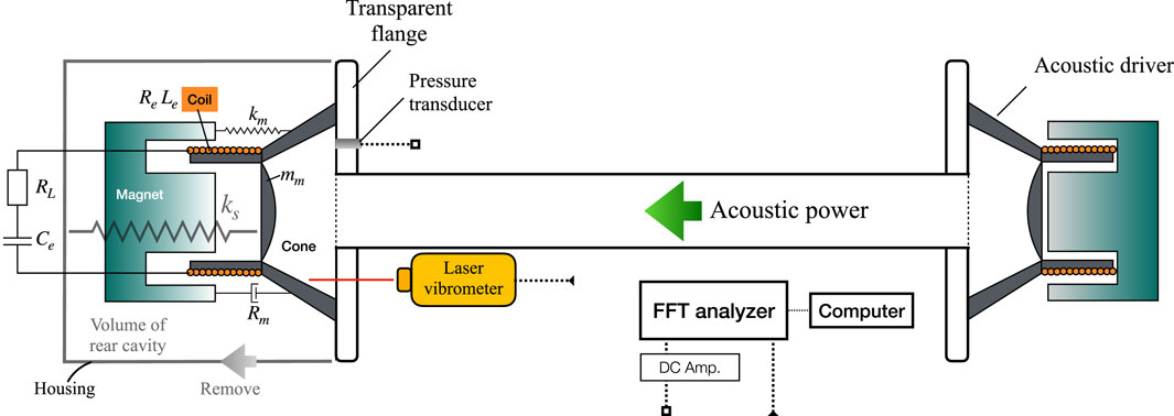
FIGURE 1. Experimental setup for examining the audio loudspeaker housing within the container.

By linear and harmonic approximations, a simple linear model (Kleiner, 2013; Swift, 2017) for an electrodynamic device in the frequency domain can be given as follows:

$\mathrm{\Delta }P=\frac{Bl}{A_m}I+\frac{Z_m}{A_m^2}{U}_{+}(\mathrm{1a})$

and

$U_{+}=\frac{A_m}{Bl}{Z}_{e}I.(\mathrm{1b})$

In Eqs 1a, 1b, U₊ stands for the complex amplitude of the volume velocity driven by the paper cone and A_m represents the effective surface area of the cone. Note that we suppose that the stiff paper cone is oscillated with a uniform velocity V₊. Therefore, the volume velocity U₊ driven by the cone is U₊ = V₊A_m. Bl denotes the force factor, and I represents the complex electric current through the coil. Note that Bl is the product of the magnetic-flux density B and the total effective length of the coil l. Furthermore, ΔP represents the complex amplitude of the oscillation pressure difference between pressure oscillation P₊ at the front and P_v at the rear of the cone, namely, ΔP = P₊−P_v. In the control equations of the loudspeaker, the mechanical impedance Z_m and the electrical impedance Z_e are, respectively, given as

$Z_m=R_m+i\left(\omega m_m-\frac{k_m}{\omega }\right)=R_m+i{X}_m(\mathrm{2a})$

and

$Z_e=R_e+R_L+i\left(\omega L_e-\frac{1}{\omega C_e}\right)=R_e+R_L+i{X}_e,(\mathrm{2b})$

where R_m, m_m, and k_m, respectively, denote the mechanical resistance, mass, and stiffness and X_m represents the mechanical reactance; R_e and L_e, respectively, symbolize the electrical resistance and inductance of the coil; and X_e stands for the electrical reactance. In addition, R_L and C_e, respectively, stand for the external electrical resistance and capacitance connected to the terminals of the coil as an electrical load for extracting electrical power.

Because the loudspeaker is set within the cavity volume of the container, the paper cone functions as a reciprocating piston on the gas column. The sealed volume of the rear cavity therefore functions as a gas spring k_s, which relates the back pressure oscillation P_v of the loudspeaker as $P_v=k_s{U}_{+}/i\omega$ (Swift, 2017; Beranek and Mellow, 2019; Garrett, 2020). The mechanical stiffness of the volume of gas, k_s, is theoretically given by the adiabatic gas assumption with

$k_s=\frac{\gamma P_m{A}_m^2}{V_v},(3)$

where γ is the ratio of the specific heats at constant pressure and constant volume, V_v is the volume of the rear cavity, and P_m is the mean pressure.

We replace P_v in terms of k_s in Eq. 1a and arrange Z_m in Eq. 2a by adding k_s in the stiffness term k_m in parallel, which gives total stiffness k_d of the loudspeaker system as k_d = k_m + k_s, which can be written as $X_m=\omega m_m-\left(k_d/\omega \right)$. Eliminating I in Eqs 1a, 1b yields the acoustic impedance of the audio loudspeaker as

$Z_a=\frac{P_{+}}{U_{+}}=\frac{1}{A_m^2}\left[\frac{{\left(Bl\right)}^2}{Z_e}+Z_m\right]\text{.}(4)$

We clearly express the real part and the imaginary part of Z_a with

$Z_a=\frac{1}{A_m^2}\left\{\left[R_m+\frac{\left(R_e+R_L\right){\left(Bl\right)}^2}{{\left(R_e+R_L\right)}^2+X_e^2}\right]+i\left[X_m-\frac{X_e{\left(Bl\right)}^2}{{\left(R_e+R_L\right)}^2+X_e^2}\right]\right\}\text{.}(5)$

As an acoustical load of the impedance shown in Eq. 5, the real part of Z_a mainly represents the dissipative term in acoustics, while the imaginary part of Z_a denotes the acoustic reactance. It is worth noting that the imaginary part of Z_a is mainly dominated by X_m due to the much smaller value of X_e. Since the acoustical load receives acoustic power generated from the engine, the sign of the acoustic impedance of the loudspeaker should align with the thermoacoustic engine in the calculation model. We use the equation

$Z_{sp}=-Z_a(6)$

to couple the loudspeaker model with the thermoacoustic theory.

2.2 Transfer matrices derived from Rott’s thermoacoustic theory

With Rott’s acoustic approximation (Tominaga, 1998; Swift, 2017) for small amplitude of gas oscillation with angular frequency ω, basic equations of energy, momentum, and continuity are linearized as the framework of thermoacoustic theory. For cylindrical pores with the gas-occupied cross-sectional area A, the thermoacoustic model in the frequency domain is expressed as follows:

$\left\{\begin{array}{c}\frac{dP}{dx}=-i\omega \frac{{\rho }_m}{A}\frac{1}{1-{\chi }_{\nu }}U=-\mathcal{Z}U\hfill \\ \frac{dU}{dx}=-i\omega \frac{A\left[1+\left(\gamma -1\right){\chi }_{\alpha }\right]}{\gamma P_m}P+\frac{{\chi }_{\alpha }-{\chi }_{\nu }}{\left(1-{\chi }_{\nu }\right)\left(1-\sigma \right)}\frac{1}{T_m}\frac{d{T}_m}{dx}U=-\mathcal{Y}P+\mathcal{G}U,\hfill \end{array}\right.(7)$

where P and U, respectively, stand for the complex amplitudes of the acoustic pressure and the complex amplitude of volumetric velocity. In the equations, $\mathcal{Z}$ stands for the fluid impedance per unit length, $\mathcal{Y}$ denotes the fluid admittance, and $\mathcal{G}$ represents the thermoacoustic source/damping term. Whether $\mathcal{G}$ is the source or damping term depends on the sign of the temperature gradient dT_m/dx. Note that the symbol σ in $\mathcal{G}$ represents the Prandtl number. Furthermore, χ_j (j = α or ν) is a thermoacoustic function, and subscripts ν and α, respectively, denote the viscous and the thermal effects (Swift, 2017; Biwa, 2021). If the geometries of flow channels are simple, χ_j is possible to be theoretically obtained (Swift, 2017; Biwa, 2021). It is worth noting that r/δ_j is a key non-dimensional parameter that dominates thermoacoustic functions, where δ_j $(=\sqrt{2j/\omega })$ represents the thermal or viscous penetration depths, using j = α or ν, respectively, for the thermal diffusivity or the kinematic viscosity of the working gas. For cylindrical tubes represented by radius r and parallel plates characterized by the half of spacing r_d, χ_j are calculated as

${\chi }_j=\left\{\begin{array}{cc}\frac{2J_1\left[\left(i-1\right)\frac{r}{{\delta }_j}\right]}{\left(i-1\right)\frac{r}{{\delta }_j}{J}_0\left[\left(i-1\right)\frac{r}{{\delta }_j}\right]}\hfill & \text{\hspace{0.17em}for\hspace{0.17em}circular\hspace{0.17em}pores}\hfill \\ \frac{\tanh \left[\left(1+i\right)\frac{r_{\text{d}}}{{\delta }_j}\right]}{\left(1+i\right)\frac{r_{\mathrm{d}}}{{\delta }_j}}\hfill & \text{for\hspace{0.17em}parallel\hspace{0.17em}plates}\hfill \end{array}\right.\text{,}(8)$

where δ_j $(=\sqrt{2j/\omega })$ represents the thermal or viscous penetration depths, using j = α or ν, respectively, for the thermal diffusivity or the kinematic viscosity of the working gas. Furthermore, J₀ is the zeroth order Bessel function of the first kind, and J₁ is the first-order Bessel function of the first kind. Drawing from the segments illustrated in Figure 2 and utilizing Eq. 8, we model the resonator tubes 1 and 2, branch resonator, thermal buffer tube, and stacked-screen regenerator using the circular cylindrical tube model, while the two heat exchangers are depicted through the theoretical expression for parallel plates. Importantly, even though the stacked-screen regenerator exhibits tortuous flow channels, we characterize it using cylindrical modeling with an effective radius, as reported by Ueda et al. (2009), when non-linear effects are negligible.

FIGURE 2

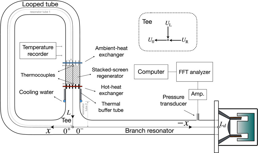
FIGURE 2. Experimental setup of the thermoacoustic Stirling engine loaded with the loudspeaker.

If the characteristic length or radius of cylindrical flow channels with simple and regular geometries are known, coefficients of $\mathcal{Z}$, $\mathcal{Y}$, and $\mathcal{G}$ can be considered constants for a short segment of length Δx. Combining Eq. 7 by eliminating U yields the Helmholtz equation for thermoacoustics, which is expressed as

$\frac{d^{2}P}{d{x}^2}-\mathcal{G}\frac{dP}{dx}-\mathcal{Y}\mathcal{Z}P=0.(9)$

By solving the aforementioned Helmholtz equation, we can obtain an acoustic network model for the whole system. With a transfer matrix M solved from Eq. 9, we therefore relate acoustic pressure P and volume velocity U at two ends of a short segment of length Δx as

$\left[\begin{array}{c}\hfill P\left(x+\mathrm{\Delta }x\right)\hfill \\ \hfill U\left(x+\mathrm{\Delta }x\right)\hfill \end{array}\right]=e^{\left(\frac{\mathcal{G}\mathrm{\Delta }x}{2}\right)}\left(\begin{array}{cc}\hfill -\frac{\mathcal{G}}{D}\sinh \left(\lambda \right)+\cosh \left(\lambda \right)\hfill & \hfill \frac{2\mathcal{Z}}{D}\sinh \left(\lambda \right)\hfill \\ \hfill \frac{2\mathcal{Y}}{D}\sinh \left(\lambda \right)\hfill & \hfill \frac{\mathcal{G}}{D}\sinh \left(\lambda \right)+\cosh \left(\lambda \right)\hfill \end{array}\right)\left[\begin{array}{c}\hfill P\left(x\right)\hfill \\ \hfill U\left(x\right)\hfill \end{array}\right],(10)$

with $D=\sqrt{{\mathcal{G}}^2+4\mathcal{Y}\mathcal{Z}}$ and λ = DΔx/2. Characterizing every element of the acoustic duct using Eq. 10 enables us to theoretically describe a matrix M_loop = M_tube,2M_TBTM_HM_REGM_RM_tube,1 for the looped part of the thermoacoustic engine, where subscript tube, 1 or 2, R, REG, H, and TBT of matrices M denote the 30-mm-diameter waveguide tube, ambient-heat exchanger, stacked-screen regenerator, hot-heat exchanger, and thermal buffer tube, respectively. Note that we divide M_REG and M_TBT into 100 parts to describe axially linear temperature distributions imposed on these two regions, for accounting for the thermal properties of the working gas. By considering continuity at the T-junction, acoustic states at the origin are realized with U₀ = U_L + U_R (referring to the inset of Figure 2) and P₀ = P_L, where subscripts 0, L, and R, respectively, indicate acoustic states at positions of x = 0⁺ m, x = 1.635 m, and x = 0⁻ m, as illustrated in Figure 2. As a result, the transfer matrix M_loop can relate acoustic states at two ends of the looped part of the engine, through the continuity of P(x = 0) = P(x = L) and U(x = 0⁺) = U(x = 0⁻) + U(x = L), with

$\left[\begin{array}{c}\hfill P_{\text{L}}\hfill \\ \hfill U_{\text{L}}\hfill \end{array}\right]=M_{\text{loop}}\left[\begin{array}{c}\hfill P_0\hfill \\ \hfill U_{\text{R}}+U_{\text{L}}\hfill \end{array}\right]\text{.}(11)$

Furthermore, acoustic states at two ends of the branch resonator are related by M_BR using Eq. 10 without any temperature gradients as

$M_{\text{BR}}\left[\begin{array}{c}\hfill P_{\text{en}}\hfill \\ \hfill U_{\text{en}}\hfill \end{array}\right]=\left[\begin{array}{c}\hfill P_0\hfill \\ \hfill U_{\text{R}}\hfill \end{array}\right]\text{,}(12)$

where the subscript en represents the acoustic state at x = L_d = 1.494 m, which is the sum of the length of the branch resonator and the thickness of the front plate of the loudspeaker housing. We obtain the acoustic impedance Z_en at L_d by relating Eq. 11 and Eq. 12 with the continuity at the T-junction of x = 0, which is expressed as follows:

$Z_{\text{en}}=\frac{P_{\text{en}}}{U_{\text{en}}}.(13)$

The acoustic impedance of the loudspeaker, Z_sp, represented by Eq. 6, should serve as the boundary conditions at the interface between the thermoacoustic engine and the loudspeaker. Replacing Z_sp of Eq. 6 with Z_en in Eq. 12 results in

$\begin{array}{cccc}\hfill \left[\begin{array}{c}\hfill P_0\hfill \\ \hfill U_{\text{R\hspace{0.17em}}}\hfill \end{array}\right]\hfill & =M_{\text{BR}}\hfill & \hfill \left[\begin{array}{c}\hfill Z_{sp}\hfill \\ \hfill 1\hfill \end{array}\right]\hfill & \hfill \left(-U_{+}\right)\hfill \\ \hfill \hfill & =\left(\begin{array}{cc}\hfill m_{11}\hfill & \hfill m_{12}\hfill \\ \hfill m_{21}\hfill & \hfill m_{22}\hfill \end{array}\right)\hfill & \hfill \left[\begin{array}{c}\hfill Z_{sp}\hfill \\ \hfill 1\hfill \end{array}\right]\hfill & \hfill \left(-U_{+}\right),\hfill \end{array}(14)$

where m denotes elements of the matrix M_BR. Eliminating U₊ in Eq. 14 gives the relationship between U_R and P₀ as

$U_{\text{R}}=\frac{m_{21}{Z}_{sp}+m_{22}}{m_{11}{Z}_{sp}+m_{12}}{P}_0.(15)$

Equation 15 enables us to rewrite Eq. 11 as

$\begin{array}{ccc}\hfill \left[\begin{array}{c}\hfill P_{\text{L}}\hfill \\ \hfill U_{\text{L\hspace{0.17em}}}\hfill \end{array}\right]\hfill & \hfill =M_{\text{loop}}\left(\begin{array}{cc}\hfill 1\hfill & \hfill 0\hfill \\ \hfill \frac{m_{21}{Z}_{sp}+m_{22}}{m_{11}{Z}_{sp}+m_{12}}\hfill & \hfill 1\hfill \end{array}\right)\hfill & \hfill \left[\begin{array}{c}\hfill P_{\text{L}}\hfill \\ \hfill U_{\text{L}}\hfill \end{array}\right],\hfill \\ \hfill \hfill & =M_{\text{All}}\hfill & \hfill \left[\begin{array}{c}\hfill P_{\text{L}}\hfill \\ \hfill U_{\text{L}}\hfill \end{array}\right]\hfill \end{array}(16)$

where M_All stands for a representative transfer matrix of the combined system. Nonzero ${[P_{\text{L}},A{U}_{\text{L}}]}^{⊺}$ in Eq. 16 results in a characteristic equation as

$\det \left[M_{\text{All}}-E\right]=0\text{,}(17)$

where E represents the identity matrix and det[ ] stands for the determinant of a matrix.

In this study, we used the numerical solver “fsolve” in MATLAB (MathWorks, Inc.) and set the tolerance at TolFun = 10^–25 to solve the aforementioned characteristic equation. Although the acoustical load of the loudspeaker strongly influences the fundamental frequency of the combined system, an initial guessing angular frequency ω₀ = 2πa/(L + L_d) × 1/4 = 174.6 rad/s, equivalent to 27.8 Hz, approximately estimated from the engine part is adopted for numerically solving Eq. 17, where a represents the adiabatic speed of sound for the working gas at the room temperature of 298 K. If a temperature difference across the regenerator is assigned, solving Eq. 17 yields a complex value of the angular frequency ω = ω_R + iω_I (Hsu and Li, 2023), where ω_R stands for the angular frequency of acoustic oscillation and ω_I represents the growth rate (ω_I < 0) or attenuation rate (ω_I > 0) over time, depending on the imposed temperature difference. In the light of |ω_I| < 10^–8, solutions of Eq. 17 provide the onset temperature difference and the frequency of the spontaneous oscillation for the thermoacoustic engine loaded with the loudspeaker.

3 Experiments

3.1 Experimental determination of acoustic characteristics of the audio loudspeaker unit

A commercially available audio loudspeaker (Fostex FW168HS, Foster, Tokyo, Japan), having high stiffness diaphragm of the paper cone, is mounted in the circular center of a 15-mm-thick transparent flange of the container that is part of a stainless steel cylinder container with an inner diameter of 30 cm and an inner axial length of 34 cm. Table 1 lists detailed specifications and measured Thiele/Small (T/S) parameters of the commercial loudspeaker Fostex FW168HS used in the present study. The T/S parameters of the audio loudspeaker mounted in the container were measured according to the instructions provided in the acoustic textbook (Yu et al., 2011; Garrett, 2020). The moving mass m_m and stiffness k_m were measured by plotting the relationships between adding known masses on m_m and resonance frequencies of the loudspeaker. For the gas spring effect resulting from the volume of the rear cavity, we tested the audio speaker within and without the housing for experimentally determining the stiffness k_s, by monitoring the changes in resonance frequencies. The mechanical resistance R_m was determined using a simple free-decay experiment, while the internal electrical resistance R_e and inductance L_e of the coil were simply probed using a volt-ohm-milliammeter. Furthermore, the coil of the audio loudspeaker connects with resistances R_L and capacitance C_e in series as experimental variables for modulating the acoustic impedance. The influence both on the real and imaginary parts can be realized in Eq. 5.

TABLE 1

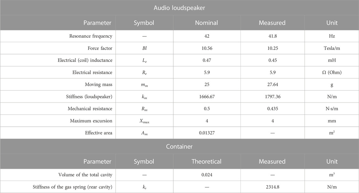
TABLE 1. Specifications of the audio loudspeaker Fostex FW168HS.

In addition to examining the T/S parameters of the audio loudspeaker individually, we measured ΔP and U₊ to experimentally determine Z_sp, supposing the uniform oscillation velocity V₊ across the paper cone. Figure 1 illustrates the experimental setup used to ascertain the acoustic impedance of the loudspeaker. Another loudspeaker, acting as an acoustic driver, was attached at the end of a duct and positioned opposite the test loudspeaker. A pressure transducer (PMS-5M-2-1M, JTEKT, Nagoya, Japan) was mounted at the transparent front flange of the loudspeaker to measure P₊. It is important to note that we determine P₊ as ΔP since the loudspeaker was tested with the housing removed to simplify concerns related to the effects of the rear cavity. Through the pressure transducer, signals of the pressure oscillations were amplified 2,000 times by DC Amplifiers (AA6210, JTEKT, Nagoya, Japan) and then recorded using a fast Fourier transform (FFT) analyzer (OR35, OROS, Grenoble, French). To determine the oscillating velocity V₊ of the paper cone, a laser vibrometer (PDV-100, Polytec, Waldbronn, Germany) was utilized. This device measured the oscillation velocity of the cone by passing a laser beam through the transparent flange to probe the paper cone. The signals generated by the vibrometer were recorded using the FFT analyzer along with the pressure signals. By reading peak values from the amplitude spectrum and phase spectrum via the fast Fourier transform algorithm, measured acoustic states were presented with the acoustic pressure $p(x)=\mathrm{R}\mathrm{e}\left[P(x)e^{i\omega t}\right]$ and the oscillation volume velocity $u(x)=\mathrm{R}\mathrm{e}\left[U(x)e^{i\omega t}\right]$. We generated acoustic waves by driving the loudspeaker using a power amplifier (PX3, Yamaha, Shizuoka, Japan) and a function generator. Since we aimed to match the load impedance with the engine part at the initial onset states, a low amplitude of acoustic forcing was conducted for the experiments.

3.2 Experimental setup of the combined system

A schematic model has been illustrated in Figure 2 for our prototype of the thermoacoustic electric generator examined in this study. The prototype consists of the engine part and the load part, which were filled with ambient air at atmospheric pressure. The acoustic load part is the loudspeaker in the container mentioned in Section 3.1. The cone of the loudspeaker is set toward the engine part for receiving the acoustic power delivered from the engine part. The engine part is constructed using a 30-mm-inner-diameter tube of stainless steel, which can be divided by an averaged 1.635-m-long looped tube and a branch resonator tube of 1.479 m long. A pressure transducer (PMS-5M-2-1M) is mounted at x = −1.279 m to monitor pressure fluctuations of the gas column. The looped tube contains the thermoacoustic core consisting of a regenerator sandwiched between the hot- and ambient-heat exchangers. A thermal buffer tube is attached at one end of the hot-heat exchanger to moderate the thermal impact on the looped tubes. The heat exchangers consist of numerous brass fins with 0.5 mm in thickness and 1 mm spacing, which are inserted with three brass tubes, respectively, for installing electrical cartridge heaters and circulating cooling water. The geometrical parameters of the thermoacoustic system are shown in Table 2. Furthermore, the regenerator is made of a pile of stainless 304 wire woven mesh screens of #60 whose hydraulic diameter d_h and wire diameter d_w are, respectively, 0.4031 and 0.15 mm. The effective radius of empirical expressions (Ueda et al., 2009) for the stacked-screen regenerator, $r_0=\sqrt{d_{\text{h}}{d}_{\text{w}}}/2$, is used to model its flow channels for modeling into the linear theoretical framework. Two type-K thermocouples are inserted at both ends of the regenerator to observe the axial temperature difference ΔT = T_H−T_C across the regenerator, where T_H and T_C, respectively, represent the temperatures at the hot and ambient sides of the regenerator. To monitor these temperatures and record their time series data, we utilized a temperature recorder (LR8450, Hioki, Ueno, Japan) with a sampling interval set at 1 s.

TABLE 2

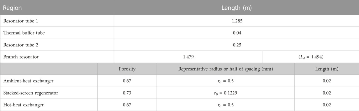
TABLE 2. Geometric parameters of the thermoacoustic engine.

3.3 Error analysis

In this study, we measured pressure, frequency, temperature, and velocity. We used a PMS-5M-2 pressure transducer to conduct pressure measurements, with a sensitivity of 7.49 Pa/mV and an accuracy within 0.15% FS for readings smaller than 2 kPa. The voltage-represented pressure signal is amplified 2,000 times using the DC amplifier (AA6210), which would introduce a peak-to-peak voltage noise of 15 μV, resulting in a maximum noise error of less than 0.1 Pa. The amplified voltage signals are subsequently analyzed using the OROS OR35 spectrum analyzer, which operates with 25,601 sampling points at a sampling frequency of 3276.8 Hz. The relative precision of frequency is within 1⁻⁵. It is worth noting that the sampling frequency is substantially higher than the maximum frequency (below 40 Hz) examined in this study. The OROS OR35 has a resolution of 24 bits with a dynamic range of 144 dB. When it is used to process voltage signals from the DC amplifier in the range of ±1 V, it is capable of discerning signal changes down to 0.1 μV. Temperatures are measured with type-K thermocouples (T35165H), which have an accuracy of ±2.5 K over the range of 273–923 K. We recorded the probed temperatures using the Hioki LR8450 temperature recorder, which maintains an accuracy of ±0.5 K within the range of 273–773 K and a resolution of 1 μV when used in the range of ±20 mV, corresponding to the type-K thermocouple. Furthermore, velocity is determined using the PDV-100 laser vibrometer, which has an accuracy of 1% FS within a range of ±100 mm/s.

The systematic measurement error σ_sys and random error σ_ran are, respectively, given as

${\sigma }_{\text{mea}}=\sqrt{{\sigma }_{\text{sys}}^2+{\sigma }_{\text{ran}}^2}(18)$

and

${\sigma }_{\mathrm{r}\mathrm{a}\mathrm{n}}=\frac{\sqrt{\frac{\sum _{j=1}^n{\left(y_j-\overline{y_j}\right)}^2}{n-1}}}{\sqrt{n}},(19)$

where y_j represents the jth measurement, $\overline{y_j}$ is the arithmetic mean of measurements, and n is the number of repeated measurements. The systematic error σ_sys is due to the accuracy of the measurement devices, and the random error σ_ran is the standard deviation of repeated experiments. Note that not every physical quantity was subjected to repeated measurements in the present study. For these instances, we calculate the random error using ${\sigma }_{\text{ran}}=\frac{1}{2}(\text{resolution\hspace{0.17em}of\hspace{0.17em}device})/\sqrt{3}$, where the term $\sqrt{3}$ originates from the assumption of a rectangular distribution of the measurement values’ probabilities¹.

Through these calculations, we estimated the maximum measurement errors for pressure, frequency, temperature, and velocity to be ±3.00 Pa, ±0.003 Hz, ±3.00 K, and ±1.00 mm/s, respectively.

3.4 Measuring onset thresholds of the combined system

For starting the thermoacoustic engine loaded with the loudspeaker, we introduce the external heat power through the power supply to electrical cartridge heaters at the hot-heat exchanger and circulate the cooling water through the ambient-heat exchanger to maintain a constant temperature of T_C = 298 K, to impose steep temperature gradients on the regenerator axially. In the experiments, we ensured thermally steady states to maintain a stable temperature difference ΔT. This stable ΔT was critical for reaching the instability threshold. Once this threshold was crossed, it triggered spontaneous pressure oscillations in the gas column, consistently coupled with the loudspeaker. The thermoacoustic engine loaded with the loudspeaker was thus excited in the natural resonant frequency of the combined system.

Figure 3 illustrates an example of our experimental approach, showcasing time-series data of both acoustic pressure and temperatures during the transition from a stable state to spontaneous oscillation states. During the startup phase, spontaneous oscillations within the gas column emerge at approximately 700 s, coinciding with a gradual increment of T_H at 0.85 K/min. In the spontaneous oscillation states, temperatures remain generally stable within specific ranges, specifically T_H within 3 K and T_C within 0.5 K. These stable conditions allowed us to experimentally determine the onset temperature difference based on these steady temperatures, thus demonstrating the practical application and validity of our experimental setup.

FIGURE 3

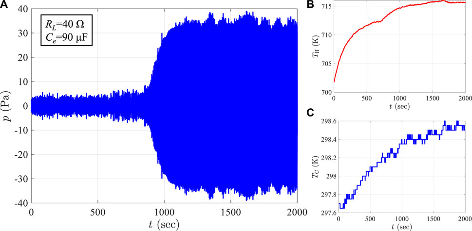
FIGURE 3. Measured time-series acoustic pressure (A) at x = −1.279 m and temperatures of the hot (B) and ambient (C) ends of the regenerator.

4 Results and discussion

4.1 Calibrations of the audio loudspeaker

The measurements of Z_sp, obtained from forced oscillation experiments on the acoustic driver at low amplitudes of acoustic forcing (below 100 Pa, monitored by P₊), are shown in Figure 4. Given the low amplitude of acoustic forcing, we assume that the input impedance of the loudspeaker remains unaffected by the amplitude of oscillation pressure. We conducted tests on the loudspeaker using forced steady oscillations at frequencies of 10, 20, 30, and 40 Hz. These test points are represented by black dots in the figure, while the real and the imaginary parts of Z_sp are shown on the separate vertical axes in two subfigures (a) and (b) in Figure 4. Note that every data point we plotted represents the mean of six repeated measurements. We used Eq. 19 to determine the random error, which is represented as the standard deviation shown in the attached error bars. Detailed information about the means of the measurements and corresponding standard deviations can be found in Table 3. The red curve illustrates the theoretical estimation from the linear model presented in Eq. 6. The T/S parameters used by the linear model depicted in Section 3.1 are each measured and detailed in Table 1.

FIGURE 4

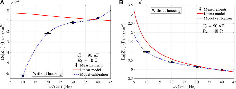
FIGURE 4. Comparisons of Z_sp among measurements, linear model, and calibration. (A) represents the real part of Z_sp and (B) represents the imaginary part.

TABLE 3

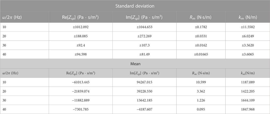
TABLE 3. Means and standard deviations (σ_ra, with n = 6) of measurements shown in Figure 4 and Figure 5.

Despite removing the loudspeaker housing to minimize the effects of the complex geometry in the loudspeaker’s rear cavity, the real part of the measured Z_sp deviated significantly from the theoretical prediction of the linear model. This deviation could be attributed to the geometry of the front cavity formed by the paper cone, highlighting the difficulties in accurately measuring mechanical resistance through the simple free amplitude decay experiments. However, the imaginary components of Z_sp exhibited qualitative consistency with the theoretical estimations. To mitigate these discrepancies, we calibrated the linear model based on the measurements of Z_sp.

Considering the linear model of the loudspeaker, as shown in Eq. 5, the real part of Z_a is primarily determined by the sum of the electrical resistances R_e + R_L and mechanical resistance R_m, while the imaginary part of Z_sp is influenced by the mechanical stiffness k_m of the loudspeaker since X_m ≫ X_e. Assuming constant values for electrical components, we can determine R_m and k_m from the measured Z_sp using the linear model shown in Eq. 5 while keeping the other T/S parameters constant. This calibration is achieved through the following equations:

$R_m=-A_m^2\mathrm{R}\mathrm{e}\left[Z_{sp}\right]-\mathrm{R}\mathrm{e}\left[\frac{{\left(bl\right)}^2}{Z_e}\right],(20)$

$k_m=\omega A_m^2\mathrm{I}\mathrm{m}\left[Z_{sp}\right]+{\omega }^2{m}_m.(21)$

The calibration values of R_m and k_m are, respectively, displayed in the subfigures (a) and (b) of Figure 5. As observed, R_m exhibits a cubic polynomial function of the frequency, while k_m demonstrates a nearly linear relationship with the frequency. Consequently, regression fitting is employed to obtain the following regression functions:

$\left\{\begin{array}{cc}\hfill R_m& =-0.000682{\left(\frac{\omega }{2\pi }\right)}^3+0.0665{\left(\frac{\omega }{2\pi }\right)}^2+-2.2398\left(\frac{\omega }{2\pi }\right)+27.033,\hfill \\ \hfill k_m& =22.0454\left(\frac{\omega }{2\pi }\right)+974.208\hfill \end{array}\right.(22)$

FIGURE 5

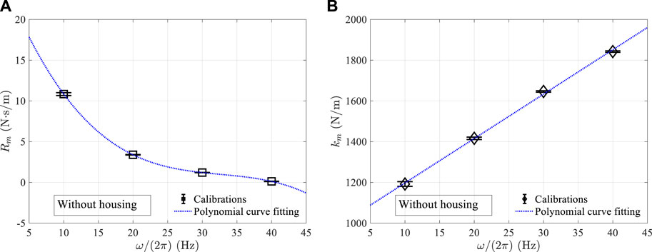
FIGURE 5. Calibrated results: (A) mechanical resistance R_m and (B) mechanical stiffness k_m, where markers are the calibration values obtained from Eqs 20, 21, and dotted curves are regressed polynomial functions according to the calibration values.

By incorporating the regression functions of R_m and k_m into Eq. 6, we obtained the calibrated Z_sp represented by the blue dotted curves in Figure 4. As evident from the figure, the calibrated Z_sp accurately reproduces the measured data. With Eq. 6 calibrated using R_m and k_m, we can effectively model the loudspeaker for practical scenarios within the tested frequency range of 10–40 Hz while considering the absence of significant amplitude effects.

4.2 Onset conditions of the combined system

Figure 6 illustrates the onset conditions of the thermoacoustic Stirling engine when loaded with the audio loudspeaker. The figure consists of the following two subfigures: (a) representing the onset temperature difference T_H−T_C and (b) representing the spontaneous oscillation frequency ω/(2π). Both subfigures are plotted on a logarithmic horizontal axis, with the external electrical resistance R_L parameterized accordingly. In Figure 6, experiments of the thermoacoustic engine loaded with the loudspeaker are denoted by markers (◦ for housing and * for no housing), while the theoretical estimation, obtained by solving the characteristic Eq. 17 using the calibrated loudspeaker model, is represented by curves (solid for housing and dotted for no housing). The spontaneous steady oscillation states are confirmed over a range of 20 Ω < R_L < 1,000 Ω. Note that for the analytical estimations involving the loudspeaker with housing, the calibrated values of R_m and k_m used in the model are obtained from the case without housing. To incorporate the housing effect, we include the measured gas spring k_s to account for the total mechanical stiffness k_d.

FIGURE 6

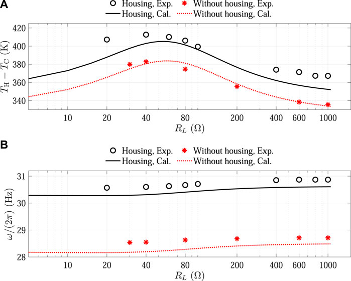
FIGURE 6. Onset conditions of the thermoacoustic Stirling engine loaded with the loudspeaker, tested under C_e = 90 μF while varying R_L: (A) onset temperature difference and (B) spontaneous oscillation frequency.

When examining the onset temperature difference ΔT of the combined system illustrated in Figure 6A, it can be observed that both the loaded loudspeaker with and without housing exhibit a hill-like trend as a function of the logarithmic horizontal axis R_L, which affects the onset temperature difference by approximately 20 K. The observation in Figure 6A suggests that ΔT reaches maximum values when R_L is approximately in the range of 40–80 Ω. Figure 6B demonstrates that the spontaneous oscillation frequency slightly increases with R_L by approximately 0.4 Hz, and this can be qualitatively explained by the expression of Im (Z_a) in Eq. 5. It is realized that the acoustic reactance is minimally affected by R_L due to the dominance of X_e over X_m.

From Figure 6, it can be noted that the experimental measurements align reasonably well with the calculated results. By analyzing the onset temperature difference of the combined system, as depicted in Figure 6A, it becomes evident that the case of the audio loudspeaker without housing exhibits better consistency than that with housing. In Figure 6B, precise estimations for the onset frequency are displayed, with discrepancies of less than 0.5 Hz observed for both cases of the loudspeaker with and without housing. Notably, the case of the loudspeaker without housing demonstrates good agreement, with a maximum deviation of 1.7% observed at the data point of 80 Ω.

It is worth noting that in our previous research (Hsu and Li, 2023), we found a satisfactory level of consistency in the #60 stacked-screen regenerator, with discrepancies of approximately 18%. This was observed when using resonators with slightly varying lengths in the current thermoacoustic Stirling engine in the absence of any acoustical load. However, in the current study, we used the same regenerator in the loaded engine and found improved agreements, particularly when the loudspeaker was loaded on the engine in the case without housing. In this loaded thermoacoustic engine scenario, it is likely that the system experiences larger dissipation mechanisms. This infers that the sensitivity of the onset temperature estimation is intrinsically limited to a well-accepted fact, namely, that the onset ΔT is achieved when the thermoacoustic power generation slightly surpasses the dissipation at minimal oscillation amplitudes. Hence, once the load model is precisely theoretically estimated, implementing an appropriate acoustic load could help mitigate this sensitivity.

On the other hand, the larger discrepancies observed in the case of the loaded loudspeaker with housing could be attributed to the dissipation term in the rear cavity not being incorporated into the calculation model. In the calibration procedure for R_m and k_m for this study, we have only considered the front cavity of the paper cone. Furthermore, we simply account for the gas spring effect of the rear cavity in the loudspeaker housing. However, the complex geometries formed in the front and rear of the paper cone of the loudspeaker likely introduce non-negligible minor losses. This could be the primary reason for the larger discrepancies observed in our comparisons between calculations and experiments.

It should be noted that, in the range of 40–80 Ω, the comparisons agree relatively well. The higher onset temperature differences in the range of 40–80 Ω indicate that the system needs to overcome a greater load resistance, which our model predicts reasonably. However, for relatively lower onset temperature differences, the influence of the loudspeaker housing may affect accuracy, highlighting areas where our model’s predictive capability could be further improved.

Zorgnotti et al. (2018) highlighted this issue and carried out calibrations to experimentally determine the acoustic admittances of the two cavities by measuring the acoustic impedance through a two-load method. Their work not only is applicable to the engine onset but also has the capability of estimating larger limit cycle amplitudes of a loaded thermoacoustic engine through impedance matching. Our current research, which is based on solving the characteristic equation of the combined system, could benefit from the adoption of their calibration techniques.

In contrast, C_e directly impacts the imaginary part of Z_a. While maintaining R_L = 40 Ω, we also varied C_e to experimentally observe the applicability of the current calibration in describing the onset conditions of the combined system, as shown in Figure 7. The representations of markers and curves in Figure 7 are the same as in Figure 6, except for the horizontal axis which denotes C_e as the experimental parameter, ranging from 40 to 1,000 μF. In Figure 7A, it can be observed that measurements of the loaded loudspeaker, whether with or without housing, demonstrate a gradual increase with respect to the logarithmic C_e axis, indicating an approximate increase of 100 K in ΔT. The consistency between measurements and calculations for onset ΔT is only valid in the range from 40 to 200 μF. Because our calibration for k_m assumes X_m ≪ X_e, larger C_e values would introduce significant effects for X_e, leading to discrepancies. Meanwhile, as illustrated in Figure 7B, the current calculation model, based on the present loudspeaker calibration, well predicts spontaneous oscillation frequencies as C_e varies.

FIGURE 7

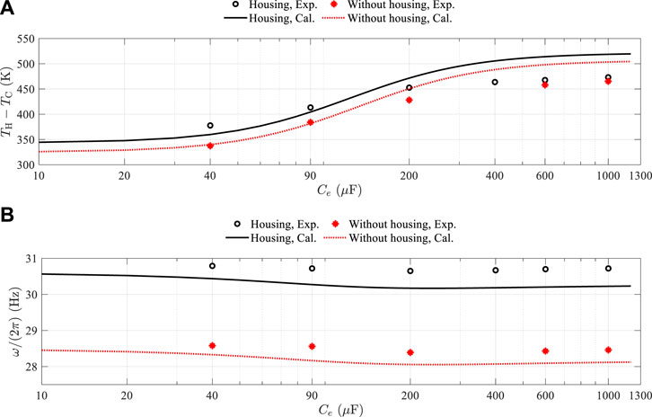
FIGURE 7. Onset conditions of the thermoacoustic Stirling engine loaded with the loudspeaker, tested under R_L = 40 Ω while varying C_e: (A) onset temperature difference and (B) spontaneous oscillation frequency.

5 Conclusion

This study estimates the onset conditions of a thermoacoustic Stirling engine loaded with an audio loudspeaker. This was achieved through comparisons of theoretical calculations, derived from the framework of the thermoacoustic theory combined with a linear loudspeaker model, and experimental observations, subsequently calibrated to accurately reflect measured data. The calibration of the loudspeaker model relied on the measurements of the loudspeaker’s impedance Z_sp, revealing noteworthy differences between theoretical predictions and experimental observations. These differences were considerably minimized by calibrating the mechanical resistance R_m and mechanical stiffness k_m, leading to a well-represented model of the loudspeaker within the tested frequency range of 10–40 Hz, under the small oscillation pressure amplitudes of less than 100 Pa. We subsequently examined the onset behaviors of the combined system comprising the thermoacoustic engine and the loudspeaker. The onset temperature differences across the regenerator and spontaneous oscillation frequencies were measured for comparison with the theoretical estimations using the calibrated loudspeaker model. In both scenarios of the loaded loudspeaker with and without housing, we observed a reasonable agreement between the calculated results and measurements. The case of the loudspeaker without housing showed a better agreement. Our observations highlighted the effects of the loudspeaker housing in which the dissipation term in the rear cavity of the speaker was not adequately represented in our calculation model. The complex geometry formed by the paper cone of the loudspeaker introduced minor but non-negligible losses, primarily responsible for the larger observed discrepancies between calculations and experiments. Future research efforts would benefit from adopting calibration techniques to experimentally determine the acoustic properties of the cavities of the loudspeaker housing in a container. In conclusion, our study offers valuable insights into the estimation of the onset conditions of a thermoacoustic Stirling engine equipped with an audio loudspeaker. It demonstrates the ability of analytical descriptions within Rott’s theoretical framework coupled with an acoustic load model. Moreover, for modeling a thermoacoustic engine equipped with a cost-effective alternator such as a commercially available loudspeaker, this study highlights the necessity for accurate calibration and considerations of complex geometries in the acoustic load for precise theoretical estimations.

Data availability statement

The original contributions presented in the study are included in the article/Supplementary material; further inquiries can be directed to the corresponding author.

Author contributions

S-HH: conceptualization, supervision, funding acquisition, resources, methodology, software, writing–original manuscript, and writing–review and editing. C-HL: investigation, experiments, and software. All authors contributed to the article and approved the submitted version.

Funding

This research was funded by the Project for the Junior Researcher of the National Science and Technology Council, Taiwan, under Grant Number NSTC 112-2221-E-027-105.

Conflict of interest

The authors declare that the research was conducted in the absence of any commercial or financial relationships that could be construed as a potential conflict of interest.

Publisher’s note

All claims expressed in this article are solely those of the authors and do not necessarily represent those of their affiliated organizations, or those of the publisher, the editors, and the reviewers. Any product that may be evaluated in this article, or claim that may be made by its manufacturer, is not guaranteed or endorsed by the publisher.

Footnotes

¹Based on “Measurement Uncertainty” guidelines provided by National Instruments.

References

Abdoulla-Latiwish, K. O., and Jaworski, A. J. (2019). Two-stage travelling-wave thermoacoustic electricity generator for rural areas of developing countries. Appl. Acoust. 151, 87–98. doi:10.1016/j.apacoust.2019.03.010

CrossRef Full Text | Google Scholar

Abdoulla-Latiwish, K. O., Mao, X., and Jaworski, A. J. (2017). Thermoacoustic micro-electricity generator for rural dwellings in developing countries driven by waste heat from cooking activities. Energy 134, 1107–1120. doi:10.1016/j.energy.2017.05.029

CrossRef Full Text | Google Scholar

Backhaus, S., and Swift, G. (1999). A thermoacoustic stirling heat engine. Nature 399, 335–338. doi:10.1038/20624

CrossRef Full Text | Google Scholar

Beranek, L., and Mellow, T. (2019). Acoustics: sound fields, transducers and vibration. second edn. United States: Academic Press. doi:10.1016/C2017-0-01630-0

CrossRef Full Text | Google Scholar

Bi, T., Wu, Z., Zhang, L., Yu, G., Luo, E., and Dai, W. (2017). Development of a 5 kw traveling-wave thermoacoustic electric generator. Appl. energy 185, 1355–1361. doi:10.1016/j.apenergy.2015.12.034

CrossRef Full Text | Google Scholar

Biwa, T. (2021). Introduction to thermoacoustic devices. Singapore: World Scientific. doi:10.1142/y0023

CrossRef Full Text | Google Scholar

Biwa, T., Watanabe, T., and Penelet, G. (2020). Flywheel-based traveling-wave thermoacoustic engine. Appl. Phys. Lett. 117, 243902. doi:10.1063/5.0022315

CrossRef Full Text | Google Scholar

Castrejón-Pita, A., and Huelsz, G. (2007). Heat-to-electricity thermoacoustic-magnetohydrodynamic conversion. Appl. Phys. Lett. 90, 174110. doi:10.1063/1.2733026

CrossRef Full Text | Google Scholar

Chen, G., Tang, L., and Yu, Z. (2020). Underlying physics of limit-cycle, beating and quasi-periodic oscillations in thermoacoustic devices. J. Phys. D Appl. Phys. 53, 215502. doi:10.1088/1361-6463/ab7a57

CrossRef Full Text | Google Scholar

Garrett, S. L. (2020). Understanding acoustics: an experimentalist’s view of sound and vibration. second edn. New York: Springer International Publishing. doi:10.1007/978-3-030-44787-8

CrossRef Full Text | Google Scholar

Gonen, E., and Grossman, G. (2014). Effect of variable mechanical resistance on electrodynamic alternator efficiency. Energy Convers. Manag. 88, 894–906. doi:10.1016/j.enconman.2014.09.024

CrossRef Full Text | Google Scholar

Hsu, S., and Li, Y. (2023). Estimation of limit cycle amplitude after onset threshold of thermoacoustic stirling engine. Exp. Therm. Fluid Sci. 147, 110956. doi:10.1016/j.expthermflusci.2023.110956

CrossRef Full Text | Google Scholar

Kang, H., Cheng, P., Yu, Z., and Zheng, H. (2015). A two-stage traveling-wave thermoacoustic electric generator with loudspeakers as alternators. Appl. Energy 137, 9–17. doi:10.1016/j.apenergy.2014.09.090

CrossRef Full Text | Google Scholar

Kleiner, M. (2013). Electroacoustics. United States: CRC Press. doi:10.1201/b13859

CrossRef Full Text | Google Scholar

Marx, D., Mao, X., and Jaworski, A. (2006). Acoustic coupling between the loudspeaker and the resonator in a standing-wave thermoacoustic device. Appl. Acoust. 67, 402–419. doi:10.1016/j.apacoust.2005.08.001

CrossRef Full Text | Google Scholar

Murti, P., Shoji, E., and Biwa, T. (2023). Analysis of multi-cylinder type liquid piston stirling cooler. Appl. Therm. Eng. 219, 119403. doi:10.1016/j.applthermaleng.2022.119403

CrossRef Full Text | Google Scholar

Penelet, G., Watanabe, T., and Biwa, T. (2021). Study of a thermoacoustic-stirling engine connected to a piston-crank-flywheel assembly. J. Acoust. Soc. Am. 149, 1674–1684. doi:10.1121/10.0003685

PubMed Abstract | CrossRef Full Text | Google Scholar

Piccolo, A. (2018). Design issues and performance analysis of a two-stage standing wave thermoacoustic electricity generator. Sustain. Energy Technol. Assessments 26, 17–27. doi:10.1016/j.seta.2016.10.011

CrossRef Full Text | Google Scholar

Saha, C., Riley, P. H., Paul, J., Yu, Z., Jaworski, A., and Johnson, C. (2012). Halbach array linear alternator for thermo-acoustic engine. Sensors Actuators A Phys. 178, 179–187. doi:10.1016/j.sna.2012.01.042

CrossRef Full Text | Google Scholar

Swift, G. W. (2017). Thermoacoustics: a unifying perspective for some engines and refrigerators. second edn. New York: Springer International Publishing. doi:10.1007/978-3-319-66933-5

CrossRef Full Text | Google Scholar

Timmer, M. A., de Blok, K., and van der Meer, T. H. (2018). Review on the conversion of thermoacoustic power into electricity. J. Acoust. Soc. Am. 143, 841–857. doi:10.1121/1.5023395

PubMed Abstract | CrossRef Full Text | Google Scholar

Timmer, M. A., and van der Meer, T. H. (2019). Characterization of bidirectional impulse turbines for thermoacoustic engines. J. Acoust. Soc. Am. 146, 3524–3535. doi:10.1121/1.5134450

PubMed Abstract | CrossRef Full Text | Google Scholar

Timmer, M. A., and van der Meer, T. H. (2020). Optimizing bidirectional impulse turbines for thermoacoustic engines. J. Acoust. Soc. Am. 147, 2348–2356. doi:10.1121/10.0001067

PubMed Abstract | CrossRef Full Text | Google Scholar

Tominaga, A. (1998). Fundamental thermoacoustics (in Japanese). Tokyo: Uchida Rokakuho Publishing Co.

Google Scholar

Ueda, Y., Kato, T., and Kato, C. (2009). Experimental evaluation of the acoustic properties of stacked-screen regenerators. J. Acoust. Soc. Am. 125, 780–786. doi:10.1121/1.3056552

PubMed Abstract | CrossRef Full Text | Google Scholar

Ward, B., Clark, J., and Swift, G. W. (2012). Design environment for low-amplitude thermoacoustic energy conversion DeltaEC version 6.3b11 users guide. Los Alamos, NM, USA: Los Alamos National Laboratory. doi:10.1121/1.2942768

CrossRef Full Text | Google Scholar

Yu, Z., Jaworski, A., and Backhaus, S. (2012). Travelling-wave thermoacoustic electricity generator using an ultra-compliant alternator for utilization of low-grade thermal energy. Appl. Energy 99, 135–145. doi:10.1016/j.apenergy.2012.04.046

CrossRef Full Text | Google Scholar

Yu, Z., Saechan, P., and Jaworski, A. (2011). A method of characterising performance of audio loudspeakers for linear alternator applications in low-cost thermoacoustic electricity generators. Appl. Acoust. 72, 260–267. doi:10.1016/j.apacoust.2010.11.011

CrossRef Full Text | Google Scholar

Zhu, S., Yu, G., Tang, W., Hu, J., and Luo, E. (2021). Thermoacoustically driven liquid-metal-based triboelectric nanogenerator: a thermal power generator without solid moving parts. Appl. Phys. Lett. 118, 113902. doi:10.1063/5.0041415

CrossRef Full Text | Google Scholar

Zorgnotti, V., Penelet, G., Poignand, G., and Garrett, S. (2018). Prediction of limit cycle amplitudes in thermoacoustic engines by means of impedance measurements. J. Appl. Phys. 124, 154901. doi:10.1063/1.5040906

CrossRef Full Text | Google Scholar