Exact optical soliton solutions and interaction dynamics in fractional nonlinear systems

This paper aims to provide a rigorous analytical investigation of multisoliton dynamics within a conformable concatenated nonlinear framework that unifies the nonlinear Schrödinger, Sasa Satsuma, and Lakshmanan Porsezian Daniel equations through the incorporation of a conformable fractional derivative. By extending classical calculus to encompass fractional-order dynamics, the model captures intricate higher-order dispersion and non-linear interactions that critically influence pulse propagation in optical fibers. Employing advanced techniques such as the modified simplest equation method and the Kudryashov method, we derive a comprehensive family of exact soliton solutions including bright, dark, and mixed profiles and establish explicit parameter relations governing their stability and evolution. Detailed numerical simulations further elucidate the effects of the fractional parameter on soliton propagation, interaction dynamics, and energy conservation.

1 Introduction

In recent years, there has been an unprecedented surge in the exploration of nonlinear mathematical models aimed at describing pulse propagation in optical fibers. These models play a critical role in advancing our understanding of wave dynamics [1], enabling significant progress in fields such as nonlinear optics, plasma physics, fluid dynamics, and quantum mechanics [2–4]. Among these, the nonlinear Schrödinger equation (NLSE) stands out as a fundamental model that provides a framework for studying various soliton solutions, which are essential for describing stable waveforms capable of maintaining their structure over long distances [5]. Soliton solutions hold a prominent place in scientific research due to their applications in fiber optic communication, signal processing, and data transmission [5–7]. They are indispensable for enhancing the efficiency and reliability of global communication networks cornerstones of modern technological infrastructure. By maintaining their shape and amplitude through nonlinear and dispersive effects, solitons mitigate signal degradation, thereby facilitating long-distance data transmission without distortion. The growing interest in soliton theory has driven the development of advanced analytical and numerical techniques for deriving soliton solutions to nonlinear evolution equations [8]. Researchers have explored numerous nonlinear physical models to predict soliton behavior under various conditions, fostering breakthroughs in nonlinear optics and ferromagnetic materials [9–11]. Optical solitons, in particular, stand out for their ability to resist dispersive spreading, making them invaluable for applications in photonic circuits, high-speed data networks, and optical switching technologies. Soliton solutions are generally classified into bright, dark, and mixed forms, each exhibiting distinct physical characteristics and applications. Bright solitons are mobile, traveling through a medium with a localized peak, and are commonly employed in data transmission systems. In contrast, dark solitons manifest as localized dips in the continuous wave background, often remaining stationary or exhibiting minimal mobility. This stationary nature, termed quiescence, results from a precise balance between nonlinear effects and dispersive forces, making dark solitons ideal for stable, localized light sources. The versatility of soliton solutions extends to mixed dark-bright solitons, enabling more intricate pulse shaping for specialized optical applications [12–14]. Despite the wide-ranging applications of soliton solutions, the inherent complexity of nonlinear equations often presents challenges in obtaining explicit analytical solutions. As a result, sophisticated mathematical methods are essential for deriving accurate solutions to these intricate models. Notable approaches include the Sardar sub-equation method [15, 16], the modified extended tanh-function method [17, 18], the Riccati expansion method [19], the generalized exponential rational function method [20, 21], and the generalized Arnous method [22]. Each of these techniques contributes uniquely to the field, broadening our understanding of nonlinear wave dynamics and soliton interactions under perturbative conditions. This study delves into a concatenated model that merges three significant equations: the Sasa Satsuma (SS) equation, the Lakshmanan Porsezian Daniel (LPD) equation, and the nonlinear Schrödinger equation (NLSE) [23, 24]. The concatenation of these models provides a more comprehensive framework for examining nonlinear wave phenomena, capturing the combined effects of higher-order dispersion, self-phase modulation, and nonlinear interactions. This integrated model plays a crucial role in investigating soliton dynamics in complex optical systems and diverse waveguiding structures. The core focus of this paper is to derive and analyze novel soliton solutions within the conformable concatenation model, characterized by the presence of a conformable derivative. This approach generalizes classical derivative definitions by incorporating fractional-order dynamics, thereby enabling more accurate modeling of nonlinearity and dispersion at finer scales. Several formulations of fractional derivatives in the complex plane have been introduced to expand analytical capabilities [25]. Notably, Li et al. conducted an in-depth investigation into the properties of fractional operators in complex domains, further advancing traditional formulations [26]. For additional theoretical developments and broader mathematical perspectives on fractional calculus and its applications, we refer the reader to [27–31].

This study focuses on the conformable concatenation model, which unifies the nonlinear Schrödinger equation (NLSE), the Lakshmanan Porsezian Daniel (LPD) model, and the Sasa Satsuma (SS) equation [32]. This integrated framework allows for a comprehensive analysis of nonlinear wave dynamics by capturing the combined effects of higher-order dispersion, cubic and quintic nonlinearities, and self-phase modulation. The concatenation model facilitates the exploration of complex soliton interactions and pulse propagation behaviors, providing deeper insights into the nonlinear optical systems governed by these equations. The soliton solutions derived in this study possess direct physical relevance in optical fiber communication and nonlinear wave dynamics. In practical terms, bright solitons modeled by the conformable framework are essential for long-distance data transmission in anomalous dispersion regimes, as they maintain their shape and amplitude over time, minimizing signal distortion in high-capacity fiber networks. Dark solitons, on the other hand, are suited for applications such as optical switching and signal gating in normal dispersion settings, offering enhanced stability and localization. Notably, these soliton types can be applied to two-mode optical fibers and soliton wavelength-division multiplexing systems, where managing multiple pulse channels requires precise control over nonlinear and dispersive dynamics [33]. The incorporation of the conformable fractional derivative introduces tunable control over dispersion and nonlinearity, reflecting the behavior of complex photonic media with memory or nonlocal effects. This fractional framework aligns with recent advances in modeling coupled nonlinear Schrödinger systems that govern pulse propagation in structured fiber channels [33]. Such flexibility is particularly advantageous for emerging technologies like adaptive waveguides, programmable photonic circuits, and 5G backbone infrastructure. Furthermore, the multi-soliton interaction dynamics, including energy exchange and peak modulation, provide insights relevant to soliton-based logic gates, wavelength-division multiplexing, and nonlinear optical filtering, reinforcing the practical utility of the solutions across a range of optical and photonic systems. The structure of the paper is the following. In Section 2, we present a brief review of solitary waves. In Section 3, we introduce the governing conformable concatenated nonlinear model, which merges the Sasa–Satsuma equation, the Lakshmanan–Porsezian–Daniel equation, and the nonlinear Schrödinger equation. In Section 4, the modified simplest equation method is applied to derive exact optical soliton solutions for the conformable concatenation model. This process includes balancing terms, solving the resulting algebraic system, and constructing explicit soliton profiles. In Section 5, we explore the application of the Kudryashov method to obtain additional soliton solutions. Soliton dynamics are further investigated, and a detailed analysis of peak intensities, spatial profiles, and propagation behaviors is provided. Multi-soliton interactions and collisions are examined, including energy conservation during soliton encounters. Finally, we conclude in Section 6.

2 Solitary waves

The concept of solitons, or solitary waves, dates back to the early 19th century, when Scottish civil engineer and naval architect John Scott Russell made the first recorded observation [34]. Russell identified what he termed the “great wave of translation” and conducted extensive water tank experiments to investigate its fundamental properties. Although he emphasized the wave's significance, his claims were initially met with skepticism by the scientific community. Historically, George Airy and George G. Stokes attempted to explain solitary waves theoretically, but without success. Airy incorrectly attributed them to his linear shallow water theory, while Stokes questioned their persistence. The first formal theoretical descriptions of solitary waves came from Boussinesq in 1871 and Rayleigh in 1876. However, substantial progress occurred in 1895, when Korteweg and de Vries introduced the renowned KdV equation [35]. Despite this advancement, the full significance of solitary waves was not recognized until 1965, when Zabusky and Kruskal conducted a numerical analysis of the KdV equation [36]. Their simulations revealed that solitary waves behave like particles, maintaining their shape and speed after interactions, leading them to coin the term “solitons.” Since then, solitons have found applications in various areas of applied science. In particular, many integrable dynamical systems have been shown to admit soliton solutions, which can be studied through the inverse scattering transform (IST) a nonlinear analog of the Fourier transform for linear partial differential equations. Developed by Gardner, Greene, Kruskal, and Miura, the IST is regarded as one of the most significant breakthroughs in 20th-century mathematical physics [37]. Solitons arise as solutions to specific nonlinear partial differential equations characterized by the presence of nonlinear terms within their structure [38].

3 Mathematical formulation

The model is expressed as:

$\begin{array}{ll}\begin{array}{l}i\left(\frac{{\partial }^{\alpha }\Phi }{\partial t^{\alpha }}\right)+a\frac{{\partial }^2\Phi }{\partial x^2}+b|\Phi {|}^2\Phi \\ +c_1({\tau }_1\frac{{\partial }^4\Phi }{\partial x^4}+{\tau }_2{\left(\frac{\partial \Phi }{\partial x}\right)}^2{\Phi }^{*}+{\tau }_3|\frac{\partial \Phi }{\partial x}{|}^2\Phi \\ +{\tau }_4|\Phi {|}^2\frac{{\partial }^2\Phi }{\partial x^2}+{\tau }_5{\Phi }^2\frac{{\partial }^2{\Phi }^{*}}{\partial x^2}+{\tau }_6|\Phi {|}^4\Phi )\\ +i{c}_2\left[{\tau }_7\frac{{\partial }^3\Phi }{\partial x^3}+{\tau }_8|\Phi {|}^2\frac{\partial \Phi }{\partial x}+{\tau }_9{\Phi }^2\frac{\partial {\Phi }^{*}}{\partial x}\right]\\ =00<\alpha \le 1.\end{array}& (1)\end{array}$

where Φ(x, t) represents the wave profile, a signifies chromatic dispersion, b denotes Kerr nonlinearity and τ_i encapsulate higher-order dispersion terms. The term $\frac{{\partial }^{\alpha }}{\partial t^{\alpha }}$ represents the conformable fractional derivative, a pivotal component that enhances the accuracy of soliton modeling by incorporating fractional dynamics. This definition generalizes the classical derivative to accommodate memory and nonlocal effects inherent in complex optical media. The Equation 1 models the propagation of optical pulses where the second derivative captures dispersion and the nonlinear terms model self-phase modulation and higher-order effects.

The parameter α ∈ (0, 1] in the model represents the order of the conformable fractional time derivative and governs the degree of memory and nonlocal temporal effects in the evolution of the optical field Φ(x, t). When α = 1, the model reduces to the classical (integer-order) nonlinear Schrödinger-type equation, recovering standard dispersive and nonlinear dynamics. Values α < 1 introduce fractional temporal behavior, which accounts for complex physical mechanisms such as anomalous dispersion, non-instantaneous nonlinear response, or temporal heterogeneity in the propagation medium. While mathematically general, the use of fractional α also has physical relevance in optical systems where pulse propagation is influenced by viscoelasticity, nonlocal media, or memory effects.

This formulation not only extends the classical nonlinear Schrödinger framework but also allows for a more refined representation of pulse evolution in optical fibers, accounting for nonlinearity and dispersion effects at varying temporal scales.

Definition 3.1. The fractional derivative is defined as [39]:

$\begin{array}{ll}{L}_{\beta }\left(q\right)\left(z\right)={\displaystyle \underset{d\to 0}{lim}}\frac{\Phi \left(z+d{z}^{1-\beta }\right)-\Phi \left(z\right)}{d},\beta \in \left(0,1\right].& (2)\end{array}$

where Φ₁ and Φ₂ are conformable differentiable of order β, and s₁, s₂ ∈ ℝ.

Properties 3.1. The following properties hold [39]:

1. L_β(s₁Φ₁ + s₂Φ₂) = s₁L_β(Φ₁) + s₂L_β(Φ₂).

2. $L_{\beta }\left(x^l\right)=l{x}^{l-\beta }$ for all l ∈ ℝ.

3. L_β(Φ₁Φ₂) = Φ₂L_β(Φ₁) + Φ₁L_β(Φ₂).

4. $L_{\beta }\left(\frac{{\Phi }_1}{{\Phi }_2}\right)=\frac{{\Phi }_2{L}_{\beta }\left({\Phi }_1\right)-{\Phi }_1{L}_{\beta }\left({\Phi }_2\right)}{{\Phi }_2^2}.$

The application of the conformable derivative to optical fibers enables the modeling of complex physical phenomena, such as nonlinearity and dispersion, surpassing the constraints of traditional calculus. As an extension of the classical derivative, it introduces fractional-order dynamics into mathematical models, providing a more refined description of the behavior of optical fibers. Fractional dynamics have been shown to accurately capture realistic physical behavior while ensuring numerical stability [40]. This advancement allows for improved simulations of pulse propagation and soliton dynamics. Using the conformable derivative, researchers can systematically explore how different degrees of nonlinearity and dispersion affect the stability, shape, and velocity of soliton. This flexibility is crucial for optimizing optical fibers to meet specific technological requirements. The development enhances signal processing, facilitating high-capacity data transmission, optical switching, and light-pulse management in photonic circuits. The core objective of this study is to investigate the dynamic characteristics of optical soliton solutions within a concatenated model involving fractional time, which integrates the Sasa Satsuma equation, the Lakshmanan Porsezian Daniel equation, and the nonlinear Schrödinger equation. To achieve this, the research employs advanced methods, including the modified simplest equation technique and the Kudryashov approach, yielding novel optical solutions applicable to diverse aspects of pulse propagation in optical fibers.

To place the proposed model in perspective, we note that the classical nonlinear Schrödinger equation (NLSE) effectively describes soliton propagation under Kerr nonlinearity but does not incorporate higher-order dispersion or nonlocal effects [41]. The Sasa-Satsuma (SS) equation addresses third-order dispersion and self-steepening terms [42], while recent studies have extended the NLS framework to include fourth-order effects, enabling the derivation of more intricate soliton structures using algebraic techniques [5]. However, these models do not capture fractional temporal dynamics. By introducing a conformable fractional derivative, our concatenated model offers enhanced flexibility for modeling complex dispersive and nonlinear phenomena in optical media, albeit with increased analytical complexity.

Equation 1 governs the evolution of a complex wave function Φ(x, t), which typically represents the envelope of an optical field and may carry internal degrees of freedom such as polarization or charge. In principle, such equations are expected to originate from a variational principle via the Euler-Lagrange formalism, ensuring the conservation of associated physical quantities. However, the presence of explicit conjugate terms such as ${\left(\frac{\partial \Phi }{\partial x}\right)}^2{\Phi }^{*}$ and ${\Phi }^2\frac{{\partial }^2{\Phi }^{*}}{\partial x^2}$ indicates that Equation 1 does not arise from a conventional Lagrangian and may violate conservation laws such as charge conservation. This suggests that the model is phenomenological in nature, constructed to capture essential nonlinear and higher-order dispersive effects, such as self-steepening and non-Kerr nonlinearities rather than to enforce strict symmetry constraints. Its utility lies in modeling pulse dynamics in complex optical media, where such non-conservative effects are physically relevant.

We employ the following wave transformation:

$\begin{array}{ll}\Phi \left(x,t\right)=\text{Ψ}\left(\xi \right)e^{i\theta \left(x,t\right)},& (3)\end{array}$

where Ψ(ξ) represents the amplitude component of the wave, and θ(x, t) is the phase function. The variable ξ is defined as the traveling wave coordinate:

$\begin{array}{ll}\xi =h\left(x-\frac{v{t}^{\alpha }}{\alpha }\right),& (4)\end{array}$

where v is the soliton velocity. The phase function θ(x, t) takes the form:

$\begin{array}{ll}\theta \left(x,t\right)=-kx+\frac{w{t}^{\alpha }}{\alpha }+\varphi ,& (5)\end{array}$

where k is the wave number, ω is the angular frequency, and ϕ is the phase offset. These transformations convert the PDE into an ODE, simplifying the analysis and focusing on the traveling wave profile.

By substituting the wave transformation into the original governing equation, the problem is reduced to an ordinary differential equation in terms of Ψ(ξ). This transformation simplifies the analysis and facilitates the derivation of soliton solutions. The constant ϕ represents the phase center, w denotes the soliton wave, k stands for the soliton frequency, and v represents the soliton velocity. By inserting the wave transformation (Equation 3) into the governing Equation 1, the equation separates into its real and imaginary components. The real part yields a fourth-order nonlinear ordinary differential equation.

$\begin{array}{l}{c}_1{\tau }_1{h}^4{\Psi }^{(4)}(\xi )+(c_1{\tau }_4{h}^2+c_1{\tau }_5{k}^2)\Psi {(\xi )}^2{\Psi }^{″}(\xi )\\ +(c_1{\tau }_1{h}^2+c_1{\tau }_3{h}^2)\Psi (\xi ){\Psi }^{″}{(\xi )}^2+(a{h}^2-6c_1{\tau }_1{h}^2{k}^2\\ +3c_2{\tau }_7{k}^2){\Psi }^{″}(\xi )+c_1{\tau }_6\Psi {(\xi )}^5\\ +(b-c_1{\tau }_2{k}^2+c_1{\tau }_3{k}^2-c_1{\tau }_4{k}^2-c_1{\tau }_5{k}^2\\ +c_2{\tau }_{8}k-c_2{\tau }_{9}k)\Psi {(\xi )}^3+(c_1{\tau }_1{k}^4-c_2{\tau }_7{k}^3\\ -a{k}^2-w)\Psi (\xi )=0,& (6)\end{array}$

This fourth-order ODE governs the soliton structure by capturing the intricate balance between higher-order dispersion and nonlinear effects. The imaginary part, in contrast, leads to a lower-order equation involving first and third derivatives:

$\begin{array}{l}(c_2{\tau }_7{h}^3-4c_1{\tau }_1{h}^{3}k){\Psi }^{(3)}(\xi )+(4c_1{\tau }_{1}h{k}^3-3c_2{\tau }_{7}h{k}^2-2ahk\\ -hw){\Psi }^{\prime }(\xi )+(2c_1{\tau }_{5}hk-2c_1{\tau }_{2}hk-2c_1{\tau }_{4}hk\\ +c_2{\tau }_{8}h+c_2{\tau }_{9}h)\Psi {(\xi )}^2{\Psi }^{\prime }(\xi )=0.& (7)\end{array}$

This lower-order equation imposes constraints on the phase and velocity of the traveling wave, enabling consistent separation of amplitude and phase dynamics.

Starting with Equation 7, we can isolate and express the variables v and k explicitly. More precisely, v and k are given by:

$\begin{array}{l}v=4c_1{\tau }_1{k}^3-3c_2{\tau }_7{k}^2-2ak,k=\frac{c_2{\tau }_7}{4c_1{\tau }_1},\\ {\tau }_2=\frac{2{\tau }_1\left({\tau }_8+{\tau }_9\right)}{{\tau }_7}-{\tau }_4+{\tau }_5.& (8)\end{array}$

Equation 6 can be rewritten as:

$\begin{array}{l}{\varrho }_1{\text{Ψ}}^{\left(4\right)}\left(\xi \right)+{\varrho }_2\text{Ψ}{\left(\xi \right)}^2{\text{Ψ}}^{″}\left(\xi \right)+{\varrho }_3\text{Ψ}\left(\xi \right){\text{Ψ}}^{\prime }{\left(\xi \right)}^2+{\varrho }_4{\text{Ψ}}^{″}\left(\xi \right)\\ +{\varrho }_5\text{Ψ}{\left(\xi \right)}^5+{\varrho }_6\text{Ψ}{\left(\xi \right)}^3+{\varrho }_7\text{Ψ}\left(\xi \right)=0,& (9)\end{array}$

where

$\begin{array}{ll}\begin{array}{cc}\begin{array}{l}{\varrho }_1=c_1{\tau }_1{h}^4,\\ {\varrho }_2=c_1({\tau }_4+{\tau }_5)h^2,\\ \\ {\varrho }_3=c_1({\tau }_1+{\tau }_3)h^2,\\ {\varrho }_4=a{h}^2-6c_1{\tau }_1{h}^2{k}^2\\ +3c_2{\tau }_7{h}^{2}k.\end{array}& \begin{array}{l}{\varrho }_5=c_1{\tau }_6,\\ {\varrho }_6=b+k^2(-c_1{\tau }_2+c_1{\tau }_3\\ -c_1{\tau }_4-c_1{\tau }_5)+k(c_2{\tau }_8-c_2{\tau }_9),\\ {\varrho }_7=c_1{\tau }_1{k}^4-c_2{\tau }_7{k}^3-a{k}^2-w,\\ \\ \end{array}\end{array}& (10)\end{array}$

4 Derivation of optical soliton solutions using the modified simplest equation method

We derive new conformable optical soliton solutions for the conformable concatenation model by applying the modified simplest equation method. This powerful analytical technique is instrumental in solving nonlinear differential equations that arise in optical fiber models and wave propagation studies. The method facilitates the construction of closed-form solutions, which are crucial for understanding the dynamics of solitons and their stability in nonlinear systems.

We begin by assuming that the solution to Equation 9 follows the form of a finite series expansion:

$\begin{array}{ll}\text{Ψ}\left(\xi \right)={\eta }_0+{\displaystyle \sum _{i=1}^N}{\eta }_i\chi {\left(\xi \right)}^i,& (11)\end{array}$

where η₀, η₁, …, η_N are real constants and N denotes the balancing parameter that dictates the highest power of χ(ξ) present in the expansion. This approach provides a versatile framework for approximating the complex non-linear behavior of soliton waves.

To determine the appropriate value of N, we apply the balancing principle to the highest-order derivative Ψ⁽⁴⁾(ξ) and the nonlinear term Ψ(ξ)⁵ in Equation 9. This yields N = 1, simplifying the series to the following form:

$\begin{array}{ll}\text{Ψ}\left(\xi \right)={\eta }_0+{\eta }_1\chi \left(\xi \right),& (12)\end{array}$

where χ(ξ) satisfies the following nonlinear ordinary differential equation:

$\begin{array}{ll}{\chi }^{\prime }\left(\xi \right)={\gamma }_0+\chi {\left(\xi \right)}^2.& (13)\end{array}$

This relation plays a fundamental role in characterizing soliton profiles and their propagation properties. The explicit solutions to Equation 13 are obtained by analyzing the value of the parameter γ₀. These solutions demonstrate distinct soliton behaviors in nonlinear optical systems.

Case 1: When γ₀ < 0, the solution is expressed as:

$\begin{array}{ll}\begin{array}{l}{\chi }_1\left(\xi \right)=\sqrt{-{\gamma }_0}tanh\left(\sqrt{-{\gamma }_0}\left(\xi +s\right)\right),\\ {\chi }_2\left(\xi \right)=\sqrt{-{\gamma }_0}coth\left(\sqrt{-{\gamma }_0}\left(\xi +s\right)\right),\\ {\chi }_3\left(\xi \right)=\sqrt{-{\gamma }_0}(-tanh\left(2\sqrt{-{\gamma }_0}\left(\xi +s\right)\right)\\ +i\text{ sech}\left(2\sqrt{-{\gamma }_0}\left(\xi +s\right)\right)),\\ {\chi }_4\left(\xi \right)=\sqrt{-{\gamma }_0}(-coth\left(2\sqrt{-{\gamma }_0}\left(\xi +s\right)\right)\\ +\text{csch}\left(2\sqrt{-{\gamma }_0}\left(\xi +s\right)\right)),\\ {\chi }_5\left(\xi \right)=\frac{\sqrt{-{\gamma }_0}}{2}(tanh\left(\frac{\sqrt{-{\gamma }_0}}{2}\left(\xi +s\right)\right)\\ +coth\left(\frac{\sqrt{-{\gamma }_0}}{2}\left(\xi +s\right)\right).\end{array}& (14)\end{array}$

Case 2: If γ₀ > 0.

$\begin{array}{ll}\begin{array}{l}{\chi }_6\left(\xi \right)=\sqrt{{\gamma }_0}tan\left(\sqrt{{\gamma }_0}\left(\xi +s\right)\right),\\ {\chi }_7\left(\xi \right)=\sqrt{{\gamma }_0}cot\left(\sqrt{{\gamma }_0}\left(\xi +s\right)\right),\\ {\chi }_8\left(\xi \right)=\sqrt{{\gamma }_0}\left(-tan\left(2\sqrt{{\gamma }_0}\left(\xi +s\right)\right)+sec\left(2\sqrt{{\gamma }_0}\left(\xi +s\right)\right)\right),\\ {\chi }_9\left(\xi \right)=\sqrt{{\gamma }_0}\left(-cot\left(2\sqrt{{\gamma }_0}\left(\xi +s\right)\right)+csc\left(2\sqrt{{\gamma }_0}\left(\xi +s\right)\right)\right),\\ {\chi }_{10}\left(\xi \right)=\frac{\sqrt{{\gamma }_0}}{2}\left(tan\left(\frac{\sqrt{{\gamma }_0}}{2}\left(\xi +s\right)\right)+cot\left(\frac{\sqrt{{\gamma }_0}}{2}\left(\xi +s\right)\right)\right).\end{array}& (15)\end{array}$

where s is an arbitrary integration constant. This form represents a hyperbolic tangent solution, often associated with dark solitons that maintain localized waveforms while propagating over long distances in optical fibers. By substituting Equations 12 and 13 into Equation 9, we obtain a polynomial expression involving powers of χ(ξ). The subsequent step involves systematically arranging the terms based on their respective powers and equating the coefficients of each term to zero. The following system of algebraic equations is obtained by equating the powers of χ(ξ):

$\begin{array}{ll}\begin{array}{l}{\left(\chi \left(\xi \right)\right)}^0:{\varrho }_5{\beta }_1^5+2{\varrho }_2{\beta }_1^3+{\varrho }_3{\beta }_1^3+24{\varrho }_1{\beta }_1=0,\\ {\left(\chi \left(\xi \right)\right)}^1:5{\varrho }_5{\beta }_0{\beta }_1^4+4{\varrho }_2{\beta }_0{\beta }_1^2+{\varrho }_3{\beta }_0{\beta }_1^2=0,\\ {\left(\chi \left(\xi \right)\right)}^2:10{\varrho }_5{\beta }_0^2{\beta }_1^3+2{\varrho }_2{\beta }_1^3{\gamma }_0+2{\varrho }_3{\beta }_1^3{\gamma }_0+2{\varrho }_2{\beta }_0^2{\beta }_1\\ +{\varrho }_6{\beta }_1^3+40{\varrho }_1{\beta }_1{\gamma }_0+2{\varrho }_4{\beta }_1=0,\\ {\left(\chi \left(\xi \right)\right)}^3:10{\varrho }_5{\beta }_0^3{\beta }_1^2+4{\varrho }_2{\beta }_0{\beta }_1^2{\gamma }_0+2{\varrho }_3{\beta }_0{\beta }_1^2{\gamma }_0+3{\varrho }_6{\beta }_0{\beta }_1^2=0\\ {\left(\chi \left(\xi \right)\right)}^4:{\varrho }_3{\beta }_1^3{\gamma }_0^2+5{\varrho }_5{\beta }_0^4{\beta }_1+2{\varrho }_2{\beta }_0^2{\beta }_1{\gamma }_0+16{\varrho }_1{\beta }_1{\gamma }_0^2\\ +3{\varrho }_6{\beta }_0^2{\beta }_1+2{\varrho }_4{\beta }_1{\gamma }_0+{\varrho }_7{\beta }_1=0,\\ {\left(\chi \left(\xi \right)\right)}^5:{\varrho }_3{\beta }_1^2{\beta }_0{\gamma }_0^2+{\varrho }_5{\beta }_0^5+{\varrho }_6{\beta }_0^3+{\varrho }_7{\beta }_0=0.\end{array}& (16)\end{array}$

Solving this system yields constraints on the solution parameters, enabling closed-form expressions for soliton profiles.

4.1 Solution of the system: first case

Upon solving the above system, we obtain the following results:

$\begin{array}{ll}\begin{array}{l}{\varrho }_1=\frac{-4\left({\varrho }_2+\frac{{\varrho }_3}{2}\right){\varrho }_4{\gamma }_0^2+\left(-2{\varrho }_2{\varrho }_7-2{\varrho }_3{\varrho }_7-2{\varrho }_4{\varrho }_6\right){\gamma }_0-{\varrho }_6{\varrho }_7}{32{\gamma }_0^2\left(\left({\varrho }_2-\frac{{\varrho }_3}{4}\right){\gamma }_0+\frac{{\varrho }_6}{2}\right)},\\ {\varrho }_5=\frac{-16\left(\left({\varrho }_2-\frac{{\varrho }_3}{4}\right){\varrho }_7-\frac{3{\varrho }_4{\varrho }_2}{4}{\gamma }_0-\frac{3{\varrho }_6{\varrho }_7}{4}\right)\left(\left({\varrho }_2-\frac{{\varrho }_3}{4}\right){\gamma }_0+\frac{{\varrho }_6}{2}\right)}{{\left(6{\varrho }_4{\gamma }_0+5{\varrho }_7\right)}^2},\\ {\beta }_0=0,{\beta }_1=-\frac{\sqrt{{\gamma }_0\left(4{\varrho }_2{\gamma }_0-{\varrho }_3{\gamma }_0+2{\varrho }_6\right)\left(6{\varrho }_4{\gamma }_0+5{\varrho }_7\right)}}{{\gamma }_0\left(4{\varrho }_2{\gamma }_0-{\varrho }_3{\gamma }_0+2{\varrho }_6\right)}.\end{array}& (17)\end{array}$

By incorporating Equations 3, 8, 14, and 17, we derive the following optical soliton solutions:

$\begin{array}{l}{\Phi }_1\left(x,t\right)={\beta }_1\sqrt{-{\gamma }_0}tanh\left(\sqrt{-{\gamma }_0}\left(h\left(x-\frac{{\lambda }_1{t}^{\alpha }}{\alpha }\right)+s\right)\right)\\ e^{i\left(-kx+\frac{w{t}^{\alpha }}{\alpha }+\varphi \right)},\\ {\Phi }_2\left(x,t\right)={\beta }_1\sqrt{-{\gamma }_0}coth\left(\sqrt{-{\gamma }_0}\left(h\left(x-\frac{{\lambda }_1{t}^{\alpha }}{\alpha }\right)+s\right)\right)\\ e^{i\left(-kx+\frac{w{t}^{\alpha }}{\alpha }+\varphi \right)},\\ {\Phi }_3\left(x,t\right)={\beta }_1\sqrt{-{\gamma }_0}(-tanh\left(2\sqrt{-{\gamma }_0}\left(h\left(x-\frac{{\lambda }_1{t}^{\alpha }}{\alpha }\right)+s\right)\right)\\ +i\text{ sech}\left(2\sqrt{-{\gamma }_0}\left(h\left(x-\frac{{\lambda }_1{t}^{\alpha }}{\alpha }\right)+s\right)\right))e^{i\left(-kx+\frac{w{t}^{\alpha }}{\alpha }+\varphi \right)},\\ {\Phi }_4\left(x,t\right)={\beta }_1\sqrt{-{\gamma }_0}(-coth\left(2\sqrt{-{\gamma }_0}\left(h\left(x-\frac{{\lambda }_1{t}^{\alpha }}{\alpha }\right)+s\right)\right)\\ +\text{csch}\left(2\sqrt{-{\gamma }_0}\left(h\left(x-\frac{{\lambda }_1{t}^{\alpha }}{\alpha }\right)+s\right)\right))e^{i\left(-kx+\frac{w{t}^{\alpha }}{\alpha }+\varphi \right)},\\ {\Phi }_5\left(x,t\right)={\beta }_1\sqrt{-{\gamma }_0}(tanh\left(\frac{\sqrt{-{\gamma }_0}}{2}\left(h\left(x-\frac{{\lambda }_1{t}^{\alpha }}{\alpha }\right)+s\right)\right)\\ +coth\left(\frac{\sqrt{-{\gamma }_0}}{2}\left(h\left(x-\frac{{\lambda }_1{t}^{\alpha }}{\alpha }\right)+s\right)\right))e^{i\left(-kx+\frac{w{t}^{\alpha }}{\alpha }+\varphi \right)},\end{array}$

By applying Equations 3, 8, 14, and 15, the resulting optical solutions are derived as follows:

$\begin{array}{l}\begin{array}{l}{\Phi }_6\left(x,t\right)={\beta }_1\sqrt{{\gamma }_0}tan\left(\sqrt{{\gamma }_0}\left(h\left(x-\frac{{\lambda }_1{t}^{\alpha }}{\alpha }\right)+s\right)\right)\\ e^{i\left(-kx+\frac{w{t}^{\alpha }}{\alpha }+\varphi \right)},\\ {\Phi }_7\left(x,t\right)={\beta }_1\sqrt{{\gamma }_0}cot\left(\sqrt{{\gamma }_0}\left(h\left(x-\frac{{\lambda }_1{t}^{\alpha }}{\alpha }\right)+s\right)\right)\\ e^{i\left(-kx+\frac{w{t}^{\alpha }}{\alpha }+\varphi \right)},\\ {\Phi }_8\left(x,t\right)={\beta }_1\sqrt{{\gamma }_0}(-tan\left(2\sqrt{{\gamma }_0}\left(h\left(x-\frac{{\lambda }_1{t}^{\alpha }}{\alpha }\right)+s\right)\right)\\ +sec\left(2\sqrt{{\gamma }_0}\left(h\left(x-\frac{{\lambda }_1{t}^{\alpha }}{\alpha }\right)+s\right)\right))e^{i\left(-kx+\frac{w{t}^{\alpha }}{\alpha }+\varphi \right)},\\ {\Phi }_9\left(x,t\right)={\beta }_1\sqrt{{\gamma }_0}(-cot\left(2\sqrt{{\gamma }_0}\left(h\left(x-\frac{{\lambda }_1{t}^{\alpha }}{\alpha }\right)+s\right)\right)\\ +csc\left(2\sqrt{{\gamma }_0}\left(h\left(x-\frac{{\lambda }_1{t}^{\alpha }}{\alpha }\right)+s\right)\right))e^{i\left(-kx+\frac{w{t}^{\alpha }}{\alpha }+\varphi \right)},\\ {\Phi }_{10}\left(x,t\right)={\beta }_1\sqrt{{\gamma }_0}(tan\left(\frac{\sqrt{{\gamma }_0}}{2}\left(h\left(x-\frac{{\lambda }_1{t}^{\alpha }}{\alpha }\right)+s\right)\right)\\ +cot\left(\frac{\sqrt{{\gamma }_0}}{2}\left(h\left(x-\frac{{\lambda }_1{t}^{\alpha }}{\alpha }\right)+s\right)\right))e^{i\left(-kx+\frac{w{t}^{\alpha }}{\alpha }+\varphi \right)},\end{array}\end{array}$

where

${\lambda }_1=-\frac{{\tau }_7^3{c}_2^3}{8{\tau }_1^2{c}_1^2}-\frac{a{\tau }_7{c}_2}{2{\tau }_1{c}_1}.$

The curves presented in the figures are plotted using the following parameter values:

$\begin{array}{llllll}a=0.2& {\tau }_1=0.1& h=0.1& b=0.2& {\tau }_3=0.1& c_1=0.1\\ & w=2& {\tau }_4=0.5\\ c_2=0.1& {\tau }_5=0.5& {\tau }_7=0.7& {\gamma }_0=-10& {\tau }_8=1& {\tau }_9=2\\ & \varphi =0.1& s=0.5\end{array}$

Figure 1 presents three-dimensional (3D) intensity plots of the soliton solutions $|{\Phi }_1\left(x,t\right){|}^2$ and $|{\Phi }_2\left(x,t\right){|}^2$ for different values of α. The top row displays $|{\Phi }_1{|}^2$ with a hyperbolic tangent (tanh) profile, while the bottom row shows $|{\Phi }_2{|}^2$ characterized by a hyperbolic cotangent (coth) profile. The propagation of the solitons is evident along the time axis, and the plots illustrate the evolution of intensity as the solitons propagate through space. A clear decay in intensity is observed over time, highlighting the dispersive behavior of the wave. Contour plots in Figure 2 demonstrate the spatial and temporal evolution of soliton intensity for different α values. The left panels show the evolution of $|{\Phi }_1\left(x,t\right){|}^2$, where solitons maintain a localized structure while propagating along the x-axis. On the right, $|{\Phi }_2\left(x,t\right){|}^2$ exhibits sharper, more concentrated peaks, indicating a stronger localization effect. The contour patterns highlight how higher α values lead to faster-moving solitons with less dispersion, reinforcing the α-dependent soliton behavior. In Figure 3, the spatial profiles of $|{\Phi }_1{|}^2$ and $|{\Phi }_2{|}^2$ at a fixed time slice t₀ = 100 are plotted. This figure illustrates the variation in soliton shapes as α varies. For Φ₁, the soliton's amplitude broadens as α increases, while for Φ₂, the soliton retains a narrow and steep profile. This contrast underscores the influence of α on soliton localization, with Φ₂ retains a pronounced peak even at later stages. Heatmaps in Figure 4 visualize the evolution of soliton intensity over time and space for $|{\Phi }_1{|}^2$ and $|{\Phi }_2{|}^2$. The plots highlight regions of high intensity, with Φ₁ demonstrating a more gradual decay in intensity along the spatial axis. Conversely, Φ₂ exhibits sharp intensity peaks that persist over time. This figure emphasizes the differences in stability and dispersion characteristics of the two soliton types, driven by their unique mathematical profiles. Figure 5 illustrates the vector field representation of the soliton intensity gradients. This vector field reveals the flow direction of soliton energy in space and time. For lower α values, the vectors indicate slower-moving solitons with more dispersive spreading, whereas higher α values yield solitons that travel with minimal dispersion, maintaining a compact structure. The peak magnitude evolution of $|{\Phi }_1{|}^2$ and $|{\Phi }_2{|}^2$ over time is shown in Figure 6. The plot reveals that for $|{\Phi }_1{|}^2$, the peak decays smoothly, suggesting gradual energy loss. In contrast, $|{\Phi }_2{|}^2$ exhibits distinct spikes, indicating sudden intensity bursts at specific time intervals. This behavior reflects the intermittent and highly localized nature of the Φ₂ soliton compared to the more stable Φ₁. Figure 7 depicts a waterfall plot, further illustrating the evolution of peak magnitudes for Φ₁ and Φ₂. The soliton dynamics unfold as a function of both time and space, with Φ₁ spreading more uniformly over time. The Φ₂ soliton, maintains its peak intensity over specific regions, highlighting its robustness and reduced dispersion under certain conditions. In Figure 8, the wave front position is plotted as a function of time for different α values. The plot shows that for smaller α, the wave front moves more slowly for smaller α, and faster for larger α values. This behavior reflects the key property of fractional solitons: α modulates wave speed and affects dispersion.

Figure 1

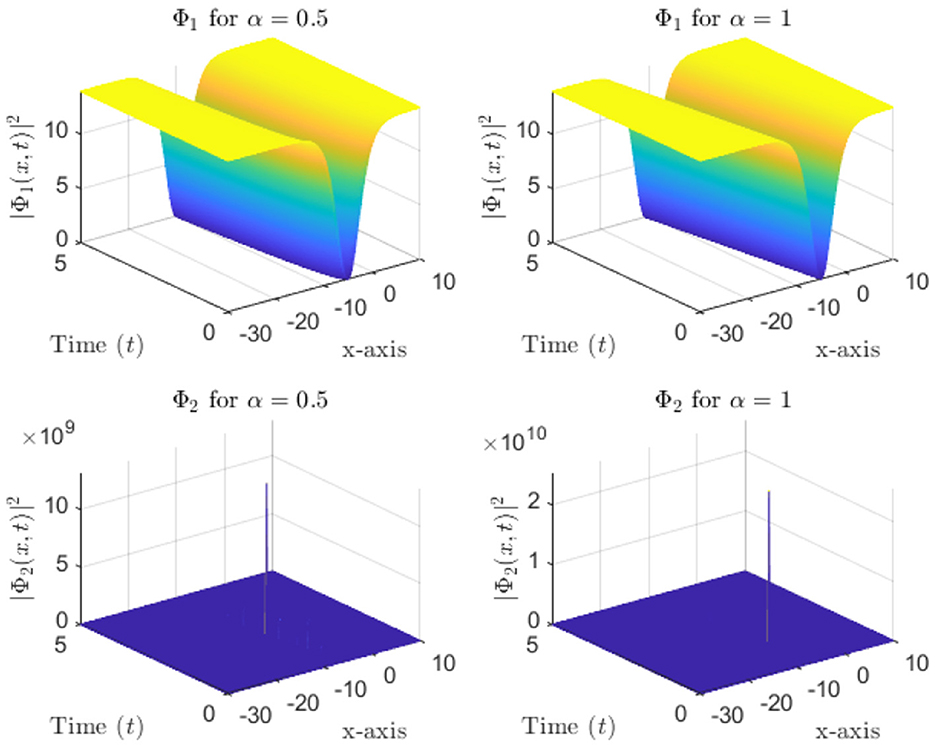
Figure 1. 3D soliton intensity plots of $|{\Phi }_1\left(x,t\right){|}^2$ (tanh profile) and $|{\Phi }_2\left(x,t\right){|}^2$ (coth profile) for Various α values. (Top row), $|{\Phi }_1\left(x,t\right){|}^2$, (Bottom row), $|{\Phi }_2\left(x,t\right){|}^2$.

Figure 2

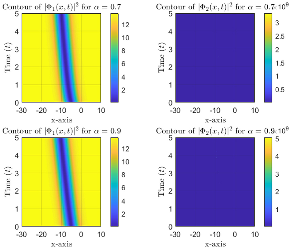
Figure 2. Contour plots of soliton intensity $|{\Phi }_1{|}^2$ and $|{\Phi }_2{|}^2$ for different α values, showing spatial and temporal evolution.

Figure 3

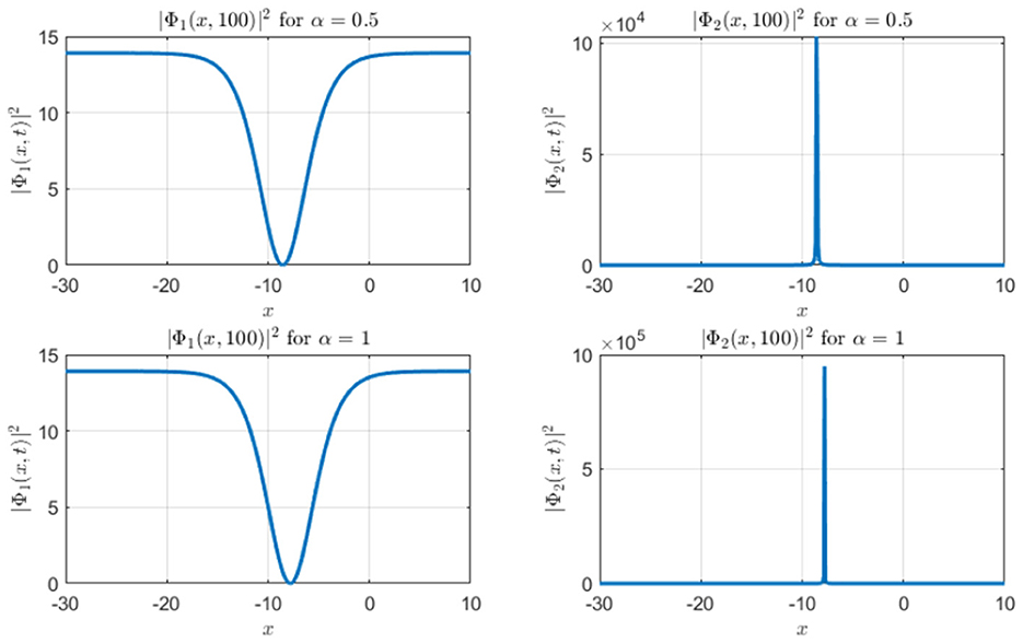
Figure 3. Spatial profiles of soliton intensity $|{\Phi }_1{|}^2$ and $|{\Phi }_2{|}^2$ at fixed time t₀ = 100.

Figure 4

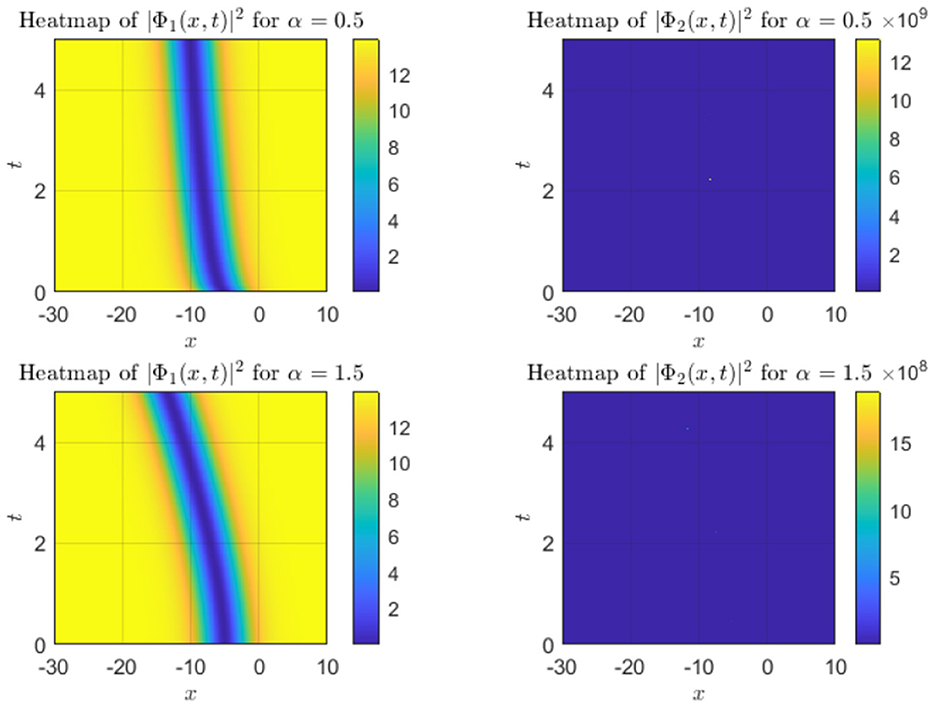
Figure 4. Heatmap visualization of $|{\Phi }_1{|}^2$ and $|{\Phi }_2{|}^2$ for various α values, highlighting intensity distribution over time and space.

Figure 5

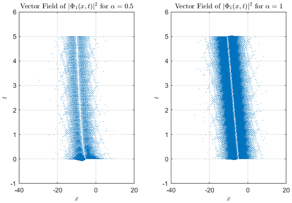
Figure 5. Vector field representation of soliton intensity $|{\Phi }_1{|}^2$ for different α values, depicting gradient flow in space-time.

Figure 6

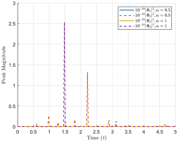
Figure 6. The vertical axis is labeled “Peak Magnitude,” and the horizontal axis is labeled “Time (t).” Peak magnitude evolution of $|{\Phi }_1{|}^2$ and $|{\Phi }_2{|}^2$ over time for various α values.

Figure 7

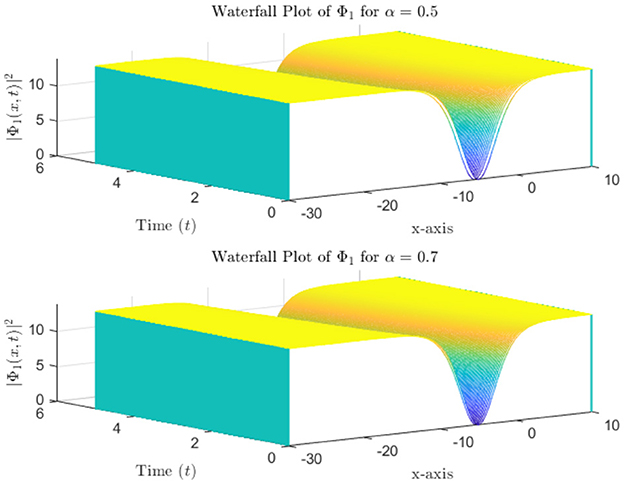
Figure 7. Waterfall plot showing temporal evolution of peak magnitude $|{\Phi }_1{|}^2$ and $|{\Phi }_2{|}^2$ over time.

Figure 8

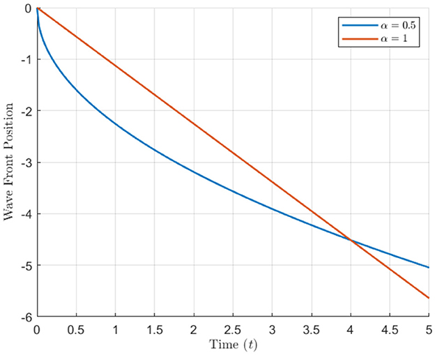
Figure 8. Wave front position as a function of time for different α values, illustrating propagation dynamics.

The real part of the soliton wave function is visualized in Figure 9. The oscillatory nature of the Φ₁ wave is apparent, while Φ₂ exhibits significantly more localized peaks. This figure highlights the contrast between the oscillatory pattern of Φ₁ and the sharply localized nature of Φ₂, underscoring the distinct phase behavior governed by the hyperbolic functions. Figure 10 presents soliton profiles at a fixed time, allowing for direct comparison between different α values. As α increases, the solitons become more localized and sharper. This time-slice comparison highlights the impact of α on soliton shape and spatial extent. Figure 11 presents cross-sectional views of soliton intensity profiles for various α values.

Figure 9

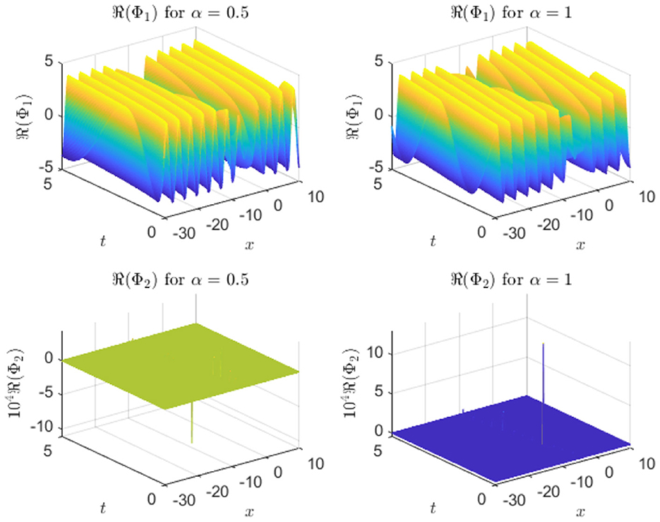
Figure 9. Real part of soliton wave function |Φ(x, t)| over time for various α values.

Figure 10

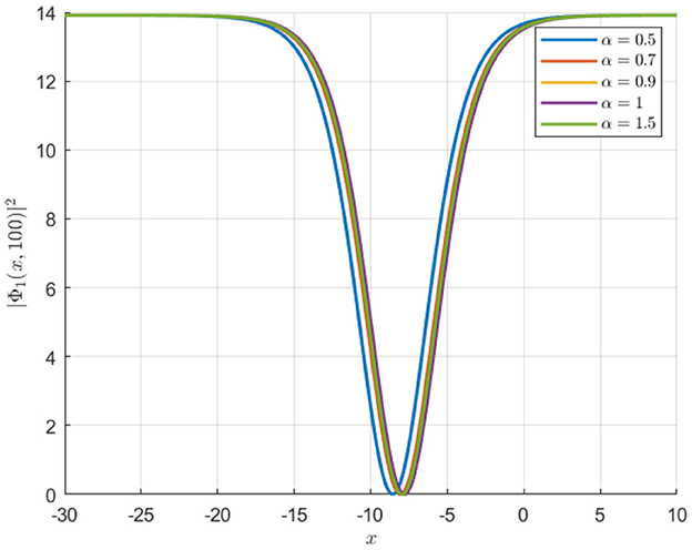
Figure 10. Soliton profiles at fixed time, demonstrating the effect of α on soliton shape.

Figure 11

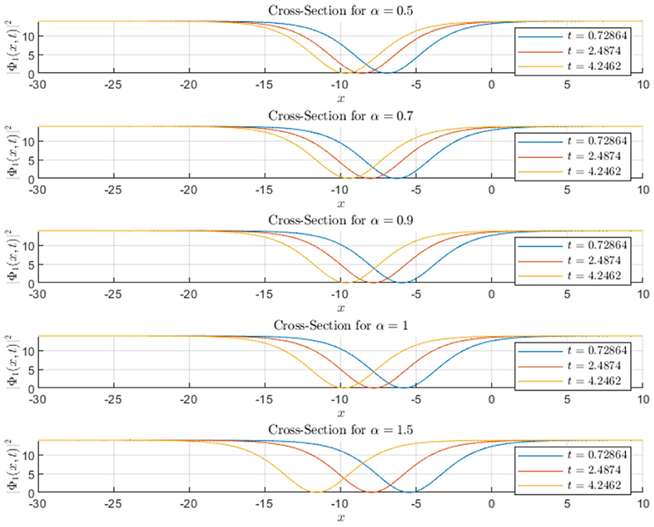
Figure 11. Cross-sectional view of soliton intensity |Φ(x, t)|² for different α values.

The pronounced localization and peak amplitude of Φ₂ indicate reduced dispersion relative to Φ₁. This comparison highlights the differential spreading characteristics driven by soliton type and α variations. Additionally, Figure 12 illustrates the full temporal evolution of the soliton waves.

Figure 12

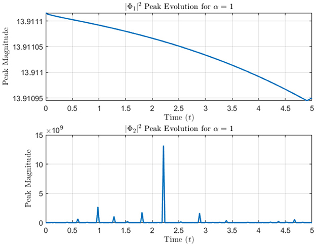
Figure 12. Temporal evolution of soliton wave |Φ(x, t)| over time, showing propagation dynamics for different α values.

The gradual propagation of Φ₁ is contrasted with the sharp, distinct peaks of Φ₂, further reflecting their unique soliton structures and temporal dynamics.

The soliton solutions Φ₁ through Φ₁₀ are classified based on the sign of the Riccati parameter γ₀, which determines the functional form of the solutions to the auxiliary equation ${\chi }^{\prime }\left(\xi \right)={\chi }^2+{\gamma }_0$. Specifically, when γ₀ < 0, the solutions involve hyperbolic functions (e.g. tanh, coth), and when γ₀ > 0, they involve trigonometric functions (e.g. tan, cot). The subsequent set of solutions Φ₁₁ to Φ₂₀ is obtained by solving an alternative branch of the algebraic system arising from the modified simplest equation method. Although this second case introduces different values for the algebraic parameters ρ_i, β₀, and β₁, classification into trigonometric or hyperbolic types remains strictly governed by the sign of γ₀. Hence, Φ₁₁-Φ₁₅ correspond to γ₀ < 0, and Φ₁₆-Φ₂₀ correspond to γ₀ > 0. This clarification is provided to avoid confusion: the division into cases is determined by the structure of the differential equation (through γ₀), not by the values of the algebraic coefficients themselves.

4.2 Solution of the system: second case

The coefficients ϱ₃, ϱ₄, β₀, and β₁ are given by the following expressions:

$\begin{array}{l}{\varrho }_3=\frac{\begin{array}{c}-24{\varrho }_1{\gamma }_0^2{\varrho }_6-4{\varrho }_7{\varrho }_2{\gamma }_0-{\varrho }_7{\varrho }_6\\ +\sqrt{-(4{\varrho }_7{\varrho }_5-{\varrho }_6^2){(24{\varrho }_1{\gamma }_0^2-{\varrho }_7)}^2}\end{array}}{2{\varrho }_7{\gamma }_0},\\ {\varrho }_4=\frac{\begin{array}{c}(-4{\varrho }_1{\gamma }_0^2+{\varrho }_7)\sqrt{-(4{\varrho }_7{\varrho }_5-{\varrho }_6^2){(24{\varrho }_1{\gamma }_0^2-{\varrho }_7)}^2}\\ +96{\gamma }_0\left({\varrho }_1{\gamma }_0{\varrho }_6+\frac{{\varrho }_7{\varrho }_2}{2}\right)\left({\varrho }_1{\gamma }_0^2-\frac{{\varrho }_7}{24}\right)\end{array}}{\begin{array}{c}{\gamma }_0(24{\varrho }_1{\gamma }_0^2{\varrho }_6-{\varrho }_6{\varrho }_7-\\ \sqrt{-(4{\varrho }_7{\varrho }_5-{\varrho }_6^2){(24{\varrho }_1{\gamma }_0^2-{\varrho }_7)}^2})\end{array}},\\ {\beta }_0=0,\\ {\beta }_1=\frac{\begin{array}{c}(-2{\gamma }_0(-24{\varrho }_1{\gamma }_0^2{\varrho }_6+{\varrho }_7{\varrho }_6\\ +\sqrt{-(4{\varrho }_7{\varrho }_5-{\varrho }_6^2){(24{\varrho }_1{\gamma }_0^2-{\varrho }_7)}^2}\left){\varrho }_7\right(24{\varrho }_1{\gamma }_0^2-{\varrho }_7){)}^{\frac{1}{2}}\end{array}}{\begin{array}{c}{\gamma }_0(-24{\varrho }_1{\gamma }_0^2{\varrho }_6+{\varrho }_7{\varrho }_6\\ +\sqrt{-(4{\varrho }_7{\varrho }_5-{\varrho }_6^2){(24{\varrho }_1{\gamma }_0^2-{\varrho }_7)}^2})\end{array}}.& (18)\end{array}$

Utilizing Equations 3, 8, 14, and 15, we obtain the following optical solutions:

$\begin{array}{l}{\Phi }_{11}\left(x,t\right)={\beta }_1\sqrt{-{\gamma }_0}tanh\left(\sqrt{-{\gamma }_0}\left(h\left(x-\frac{{\lambda }_1{t}^{\alpha }}{\alpha }\right)+s\right)\right)\end{array}$

$\begin{array}{ll}{e}^{i\left(-kx+\frac{w{t}^{\alpha }}{\alpha }+\varphi \right)},& (19)\end{array}$

$\begin{array}{l}{\Phi }_{12}\left(x,t\right)={\beta }_1\sqrt{-{\gamma }_0}coth\left(\sqrt{-{\gamma }_0}\left(h\left(x-\frac{{\lambda }_1{t}^{\alpha }}{\alpha }\right)+s\right)\right)\end{array}$

$\begin{array}{ll}{e}^{i\left(-kx+\frac{w{t}^{\alpha }}{\alpha }+\varphi \right)},& (20)\end{array}$

$\begin{array}{l}{\Phi }_{13}\left(x,t\right)={\beta }_1\sqrt{-{\gamma }_0}(-tanh\left(2\sqrt{-{\gamma }_0}\left(h\left(x-\frac{{\lambda }_1{t}^{\alpha }}{\alpha }\right)+s\right)\right)\\ +isech\left(2\sqrt{-{\gamma }_0}\left(h\left(x-\frac{{\lambda }_1{t}^{\alpha }}{\alpha }\right)+s\right)\right)\end{array}$

$\begin{array}{ll}{e}^{i\left(-kx+\frac{w{t}^{\alpha }}{\alpha }+\varphi \right)},& (21)\end{array}$

$\begin{array}{ll}{\Phi }_{14}\left(x,t\right)={\beta }_1\sqrt{-{\gamma }_0}(-coth\left(2\sqrt{-{\gamma }_0}\left(h\left(x-\frac{{\lambda }_1{t}^{\alpha }}{\alpha }\right)+s\right)\right)& (22)\end{array}$

$\begin{array}{l}+csch\left(2\sqrt{-{\gamma }_0}\left(h\left(x-\frac{{\lambda }_1{t}^{\alpha }}{\alpha }\right)+s\right)\right))\\ e^{i\left(-kx+\frac{w{t}^{\alpha }}{\alpha }+\varphi \right)},\end{array}$

$\begin{array}{ll}{\Phi }_{15}\left(x,t\right)={\beta }_1\sqrt{-{\gamma }_0}(tanh\left(\frac{\sqrt{-{\gamma }_0}}{2}\left(h\left(x-\frac{{\lambda }_1{t}^{\alpha }}{\alpha }\right)+s\right)\right)& (23)\end{array}$

$\begin{array}{l}+coth\left(\frac{\sqrt{-{\gamma }_0}}{2}\left(h\left(x-\frac{{\lambda }_1{t}^{\alpha }}{\alpha }\right)+s\right)\right))\\ e^{i\left(-kx+\frac{w{t}^{\alpha }}{\alpha }+\varphi \right)}.\end{array}$

Additionally, applying Equations 3, 8, 14, 15, and 18 yields the following optical solutions:

$\begin{array}{l}{\Phi }_{16}\left(x,t\right)={\beta }_1\sqrt{{\gamma }_0}tan\left(\sqrt{{\gamma }_0}\left(h\left(x-\frac{{\lambda }_1{t}^{\alpha }}{\alpha }\right)+s\right)\right)\end{array}$

$\begin{array}{ll}{e}^{i\left(-kx+\frac{w{t}^{\alpha }}{\alpha }+\varphi \right)},& (24)\end{array}$

$\begin{array}{l}{\Phi }_{17}(x,t)={\beta }_1\sqrt{{\gamma }_0}\cot \left(\sqrt{{\gamma }_0}\left(h\left(x-\frac{{\lambda }_1{t}^{\alpha }}{\alpha }\right)+s\right)\right)\\ e^{i\left(-kx+\frac{w{t}^{\alpha }}{\alpha }+\varphi \right)},& (25)\end{array}$

$\begin{array}{l}{\Phi }_{18}(x,t)={\beta }_1\sqrt{{\gamma }_0}(-\tan \left(2\sqrt{{\gamma }_0}\left(h\left(x-\frac{{\lambda }_1{t}^{\alpha }}{\alpha }\right)+s\right)\right)\\ +\sec \left(2\sqrt{{\gamma }_0}\left(h\left(x-\frac{{\lambda }_1{t}^{\alpha }}{\alpha }\right)+s\right)\right))\\ e^{i(-kx+\frac{w{t}^{\alpha }}{\alpha }+\varphi )},& (26)\end{array}$

$\begin{array}{l}{\Phi }_{19}(x,t)={\beta }_1\sqrt{{\gamma }_0}(-\cot \left(2\sqrt{{\gamma }_0}\left(h\left(x-\frac{{\lambda }_1{t}^{\alpha }}{\alpha }\right)+s\right)\right)\\ +\csc \left(2\sqrt{{\gamma }_0}\left(h\left(x-\frac{{\lambda }_1{t}^{\alpha }}{\alpha }\right)+s\right)\right))e^{i(-kx+\frac{w{t}^{\alpha }}{\alpha }+\varphi )},& (27)\end{array}$

$\begin{array}{l}{\Phi }_{20}(x,t)={\beta }_1\sqrt{{\gamma }_0}(\tan \left(\frac{\sqrt{{\gamma }_0}}{2}\left(h\left(x-\frac{{\lambda }_1{t}^{\alpha }}{\alpha }\right)+s\right)\right)\\ +\cot \left(\frac{\sqrt{{\gamma }_0}}{2}\left(h\left(x-\frac{{\lambda }_1{t}^{\alpha }}{\alpha }\right)+s\right)\right))\\ e^{i(-kx+\frac{w{t}^{\alpha }}{\alpha }+\varphi )}.& (28)\end{array}$

The following figures present various aspects of soliton solutions Φ₁₁(x, t) for two different values of the fractional-order parameter α = 0.5 and α = 1.5. The simulations are based on the following parameters:

$\begin{array}{lll}a=-0.9,& b=0.2,& w=2,\\ {\tau }_1=0.1,& {\tau }_3=0.1,& {\tau }_4=0.5,\\ {\tau }_5=0.5,& {\tau }_6=0.5,& {\tau }_7=0.7,\\ {\tau }_8=1,& {\tau }_9=2,& h=0.1,\\ c_1=0.1,& c_2=0.1,& {\gamma }_0=-10,\\ \varphi =0.1,& s=0.5.\end{array}$

The results are presented for different values of the fractional order parameter α.

The figures provide a comparative analysis of soliton intensity, spatial profiles, peak magnitudes, and wave front dynamics. The results demonstrate the influence of varying α on the dynamics and shape of the solitons. As shown in Figure 13, the soliton intensity $|{\Phi }_{11}\left(x,t\right){|}^2$ varies with α. For α = 0.5, the soliton maintains a broader profile, indicating slower propagation. In contrast, at α = 1.5, the soliton exhibits a sharper, faster-evolving profile. Figure 14 highlights the spatial profile of Φ₁₁ at a fixed time. The soliton for α = 1.5 is narrower and shifts forward compared to α = 0.5. This indicates that higher α accelerates the soliton's evolution and alters its spatial localization. Figure 15 shows how the peak magnitude evolves over time. For α = 0.5, the peak stabilizes slowly, while for α = 1.5, the soliton reaches its peak faster. This reflects the faster temporal evolution of solitons at higher α. Figure 16 illustrates the propagation of the soliton wave front over time. For α = 1.5, the wave front progresses more rapidly compared to α = 0.5, indicating enhanced soliton mobility and faster response to perturbations. These results demonstrate that the fractional parameter α significantly affects the soliton's propagation speed, spatial profile, and peak intensity. Higher values of α lead to faster, more localized solitons, while lower α values result in broader, slower-moving solitons.

Figure 13

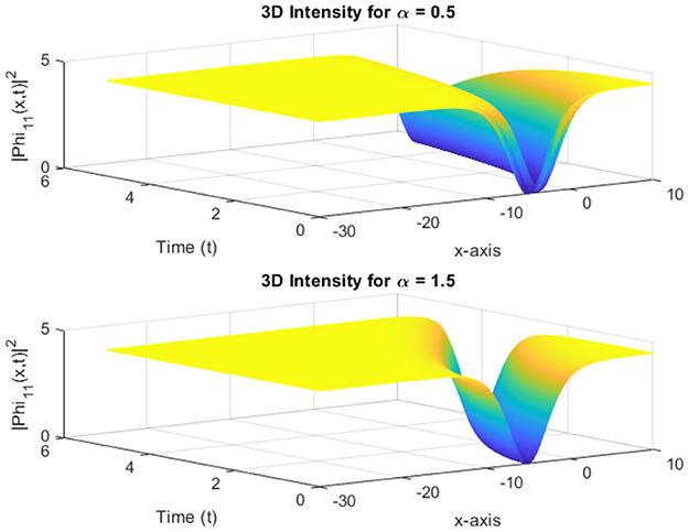
Figure 13. 3D Soliton intensity plots of $|{\Phi }_{11}\left(x,t\right){|}^2$ (tanh profile) for various α values.

Figure 14

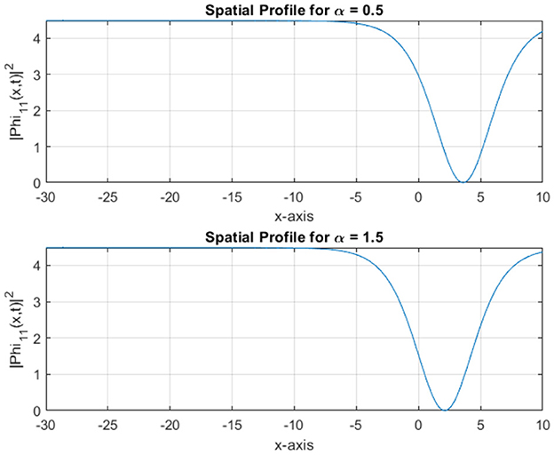
Figure 14. Spatial profile of Φ₁₁(x, t) at a fixed time.

Figure 15

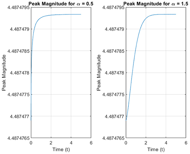
Figure 15. Peak magnitude evolution of $|{\Phi }_{11}\left(x,t\right){|}^2$ over time.

Figure 16

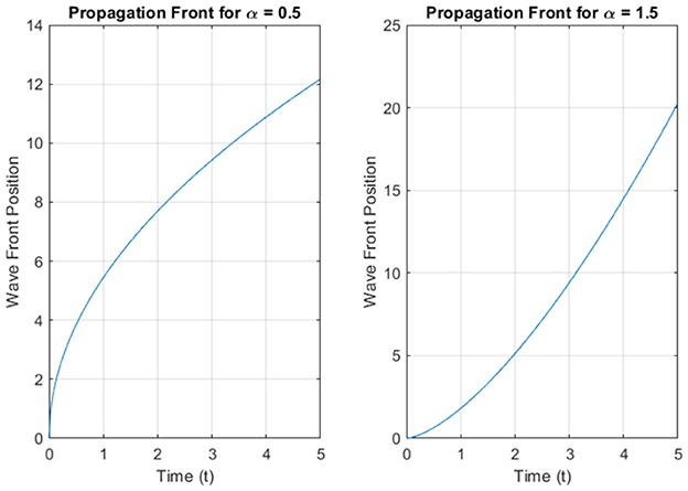
Figure 16. Wave front position over time for Φ₁₁(x, t).

5 Application of the Kudryashov method

5.1 Kudryashov method

The Kudryashov method is a powerful and efficient analytical approach for deriving exact solutions to nonlinear differential equations, particularly in the context of soliton theory and wave propagation [43]. This method has been widely applied to nonlinear evolution equations, offering explicit forms of soliton solutions that are crucial for understanding complex dynamical systems. In this section, we employ the Kudryashov method to obtain new conformable optical soliton solutions for the concatenated nonlinear model, providing deeper insights into the propagation of solitons in optical fibers.

The Kudryashov method is a systematic approach for deriving exact solutions to nonlinear differential equations. The process begins by formulating the governing nonlinear equation and applying a traveling wave transformation, typically $\xi =h\left(x-\frac{v{t}^{\alpha }}{\alpha }\right)$, to reduce the partial differential equation (PDE) to an ordinary differential equation (ODE). An ansatz is then assumed for the solution, often in the form $\Phi \left(\xi \right)={\eta }_0+\sum _{i=1}^N{\eta }_i{\chi }^i\left(\xi \right)$, where χ(ξ) is a known function, such as a hyperbolic or trigonometric function. To determine the expansion degree N, the balancing principle is applied, equating the highest-order derivative term with the dominant nonlinear term in the equation. The assumed solution is substituted into the reduced ODE, leading to a polynomial equation in terms of χ(ξ). By collecting like terms and setting the coefficients of each power of χ(ξ) to zero, a system of algebraic equations is obtained. Solving this system provides the unknown constants (η_i, k, etc.), which are then used to construct the explicit soliton solutions. These solutions are further analyzed and visualized to examine soliton dynamics, stability, and propagation characteristics. The method also allows for the evaluation of physical properties such as energy, peak intensity, and interaction behaviors, offering deeper insights into the complex dynamics of soliton systems.

The following solution, applicable to this model, is adopted from [44]:

$\begin{array}{ll}\chi \left(\xi \right)=\frac{1}{\left(c_1-c_2\right)sinh\left(\xi \right)+\left(c_1+c_2\right)cosh\left(\xi \right)},& (29)\end{array}$

where c₁ and c₂ are arbitrary constants that can be tuned to satisfy the boundary conditions and the constraints of the governing nonlinear equation. This function represents a general form of solitary wave solutions that exhibit localized behavior over an extended spatial domain [45]. The function χ(ξ) satisfies the following fundamental relation:

$\begin{array}{ll}{\left(\frac{d\chi \left(\xi \right)}{d\xi }\right)}^2=\chi {\left(\xi \right)}^2\left(1-4c_1{c}_2\chi {\left(\xi \right)}^2\right).& (30)\end{array}$

Equation 30 highlights the nonlinearity inherent in the system, which governs the shape and amplitude of solitons. This quadratic relationship implies that the soliton amplitude is influenced by the interaction between the coefficients c₁ and c₂, making it possible to control the soliton profile through these adjustable parameters.

To construct explicit soliton solutions to Equation 9, we adopt the following series representation using the Kudryashov approach:

$\begin{array}{ll}\Phi \left(\xi \right)={\eta }_0+{\displaystyle \sum _{i=1}^N}{\eta }_i\chi {\left(\xi \right)}^i,& (31)\end{array}$

where η₀, η₁, …, η_N are unknown constants that need to be determined. The parameter N denotes the highest power of χ(ξ) in the series expansion and is determined by balancing the highest-order derivative term and the nonlinear term in the governing equation. This series form enables the extraction of various soliton profiles by solving a system of algebraic equations for the coefficients η_i.

This procedure results in a system of algebraic equations as follows:

$\begin{array}{ll}\begin{array}{l}{\left(\chi \left(\xi \right)\right)}^0:384c_1^2{c}_2^2{\rho }_1{\beta }_1-8c_1{c}_2{\rho }_2{\beta }_1^3-4c_1{c}_2{\rho }_3{\beta }_1^3+{\rho }_5{\beta }_1^5=0,\\ {\left(\chi \left(\xi \right)\right)}^1:-16c_1{c}_2{\rho }_2{\beta }_0{\beta }_1^2-4c_1{c}_2{\rho }_3{\beta }_0{\beta }_1^2+5{\rho }_5{\beta }_0{\beta }_1^4=0,\\ {\left(\chi \left(\xi \right)\right)}^2:-8c_1{c}_2{\rho }_2{\beta }_0^2{\beta }_1+10{\rho }_5{\beta }_0^2{\beta }_1^3-8c_1{c}_2{\rho }_1{\beta }_1-8c_1{c}_2{\rho }_1{\beta }_1\\ +\left({\rho }_2+{\rho }_3+{\rho }_6\right){\beta }_1^3=0,\\ {\left(\chi \left(\xi \right)\right)}^3:10{\rho }_5{\beta }_0^3{\beta }_1^2+2{\rho }_2{\beta }_0{\beta }_1^2+{\rho }_3{\beta }_0{\beta }_1^2+3{\rho }_6{\beta }_0{\beta }_1^2=0,\\ {\left(\chi \left(\xi \right)\right)}^4:5{\rho }_5{\beta }_0^4{\beta }_1+{\rho }_2{\beta }_0^2{\beta }_1+3{\rho }_6{\beta }_0^2{\beta }_1+\left({\rho }_1+{\rho }_4+{\rho }_7\right){\beta }_1=0,\\ {\left(\chi \left(\xi \right)\right)}^5:{\rho }_5{\beta }_0^5+{\rho }_6{\beta }_0^3+{\rho }_7{\beta }_0=0.\end{array}& (32)\end{array}$

Once again, two cases can be considered. First case: The solutions to the above system are given by:

$\begin{array}{l}{\rho }_1=-{\rho }_4-{\rho }_7,\\ {\rho }_5=\frac{\begin{array}{c}3\left(\left(-{\rho }_2+\frac{{\rho }_3}{2}+2{\rho }_6\right){\rho }_4+4{\rho }_7\left(-{\rho }_2+\frac{{\rho }_3}{3}+\frac{3{\rho }_6}{2}\right)\right)\\ \left({\rho }_2+{\rho }_3+{\rho }_6\right)\end{array}}{{(9{\rho }_4+10{\rho }_7)}^2},\\ {\beta }_0=0,\\ {\beta }_1=-\frac{2\sqrt{-2\left({\rho }_2+{\rho }_3+{\rho }_6\right)c_1{c}_2\left(9{\rho }_4+10{\rho }_7\right)}}{{\rho }_2+{\rho }_3+{\rho }_6}.& (33)\end{array}$

Using Equations 4, 5, 8, and 33, the following optical solutions are derived

$\begin{array}{l}{\Phi }_{21}(x,t)=\frac{{\beta }_1{e}^{i\left(-kx+\frac{w{t}^{\alpha }}{\alpha }+\varphi \right)}}{\begin{array}{c}(c_1-c_2)\sinh \left(h\left(x-\frac{{\lambda }_1{t}^{\alpha }}{\alpha }\right)\right)\\ +(c_1+c_2)\cosh \left(h\left(x-\frac{{\lambda }_1{t}^{\alpha }}{\alpha }\right)\right)\end{array}},\\ {\Phi }_{22}(x,t)=\frac{{\beta }_1}{2c_2}\text{ sech}\left(h\left(x-\frac{{\lambda }_1{t}^{\alpha }}{\alpha }\right)\right)e^{i\left(-kx+\frac{w{t}^{\alpha }}{\alpha }+\varphi \right)},\\ {\Phi }_{23}(x,t)=-\frac{{\beta }_1}{2c_2}\text{csch}\left(h\left(x-\frac{{\lambda }_1{t}^{\alpha }}{\alpha }\right)\right)e^{i\left(-kx+\frac{w{t}^{\alpha }}{\alpha }+\varphi \right)}.& (34)\end{array}$

A second case can be considered: The solutions to the algebraic system yield the following expressions:

$\begin{array}{l}{\rho }_4=-{\rho }_7-{\rho }_1,\\ {\rho }_5=\frac{3\left({\rho }_6+{\rho }_2+{\rho }_3\right)\left(\left({\rho }_2-\frac{{\rho }_3}{2}-2{\rho }_6\right){\rho }_1-{\rho }_7\left({\rho }_2+\frac{{\rho }_3}{3}\right)\right)}{{(9{\rho }_1-{\rho }_7)}^2},\\ {\beta }_0=0,\\ {\beta }_1=\frac{2\sqrt{2\left({\rho }_6+{\rho }_2+{\rho }_3\right)c_1{c}_2\left(9{\rho }_1-{\rho }_7\right)}}{{\rho }_6+{\rho }_2+{\rho }_3}.& (35)\end{array}$

Utilizing Equations 4, 5, 8, and 35, the following optical solutions are derived:

$\begin{array}{l}{\Phi }_{24}(x,t)=\frac{{\beta }_1{e}^{i\left(-kx+\frac{w{t}^{\alpha }}{\alpha }+\varphi \right)}}{\begin{array}{c}(c_1-c_2)\sinh \left(h\left(x-\frac{{\lambda }_1{t}^{\alpha }}{\alpha }\right)\right)\\ +(c_1+c_2)\cosh \left(h\left(x-\frac{{\lambda }_1{t}^{\alpha }}{\alpha }\right)\right)\end{array}},\\ {\Phi }_{25}(x,t)=\frac{{\beta }_1}{2c_2}\text{ sech}\left(h\left(x-\frac{{\lambda }_1{t}^{\alpha }}{\alpha }\right)\right)e^{i\left(-kx+\frac{w{t}^{\alpha }}{\alpha }+\varphi \right)},\\ {\Phi }_{26}(x,t)=-\frac{{\beta }_1}{2c_2}\text{csch}\left(h\left(x-\frac{{\lambda }_1{t}^{\alpha }}{\alpha }\right)\right)e^{i\left(-kx+\frac{w{t}^{\alpha }}{\alpha }+\varphi \right)}.& (36)\end{array}$

5.2 Visualization and analysis of soliton dynamics

Figure 17 displays the time evolution of $|{\Phi }_{24}\left(x,t\right){|}^2$ for four distinct time slices (t = 1, 3, 5, 7). The soliton maintains a smooth bell-shaped profile as it propagates in the positive x-direction. The peak intensity gradually decreases, and the soliton broadens slightly over time, indicating a stable, spreading wave. The curve shifts rightward, highlighting the directional propagation of the wave. Figure 18 illustrates the evolution of $|{\Phi }_{25}\left(x,t\right){|}^2$, where the soliton retains a bright, localized peak as it propagates. The peak remains nearly constant in intensity, a characteristic of bright solitons. Over time, the soliton maintains its structure while moving along the positive x-axis, demonstrating its robustness and stability. Figure 19 presents the evolution of $|{\Phi }_{26}\left(x,t\right){|}^2$, which features sharp peaks caused by the singularity of the csch function. The soliton exhibits high-intensity spikes at different time steps, with the peaks shifting rightward as time progresses. The peak intensities are significantly larger compared to Φ₂₄ and Φ₂₅, highlighting the soliton's distinct singular nature. Figure 20 illustrates the logarithmic peak intensity evolution of the soliton solutions Φ₂₄, Φ₂₅, and Φ₂₆ over time. All the figures presented were generated using the parameter values listed in Table 1.

Figure 17

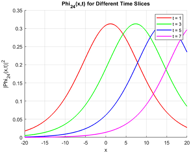
Figure 17. Temporal evolution of $|{\Phi }_{24}\left(x,t\right){|}^2$ at different time slices.

Figure 18

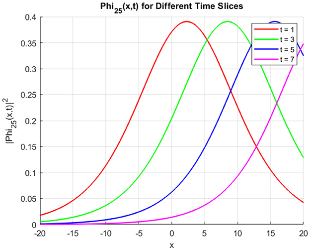
Figure 18. Temporal evolution of $|{\Phi }_{25}\left(x,t\right){|}^2$ at different time slices.

Figure 19

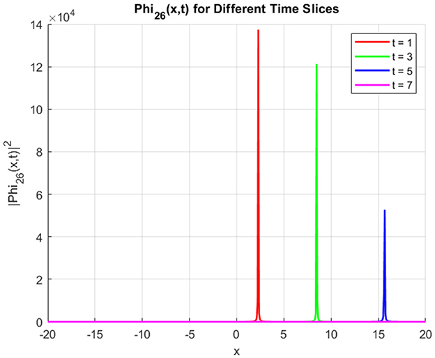
Figure 19. Temporal evolution of $|{\Phi }_{26}\left(x,t\right){|}^2$ at different time slices.

Figure 20

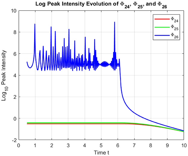
Figure 20. Log peak intensity evolution of Φ₂₄, Φ₂₅, and Φ₂₆ over time.

Table 1

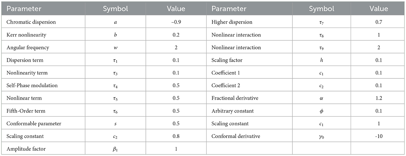
Table 1. Parameters used to generate all figures in the Kudryashov method, including the log peak intensity plot.

The soliton solutions Φ₂₄ and Φ₂₅ maintain stable peak intensities throughout their evolution, exhibiting only minimal decay over time. This behavior highlights their inherent stability as soliton structures, making them resilient to dispersive and nonlinear effects. In contrast, Φ₂₆ displays pronounced high-intensity spikes and irregular fluctuations, a hallmark of singular solutions driven by the hyperbolic cosecant function embedded in its formulation. These sharp intensity variations reflect its susceptibility to rapid amplitude changes. Notably, after t = 6, Φ₂₆ experiences a rapid decay in energy, leading to a transition into a lower energy state. This post-peak energy loss further emphasizes the transient and unstable nature of Φ₂₆ compared to the more stable profiles of Φ₂₄ and Φ₂₅.

5.3 Multi-soliton interactions and collisions

We analyzed the structural relationships in soliton interactions and examined their properties. This part delves into the interaction dynamics between two distinct soliton solutions, namely the Sech-based soliton Φ₂₅ and the Csch-based soliton Φ₂₆, derived using the Kudryashov method. These soliton solutions exhibit distinct characteristics: Φ₂₅ is known for its localized and stable bell-shaped profile, while Φ₂₆ introduces a singular behavior due to its hyperbolic cosecant structure [46].

The interaction between solitons is modeled here via linear superposition of two exact solutions (Φ₂₅ and Φ₂₆). While this approach does not yield a true multi-soliton solution, it offers a tractable approximation for non-integrable systems. Notably, Equation 1 contains non-variational terms involving Φ^*, precluding a Lagrangian formulation and thus the use of action-based interaction analysis. The superposition method is therefore used as a qualitative tool to capture essential features of soliton dynamics such as amplitude modulation and energy redistribution.

The combined soliton solution for the multi-soliton interaction is constructed by superimposing the two solitons:

$\begin{array}{ll}{\Phi }_{\text{total}}\left(x,t\right)={\Phi }_{25}\left(x,t\right)+{\Phi }_{26}\left(x,t\right),& (37)\end{array}$

where

$\begin{array}{ll}{\Phi }_{25}\left(x,t\right)=\frac{{\beta }_1}{2c_2}\text{ sech}\left(h\left(x-\frac{{\lambda }_1{t}^{\alpha }}{\alpha }\right)\right)e^{i\left(-kx+\frac{w{t}^{\alpha }}{\alpha }+\varphi \right)},& (38)\end{array}$

and

$\begin{array}{ll}{\Phi }_{26}\left(x,t\right)=-\frac{{\beta }_1}{2c_2}\text{csch}\left(h\left(x-\frac{{\lambda }_1{t}^{\alpha }}{\alpha }\right)\right)e^{i\left(-kx+\frac{w{t}^{\alpha }}{\alpha }+\varphi \right)}.& (39)\end{array}$

The interaction between Φ₂₅ and Φ₂₆ reveals complex dynamics driven by the interplay of the hyperbolic secant and cosecant functions, leading to energy exchange, intensity fluctuations, and non-trivial collision behavior.

Figure 21 presents the log₁₀ contour plot of the combined soliton interaction over time and space. The color gradient effectively visualizes the soliton trajectories and intensity variations. The Sech-based soliton (Φ₂₅) contributes a smooth, bell-shaped trajectory, while the Csch-based soliton (Φ₂₆) introduces sharp gradients and localized spikes due to its singular nature.

Figure 21

Figure 21. log₁₀ Contour plot of multi-soliton interaction between Φ₂₅ and Φ₂₆. The plot highlights the evolution of soliton intensities and their propagation paths over time.

The contour plot illustrates the propagation of solitons over the spatial domain, with visible energy exchanges during interactions. High-intensity regions are marked in warmer colors, while regions of lower intensity are displayed in cooler tones. The log scale enhances the visualization of both strong and weak intensity regions.

To further analyze the interaction dynamics, Figure 22 displays the evolution of the peak intensity over time on a logarithmic scale. The plot captures the oscillatory behavior of the intensity peaks, reflecting energy fluctuations during the interaction process. The logarithmic scale highlights subtle variations and abrupt intensity spikes. The observed fluctuations are characteristic of the interaction between stable and singular soliton structures, where transient energy surges occur at collision points.

Figure 22

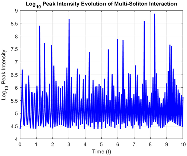
Figure 22. log₁₀ Peak intensity evolution of the multi-soliton interaction. Fluctuations indicate energy exchange and dynamic interactions between Φ₂₅ and Φ₂₆.

To provide a clearer and more concise understanding of soliton evolution, Figure 23 presents intensity profiles at specific time slices, revealing how the spatial structures of the solitons Φ₂₅ and Φ₂₆ evolve during their interaction. These snapshots depict the dynamic nature of the soliton profiles, showcasing key phenomena such as energy exchange, stability, and collision dynamics. The interaction between the sech-based soliton Φ₂₅ and the csch-based soliton Φ₂₆ demonstrates transient energy redistribution, where peak intensities undergo periodic amplification and suppression.

Figure 23

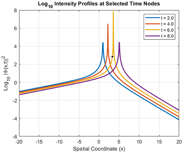
Figure 23. Soliton intensity profiles at selected time nodes, illustrating the evolution and collision dynamics of Φ₂₅ and Φ₂₆ during interaction.

Notably, Φ₂₅ retains structural stability despite the interaction, while Φ₂₆ exhibits significant fluctuations due to its inherent singular characteristics. During collision events, sharp intensity spikes are observed, followed by the gradual restoration of each soliton's original profile, reflecting the hallmark elastic behavior of soliton interactions. The contrasting behaviors of these two soliton types result in complex nonlinear dynamics. Φ₂₅ displays localized energy concentration and stable propagation, making it ideal for applications that demand signal consistency. In contrast, Φ₂₆ undergoes rapid intensity shifts and strong localization effects, which are commonly observed in singular soliton dynamics and have implications in fields such as plasma physics and hydrodynamics.

The logarithmic intensity analysis provides deeper insight into both dominant and subtle features, capturing energy fluctuations across strong and weak regions within the system.

To quantify these interactions, the total energy of the system is computed using the expression:

$E\left(t\right)={\displaystyle {\int }_{-\infty }^{\infty }}|{\Phi }_{25}\left(x,t\right)+{\Phi }_{26}\left(x,t\right){|}^{2}dx,$

where Φ₂₅(x, t) and Φ₂₆(x, t) represent the individual soliton waveforms, and |Φ(x, t)|² corresponds to the soliton intensity. Expanding the square modulus gives:

$\begin{array}{l}E\left(t\right)={\displaystyle {\int }_{-\infty }^{\infty }}(|{\Phi }_{25}\left(x,t\right){|}^2+|{\Phi }_{26}\left(x,t\right){|}^2\\ +2\Re \left[{\Phi }_{25}\left(x,t\right){\Phi }_{26}^{*}\left(x,t\right)\right])dx,\end{array}$

where the total energy includes contributions from each soliton and an interaction term reflecting interference effects. The energy dynamics were calculated numerically using the trapezoidal rule for spatial integration, with the results plotted over time on a logarithmic scale (log₁₀) to highlight fluctuations and ensure clear visibility of energy variations. The energy evolution, illustrated in Figure 24, reveals distinct patterns for the two solitons. The Sech-based soliton Φ₂₅ maintains a stable energy profile, indicating its robustness against interaction-induced perturbations. In contrast, the Csch-based soliton Φ₂₆ undergoes frequent energy spikes and fluctuations, a direct consequence of its singular nature. Despite these localized changes, the total energy of the system remains largely conserved, adhering to the principles of integrable systems where energy conservation is a fundamental characteristic. This conservation persists even during intense soliton interactions, underscoring the stability of the system. The energy exchange between the solitons highlights how transient redistributions occur without violating global conservation laws. Such behavior is pivotal in understanding energy transfer mechanisms in nonlinear media, with practical applications in optical communication, fluid dynamics, and plasma physics. The combined analysis of intensity evolution and energy dynamics emphasizes the diverse behaviors that arise from the interaction of Sech-based and Csch-based solitons. It also showcases the effectiveness of fractional calculus in modeling complex soliton systems, enabling the accurate depiction of nonlinear interactions, stability considerations, and energy conservation. These insights not only deepen the theoretical understanding of soliton behavior but also pave the way for future explorations in applied fields where soliton dynamics play a critical role.

Figure 24

Figure 24. Energy exchange dynamics between the Sech-based soliton Φ₂₅ and the Csch-based soliton Φ₂₆.

6 Conclusion

This study presents a comprehensive analysis of multi-soliton dynamics within a conformable concatenated nonlinear model, integrating the nonlinear Schrödinger equation (NLSE), the Sasa-Satsuma (SS) equation, and the Lakshmanan-Porsezian-Daniel (LPD) model. Through the application of advanced analytical techniques—specifically, the modified simplest equation method and the Kudryashov approach—a wide array of exact soliton solutions was systematically derived, including bright, dark, and mixed types. These solutions offer valuable insights into the complex interplay between higher-order dispersion and nonlinear effects, which strongly affect soliton stability, propagation dynamics, and spatial evolution in optical fibers.

A key contribution of this research lies in the incorporation of a conformable fractional derivative, which significantly extends the analytical scope of the model. This fractional framework enables precise and accurate modeling of fractional-order dynamics, capturing intricate behaviors such as energy dissipation, temporal evolution, and soliton stability under varying system parameters. The study reveals how small variations in the fractional order significantly alter soliton profiles, peak intensities, and interaction dynamics, thereby enhancing the flexibility and depth of soliton analysis.

The energy dynamics of soliton interactions were also meticulously examined, emphasizing both individual soliton energies and the total system energy. Using numerical integration techniques, it was demonstrated that—despite complex interaction events such as elastic and inelastic collisions—the total energy of the system remains largely conserved. This observation reflects a fundamental property of soliton systems within integrable models, demonstrating that localized fluctuations do not disrupt overall energy conservation. The application of a logarithmic scale in visualizations further confirmed these fluctuations while reinforcing conservation principles.

Numerical simulations validated the analytical solutions and illustrated how temporal and fractional parameters influence soliton dynamics, peak intensities, and propagation behaviors. Comparative analysis between sech- and csch-based solitons revealed rich nonlinear phenomena, including energy exchange, amplitude modulation, and collision-induced structural changes. In particular, the energy stability of sech-based solitons contrasted with the pronounced fluctuations of csch-based solitons, providing valuable insight into the diverse dynamics governing nonlinear wave systems.

The insights gained from this study not only deepen the understanding of nonlinear wave dynamics but also pave the way for the development of next-generation telecommunication systems. The ability to model, predict, and control soliton behavior with high precision holds immense potential to enhance data transmission efficiency, reduce signal degradation, and optimize optical network infrastructures. Ultimately, the integration of fractional calculus into soliton research opens new avenues for the exploration of complex nonlinear systems across diverse scientific fields, including fluid dynamics, plasma physics, and quantum mechanics.

Data availability statement

The original contributions presented in the study are included in the article/supplementary material, further inquiries can be directed to the corresponding author.

Author contributions

CC: Formal analysis, Methodology, Software, Writing – original draft. SA: Investigation, Methodology, Validation, Writing – original draft, Writing – review & editing. DA: Formal analysis, Supervision, Validation, Writing – original draft, Writing – review & editing.

Funding

The author(s) declare that no financial support was received for the research and/or publication of this article.

Conflict of interest

The authors declare that the research was conducted in the absence of any commercial or financial relationships that could be construed as a potential conflict of interest.

Generative AI statement

The author(s) declare that no Gen AI was used in the creation of this manuscript.

Publisher's note

All claims expressed in this article are solely those of the authors and do not necessarily represent those of their affiliated organizations, or those of the publisher, the editors and the reviewers. Any product that may be evaluated in this article, or claim that may be made by its manufacturer, is not guaranteed or endorsed by the publisher.

References

1. Yoshida S. Physics and mathematics behind wave dynamics. In: Synthesis Lectures on Wave Phenomena in the Physical Sciences. Cham, Switzerland: Springer. (2025). doi: 10.1007/978-3-031-60354-9

Crossref Full Text | Google Scholar

2. Chen YQ, Tang YH, Manafian J, Rezazadeh H, Osman MS. Dark wave, rogue wave and perturbation solutions of Ivancevic option pricing model. Nonlinear Dyn. (2021) 105:2539–48. doi: 10.1007/s11071-021-06642-6

Crossref Full Text | Google Scholar

3. Raza N, Rani B, Chahlaoui Y, Shah NA, A. variety of new rogue wave patterns for three coupled nonlinear Maccari's models in complex form. Nonlinear Dyn. (2023) 111:18419–37. doi: 10.1007/s11071-023-08839-3

Crossref Full Text | Google Scholar

4. Jhangeer A, Ansari AR, Imran M, Riaz MB, Talafha AM. Application of propagating solitons to Ivancevic option pricing governing model and construction of first integral by Nucci's direct reduction approach. Ain Shams Eng J. (2024) 15:102615. doi: 10.1016/j.asej.2023.102615

Crossref Full Text | Google Scholar

5. Ahmed KK, Badra NM, Ahmed HM, Rabie WB. Unveiling optical solitons and other solutions for fourth-order (2 + 1)-dimensional nonlinear Schrödinger equation by modified extended direct algebraic method. J Opt. (2024) 2024:1–13. doi: 10.1007/s12596-024-01690-8

Crossref Full Text | Google Scholar

6. Iqbal M, Seadawy AR, Lu D, Zhang Z. Multiple optical soliton solutions for wave propagation in nonlinear low-pass electrical transmission lines under analytical approach. Opt Quantum Electron. (2024) 56:35. doi: 10.1007/s11082-024-06664-5

Crossref Full Text | Google Scholar

7. Kukkar A, Kumar S, Malik S, Murad MAS, Arnous AH, Biswas A, et al. Lie symmetry analysis of cubic quartic optical solitons having cubic quantic septic nonic form of self-phase modulation structure. J Opt. 2024;p. 1-11. doi: 10.1007/s12596-024-01922-x

Crossref Full Text | Google Scholar

8. Manukure S, Booker T, A. short overview of solitons and applications. Partial Differ Equation Appl Math. (2021) 4:100140. doi: 10.1016/j.padiff.2021.100140

PubMed Abstract | Crossref Full Text | Google Scholar

9. Li Z, Huang C, Wang B. Phase portrait, bifurcation, chaotic pattern and optical soliton solutions of the Fokas-Lenells equation with cubic-quartic dispersion in optical fibers. Phys Lett A. (2023) 465:128714. doi: 10.1016/j.physleta.2023.128714

Crossref Full Text | Google Scholar

10. Mathanarajan T, Kumar D, Rezazadeh H, Akinyemi I. Optical solitons in metamaterials with third and fourth order dispersions. Opt Quantum Electron. (2022) 55:271. doi: 10.1007/s11082-022-03656-1

Crossref Full Text | Google Scholar

11. Iqbal M, Seadawy AR, Lu D, Zhang Z. Physical structure and multiple solitary wave solutions for the nonlinear Jaulent-Miodek hierarchy equation. Mod Phys Lett B. (2023) 28:2341016. doi: 10.1142/S0217984923410166

Crossref Full Text | Google Scholar

12. Mathanarajan T. Optical soliton, linear stability analysis and conservation laws via multipliers to the integrable Kuralay equation. Optik (Stuttg). (2023) 290:171266. doi: 10.1016/j.ijleo.2023.171266

Crossref Full Text | Google Scholar

13. Bekir A, Raza N, Rezazadeh H, Rafiq MH. Optical Solitons of the (2+1)-Dimensional Kundu-Mukherjee-Naskar Equation with Lokal M-Derivative. Authorea. (2022). doi: 10.22541/au.164864681.13404176/v1

Crossref Full Text | Google Scholar

14. Kudryashov NA. One method for finding exact solutions of nonlinear differential equations. Commun Nonlinear Sci Numer Simul. (2012) 17:2248–53. doi: 10.1016/j.cnsns.2011.10.016

Crossref Full Text | Google Scholar

15. Podder A, Arefin MA, Akbar MA, Uddin MH, A. study of the wave dynamics of the space-time fractional nonlinear evolution equations of beta derivative using the improved Bernoulli sub-equation function approach. Sci Rep. (2023) 13:20478. doi: 10.1038/s41598-023-45423-6

PubMed Abstract | Crossref Full Text | Google Scholar

16. Murad MAS, Faridi WA, Iqbal M, Arnous AH, Shah NA, Chung JD. Analysis of Kudryashov's equation with conformable derivative via the modified Sardar sub-equation algorithm. Results Phys. (2024) 60:107678. doi: 10.1016/j.rinp.2024.107678

Crossref Full Text | Google Scholar

17. Zaman UHM, Arefin MA, Akbar MA, Uddin MH. Utilizing the extended tanh-function technique to scrutinize fractional order nonlinear partial differential equations. Partial Differ Equations Appl Math. (2023) 8:100563. doi: 10.1016/j.padiff.2023.100563

Crossref Full Text | Google Scholar

18. Soliman M, Ahmed HM, Badra N, Samir I. Effects of fractional derivative on fiber optical solitons of (2+1) perturbed nonlinear Schrödinger equation using improved modified extended tanh-function method. Opt Quantum Electron. (2024) 56:777. doi: 10.1007/s11082-024-06593-3

Crossref Full Text | Google Scholar

19. Zhang L, Shen B, Jia M, Wang Z, Wang G. Fractional Consistent Riccati Expansion Method and Soliton-Cnoidal Solutions for the Time-Fractional Extended Shallow Water Wave Equation in (2+1)-Dimension. Fractals. (2024) 8:599. doi: 10.3390/fractalfract8100599

Crossref Full Text | Google Scholar

20. Kumar S, Niwas M. New optical soliton solutions of Biswas Arshed equation using the generalised exponential rational function approach and Kudryashov' simplest equation approach. Pramana. (2022) 96:204. doi: 10.1007/s12043-022-02450-8

Crossref Full Text | Google Scholar

21. Ozkan YS, Yasar E. Prolific new M-fractional soliton behaviors to the Schrödinger type Ivancevic option pricing model by two efficient techniques. Comput Methods Differ Equations. (2024) 12:207–25. doi: 10.22034/cmde.2023.56140.2345

PubMed Abstract | Crossref Full Text | Google Scholar

22. Bhan C, Karwarsa R, Malik S, Kumar S. Bifurcation, chaotic behavior, and soliton solutions to the KP-BBM equation through new Kudryashov and generalized Arnous methods. AIMS Math. (2024) 9:8749–67. doi: 10.3934/math.2024424

Crossref Full Text | Google Scholar

23. Arnous AH, Biswas A, Kara AH, Yildirim Y, Moraru L, Iticescu C, et al. Optical solitons and conservation laws for the concatenation model with spatio-temporal dispersion (internet traffic regulation). J Eur Opt Soc Publ. (2023) 19:35. doi: 10.1051/jeos/2023031

Crossref Full Text | Google Scholar

24. Arnous AH, Biswas A, Kara AH, Yildirim Y, Moraru L, Iticescu C, et al. Optical solitons and conservation laws for the concatenation model: power-law nonlinearity. Ain Shams Eng J. (2024) 15:102381. doi: 10.1016/j.asej.2023.102381

Crossref Full Text | Google Scholar

25. Závada P. Operator of Fractional Derivative in the Complex Plane. Commun Mathem Phys. (1998) 192:261–85. doi: 10.1007/s002200050299

Crossref Full Text | Google Scholar

26. Li C, Dao X, Guo P. Fractional derivatives in complex planes. Nonlinear Anal: Theory Methods Appl. (2009) 71:1857–69. doi: 10.1016/j.na.2009.01.021

Crossref Full Text | Google Scholar

27. Guariglia E. Riemann zeta fractional derivative—functional equation and link with primes. Adv Differ Equat. (2019) 2019:261. doi: 10.1186/s13662-019-2202-5

Crossref Full Text | Google Scholar

28. Guariglia E, Silvestrov S. A functional equation for the Riemann zeta fractional derivative. In: AIP Conference Proceedings. New York: AIP Publishing (2017). p. 020063.

Google Scholar

29. Guariglia E. Fractional calculus, zeta functions and Shannon entropy. Open Mathem. (2021) 19:87–100. doi: 10.1515/math-2021-0010

Crossref Full Text | Google Scholar

30. Guariglia E. Fractional calculus of the Lerch Zeta function. Med J Mathem. (2022) 19:109. doi: 10.1007/s00009-021-01971-7

PubMed Abstract | Crossref Full Text | Google Scholar

31. Agarwal P, Nieto JJ. Some fractional integral formulas for the Mittag-Leffler type function with four parameters. Open Mathem. (2015) 13:537–46. doi: 10.1515/math-2015-0051

Crossref Full Text | Google Scholar

32. Rabie WB, Ahmed HM, Darwish A, Hussein HH. Construction of new solitons and other wave solutions for a concatenation model using modified extended tanh-function method. Alexandria Eng J. (2023) 74:4451–76. doi: 10.1016/j.aej.2023.05.046

Crossref Full Text | Google Scholar

33. Nasreen N, Lu D, Zhang Z, Akgül A, Younas U, Nasreen S, et al. Propagation of optical pulses in fiber optics modelled by coupled space-time fractional dynamical system. Alexandria Eng J. (2023) 73:173–87. doi: 10.1016/j.aej.2023.04.046

Crossref Full Text | Google Scholar

34. Russell JS. Report on Waves: Made to the Meetings of the British Association in 1842-43. United Kingdom: British Association for the Advancement of Science. (1842).

Google Scholar

35. Korteweg DJ, de Vries G. On the change of form of long waves advancing in a rectangular canal, and on a new type of long stationary waves. Philosoph Magazine, Series 5. (1895) 39:422–43. doi: 10.1080/14786449508620739

Crossref Full Text | Google Scholar

36. Zabusky NJ, Kruskal MD. Interaction of “Solitons” in a Collisionless Plasma and the Recurrence of Initial States. Phys Rev Lett. (1965) 15:240–3. doi: 10.1103/PhysRevLett.15.240

Crossref Full Text | Google Scholar

37. Gardner CS, Greene JM, Kruskal MD, Miura RM. Method for solving the Korteweg–de Vries equation. Phys Rev Lett. (1967) 19:1095–7. doi: 10.1103/PhysRevLett.19.1095

Crossref Full Text | Google Scholar

38. Wadati M. Introduction to Solitons. Pramana - J Phys. (2001) 57:841–7. doi: 10.1007/s12043-001-0002-3

Crossref Full Text | Google Scholar

39. Khalil R, Horani MA, Yousef A, Sababheh M, A. new definition of fractional derivative. J Comput Appl Math. (2014) 264:65–70. doi: 10.1016/j.cam.2014.01.002

Crossref Full Text | Google Scholar

40. Agarwal P, Choi J, Paris RB, A. novel numerical dynamics of fractional derivatives involving singular and nonsingular kernels: designing a stochastic cholera epidemic model. AIMS Mathematics. (2021) 6:4544–63. doi: 10.1016/B978-0-12-397023-7.00011-5

Crossref Full Text | Google Scholar

41. Agrawal GP. Nonlinear Fiber Optics. 5th ed. Cambridge, MA: Academic Press. (2013). doi: 10.1016/B978-0-12-397023-7.00011-5

Crossref Full Text | Google Scholar

42. Sasa N, Satsuma J. New-type of soliton solutions for a higher-order nonlinear Schrödinger equation. J Phys Soc Japan. (1991) 60:409–17. doi: 10.1143/JPSJ.60.409

PubMed Abstract | Crossref Full Text | Google Scholar

43. Mahmud F, Samsuzzoha M, Akbar MA. The generalized Kudryashov method to obtain exact traveling wave solutions of the PHI-four equation and the Fisher equation. Results Phys. (2017) 7:4296–302. doi: 10.1016/j.rinp.2017.10.049

Crossref Full Text | Google Scholar

44. Ozisik M, Secer A, Bayram M, Aydin H, A. new definition of Kudryashov's integrability approaches applicable to optoelectronics. Optik (Stuttg). (2022) 265:169499. doi: 10.1016/j.ijleo.2022.169499

Crossref Full Text | Google Scholar

45. Herman R. Solitary waves. Am Sci. (1992) 80:350–61.

Google Scholar

46. Li YY, Jia HX, Zuo DW. Multi-soliton solutions and interaction for a (2+1)-dimensional nonlinear Schrödinger equation. Optik. (2021) 241:167019. doi: 10.1016/j.ijleo.2021.167019

PubMed Abstract | Crossref Full Text | Google Scholar