Modulation of the lunar semidiurnal tide in GNSS TEC by the variable Earth-Moon distance

The lunar semidiurnal tide ${\text{M}}_2$ is generated in the lower atmosphere and propagates upward to the dynamo region where the tide-induced electric field variations are mapped to the equatorial F region. The worldwide network of GNSS receivers (International GNSS Service) monitors the total electron content (TEC) since 1998 and allows to study the influences of the Moon on the Earth’s ionosphere in detail. Time series analysis shows that the ${\text{M}}_2$ amplitude in GNSS TEC is modulated by the period of the anomalistic month (27.55455 days) which is the time interval from one perigee transit of the Moon to the next. The variable Earth-Moon distance or the eccentricity of the Moon orbit is clearly responsible for this modulation. The ${\text{M}}_2$ amplitude in TEC after perigee is larger by a factor of 1.25 than the ${\text{M}}_2$ amplitude in TEC after apogee while equilibrium theory of tides predicts a factor of 1.40 for the perigee-to-apogee ratio of the lunar tide in equilibrium elevation of the ocean surface. Composite analysis with respect to the Moon orbit phase and phase differences of fast Fourier transform spectral components show that the maximal ${\text{M}}_2$ amplitude in TEC occurs about 3.0 days after the perigee transit of the Moon. It is suggested that the lunar tide requires 3 days for the travel from the lower atmosphere to the dynamo region. Analytical equations of tidal wave theory show that the lunar tidal wave modes (2,2), (2,3), (2,4) require travel times of 2.5 days, 2.2 days, and 2.8 days from 0 km to 105 km altitude, depending on their vertical group velocities profile (assuming a constant temperature profile of 250 K). The observed lunar tide in TEC and its eccentricity modulation seem to be a valuable tool for the study of the vertical propagation of the lunar tide from the surface to the ionospheric dynamo region.

1 Introduction

The westward propagating lunar semidiurnal tide ${\text{M}}_2$ is caused by gravitational and centrifugal forcing of the Moon. The period is 12.4206 h, and the zonal wavenumber is 2. The lunar tide is maximal in the tropics where its surface air pressure variation is between 5 and 10 Pa (Schindelegger et al., 2023; Hagan et al., 2003; Lindzen and Chapman, 1969). Lunar tidal winds are about 0.03 m/s near the Earth’s surface and reach 10 m/s or more in the ionospheric dynamo region (Zhang and Forbes, 2013; Forbes and Zhang, 2012; Schindelegger et al., 2023; Pedatella et al., 2014). During sudden stratospheric warmings (SSWs), lunar tidal wind amplitudes of 40–50 m/s can occur in the dynamo region (Pedatella et al., 2014). Particularly, the equatorial ionosphere is disturbed by the amplification of the lunar tide (Yamazaki et al., 2017; 2012). Thus, lunar tides have to be considered for space weather modeling (Zhang et al., 2014; Pedatella et al., 2014). The ${\text{M}}_2$ tide induces electric field variations in the dynamo region (100–110 km altitude) which are mapped along the magnetic field lines from the E region to the F region. At low magnetic latitudes, the $\vec{E}\times \vec{B}$ plasma drift leads to an electrodynamic lifting of the F region plasma and periodic variations in the equatorial ionization anomaly (EIA) (Pedatella et al., 2014; Yamazaki and Richmond, 2013). Talari and Panda (2019) found TEC abnormalities related to Full Moon and New Moon days and explained that solar and lunar tidal variations in the equatorial electrojet current are inducing the observed Moon phase effects of TEC over Bangalore (India). It is an open question if the equatorial electrojet current directly induces the lunar TEC variations at low magnetic latitudes or if electric fields are mapped along the magnetic field lines from the E region to the F region.

Pedatella and Liu (2013) and Lin et al. (2019) simulated and discussed the influence of the Moon phase on ionospheric electron density. They found that the beat of solar and lunar migrating tides reflects on the modulation of the semidiurnal ionospheric variation. Wu et al. (2020) discovered that the arrival time, latitude position and the intensity of the EIA crest in TEC is modulated by the Moon phase with a period of 14.77 days. This beat period is due to constructive and destructive interference of the solar and lunar semidiurnal tide in the ionosphere which have slightly different frequencies. In addition, the nonlinear interaction of the ${\text{M}}_2$ tide and the diurnal variation in electron density generates quasi-diurnal and quasi-terdiurnal ionospheric variations which are present in TEC observations, ionosonde data and model simulations (Hocke et al., 2025).

The eccentricity of the Moon orbit is supposed to cause a modulation of the lunar tide with the period of the anomalistic month (27.55455 days) which is the time from one perigee transit of the Moon to the next. The equilibrium theory of tides, based on Isaac Newton’s theory of gravity, predicts that the lunar tide at perigee is about 1.4 times larger than the lunar tide at apogee. Pertsev et al. (2023) explained that the modulation of the lunar tide by the anomalistic month is one order of magnitude larger than those of the tropical month (27.32 days) which is the main period in the lunar equatorial declination. Kvale (2006) emphasized the role of the tropical month modulation for oceanic tides in some regions of the world. To my knowledge, there are no articles about the anomalistic month and tropical month modulations in the lunar semidiurnal variation of TEC yet. The long-term time series of GNSS TEC since 1998 and its accuracy enable a high resolution in frequency and a good signal-to-noise ratio (Hocke et al., 2025). Thus, it should be possible to detect at least the larger one of the two modulations and to separate their spectral peaks which have a rather small difference in frequency.

The propagation time of the lunar tide from the surface to the dynamo region is of high interest for atmosphere-ionosphere coupling by tides. The maximum of the lunar tide near to the surface should be almost coincident with the perigee passage of the Moon. According to theoretical studies and numerical simulations, tidal wave modes require several days for their travel from the Earth’s surface to the lower ionosphere (about 100 km altitude) (Richmond, 1975; Vial et al., 1991; Aso, 1993; Walterscheid, 1997). To my knowledge, these theoretical works have been not compared to observational results of the vertical propagation of atmospheric tides yet. The vertical coupling of tides from the lower atmosphere to the upper atmosphere is an important branch of space weather research, since the tidal wave amplitudes strongly increase with increase of height. It is important to know how fast a sudden change in latent heat release of tropospheric water is transfered by atmospheric tides to the ionosphere.

Section 2 explains the GNSS dataset and the time series analysis. The results are presented in section3, the discussion is in section 4, and the conclusions are in section 5.

2 GNSS TEC maps, IonosondeData, and data analysis

2.1 GNSS TEC maps

TEC is monitored by the worldwide network of Global Navigation Satellite System (GNSS) ground stations receiving the radio signals of the GNSS satellites. The International GNSS Service (IGS) distributes world maps of vertical total electron content (TEC) since June 1998. The time resolution of the TEC maps is 2 h, and the spatial resolution is 5° in longitude and 2.5° in latitude. These final TEC maps are generated by combining the reliable TEC estimations from different independent analytical centers worldwide which have slightly different retrieval methods (Hernández-Pajares et al., 2009). The present study analyses the TEC data from June 1998 to October 2024. Hernández-Pajares et al. (2009) described the calculation and the error assessment of these TEC maps. The relative error of TEC is less than 20% compared to coincident satellite altimeter observations. This is valid even over data sparse regions such as the oceans. The time series of GNSS TEC maps is valuable for the analysis of lunar tides in TEC (Wu et al., 2020; Hocke et al., 2024; 2025).

2.2 Ionosonde at Okinawa

The vertical incidence ionospheric sounder (ionosonde) at Okinawa (26.7$°$N, 128.1$°$E, magnetic latitude: 17.0$°$N), Japan records ionograms which are tracings of high-frequency (HF) radio pulses reflected in the ionosphere. The sounding frequency varies from 1 to 30 MHz. The time resolution of the ionograms is 15 min. The ionograms contain several important factors such as the ordinary mode critical frequency or maximum reflection frequency foF2 of the ionospheric ${\text{F}}_2$ layer. Here, I use the manually scaled ionospheric parameter foF2 which is provided with a time resolution of 1 h from 1972 to 2024 by the World Data Center for Ionosphere and Space Weather at the National Institute of Information and Communications Technology in Tokyo.

The maximum electron density NmF2 of the ionospheric ${\text{F}}_2$ layer is related to foF2 by

$\mathrm{N}\mathrm{m}\mathrm{F}\mathrm{2}=1.24\times 10^{10}{\left(\mathrm{f}\mathrm{o}\mathrm{F}\mathrm{2}\right)}^2(1)$

where NmF2 is in ${[\text{m}}^{-3}$] and foF2 in [MHz] (Davies, 1990; Chuo, 2012).

The ionosonde data are used in the present study for safety in order to verify that the modulation of ${\text{M}}_2$ in TEC by the variable Earth-Moon distance is not an artefact of the GNSS satellites but also present in ionosonde measurements of the ionosphere.

2.3 Data analysis

The data analysis is mainly based on digital filtering and Fast Fourier Transform (FFT) spectral analysis. At first, the data analysis is tested for the grid point 25$°$N latitude and 110$°$E longitude which is in Southern China, near to the EIA. The lunar influence on the ionosphere is relatively strong in Southern China. In addition, this region is well covered by GNSS receivers, so that the TEC maps should have a high quality in this area. The FFT spectrum is calculated from the seleted time series of TEC at the selected grid point from June 1998 to October 2024. A Hamming window and zero padding to the data segment were applied. The zero padding extended the data segment by a factor of 5, so that the frequency resolution is enhanced by the same factor. The spacing of the frequency grid of the FFT spectra is about $2.08\times 10^{-5}$ cycles per day, so that the frequency position of a spectral peak can be determined precisely. Generally, the data analysis was tested with artificial sine waves in order to calibrate the amplitude spectra by means of known signals.

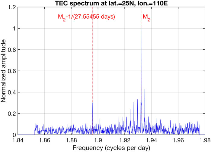
Figure 1 shows the selected frequency segment of the TEC spectrum in Southern China.

Figure 1

Figure 1. Selected frequency segment of the TEC spectrum in Southern China containing the lunar tide ${\text{M}}_2$ and its modulation peaks. The modulation peak of ${\text{M}}_2$ due to the anomalistic month occurs at the frequency of ${\text{M}}_2$ minus 1/(27.55455 days). The vertical red dashed line on the left-hand-side indicates this frequency position. The peaks of the solar semidiurnal tide are excluded in the selected frequency segment.

The modulation peaks of the solar semidiurnal tide (at a frequency of two cycles per day (cpd)) are mainly excluded in the selected frequency segment since the present article likes to investigate the Moon influences without influences by the solar semidiurnal tide ${\text{S}}_2$. However, it is likely that a small part of the noise on the right-hand-side of Figure 1 is due to modulations of ${\text{S}}_2$. Anyway, the lunar tide ${\text{M}}_2$ and its modulations clearly dominate in Figure 1, and it can be said that the lunar tide ${\text{M}}_2$ in TEC and its modulations have been isolated in the frequency domain.

For the further data analysis, the selected spectrum segment is transfered back to the time domain (by means of inverse FFT) yielding a time series $\mathrm{\Delta }$TEC. The modulations of the ${\text{M}}_2$ variations are investigated by means of filtering of the $\mathrm{\Delta }$TEC series with a digital non-recursive, finite impulse response bandpass filter. Zero-phase filtering is realized by processing the time series in forward and reverse directions. The filter has a Hamming window. The number of filter coefficients corresponds to a time window of three times the central period, so that the bandpass filter has a fast response time to temporal changes in the data series. The bandpass for the ${\text{M}}_2$ semidiurnal variation is open for all frequencies of the selected segment in Figure 1, and the bandpass cut-off frequencies are at the frequency of ${\text{M}}_2\pm 10\%$. Further details of the bandpass filtering are provided by Studer et al. (2012). Generally, the selected bandpass has a time resolution of about 1.5 days. The bandpass of the filter is rather broad but the $\mathrm{\Delta }$TEC was already limited to a narrow frequency region (without ${\text{S}}_2$) in the frequency domain. The envelope of the ${\text{M}}_2$ amplitude of the filtered $\mathrm{\Delta }$TEC series was calculated with a high time resolution as described by Studer et al. (2012). The envelope of the ${\text{M}}_2$ amplitude is mainly modulated by periods of the solar cycle, the annual cycle (and its harmonics), and the anomalistic month as a FFT spectral analysis of the envelope amplitude time series shows. The spectral analysis is performed in the same manner as described above.

The influence of the Moon orbit phase on ${\text{M}}_2$ in TEC can be studied by two methods. For the single grid point in Southern China, the filtered $\mathrm{\Delta }$TEC series is sorted and binned with respect to the Moon orbit phase from day 0 (Moon at perigee) to day 27.55455 (Moon at perigee again). Day 13.7773 stands for Moon at apogee. As reference point, the Moon perigee transit of 19 March 2011, 19:09 Greenwich Mean Time (GMT) was taken. The other (approximated) dates of perigee transits from 1998 to 2024 are given by assuming a mean anomalistic month of 27.55455 days for the return of the Moon perigee transit. Please note that the length of the anomalistic month can vary by several days due to gravitational perturbations of the Sun and Earth on the Moon’s eccentric orbit. The selected true perigee date (19 March 2011, 19:09 GMT) is optimal for the fit of a monochromatic wave with the period of the mean anomalistic month to the true (unevenly spaced) perigee dates from 2001 to 2024. The true perigee dates are listed by Fred Espenak at http://astropixels.com/ephemeris/moon/moonperap2001.html. The absolute value of the mean bias of the approximated, evenly spaced perigee datetimes with respect to the true perigee datetimes is less than 0.01 days. For the further data analysis, it is much easier to work with the series of the evenly spaced perigee datetimes.

The second method is to analyse the amplitude and phase of the FFT spectrum (of the filtered envelope series) at the period of the anomalistic month. This analysis can be easily performed for each grid point worldwide, so that one can derive world maps of the average amplitude and phase of the modulation effect of the anomalistic month. The Moon orbit phase of the FFT spectrum is derived from the phase difference between the FFT component and the phase of a cosine wave with maxima at the approximated perigee transits. Thus, Moon orbit phase 0° means that the maximum of the ${\text{M}}_2$ envelope appears at perigee. Phase 180° means that the maximum of the ${\text{M}}_2$ envelope is at apogee. Theory predicts that the ${\text{M}}_2$ variations in TEC are maximal a few days after perigee transit (3.0 days after perigee corresponds to a Moon orbit phase of 39.2°).

3 Results

The first result was already shown in Figure 1 of the previous section. Exactly at a frequency difference of 1/(27.55455 days) away from the ${\text{M}}_2$ frequency appears a significant modulation peak due to the anomalistic month which is the time from one perigee transit of the Moon to the next.

A 27 days-variation of TEC also can be due to the solar rotation period which varies from 25.67 days at the Sun’s equator to 33.40 days at 75$°$ latitude of the Sun. However, it is very unlikely that the variable solar rotation period is able to generate a single spectral peak exactly at the frequency position of the anomalistic month. Over the long time interval from 1998 to 2024, the Sun’s activity regions rotate in different latitude belts with different velocities so that a broad spectrum of line peaks due to the differential solar rotation can be expected from 26 to 29 days or so. Another reason is that the periods of the lunar variations are different from 24 h/n with n = 1, 2, 3, … Thus, the 27 days-solar acitivity variations are not in resonance with the lunar variations because the time points of the lunar maxima are drifting in solar time. Indeed, the modulation by the solar rotation period can be best seen in case of the solar diurnal ${\text{S}}_1$ variation of the TEC spectrum.

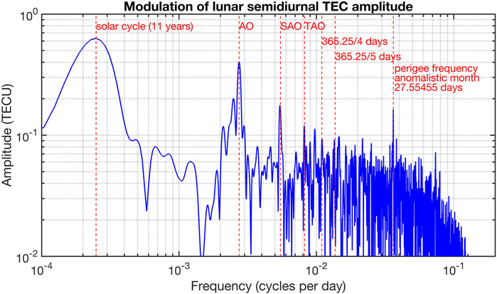
For the same grid point in Southern China (25$°$N latitude and 110$°$E longitude), the FFT spectrum of the $\mathrm{\Delta }$TEC envelope series of ${\text{M}}_2$ is calculated. Figure 2 shows the amplitude spectrum of the modulations of ${\text{M}}_2$ in TEC (without the effects of the solar semidiurnal tide ${\text{S}}_2$).

Figure 2

Figure 2. Amplitudes of modulations in ${\text{M}}_2$ in TEC as function of frequency in Southern China (25$°$N latitude and 110$°$E longitude). A modulation peak of ${\text{M}}_2$ due to the anomalistic month occurs at the frequency 1/(27.55455 days) indicated by the vertical red dashed line at the right-hand-side. The other vertical red dashed lines indicate the frequency positions of the solar cycle, the annual oscillation (AO) and its harmonics.

A modulation peak of ${\text{M}}_2$ due to the anomalistic month occurs at the frequency 1/(27.55455 days) indicated by the vertical red dashed line at the right-hand-side of Figure 2. In addition there are modulation peaks of ${\text{M}}_2$ related to the solar cycle, the annual oscillation (AO) and its harmonics. A possible modulation of ${\text{M}}_2$ by the quasi-biennial oscillation in stratospheric wind is less than 0.1 TECU.

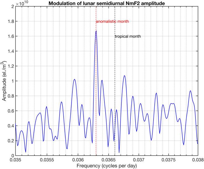
For verification of the modulation of ${\text{M}}_2$ in the ionosphere by the anomalistic month, the long-term series of NmF2 observed by the ionosonde at Okinawa is analysed in the same manner as the GNSS TEC data. Figure 3 shows the amplitude spectrum of the modulations of ${\text{M}}_2$ in NmF2 close to the period of the anomalistic month. It is obvious that exactly at the period of the anomalistic month a spectral peak occurs. There is no spectral peak at the period of the tropical month (27.32 days). Searching in the GNSS TEC spectra at other places worldwide, I did not find a convincing example where a significant spectral peak occurs at the period of the tropical month. The modulation peak at the anomalistic month of the ionosonde data at Okinawa is not so strong as in case of the GNSS TEC data in Southern China. This may indicate that the modulation effect of the anomalistic month is stronger in TEC than in NmF2. Another reason could be that the noise is larger for the ionosonde observations than for GNSS TEC. In addition, Okinawa (26.7 N) is a bit further northward of the EIA than the selected grid point in Southern China (25 N). Due to the strong meridional gradient in ionization at the EIA and the equatorial plasma fountain (Hargreaves, 1992), the EIA region is most sensitive to modulations by the Moon.

Figure 3

Figure 3. Amplitudes of modulations in ${\text{M}}_2$ in NmF2 as function of frequency observed by the ionosonde in Okinawa (26.7$°$N latitude and 128.1$°$E longitude). A modulation peak of ${\text{M}}_2$ due to the anomalistic month occurs at the frequency 1/(27.55455 days) indicated by the vertical red dashed line. The vertical black dashed line on the right-hand-side indicates the frequency position of the tropical month (27.32 days) where no spectral peak occurs.

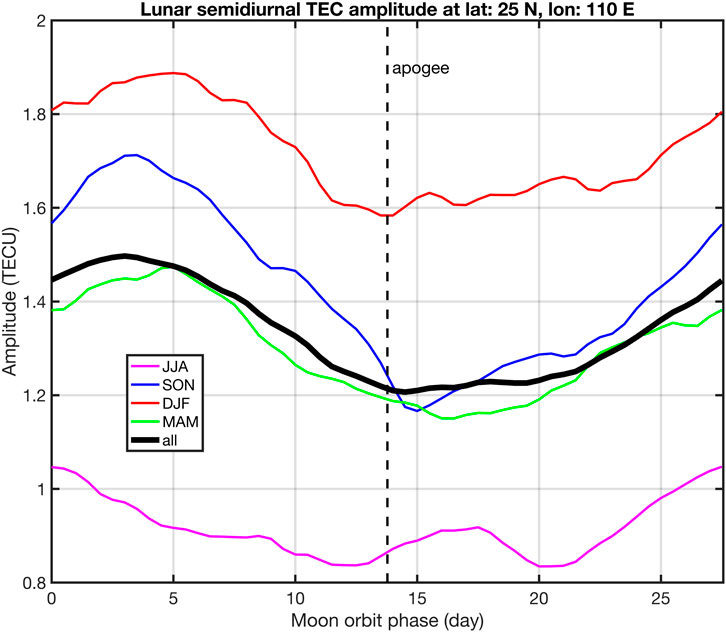
If we go back to the $\mathrm{\Delta }$TEC series in Southern China and sort and bin the values with respect to the Moon orbit phase, we get Figure 4. Day 0 of the Moon orbit phase means that the Moon is at perigee. At day 27.55455 the Moon is at perigee again. Day 13.7773 stands for the Moon at apogee as indicated by the vertical black dashed line in Figure 4.

Figure 4

Figure 4. Amplitude of ${\text{M}}_2$ in TEC as function of the Moon orbit phase (Southern China: 25$°$N latitude and 110$°$E longitude). The amplitude is maximal a few days after perigee transit of the Moon. The thick black curve is the result when the $\mathrm{\Delta }$TEC values of all seasons have been sorted and averaged.

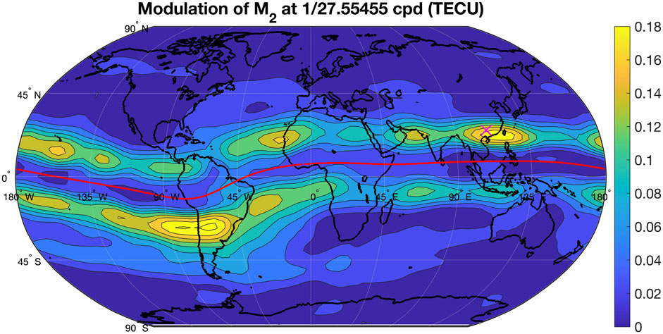
As described at the end of Section 2.3, global maps of the amplitude and phase of the modulation of ${\text{M}}_2$ in TEC by the anomalistic month can be retrieved. Figure 5 shows the result for the amplitude of the modulation peak of ${\text{M}}_2$ at the frequency 1/(27.55455 days). It is obvious that the modulation of ${\text{M}}_2$ by the anomalistic month is strongest in the EIA region in both hemispheres. There is also a longitudinal variability with amplitude maxima of up to 0.18 TECU in South America and Southern China. Generally, the amplitude distribution is a bit similar to the amplitude distribution of the ${\text{M}}_2$ amplitude which was shown by Hocke et al. (2025).

Figure 5

Figure 5. Amplitude of the modulation of ${\text{M}}_2$ in TEC by the anomalistic month (derived from the FFT spectrum of the $\mathrm{\Delta }$TEC envelope of ${\text{M}}_2$). The geomagnetic equator is indicated by the red line. The red cross denotes the location in Southern China (25$°$N, 110$°$E) which was analysed in Figures 1, 2, 4.

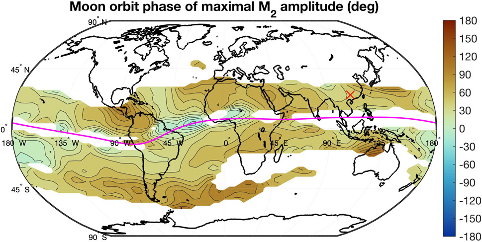
The calculation and definition of the Moon orbit phase were described at the end of Section 2.3. Moon orbit phase 0° means that the maximum of the ${\text{M}}_2$ envelope appears at perigee transit of the Moon. Phase 180° means that the maximum of the ${\text{M}}_2$ envelope is at apogee. Figure 6 shows the global map of the Moon orbit phase. Figure 6 only shows the values in the regions where the amplitude modulation of ${\text{M}}_2$ is greater than 0.03 TECU. The red cross denotes the location in Southern China (25$°$N, 110$°$E) where the Moon orbit phase has a value of 42.2°. This phase value means that the ${\text{M}}_2$ maximum in TEC is delayed by 3.2 days with respect to the perigee transit. This delay is in agreement with Figure 4 which is derived by a different method (composite of ${\text{M}}_2$ amplitudes with respect to the Moon orbit phase). If the Moon orbit phase of the maximum of ${\text{M}}_2$ is averaged for the regions where the modulation amplitude of ${\text{M}}_2$ is greater than 0.05 TECU, we get a mean value of 3.4 days delay (44.7°. The mean Moon orbit phase is 39.2°(3.0 days delay of ${\text{M}}_2$ maximum with respect to the perigee transit), if the average is taken for regions where the modulation amplitude is greater than 0.1 TECU. I would favour the mean phase value of the 0.1 TECU threshhold since the signal to noise ratio of the modulation peak of ${\text{M}}_2$ is better for a high threshhold value. It makes no sense to evaluate the Moon orbit phase at high latitudes where the signal of ${\text{M}}_2$ in TEC and its modulation by the anomalistic month are very weak and hidden by noise.

Figure 6

Figure 6. Moon orbit phase of the maximum of the ${\text{M}}_2$ amplitude in TEC (derived from the FFT spectrum of the $\mathrm{\Delta }$TEC envelope of ${\text{M}}_2$ at the period of the anomalistic month). Moon orbit phase 0$°$ means that the maximum of the ${\text{M}}_2$ envelope appears at perigee transit of the Moon. Phase 180$°$ means that the maximum of the ${\text{M}}_2$ envelope is at apogee. The geomagnetic equator is indicated by the red line. The red cross denotes the location in Southern China (25$°$N, 110$°$E) which was analysed in Figures 1, 2, 4. The Moon orbit phase at the red cross is 42.2°which means a delay of the ${\text{M}}_2$ maximum in TEC of 3.2 days with respect to the perigee transit. The figure only shows the Moon orbit phase for regions where the modulation of ${\text{M}}_2$ is greater than 0.03 TECU.

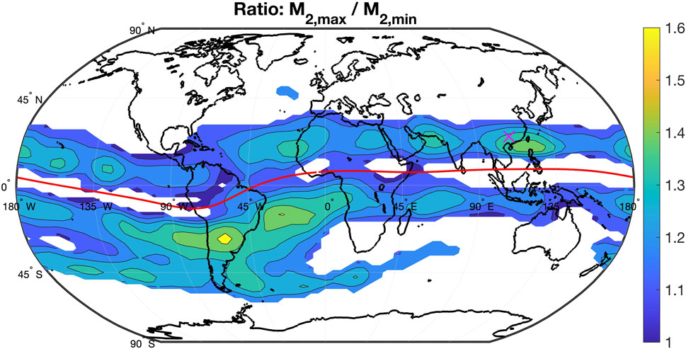
Finally, Figure 7 shows the ratio of the maximum of the ${\text{M}}_2$ amplitude in TEC and the minimum of the ${\text{M}}_2$ amplitude in TEC where by the maximum and minimum are caused by the variable Earth-Moon distance. The mean ratio is 1.25 for regions where the modulation of ${\text{M}}_2$ is greater than 0.1 TECU.

Figure 7

Figure 7. Ratio of the maximum of ${\text{M}}_2$ amplitude in TEC and the minimum of ${\text{M}}_2$ amplitude in TEC. Maximum and minimum are caused by the modulation of ${\text{M}}_2$ by the anomalistic month. The geomagnetic equator is indicated by the red line. The red cross denotes the location in Southern China (25$°$N, 110$°$E) which was analysed in Figures 1, 2, 4. The mean ratio is 1.25 for regions where the modulation of ${\text{M}}_2$ is greater than 0.1 TECU. The figure only shows the ratio values for regions where the modulation of ${\text{M}}_2$ is greater than 0.03 TECU.

4 Discussion

The analysis of the modulations of the ${\text{M}}_2$ amplitude (Figure 2) showed that the quasi-biennial oscillation in middle atmospheric wind only plays a minor role for the upward propagation of the lunar tide. The lunar tide in TEC is mainly modulated by the solar cycle, annual oscillation and its harmonics and the variable Earth-Moon distance. There are several factors which may explain the modulations, e.g., solar and seasonal cycles in ionization, seasonal cycle in atmospheric wind fields.

The most important result of the present study is that the ${\text{M}}_2$ amplitude is modulated by the anomalistic month. Figure 2 shows a significant spectral peak at the period of the anomalistic month which is comparable to the modulation of ${\text{M}}_2$ variation by the semiannual oscillation (SAO). The modulation of ${\text{M}}_2$ by the anomalistic month is due to the eccentric orbit of the Moon which causes larger lunar tides when the Moon is near to the perigee (closest distance of Moon and Earth).

The amplification of lunar tides during the perigee transit of the Moon is well known in oceanography where perigean spring tides have maximal tidal changes in sea level height since the Moon phase is Full Moon or New Moon (constructive interference of solar and lunar gravitational and centrifugal forcing of ${\text{M}}_2$) and the Moon is in the perigee of the elliptical Moon orbit (closest Earth-Moon distance with strongest gravitational forcing of ${\text{M}}_2$). In case of atmospheric tides the situation is a bit different since the solar atmospheric tides are not due to gravitational forcing of the Sun but due to thermal forcing by insolation of the atmosphere. In the present study, the long-term time series of GNSS observations allowed a separation of the lunar tide ${\text{M}}_2$ in TEC from the solar tide ${\text{S}}_2$ in TEC. Thus, the present study is focused on the eccentricity modulation of ${\text{M}}_2$ in TEC which might be called ionospheric perigean tide.

Equilibrium theory of tides predict that the amplitude of perigean tides are greater than the apogean tides as it follows. The tide constant [Gezeitenkonstante in Kertz (1989)] of the Moon is $G_L$:

$G_L=\frac{3}{4}\frac{\gamma M_L{R}_E^2}{r_L^3}(2)$

where $\gamma$ is the gravitational constant, $M_L$ is the mass of the Moon, $R_E$ is the Earth radius, and $r_L$ is the Earth-Moon distance. The equilibrium elevation $\bar{\zeta }$ of the ${\text{M}}_2$ tidal bulge (tidal change of sea level) is given by Kertz (1989)

$\bar{\zeta }=\frac{G_L}{g}\left(\cos 2\vartheta +\frac{1}{3}\right)(3)$

where $g$ is the gravity acceleration at the Earth’s surface and $\vartheta$ is the geographic latitude (if Moon is in the equatorial plane of the Earth).

The ratio $R$ of the equilibrium elevations at perigee $\overline{{\zeta }_p}$ and apogee $\overline{{\zeta }_a}$ is

$R=\frac{\overline{{\zeta }_p}}{\overline{{\zeta }_a}}=\frac{G_{L,p}}{G_{L,a}}=\frac{r_{L,a}^3}{r_{L,p}^3}=\frac{405400^3}{362600^3}=1.40(4)$

where an Earth-Moon distance of 405,400 km is taken for apogee and 362,600 km is taken for perigee. It can be assumed that the ratio of surface air pressure of ${\text{M}}_2$ at perigee and at apogee is similar to the ratio of equilibrium elevations. Indeed, Figure 7 shows that the mean ratio of ${\text{M}}_2$ maximum in TEC and ${\text{M}}_2$ minimum in TEC is 1.25 for regions where the modulation of ${\text{M}}_2$ is greater than 0.1 TECU. The value of 1.25 in the ionosphere is not so far away from the theoretical value of 1.40 at the ocean surface, since the lunar tide may experience amplitude-dependent dissipation processes. It is likely that the amplitude ratio slightly changes when the lunar tide propagates to the dynamo region and when the tide-induced electric field variations cause a ${\text{M}}_2$ variation in TEC at low magnetic latitudes.

The analysis also showed that the maximal ${\text{M}}_2$ amplitude in TEC was delayed by 3.0 days with respect to the time point of the perigee transit (Figures 4, 6). The value of 3.0 days was calculated for the regions where the ${\text{M}}_2$ modulation is greater than 0.1 TECU. It was already suggested that this delay is due to the travel time of the lunar tide from the surface to the ionosphere. According to theoretical studies and numerical simulations, tidal wave modes require several days for their travel from the surface to the lower ionosphere (about 100 km altitude) (Richmond, 1975; Vial et al., 1991; Aso, 1993; Walterscheid, 1997). The analytical formulas for the calculation of the vertical group velocities of various solar and lunar tidal wave modes (Richmond, 1975) have been used for the lunar tidal wave modes (2,2), (2,3) and (2,4) yielding travel times of 2.5 days, 2.2 days and 2.8 days for the distance from the surface to 105 km altitude. For calculation of these values, a constant temperature profile of 250 K was taken. The theoretical vertical group velocities of the lunar tidal wave modes (2,2), (2,3) and (2,4) are 42.2 km/day, 48.4 km/day and 37.6 km/day respectively. Theoretical delay times of the lunar tide (Richmond, 1975) fit quite well to the observed value of 3.0 days delay of the maximal ${\text{M}}_2$ amplitude in TEC with respect to the perigee transit. The fast response time of the surface air tide to the changing Earth-Moon distance is neglected here as well as the fast transfer time of the electric field variations from the E region to the F region where electrodynamic lifting of the plasma occurs.

The geographical distribution of the ${\text{M}}_2$ modulation in TEC (Figure 5) is related to the ${\text{M}}_2$ amplitude in TEC which was discussed in Hocke et al. (2025). This is expected since the modulation of the lunar tide is about 11% of the mean ${\text{M}}_2$ amplitude. The 11% modulation gives the observed value of 1.25 for the ratio of maximal ${\text{M}}_2$ and minimal ${\text{M}}_2$ in TEC which is induced by the eccentricity of the Moon orbit. The longitudinal variablity of the ${\text{M}}_2$ amplitude in TEC and its modulation may depend on variability in the vertical propagation conditions of the lunar tide, and longitudinal differences in the ionization and electrodynamic lifting process. It might be questionable in how far a non-migrating tide explanation can be applied for the lunar tide since the tidal excitation is not depending on insolation of variable tropospheric water and ozone distributions.

5 Conclusion

The worldwide network of GNSS receivers (International GNSS Service) monitors the total electron content (TEC) since 1998 and allows to study the influences of the Moon on the Earth’s ionosphere in detail. The long-term time series of TEC allows a separation of the lunar ${\text{M}}_2$ spectral line and its modulation peaks from the signal of the solar semidiurnal tide ${\text{S}}_2$ (Figure 1). It was shown that the ${\text{M}}_2$ amplitude in TEC is modulated by the period of the anomalistic month (27.55455 days). Ionosonde data at Okinawa supported this finding and showed a Moon orbit eccentricity modulation of ${\text{M}}_2$ in the long-term time series of ${\text{F}}_2$ peak electron density. Significant modulation of ${\text{M}}_2$ in the ionosphere by the tropical month (27.32 days) or the quasi-biennial oscillation were not found while the modulations of ${\text{M}}_2$ by the solar cycle, the annual oscillation and its harmonics are obvious.

The ${\text{M}}_2$ amplitude in TEC after perigee is by a factor of 1.25 larger than the ${\text{M}}_2$ amplitude in TEC after apogee while equilibrium theory of tides predicts a factor of 1.40 for the perigee-to-apogee ratio of the lunar tide in equilibrium elevation of the ocean surface. It is found that the maximal ${\text{M}}_2$ amplitude in TEC occurs about 3.0 days after the perigee transit of the Moon. The observed delay of 3.0 days indicates that the lunar tide may require 3 days for the travel from the lower atmosphere to the dynamo region. Analytical equations of tidal wave theory (Richmond, 1975) show that the lunar tidal wave modes (2,2), (2,3), (2,4) require travel times of 2.5 days, 2.2 days, and 2.8 days from 0 km to 105 km altitude, depending on their vertical group velocities (assuming a constant temperature profile of 250 K).

The observed lunar tide in TEC and its eccentricity modulation seem to be a valuable tool for the study of vertical propagation of the lunar tide from the surface to the ionospheric dynamo region. The lunar tide in TEC is interesting for model-observation intercomparisons since the lunar tide does not depend on insolation of highly variable tropospheric water and stratospheric ozone fields, so that the lunar tide might be a good indicator for the impact of temperature and wind profiles on the vertical propagation of tides. It is of interest for space weather and atmosphere-ionosphere coupling how fast tides can transfer energy and momentum from the lower atmosphere to the ionosphere.

Data availability statement

Publicly available datasets were analyzed in this study. This data can be found here: https://wdc.nict.go.jp/IONO/HP2009/ISDJ/manual_txt-E.html, https://cddis.nasa.gov/.

Author contributions

KH: Conceptualization, Formal Analysis, Investigation, Methodology, Software, Validation, Writing – original draft, Writing – review and editing.

Funding

The author(s) declare that financial support was received for the research and/or publication of this article. Open access funding was provided by the University of Bern and swissuniversities. Open access funding by University of Bern Giorgia.

Acknowledgments

I thank Yosuke Yamazaki for a discussion of some of the results. I thank the International GNSS Service (IGS) for providing TEC maps. The World Data Center for Ionosphere and Space Weather, Tokyo, National Institute of Information and Communications Technology is thanked for providing the long-term $foF2$ series at Okinawa and for operation of the ionosonde. Planetary Ephemeris Data Courtesy of Fred Espenak, www.Astropixels.com.

Conflict of interest

The author declares that the research was conducted in the absence of any commercial or financial relationships that could be construed as a potential conflict of interest.

Generative AI statement

The author(s) declare that no Gen AI was used in the creation of this manuscript.

Publisher’s note

All claims expressed in this article are solely those of the authors and do not necessarily represent those of their affiliated organizations, or those of the publisher, the editors and the reviewers. Any product that may be evaluated in this article, or claim that may be made by its manufacturer, is not guaranteed or endorsed by the publisher.

References

Aso, T. (1993). Time-dependent numerical modelling of tides in the middle atmosphere. J. geomagnetism Geoelectr. 45, 41–63. doi:10.5636/jgg.45.41

CrossRef Full Text | Google Scholar

Chuo, Y. J. (2012). Variations of ionospheric profile parameters during solar maximum and comparison with iri-2007 over chung-li, taiwan. Ann. Geophys. 30, 1249–1257. doi:10.5194/angeo-30-1249-2012

CrossRef Full Text | Google Scholar

Davies, K. (1990). Ionospheric radio. London: Peter Peregrinus.

Google Scholar

Forbes, J. M., and Zhang, X. (2012). Lunar tide amplification during the january 2009 stratosphere warming event: observations and theory. J. Geophys. Res. Space Phys. 117. doi:10.1029/2012JA017963

CrossRef Full Text | Google Scholar

Hagan, M., Forbes, J., and Richmond, A. (2003). “Atmospheric tides,” in Encyclopedia of atmospheric sciences. Editor J. R. Holton (Oxford: Academic Press), 159–165. doi:10.1016/B0-12-227090-8/00409-7

CrossRef Full Text | Google Scholar

Hargreaves, J. K. (1992). “The solar-terrestrial environment: an introduction to geospace - the science of the terrestrial upper atmosphere, ionosphere, and magnetosphere,” in Cambridge atmospheric and space science series. Cambridge University Press. doi:10.1017/CBO9780511628924

CrossRef Full Text | Google Scholar

Hernández-Pajares, M., Juan, J. M., Sanz, J., Orus, R., Garcia-Rigo, A., Feltens, J., et al. (2009). The igs vtec maps: a reliable source of ionospheric information since 1998. J. Geodesy 83, 263–275. doi:10.1007/s00190-008-0266-1

CrossRef Full Text | Google Scholar

Hocke, K., Pedatella, N. M., and Yamazaki, Y. (2025). Nonlinear interaction of the lunar tide m2 and the diurnal variation of electron density in the ionosphere. J. Geophys. Res. Space Phys. 130, e2024JA033482. doi:10.1029/2024ja033482

CrossRef Full Text | Google Scholar

Hocke, K., Wang, W., Cahyadi, M. N., and Ma, G. (2024). Quasi-diurnal lunar tide o1 in ionospheric total electron content at solar minimum. J. Geophys. Res. Space Phys. 129, e2024JA032834. doi:10.1029/2024ja032834

CrossRef Full Text | Google Scholar

Kertz, W. (1989). Einführung in die Geophysik 1. B.I. Hochschultaschenbücher Band. 275.

Google Scholar

Kvale, E. P. (2006). The origin of neap-spring tidal cycles. Mar. Geol. 235, 5–18. doi:10.1016/j.margeo.2006.10.001

CrossRef Full Text | Google Scholar

Lin, J. T., Lin, C. H., Lin, C. Y., Pedatella, N. M., Rajesh, P. K., Matsuo, T., et al. (2019). Revisiting the modulations of ionospheric solar and lunar migrating tides during the 2009 stratospheric sudden warming by using global ionosphere specification. Space weather. 17, 767–777. doi:10.1029/2019SW002184

CrossRef Full Text | Google Scholar

Lindzen, R. S., and Chapman, S. (1969). Atmospheric tides. Space Sci. Rev. 10, 3–188. doi:10.1007/BF00171584

CrossRef Full Text | Google Scholar

Pedatella, N. M., and Liu, H. (2013). The influence of atmospheric tide and planetary wave variability during sudden stratosphere warmings on the low latitude ionosphere. J. Geophys. Res. Space Phys. 118, 5333–5347. doi:10.1002/jgra.50492

CrossRef Full Text | Google Scholar

Pedatella, N. M., Liu, H.-L., Sassi, F., Lei, J., Chau, J. L., and Zhang, X. (2014). Ionosphere variability during the 2009 ssw: influence of the lunar semidiurnal tide and mechanisms producing electron density variability. J. Geophys. Res. Space Phys. 119, 3828–3843. doi:10.1002/2014JA019849

CrossRef Full Text | Google Scholar

Pertsev, N., Dalin, P., and Perminov, V. (2023). The 27.3-day oscillation in the lunar tidal theory and in atmospheric data. J. Atmos. Solar-Terrestrial Phys. 242, 106002. doi:10.1016/j.jastp.2022.106002

CrossRef Full Text | Google Scholar

Richmond, A. D. (1975). Energy relations of atmospheric tides and their significance to approximate methods of solution for tides with dissipative forces. J. Atmos. Sci. 32, 980–987. doi:10.1175/1520-0469(1975)032<0980:eroata>2.0.co;2

CrossRef Full Text | Google Scholar

Schindelegger, M., Sakazaki, T., and Green, M. (2023). “Chapter 16 - atmospheric tides—an earth system signal,” in A journey through tides. Editors M. Green, and J. C. Duarte (Elsevier), 389–416. doi:10.1016/B978-0-323-90851-1.00007-8

CrossRef Full Text | Google Scholar

Studer, S., Hocke, K., and Kämpfer, N. (2012). Intraseasonal oscillations of stratospheric ozone above Switzerland. J. Atmos. Solar-Terrestrial Phys. 74, 189–198. doi:10.1016/j.jastp.2011.10.020

CrossRef Full Text | Google Scholar

Talari, P., and Panda, S. K. (2019). Occurrences of counter electrojets and possible ionospheric tec variations round new moon and full moon days across the low latitude indian region. J. Appl. Geodesy 13, 245–255. doi:10.1515/jag-2019-0014

CrossRef Full Text | Google Scholar

Vial, F., Forbes, J. M., and Miyahara, S. (1991). Some transient aspects of tidal propagation. J. Geophys. Res. Space Phys. 96, 1215–1224. doi:10.1029/90JA02181

CrossRef Full Text | Google Scholar

Walterscheid, R. L. (1997). Simple models of tidal transience: the steady state signal. J. Geophys. Res. Atmos. 102, 25807–25815. doi:10.1029/97JD02079

CrossRef Full Text | Google Scholar

Wu, T.-Y., Liu, J.-Y., Lin, C.-Y., and Chang, L. C. (2020). Response of ionospheric equatorial ionization crests to lunar phase. Geophys. Res. Lett. 47, e2019GL086862. doi:10.1029/2019gl086862

CrossRef Full Text | Google Scholar

Yamazaki, Y., and Richmond, A. D. (2013). A theory of ionospheric response to upward-propagating tides: electrodynamic effects and tidal mixing effects. J. Geophys. Res. Space Phys. 118, 5891–5905. doi:10.1002/jgra.50487

CrossRef Full Text | Google Scholar

Yamazaki, Y., Richmond, A. D., and Yumoto, K. (2012). Stratospheric warmings and the geomagnetic lunar tide: 1958-2007. J. Geophys. Res. Space Phys. 117. doi:10.1029/2012JA017514

CrossRef Full Text | Google Scholar

Yamazaki, Y., Stolle, C., Matzka, J., Siddiqui, T. A., Luehr, H., and Alken, P. (2017). Longitudinal variation of the lunar tide in the equatorial electrojet. J. Geophys. Res. Space Phys. 122, 12,445–512. doi:10.1002/2017JA024601

CrossRef Full Text | Google Scholar

Zhang, J. T., and Forbes, J. M. (2013). Lunar tidal winds between 80 and 110 km from UARS/HRDI wind measurements. J. Geophys. Res. Space Phys. 118, 5296–5304. doi:10.1002/jgra.50420

CrossRef Full Text | Google Scholar

Zhang, J. T., Forbes, J. M., Zhang, C. H., Doornbos, E., and Bruinsma, S. L. (2014). Lunar tide contribution to thermosphere weather. Space weather. 12, 538–551. doi:10.1002/2014SW001079

CrossRef Full Text | Google Scholar