 Scott D. Chambers1*
 Susanne Preunkert2Rolf Weller3
 Sang-Bum Hong4
 Ruhi S. Humphries5,6
 Laura Tositti7
 Hélène Angot8Michel Legrand2
 Alastair G. Williams1Alan D. Griffiths1Jagoda Crawford1Jack Simmons6
 Taejin J. Choi4Paul B. Krummel5Suzie Molloy5Zoë Loh5Ian Galbally5
 Stephen Wilson6
 Olivier Magand2
 Francesca Sprovieri9Nicola Pirrone9
 Aurélien Dommergue2
- 1Environmental Research, ANSTO, Sydney, NSW, Australia
- 2CNRS, IRD, IGE, University Grenoble Alpes, Grenoble, France
- 3Alfred Wegener Institute for Polar and Marine Research, Bremerhaven, Germany
- 4Korea Polar Research Institute, Incheon, South Korea
- 5Climate Science Centre, CSIRO Oceans and Atmosphere, Aspendale, VIC, Australia
- 6Centre for Atmospheric Chemistry, University of Wollongong, Wollongong, NSW, Australia
- 7Environmental Chemistry and Radioactivity Lab, University of Bologna, Bologna, Italy
- 8Institute for Data, Systems and Society, Massachusetts Institute of Technology, Cambridge, MA, United States
- 9CNR-Institute of Atmospheric Pollution Research, Monterotondo, Italy
We discuss remote terrestrial influences on boundary layer air over the Southern Ocean and Antarctica, and the mechanisms by which they arise, using atmospheric radon observations as a proxy. Our primary motivation was to enhance the scientific community’s ability to understand and quantify the potential effects of pollution, nutrient or pollen transport from distant land masses to these remote, sparsely instrumented regions. Seasonal radon characteristics are discussed at 6 stations (Macquarie Island, King Sejong, Neumayer, Dumont d’Urville, Jang Bogo and Dome Concordia) using 1–4 years of continuous observations. Context is provided for differences observed between these sites by Southern Ocean radon transects between 45 and 67°S made by the Research Vessel Investigator. Synoptic transport of continental air within the marine boundary layer (MBL) dominated radon seasonal cycles in the mid-Southern Ocean site (Macquarie Island). MBL synoptic transport, tropospheric injection, and Antarctic outflow all contributed to the seasonal cycle at the sub-Antarctic site (King Sejong). Tropospheric subsidence and injection events delivered terrestrially influenced air to the Southern Ocean MBL in the vicinity of the circumpolar trough (or “Polar Front”). Katabatic outflow events from Antarctica were observed to modify trace gas and aerosol characteristics of the MBL 100–200 km off the coast. Radon seasonal cycles at coastal Antarctic sites were dominated by a combination of local radon sources in summer and subsidence of terrestrially influenced tropospheric air, whereas those on the Antarctic Plateau were primarily controlled by tropospheric subsidence. Separate characterization of long-term marine and katabatic flow air masses at Dumont d’Urville revealed monthly mean differences in summer of up to 5 ppbv in ozone and 0.3 ng m-3 in gaseous elemental mercury. These differences were largely attributed to chemical processes on the Antarctic Plateau. A comparison of our observations with some Antarctic radon simulations by global climate models over the past two decades indicated that: (i) some models overestimate synoptic transport to Antarctica in the MBL, (ii) the seasonality of the Antarctic ice sheet needs to be better represented in models, (iii) coastal Antarctic radon sources need to be taken into account, and (iv) the underestimation of radon in subsiding tropospheric air needs to be investigated.
Introduction
The Southern Hemisphere is currently home to only around 10% of the global population, and non-Antarctic land masses cover less than 14% of its surface. These factors, combined with the vast extent of the Southern Ocean and efficient wet deposition removal within the circumpolar trough, have so far ensured that Antarctica has remained one of the most pristine places on earth. However, the presence of artificial radioactivity following weapons testing (Koide et al., 1979), the Antarctic ozone hole (Solomon, 1999), and ice core trace gas analyses (Etheridge et al., 1996), constitute some of the irrefutable evidence that anthropogenic influences have impacted this region for many decades. Still, the relatively pristine Antarctic atmosphere provides a rare opportunity to explore an approximation of pre-industrial conditions, and its seasonal meteorological extremes also provide unique opportunities to explore a range of surface and atmospheric chemical processes (Crawford et al., 2001; Davis et al., 2001; Eisele et al., 2008; Jones et al., 2008; Preunkert et al., 2008; Slusher et al., 2010; Angot et al., 2016c; Legrand et al., 2016).
The crucial role Antarctica plays in global atmospheric and oceanic circulation is well established, as is the importance of the expansive Southern Ocean to global climate, atmospheric composition, and marine life everywhere (Bromwich et al., 1993; Nicol et al., 2000; Gille, 2002; Manno et al., 2007; Sandrini et al., 2007; Stavert et al., 2018). Recent investigations have also shown that Antarctica’s ice sheets, which provide a valuable window through which to view the past (Jouzel et al., 2007; Brook and Buizert, 2018), and hold around 70% of the world’s fresh water (Fox et al., 1994), are particularly susceptible to the influences of climate change (Turner et al., 2006; DeConto and Pollard, 2016; Rintoul et al., 2018). Consequently, methods to improve the understanding of transport pathways of terrestrially influenced air masses (potentially containing pollutants, nutrients, pollen, etc.) to these remote and changing regions is of multidisciplinary interest (e.g., Jickells et al., 2005).
While some pollutants and trace atmospheric constituents found in Antarctic and sub-Antarctic regions are generated locally (via shipping, research bases, wildlife, volcanic activity and photochemical processes; Jones et al., 2008; Shirsat and Graf, 2009; Graf et al., 2010; Bargagli, 2016), the balance of these species are attributable to remote sources, primarily of terrestrial origin. Remotely sourced trace gasses and aerosols travel to Antarctica and the remote Southern Ocean by one of two pathways (Polian et al., 1986; Krinner et al., 2010; Chambers et al., 2014, 2017): directly, as a result of synoptic transport within the marine boundary layer (MBL), or indirectly, as a result of subsiding or intruding tropospheric air that has experienced recent continental influences (e.g., through deep convection or frontal uplift; e.g., Belikov et al., 2013).
While some terrestrial emissions travel great distances to reach Antarctica (e.g., from the Northern Hemisphere; Mahowald et al., 1999; Li et al., 2008), the majority of such material is typically of Southern Hemispheric origin (e.g., Albani et al., 2012), traveling over timescales and pathways that can be elucidated by measurements of the radioactive terrestrial tracer Radon-222 (radon). Having a short half-life (3.82 days) and an almost exclusively terrestrial source function, this noble gas provides an unambiguous means of characterizing the degree of recent terrestrial influence on air masses. In recent decades improvements in radon measurement technology have enabled routine detection down to concentrations of 5 – 40 mBq m-3 (e.g., Whittlestone and Zahorowski, 1998; Levin et al., 2002; Chambers et al., 2014, 2016; Williams and Chambers, 2016; Chambers and Sheppard, 2017). With detectors of this kind it is possible to track the movement of terrestrially influenced air masses over oceans (or in the troposphere) for up to 3 weeks.
Over the past four decades there has been a gradually expanding international network of continuous atmospheric radon monitors throughout Antarctica and the Southern Ocean. The resulting datasets have been highly valuable for “baseline” (hemispheric background) studies (e.g., Brunke et al., 2004; Zahorowski et al., 2013; Chambers et al., 2016), transport and mixing studies (Tositti et al., 2002; Pereira et al., 2006; Weller et al., 2014; Chambers et al., 2014, 2017), and as a tool for the evaluation of numerical model performance (e.g., Dentener et al., 1999; Law et al., 2010; van Noije et al., 2014; Locatelli et al., 2015).
Furthermore, an experimental meteorological technique was recently developed by Chambers et al. (2017) by which Antarctic air masses could be broadly separated into oceanic, coastal or katabatic fetch categories. Since many Antarctic research bases are in coastal locations, and free-tropospheric, Antarctic Plateau, coastal, and marine air masses have quite distinct properties, the ability to interpret atmospheric observations relies heavily on an ability to reliably identify air mass fetch. While simulated back trajectories have often been employed in this regard (e.g., Markle et al., 2012; Angot et al., 2016b), a dearth of supporting observations, the complex topography, and highly stable atmospheric conditions, pose significant sources of simulation error in this region. Combining high quality radon observations (a proxy for terrestrial influence) with experimental fetch analyses techniques, stands to add yet another dimension to interpretations of Antarctic atmospheric observations.
The main aims of this study are: to summarize a collection of long-term radon observations in Antarctica and the remote southern ocean (some of which are still ongoing), to introduce Southern Ocean radon observations from the mobile platform RV Investigator, and to demonstrate the insight provided by such observations to transport processes in these remote regions (with particular emphasis on the circumpolar trough and Antarctic coast). As brief examples of the potential value to be added to Antarctic atmospheric research by the datasets and techniques described in this study, we also show some selected results from investigations of aerosols (cloud condensation nuclei), carbon dioxide, ozone and gaseous elemental mercury (GEM, Hg0). More detailed investigation of these species is beyond the scope of this study and will be the subject of future investigations.
Materials and Methods
Radon: A Proxy for Recent Terrestrial Influence on an Air Mass
Radon-222 (radon) is a gaseous decay product of Uranium-238. Its immediate parent, Radium-226, is ubiquitous in soils and rocks. Radon is a noble gas, poorly soluble, and radioactive (t0.5 = 3.82 days), so it does not accumulate in the atmosphere on greater than synoptic timescales. Its average source function from unfrozen terrestrial surfaces is relatively well constrained (0.7 – 1.2 atoms cm-2 s-1, Zhang et al., 2011; 1.0–1.25 atoms cm-2 s-1, Griffiths et al., 2010; 0.4–1.0 atoms cm-2 s-1, Karstens et al., 2015), and 2–3 orders of magnitude greater than that from the open ocean (Schery and Huang, 2004). Furthermore, on regional scales radon’s terrestrial source function is not significantly affected by human activity. This combination of physical characteristics enables air masses that have been in contact with terrestrial surfaces to be tracked over the ocean, or within the troposphere, for 2–3 weeks. Consequently, radon observations constitute a convenient, economical, and unambiguous indicator of recent terrestrial influence on air masses. Since the majority of anthropogenic gaseous and aerosol pollutants are also of terrestrial origin, high-quality radon observations serve as a proxy for the ‘pollution potential’ of air masses in remote regions.
The radon concentration of air masses that have been in long-term equilibrium with the Southern Ocean is typically 30–50 mBq m-3 (e.g., Zahorowski et al., 2013; Chambers et al., 2016; Crawford et al., 2018). Consequently, key requirements of radon detectors deployed in such remote locations are: a detection limit of ≤50 mBq m-3, stable absolute calibrations, and low maintenance.
Radon campaigns of varying duration and temporal resolution were conducted in and around Antarctica between 1960 and 1990 (see reviews by Polian et al., 1986; Ui et al., 1998; Chambers et al., 2014). In recent decades, however, the availability of continuous, long-term, high-quality radon observations at Southern Ocean and Antarctic stations has been slowly improving (e.g., Tositti et al., 2002; Pereira et al., 2004; Brunke et al., 2004; Zahorowski et al., 2013; Chambers et al., 2014, 2017; Weller et al., 2014). Detection methods have included electrostatic deposition (Pereira and da Silva, 1989; Ui et al., 1998; Tositti et al., 2002), static single-filter detectors (Levin et al., 2002), and two-filter detectors (Chambers et al., 2014). Stations presently contributing to the Southern Ocean network of radon detectors include: Cape Grim (CG), Baring Head (BH), Cape Point (CP), Macquarie Island (MI), Jang Bogo (JBS), King Sejong (KSG), and Neumayer (NM) (Figure 1).
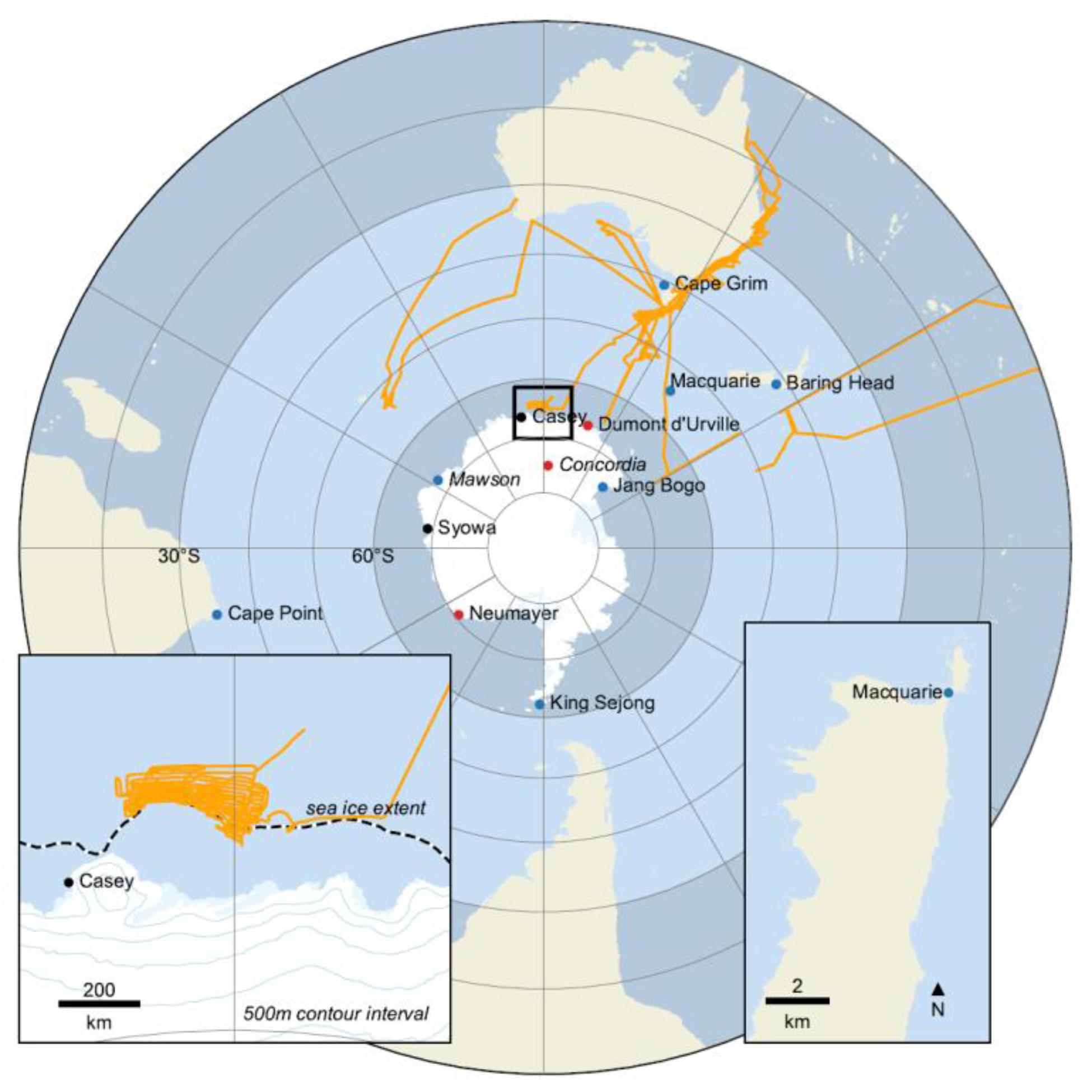
FIGURE 1. Southern Ocean radon detector network: two-filter detectors (blue), single-filter detectors (red). RV Investigator cruise track (January 2015 to June 2017) shown in orange. Inset 1 shows RV Investigator maneuvers for sea floor mapping (January–February 2017), and includes the February 2017 sea ice extent based on the 20% concentration contour from passive microwave satellite data (Peng et al., 2013; Meier et al., 2017). Ice sheet elevation contours are from ETOPO1 (Amante and Eakins, 2009). Inset 2 shows location of Macquarie Island monitoring station with coastline data from Natural Earth and, for the Macquarie Island inset, the Australian Antarctic Division (2005).
Sites and Equipment
This article summarizes radon and auxiliary observations (e.g., meteorology, trace gasses and aerosols) from four of the long-term ongoing monitoring stations in the Southern Ocean network (MI, KSG, NM, and JBS), as well as Dumont d’Urville (DDU), Dome Concordia (DC), and selected observations from the Research Vessel Investigator (Table 1). Brief mention is also made of previously published observations from Mawson Base (Chambers et al., 2014). All reported times are local station times. For RV Investigator and MI observations the standard Southern Hemisphere seasonal convention has been adopted. For the Antarctic bases “summer” refers to the period November through February, “winter” the period April through September; March and October are considered transitional months.
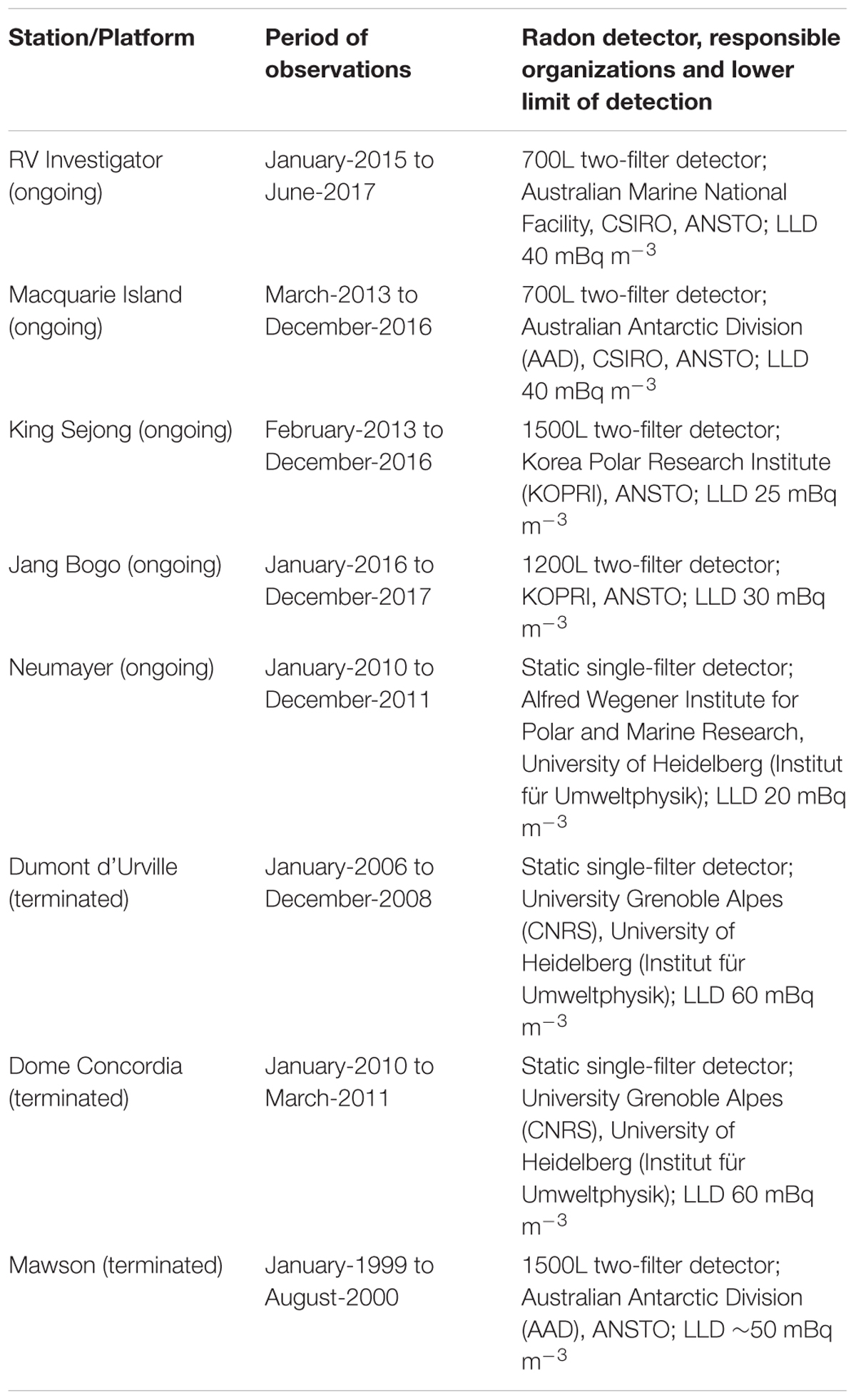
TABLE 1. Sites, detection method, time periods, and responsible organizations for observations discussed in this study.
The RV Investigator’s radon detector was installed in September 2014 in the Aerosol Sampling Laboratory at the bow of the vessel, immediately below the sampling mast on the foredeck. Sample air is drawn at 65–75 L min-1 from a goose-neck inlet at 15 m above the foredeck (around 20–22 m above sea level, a.s.l.) through 25 mm HDPE agricultural pipe. A coarse aerosol filter, dehumidifier and water trap are installed upstream of the detector, to protect the detector’s primary filter and internal components. Calibrations are performed on either a campaign or quasi-monthly basis by injecting radon from a PYLON Radon-222 source (20.62 ± 4% kBq 226Ra, delivering 2.598 Bq min-1 222Rn)1 for 6 h at a flow rate of ∼100 cc min-1, and the instrumental background is checked either on a campaign basis or every 3 months. Details of other atmospheric observations aboard the RV Investigator are given in Protat et al. (2016).
Macquarie Island is small (34 × 5 km), and is situated roughly midway between Australia and Antarctica (Figure 1). Radon and meteorological observations are made at the “Clean Air Laboratory” on an isthmus at the northern end of the island (∼54.5°S; Figure 1, inset 2). The MI radon detector was installed in March 2011, but technical problems delayed the start of the sampling program until March 2013. Sample air is drawn at ∼45 L m-1 from an inlet ∼5 m above ground level (a.g.l.) on a 10 m mast. The detector is calibrated monthly using a similar source to the RV Investigator (19.58 ± 4% kBq 226Ra) injecting for 6 h at a flow rate of ∼170 cc min-1. Instrumental background checks are performed quarterly by stopping the internal and external flow loop blowers for 24 h. Further information about MI observations can be found in Brechtel et al. (1998) and Stavert et al. (2018).
A similar protocol is followed for the two-filter detectors at KSG and JBS. For details the reader is referred to existing publications (Chambers et al., 2014, 2017). Further details about the regions surrounding KSG and JBS are given in Evangelista and Pereira (2002) and Tositti et al. (2002).
Radon observations at NM, DDU, and DC were all made using single-filter (“by progeny”) Heidelberg Radon Monitors (HRM, Levin et al., 2002). The current system providing 3-hourly radon observations at Neumayer Station has been in place since 1995. Specific details about the site as well as the setup and operation of the Neumayer HRM and other observations are provided in Weller et al. (2014). Specifically regarding the NM radon sampling inlet, ambient air is first sucked through 3 m of 200 mm electro-polished stainless steel at 8.8 m s-1, then through 2.8 m of 50 mm electro-polished stainless steel tube at 2 m s-1, and finally through ∼50 cm of 6 mm stainless steel tube at 21 m s-1.
At DDU the HRM was setup in laboratory “Labo 3” (e.g., Preunkert et al., 2012) in which other long-term atmospheric measurements such as ozone (Legrand et al., 2009, 2016), sulfur species (Preunkert et al., 2008), gaseous elemental mercury (GEM, 2012–2015; Angot et al., 2016c; Sprovieri et al., 2016), other aerosols and reactive gasses are also conducted. The radon measurement resolution was hourly and sampling was more direct than at NM, simply through ∼4 m of 6 mm diameter Teflon tubing from 2 m a.g.l. In all other respects the HRM and its operation were as for NM. The DC HRM was situated in the main building of the station. The device was also set to sample hourly, through ∼4 m of 6 mm diameter Teflon tubing, but at a height of 17 m a.g.l., and run in parallel to long-term measurements of aerosols, SO2 (Legrand et al., 2017a,b) and ozone (Legrand et al., 2009, 2016) as well as GEM (Angot et al., 2016b). In all other respects, the HRM instrument and operation were as for NM.
Specifically regarding the two-filter detectors, both the 700 and 1500 L models have a response time of ∼45 min (which can be corrected for in post-processing; Griffiths et al., 2016), and their response to even very low radon concentrations (<100 mBq m-3) is linear. Their lower limits of detection (LLD; i.e., the concentration at which the detector’s counting error reaches 30%) are ∼25 mBq m-3 and ∼40 mBq m-3, for the 1500 and 700 L models, respectively. Their measurement error is typically 12–14% for concentrations of 100 mBq m-3 (Chambers et al., 2014; Schmithüsen et al., 2017). This uncertainty is contributed to by the counting error, the coefficient of variability of monthly calibrations, and the calibration source uncertainty. The counting error’s contribution reduces with increasing radon concentration and, when sampling from a consistent fetch, the detector’s measurement error reduces as ∼N-1/2 for N samples. For the purposes of this study the half-hourly raw counts from each detector were integrated to hourly values before calibration to activity concentrations (mBq m-3), thereby reducing the counting error by a factor of √ 2.
The two-filter method detects radon by zinc sulfide alpha scintillation, which does not distinguish between alpha particles of different energies, so a ∼5 min delay volume is incorporated within every detector’s inlet line to allow the short-lived radon isotope (220Rn, thoron, t0.5 = 56 s) to decay to less than 0.5% of its ambient values before sample air enters the detector. Radon concentrations provided by some “direct” methods (e.g., two-filter detectors or electrostatic deposition detectors; Pereira and da Silva, 1989; Wada et al., 2010; Grossi et al., 2012) are not adversely influenced by high ambient humidity or changing aerosol loading conditions, proximity to local sources, atmospheric stability or fetch conditions. In a possible exception to this however, under low humidity conditions (i.e., 0–20%; common during Antarctic winters when cold ambient air is brought to detector temperature), the two-filter method can theoretically report concentrations up to 10% below ambient values due to a reduction in diffusivity, and consequent lower filtration efficiency, of the unattached progeny formed inside the detector (Griffiths et al., 2016). However, this effect is counteracted by reduced losses in the delay tank of the detector, and no significant evidence of a reduced detector sensitivity to radon concentrations was found based on 2 years of monthly calibrations of the Antarctic two-filter detectors over relative humidity values between 5 and 45%.
Specifically regarding the HRMs (single filter detectors), a correction factor of 1.11 has been applied to observations from all three sites to better harmonize their radon concentrations with the two-filter detector observations (as recommended by Schmithüsen et al., 2017). The radon disequilibrium correction discussed by Schmithüsen et al. (2017) is not required for the NM or DC observations due to the lack of significant local radon sources. Similarly, under oceanic fetch conditions at DDU no disequilibrium correction is required. For DDU observations under other fetch conditions a disequilibrium factor of 0.85–0.9 would be applicable to radon contributions from local fetch regions. However, since the relative contributions of local and remote radon sources to DDU observations under other fetch conditions are uncertain, no disequilibrium factor was applied to results presented. Although a large fraction of the hourly DDU and DC radon observations were below the LLD reported in Table 1, the uncertainty of monthly mean/median values, and diurnal composites by season, reduces as ∼N-1/2 for N hourly samples. Finally, as noted by Levin et al. (2017), “tube loss” of ambient radon progeny can reduce HRM radon estimates, particularly under very low ambient radon concentrations as is typical of the Antarctic atmosphere. We were unable to accurately characterize the magnitude of this influence on the NM, DDU and DC radon observations, but it is believed to have contributed in part to reported mean radon concentrations 10–15 mBq m-3 lower than those of the two-filter detectors under similar fetch conditions.
Results
The Southern Ocean in Cross-Section
During the initial 2.5 years that radon was measured aboard the RV Investigator the vessel completed five full crossings of the Southern Ocean between the latitudes 45°S and 67°S, including a month of maneuvres near the Antarctic coast to the east of Casey Station for sea floor mapping (Figure 1). Since all transects were conducted in months between January and April they are representative of warmer conditions for this region. To demonstrate the utility of radon as a tracer of recent terrestrial influence, and provide a late-summer cross-section “snapshot” of potentially polluted air masses within the Southern Ocean’s MBL, we prepared a composite of mean radon concentrations within 0.2° latitude bins (Figure 2A). This figure constitutes a significant improvement to transects reported by Polian et al. (1986) at 2–3 degree resolution, or the daily ship-based measurements reported by Taguchi et al. (2013), and provides context for measurements at the fixed sites discussed in the following sections.
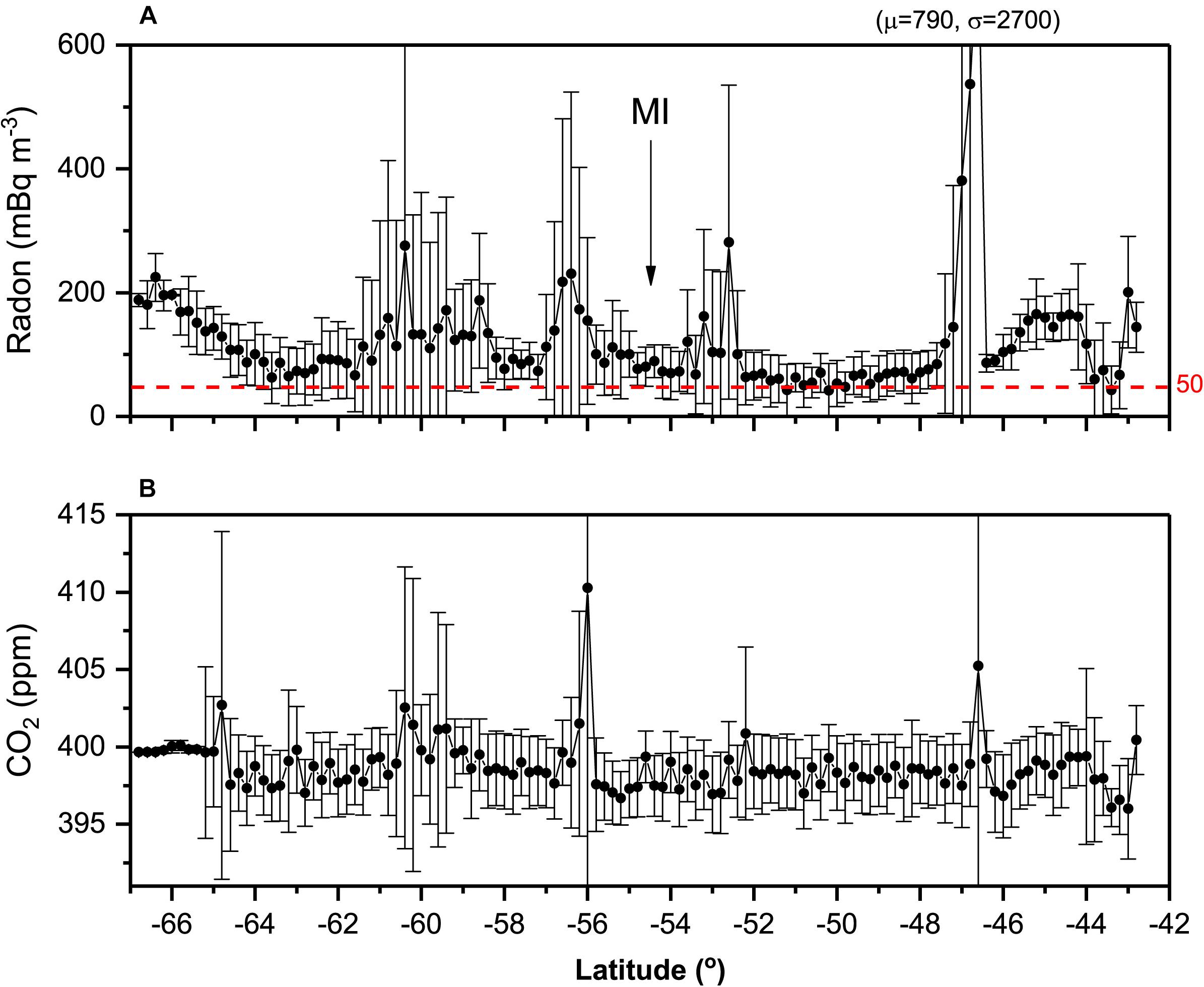
FIGURE 2. 5-track composite of (A) radon, and (B) carbon dioxide, concentrations (0.2° latitude bin means) between 45 and 67°S of Southern Ocean MBL. Whiskers represent ± 1σ. Approximate location of Macquarie Island is marked.
Between 49–51°S and 62–64°S average radon concentrations were close to 50 mBq m-3, indicative of minimal terrestrial influence within the past 2–3 weeks (i.e., marine “baseline” values, with radon in equilibrium with the Southern Ocean surface; Crawford et al., 2018 and references therein). By comparison, near the middle of this composite transect (i.e., 53–56°S) an enhancement of 30–40 mBq m-3 above baseline conditions was observed. Some previous studies have hypothesized that enhanced radon in the mid-Southern Ocean is entirely attributable to a wind-speed induced increase in the oceanic radon flux (e.g., Schery and Huang, 2004; Zahorowski et al., 2013). However, more recent evidence from an initial comparative baseline analyses of Cape Grim (Tasmania) and Macquarie Island air masses (Williams et al., 2017), suggests this radon enhancement is largely attributable to vestigial terrestrial influences on mid-Southern Ocean air masses. A detailed evaluation of this hypothesis will be the subject of a separate investigation. Notable similarities between Figure 2A and earlier transects reported by Polian et al. (1986) include higher concentrations around 60°S and at the Antarctic coast, with a local minimum in concentration around 63–64°S.
Several examples of isolated radon excursions from otherwise background conditions are evident in Figure 2A (e.g., at 46.5, 52.5, and 56.5°S). Back trajectories (HYSPLIT v4.0, Draxler and Rolph, 2003; using GDAS wind fields) indicated that contributing events were attributable to low-level (MBL) synoptic transport from Australia or New Zealand (e.g., Figure 3).
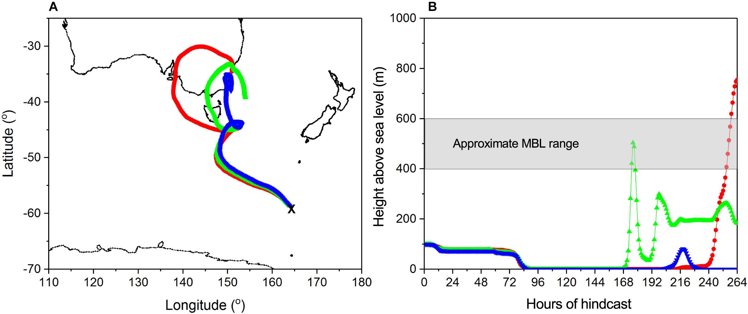
FIGURE 3. Back trajectories, (A) x-y and (B) x-z projections, associated with a mid-Southern Ocean radon enhancement event originating from south eastern Australia observed by the RV Investigator. Typical height range of the mid-Southern Ocean marine boundary layer inversion indicated.
The corresponding Southern Ocean CO2 transect (Figure 2B) shows enhancements associated with each of the three synoptic transport events identified in the radon record. Of equal interest, however, is the structure evident in the composite CO2 transect that is not associated with recent terrestrial influence (e.g., Stavert et al., 2018). This demonstrates the utility of high-quality shipborne radon observations in helping to isolate CO2 contributions arising from oceanic processes, terrestrial influences in excess of 3-weeks old or shipping exhaust.
A broad region of enhancement in both radon and CO2 is evident between 59 and 61°S. Back trajectories corresponding to the largest of these events (not shown) were not associated with synoptic MBL transport events, but were found to have recently descended from above the MBL. A mechanism for such transport events, postulated by Humphries et al. (2016), is terrestrially influenced free tropospheric air subsiding or intruding into the MBL in the vicinity of the circumpolar trough (“Polar Front”). This may provide further insight to high particle concentration events observed previously in the region (e.g., Humphries et al., 2015, 2016). Decay-correcting the observed radon concentrations based on modeled tropospheric transport times may provide a means of constraining the magnitude of the original terrestrial influence on the tropospheric air mass.
The last pronounced feature of Figure 2A is a “ramping” of radon concentration between 64 and 67°S (over ∼350 km). This increasing terrestrial influence on MBL air masses approaching the Antarctic coast in summer-autumn is attributable to two separate influences: a local Antarctic radon contribution from coastal exposed rocks (Evangelista and Pereira, 2002; Taguchi et al., 2013; Burton-Johnson et al., 2016; Chambers et al., 2017), and a remote terrestrial contribution within the outflow of tropospheric air masses that are descending over the Antarctic continent (Polian et al., 1986; Chambers et al., 2014, 2017). The fact that there is a step increase in CO2 within this same zone indicates that the outflow of subsiding tropospheric air is a large contributing factor, as the CO2 increase likely represents air that has not been in recent contact with the oceanic CO2 sink (Stavert et al., 2018). The ramping of radon concentrations may be partially a result of radioactive decay, indicating that the net northward movement of these outflowing air masses is quite slow (as expected of the strong easterly flow south of the circumpolar trough).
Seasonality of Terrestrial Influence in the Mid-Southern Ocean
Despite the isolation of MI (2000 km from mainland Australia, 1500 km from Tasmania, 1000 km from New Zealand), high radon concentrations (1500–3000 mBq m-3) were observed on average 4 times a year. Based on the conditions necessary to measure a significant (≥200 mBq m-3) local influence, i.e., a wind sector of 180–270° (Figure 1, inset 2) and wind speeds < 10 m s-1, less than 0.5% of events > 200 mBq m-3 in Figure 4A could be attributed to local island influences. When compared to radon in air masses leaving mainland Australia (50th – 75th percentile events 2000–4000 mBq m-3; Zahorowski et al., 2013), this indicates that it is possible for terrestrially influenced air masses to travel far into the Southern Ocean without substantial dilution.
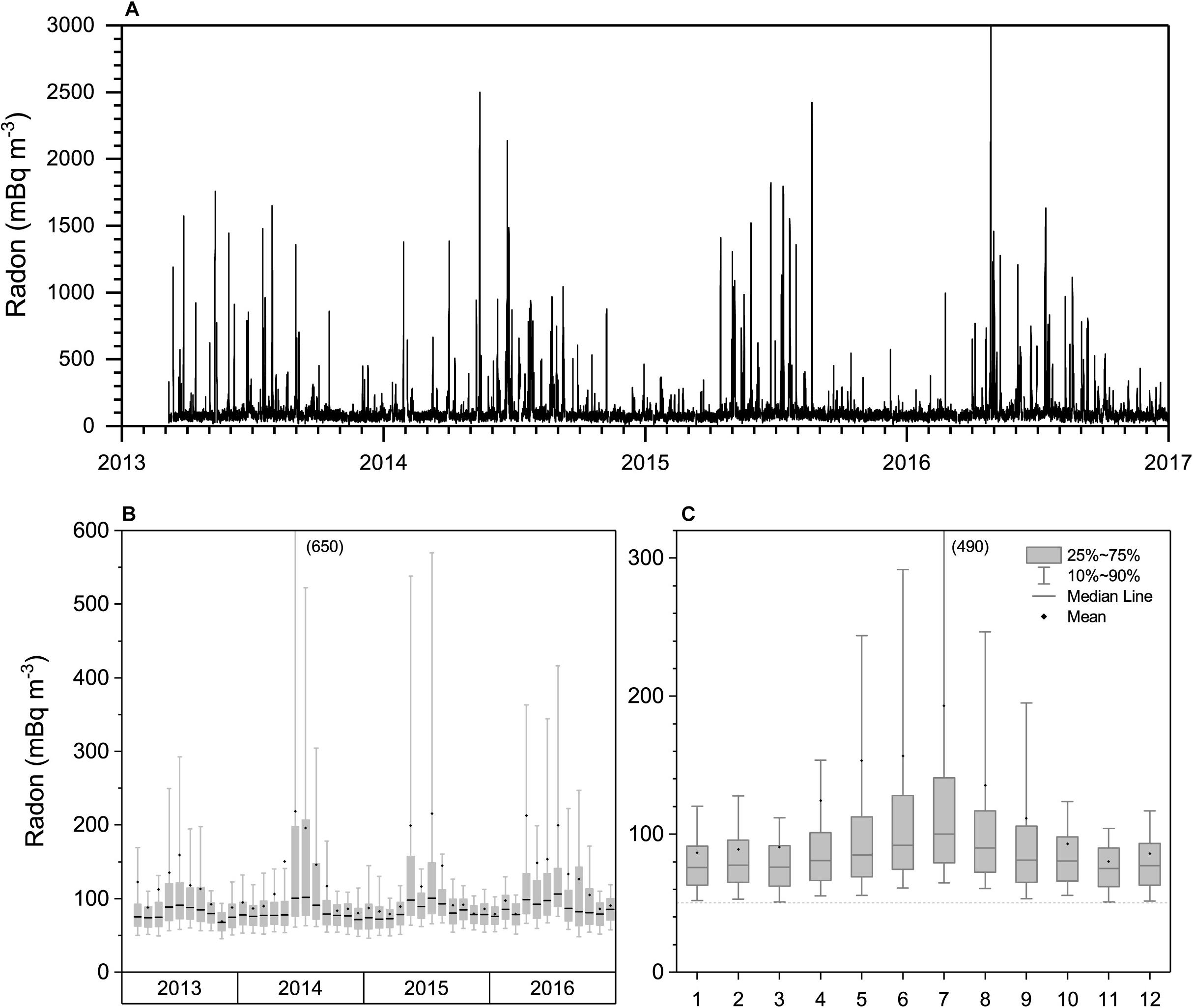
FIGURE 4. (A) Hourly, and (B,C) monthly distributions of radon concentrations at Macquarie Island based on a 4-year (2013–2016) composite of hourly observations. Refer to key for distribution box-plot details.
Monthly means and distributions of radon (Figures 4B,C) indicated a pronounced seasonal cycle characterized by a winter maximum and summer minimum. This cycle is thought to be largely attributable to the seasonal migration (north in winter, south in summer) of the surface divergence zone between the Hadley and Ferrel Cells (the “Subtropical ridge”), the average position of which is ∼30°S (see Figure 5 of Doering and Saey, 2014; Williams et al., 2017). Back trajectories calculated by Williams et al. (2017) indicated that even the seasonal cycle in the 10th percentile values is caused by vestigial continental influences.
To investigate possible wind speed influences on mid-Southern Ocean radon concentrations we calculated monthly wind speed distributions (not shown). The seasonal cycle, characterized by a broad March–October maximum (monthly median wind speeds of 10.3–11.3 m s-1) and November–February minimum (monthly median wind speeds 8.8–10.3 m s-1), had a low amplitude and did not match well with the seasonal radon cycle. Clearly, the seasonality of wind speed at this site is not the dominant influence on the seasonality in MBL radon concentrations.
Mean summer-autumn radon in the RV Investigator data at 54.5°S (Figure 2A) was 90–100 mBq m-3. This agrees well with the January–April monthly mean MI radon concentrations (Figure 4A). Agreement of mean concentrations within ∼10 mBq m-3 (i.e., ∼10%) between independently calibrated two-filter detectors provides confidence in comparisons drawn between other two-filter detectors in the Southern Ocean Network. Further confidence in the absolute radon concentrations reported by the RV Investigator is given by the estimate of 50 mBq m-3 for MBL air masses in the 49–51°S region of the Southern Ocean, as also reported by the independently operated 5000 L radon detector (LLD < 10 mBq m-3) at Cape Grim Station, Tasmania (Williams et al., 2017; Crawford et al., 2018).
It has already been demonstrated (Figure 2A) that minimum MBL radon concentrations in summer-autumn are higher toward the middle of the Southern Ocean than around 49 or 63°S. In addition, Figure 4C demonstrates that the magnitude of this enhanced terrestrial influence in the Southern Ocean varies seasonally, and is largest in winter.
Approaching the Antarctic Coast
In late summer 2017 (20-January to 25-February) the RV Investigator conducted a sea floor mapping exercise 200 – 400 km east of Casey Station, between about 50 and 150 km off the Antarctic coast (Figure 1, inset 1). Periods of considerable variability in trace atmospheric constituents and cloud condensation nuclei (CCN; TSI CPC Model 3776, size range > 3nm) were observed during this voyage. We investigate here whether they could be attributed to similar processes as the free-tropospheric particle events observed near the circumpolar trough (“Polar Front”) by Humphries et al. (2015, 2016).
This far offshore, little diurnal variability in MBL depth or radon concentration was expected given the ocean’s heat capacity, and the fact that the open ocean is a weak radon source without a diurnal cycle (Schery and Huang, 2004; Zahorowski et al., 2013), respectively. Over the course of the 37-day mission, however, amplitudes of the radon diurnal cycle varied from 0 to 50 mBq m-3 (Table 2). The amplitudes reported in Table 2 were calculated as the difference between 5-h means centered on the daily maximum and minimum hourly values.
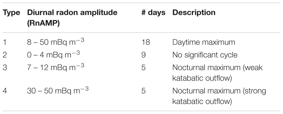
TABLE 2. Daily summary of MBL radon concentration characteristics observed from the RV Investigator between 20-January and 25-February 2017.
On some days the diurnal cycle was characterized by a daytime maximum and on others a nocturnal maximum (Table 2; Figure 5A). While the magnitudes of these diurnal cycles are 2–3 orders of magnitude lower than typically found at inland terrestrial sites (e.g., Chambers et al., 2015), the absolute accuracy of the two-filter detectors (<12% on a 1-h count for Rn > 100 mBq m-3; see Sites and Equipment), nevertheless provides confidence in the observed differences discussed below. Specifically, the uncertainty on each diurnal cycle amplitude (DU) is twice the uncertainty of the daily maximum or minimum estimate ; i.e., DU = 2(5.4%) = 10.8% ≈ 14 mBq m-3. While this level of uncertainty can’t guarantee clear distinction between type 2 and 3 events in Table 2, it is sufficient to distinguish type 1 and type 4 events, and each of these events from either type 2 or 3.
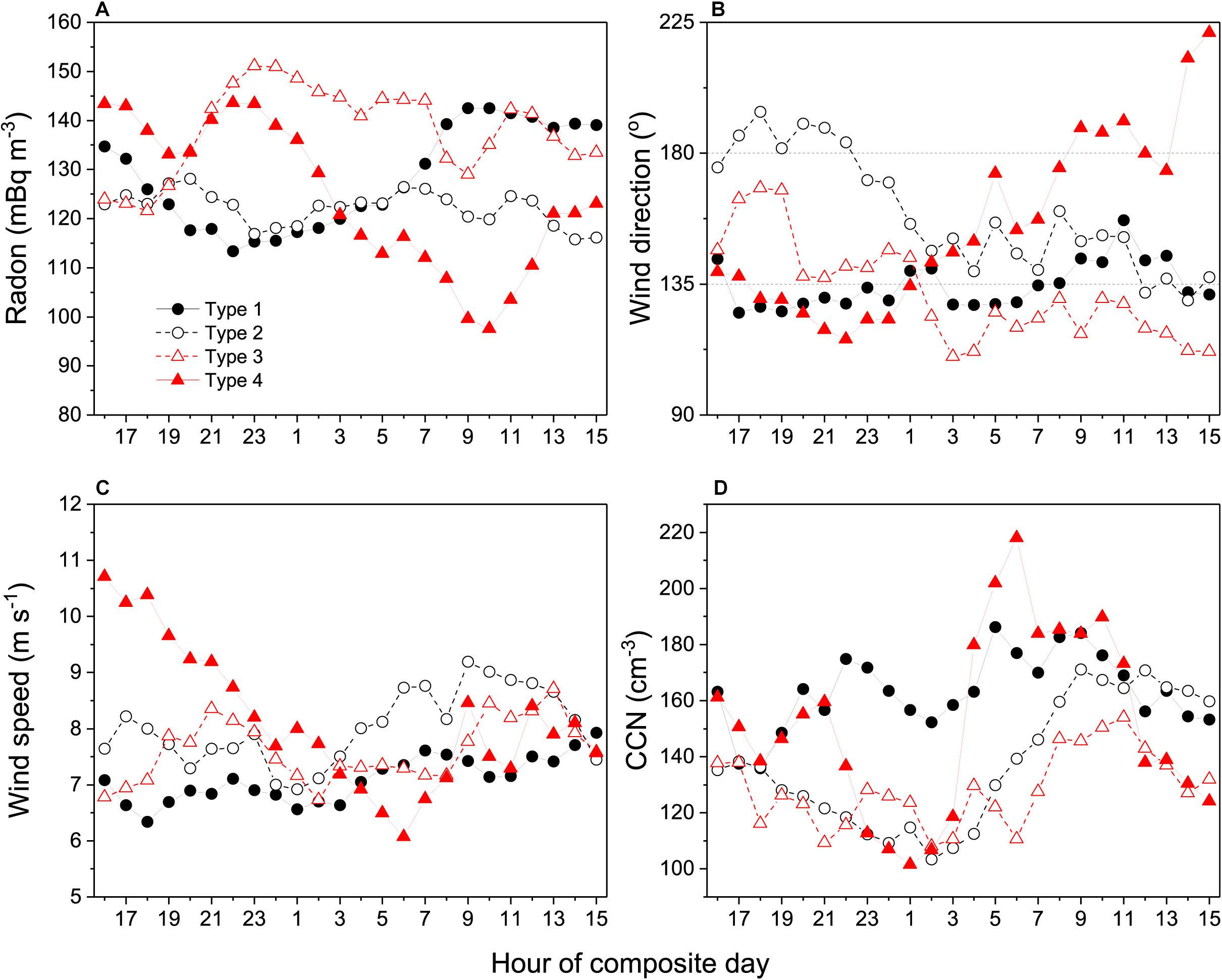
FIGURE 5. Diurnal composite (A) radon (means), (B) wind direction (medians), (C) wind speed (means), and (D) CCN (means across all supersaturation ranges; see Figure 6D), as observed from the RV Investigator for each day type described in Table 2. Time axis shifted to focus on the nocturnal period.
Type 1 days were characterized by daytime radon around 140 mBq m-3 (Figure 5A), wind directions from the southeast (Figure 5B; along the local coastline, Figure 1 inset 1), relatively consistent wind speeds (Figure 5C), and no pronounced diurnal cycle in CCN (Figure 5D). In this case the radon diurnal cycle amplitude (RnAMP = 25 mBq m-3) is likely attributable to changes in the coastal radon source function related to the diurnal freeze-thaw cycle, and this coastal air mixing to the local MBL (e.g., Bromwich et al., 1993). The January mean daily maximum and minimum coastal temperatures at Casey were +2.3 and -2.5°C, respectively.
Type 2 days had no consistent radon diurnal cycle and wind directions that changed from southerly to south-easterly, consistent with the passage of cyclonic synoptic systems. On overcast summer days coastal air temperatures typically peaked between -2 to 0°C, leading to less of a change in the coastal radon source function. Indeed, diurnal mean radon on these days was similar to the nocturnal concentrations for Type 1 days. The diurnal course of CCN on Type 2 days seemed to closely correspond to diurnal changes in wind speed and direction (oceanic fetch is more recent for south easterly air masses), indicating that salt spray was likely a dominant component of these aerosols.
Type 4 days were characterized by RnAMP = 46 mBq m-3, with a late morning minimum (Figure 5A). Until shortly after midnight the wind direction was roughly parallel to the coast and wind speeds were decreasing. From 0100 to 0200 h wind direction swung round to the south and southwest, almost perpendicular to the local coastline, and wind speeds increased by ∼3 m s-1. During this period, CCN increased to values higher than observed under the windiest conditions of Type 2 days, indicating that their origin is unlikely to relate to sea spray. Type 3 days shared many characteristics with Type 4 days, but to a lesser degree (reduced morning radon minimum, smaller and delayed morning peak in CCN).
In Figure 6 we investigate Type 4 days in more detail. Radon variability in the offshore flow (0400–1100 h) was lower than for periods of alongshore flow (Figure 6A). Air masses associated with offshore flow were also drier (Figure 6B). Ozone concentrations from 0400 to 1100 h were higher and less variable, and an increase was observed in all supersaturation ranges (0.25 – 1.05%) of CCN. The combination of timing, wind direction and air mass humidity suggest these morning events on Type 4 days are associated with katabatic outflow from the Antarctic mainland.
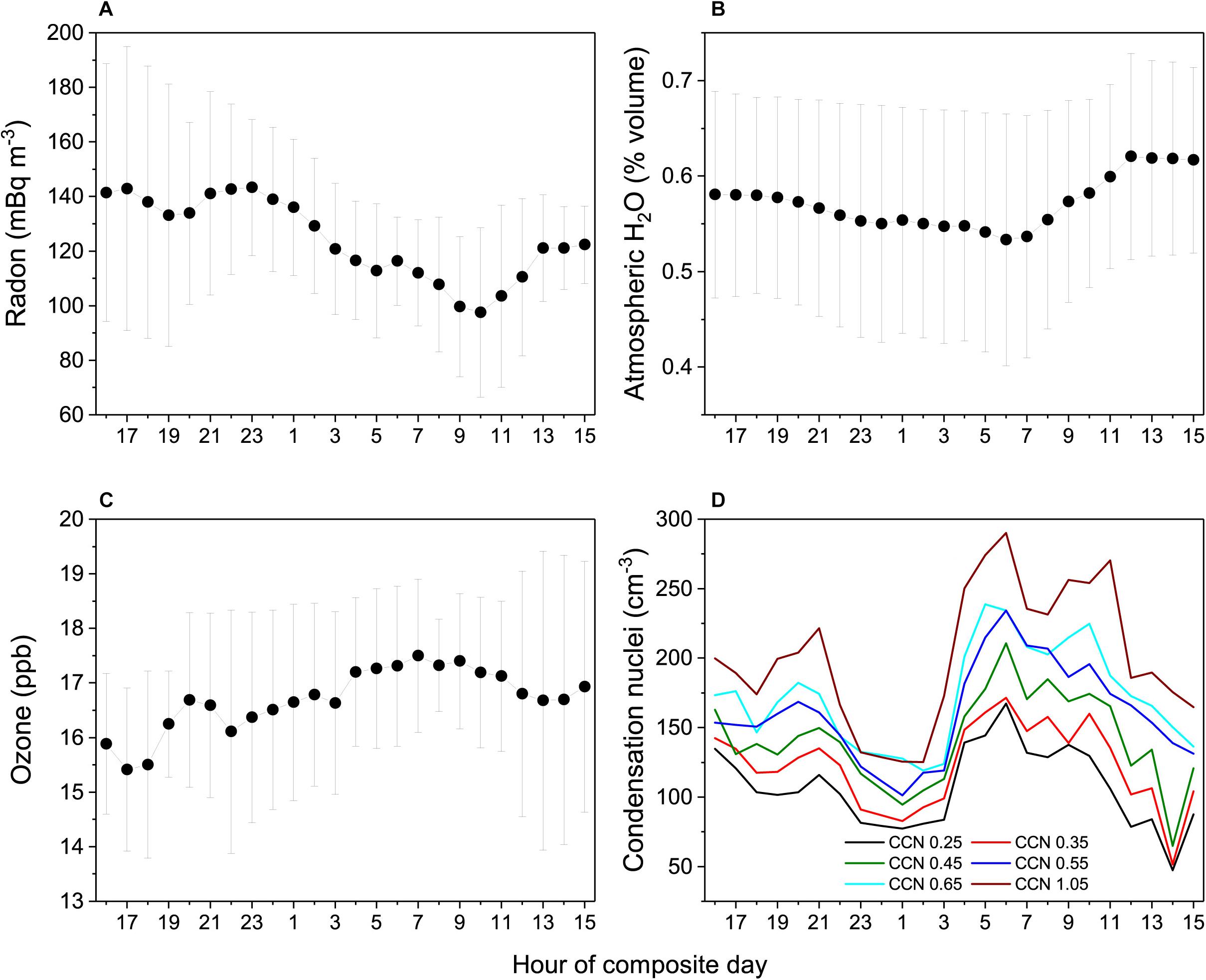
FIGURE 6. Diurnal composites of (A) radon, (B) % volume of water, (C) ozone, and (D) CCN (cm-3) within supersaturation ranges 0.25 – 1.05%, based on 5 days of katabatic outflow conditions. Whiskers represent hourly ± 1σ for the 5 days composite.
Since air within Antarctic katabatic flow events originates in the free-troposphere (Nylen et al., 2004), and crosses the coast at right angles (rather than traveling along or obliquely to it), there is a reduced opportunity for fetch across exposed rock, thereby reducing the average radon enhancement above “background” levels (30–50 mBq m-3) during outflow events. Having originated from the free-troposphere, these air masses also start out considerably drier than MBL air masses, and with higher ozone content. With their origin in mind, the observed increase in CCN of these recently tropospheric air masses is likely attributable to sulfate influences in the free-troposphere (Humphries et al., 2016; Obryk et al., 2018). In these regions the sulfate could be of anthropogenic, marine or volcanic origin (Graf et al., 2010). Related to these observations, Jaenickle et al. (1992) also reported an increase of CCN in subsiding tropospheric air at Neumayer station. As expected, back trajectories (not shown) confirmed that the free-tropospheric contributions to MBL air between 0400 and 1100 h on the outflow days of this study did not derive from the same tropospheric injection processes as those described by Humphries et al. (2016).
Five strong katabatic events in 37 days (Table 2), a relative frequency of ∼14%, is very similar to the 12% event frequency of pronounced katabatic flow in summer at Jang Bogo station reported by Chambers et al. (2017). The timing of the peak outflow was delayed by about 3 h compared to that of coastal events reported by Chambers et al. (2017), but this can be attributed to travel time based on the vessel’s distance from shore and the observed mean wind speeds of 8–9 m s-1.
The relatively weak contrasts in radon and humidity between katabatic outflow and MBL air masses shown in Figures 6A–C compared to the results of Chambers et al. (2017) and Section “Continental Antarctica” below indicate that considerable mixing (or ocean-atmosphere exchange) of the outflow air mass has occurred in transit to the RV Investigator. While this mixing prevents the reliable characterisation of tropospheric air in the outflow events in the way that can be achieved at coastal Antarctic sites (see Continental Antarctica), our findings clearly demonstrate that shipborne aerosol and trace gas measurements near the Antarctic coast should separately treat katabatic outflow days, or consider diurnal sampling windows, since the characteristics of recently tropospheric outflow air masses (i.e., potentially containing remote terrestrial influences) will not be representative of local conditions and may temporarily modify local ocean-atmosphere exchange processes.
Continental Antarctica
Coastal Sub-Antarctic (King Sejong Station: 62.2°S)
King Sejong Station is among the northernmost of the Antarctic bases (Figure 1), being about 500 km further north than most of the Antarctic coastline. Since the station is well removed from the topographic influences of the East Antarctic ice sheet, which reaches elevations above 4000 m a.s.l., of the Antarctic bases in this study KSG is best suited for year-round characterisation of marine baseline air masses of the remote Southern Ocean. In addition, the tip of the Antarctic Peninsula is also closer than any other part of continental Antarctica to another Southern Hemisphere continent (South America), so it also provides unique opportunities to observe the influence of recent direct transport of natural and anthropogenic terrestrial emissions to the frozen continent (e.g., Pereira, 1990; Pereira et al., 2004; Chambers et al., 2014).
Peak KSG radon concentrations (1500–2000 mBq m-3; Figure 7A) were lower than at MI, despite KSG being closer to South America than MI is to Australia. This is attributable to the combination of limited land fetch across South America (Pereira, 1990; Chambers et al., 2014), and high soil moistures in southern Chile.
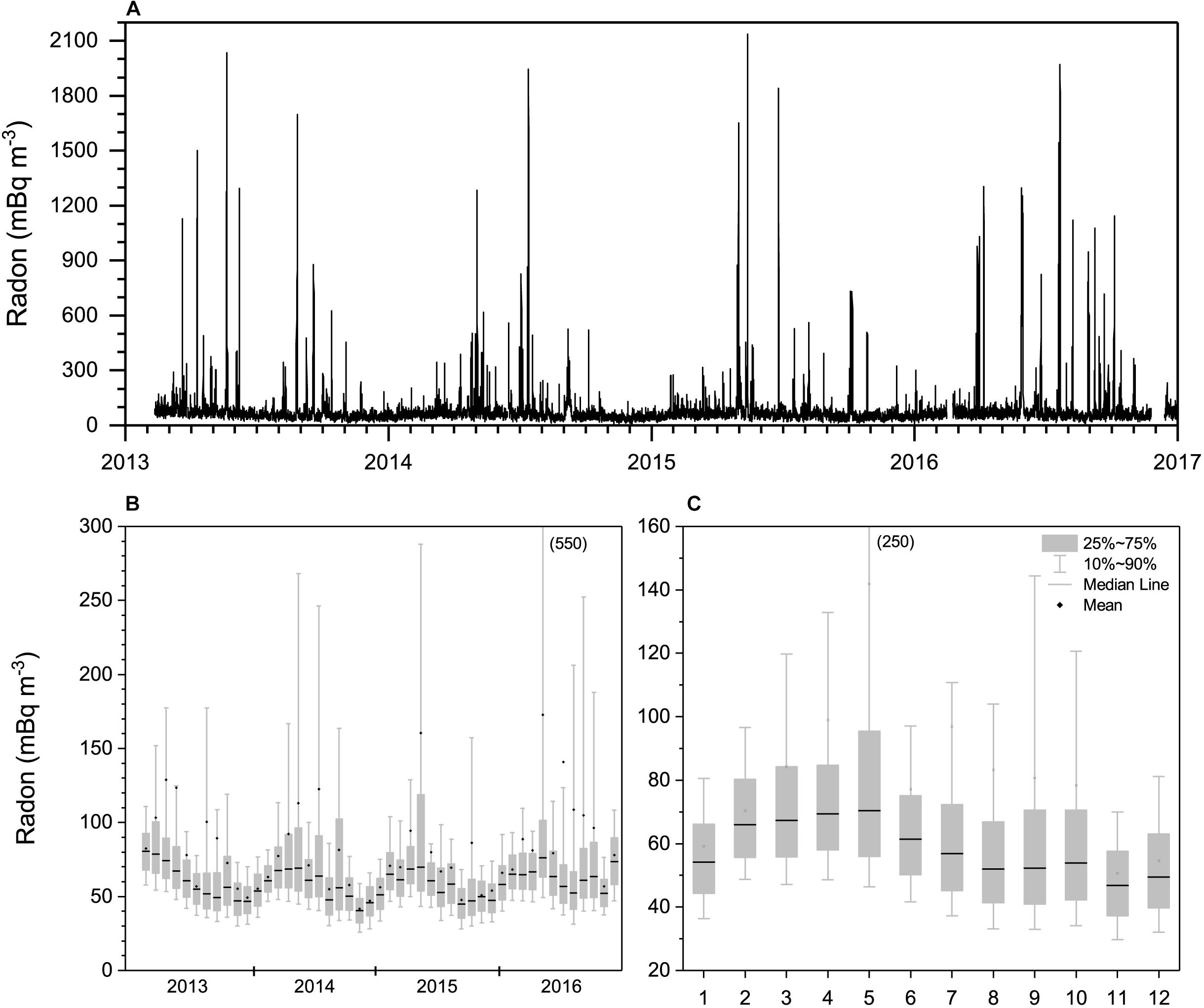
FIGURE 7. (A) Hourly, and (B,C) monthly distributions of KSG radon concentrations between 2013 and 2016. Refer to key for distribution box-plot details.
Summer median KSG radon concentrations were 50–55 mBq m-3 (Figures 7B,C), similar to the minimum 0.2° latitude bin mean values reported for this zone by the RV Investigator (Figure 2A), but lower than the corresponding MI values (75–80 mBq m-3; Figure 4C). This difference provides further independent confirmation of the small mid-Southern Ocean radon enhancement observed in the RV Investigator composite transect (Figure 2A). It should be noted here that, due to the station’s location (see Chambers et al., 2014), many KSG air masses with extensive oceanic fetch have to traverse at least ∼2 km of King George Island before reaching the site. Based on typical radon fluxes, mixing depths and wind speeds reported in Chambers et al. (2014), this terrestrial influence could enhance oceanic fetch radon concentrations by 5–10 mBq m-3.
The KSG radon seasonal cycle (Figures 7B,C) was quite distinct from that at MI. While minimum values were observed at both sites between November and January, peak values at KSG were bimodal, occurring in March-May and September–October. The latitude of KSG is close to the mean location of the circumpolar trough (convergence zone between the Ferrel and Polar Cells). Consequently, the seasonal migration of the circumpolar trough results in KSG switching between the influence of mid-latitude westerlies and Polar easterlies. In the non-summer months the synoptic cyclone track within the circumpolar trough is well located to bring air masses from the tip of South America to the station (Pereira et al., 2006 and references therein; Chambers et al., 2014).
Coastal Antarctica
Dumont d’Urville (66.7°S)
Two of the RV Investigator transects summarized in Section “The Southern Ocean in Cross-Section” approached the Antarctic coast near Dumont d’Urville (Figure 1). Inland from DDU the elevation reaches 2000 m a.s.l. within 200 km, before continuing up to >4000 m a.s.l. at the highest point of the Antarctic Plateau. Consequently, DDU is ideally situated to separately characterize long-term Southern Oceanic MBL air masses, as well as tropospheric air that has recently subsided over the Antarctic Plateau and comes down as katabatic flow events.
Peak DDU radon concentrations (180 – 275 mBq m-3; Figure 8) were an order of magnitude less than MI or KSG values, presumably because the nearest upwind non-frozen terrestrial fetch is 2500 – 3000 km away. However, the seasonal DDU radon cycle reported here (18 – 61 mBq m-3, based on monthly means), was also less than that reported by Polian et al. (1986) for DDU (25 – 65 mBq m-3), and less than the seasonal cycle at Mawson (67.5°S) (30 – 130 mBq m-3; Chambers et al., 2014). Furthermore, Ui et al. (1998) reported spring-summer daily mean radon concentrations at the coastal station of Syowa (69°S) between 150 and 270 mBq m-3. Potential factors contributing to this discrepancy have been discussed in Section “Sites and Equipment.”
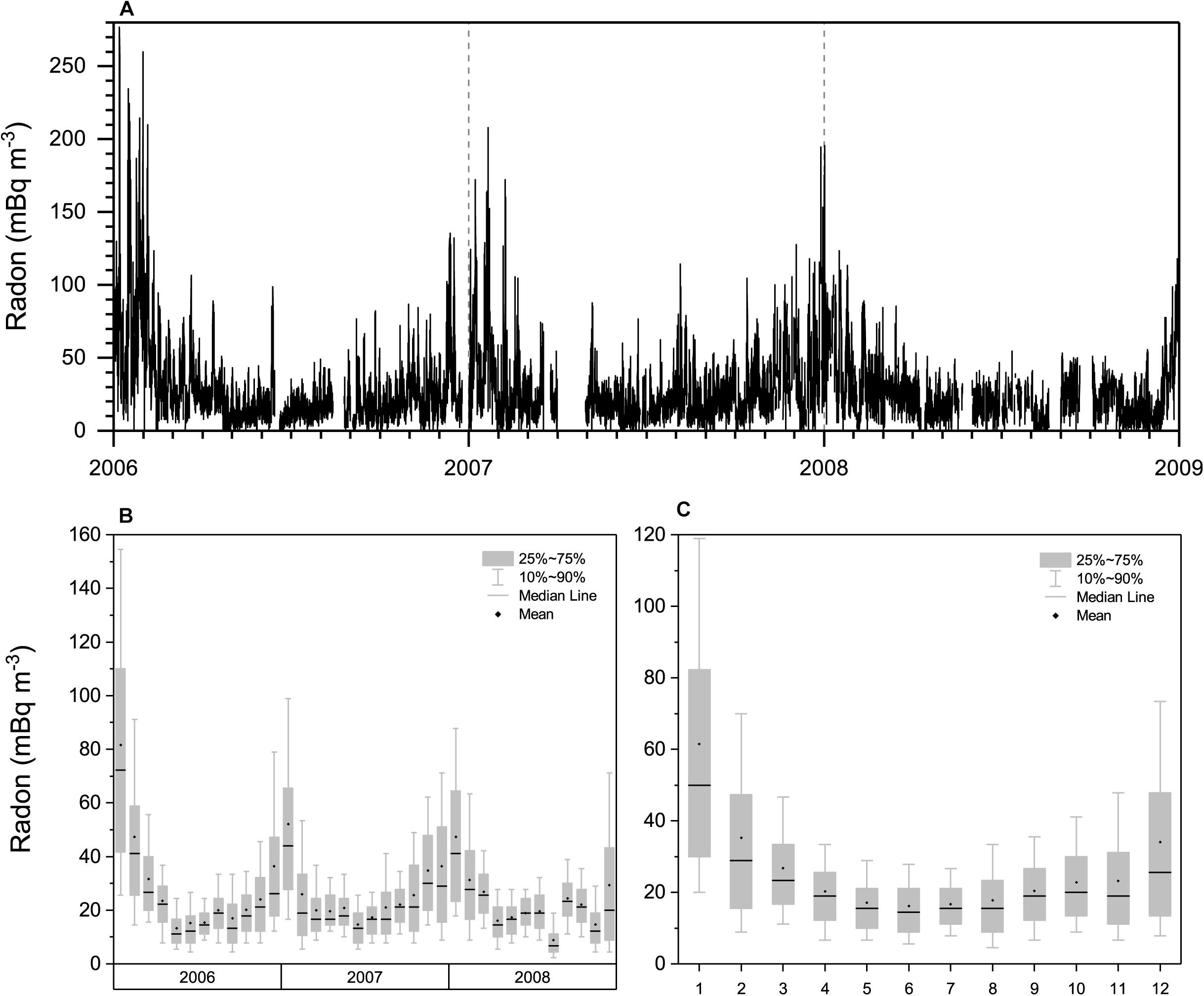
FIGURE 8. (A) Hourly, and (B,C) monthly distributions of DDU radon concentrations between 2006 and 2009. Refer to key for distribution box-plot details.
Similar to MI, the seasonal DDU radon cycle was unimodal, although peak concentrations occurred in mid-summer (Figure 8). Three factors are thought to have contributed to the summer increase in DDU radon concentrations: (i) the southward shift of the circumpolar trough permits passing cyclonic weather systems to bring air containing vestigial terrestrial influences from deeper within the Southern Ocean MBL directly to DDU; (ii) a greater amount of exposed rock and shallow coastal water at this time gives rise to an increased local radon flux from land and ocean; and (iii) tropospheric air descending over Antarctica in summer typically has experienced more recent terrestrial influence than corresponding winter air masses.
To further investigate these possible influences we employed a recently developed technique to separate air masses of different fetch at coastal East Antarctic sites (see Section 3.5 of Chambers et al., 2017). Here, the multi-year dataset was analyzed in 24-h blocks (defined from 1400 h to 1300 h the following day), each of which were assigned a category of “katabatic,” “local” or “oceanic” based on the mean 2-week high-pass filtered absolute humidity within an 8-h window (0000–0700 h) typically associated with katabatic flow. Days with the lowest 20% absolute humidity over this 8-h window are most likely to have experienced katabatic flow events. Days with the highest 20% absolute humidity over this 8-h window have experienced the most consistent oceanic fetch (i.e., arrived at the site most directly from the ocean). All remaining days (60% of the observations) were placed in the “coastal fetch” category (Figures 9A,B). Since the technique relies upon a measure of absolute humidity to assess fetch categories, as opposed to wind speed and direction or other meteorological quantities, it is capable of distinguishing between downslope flow that is truly katabatic, and downslope flow that has been synoptically forced.
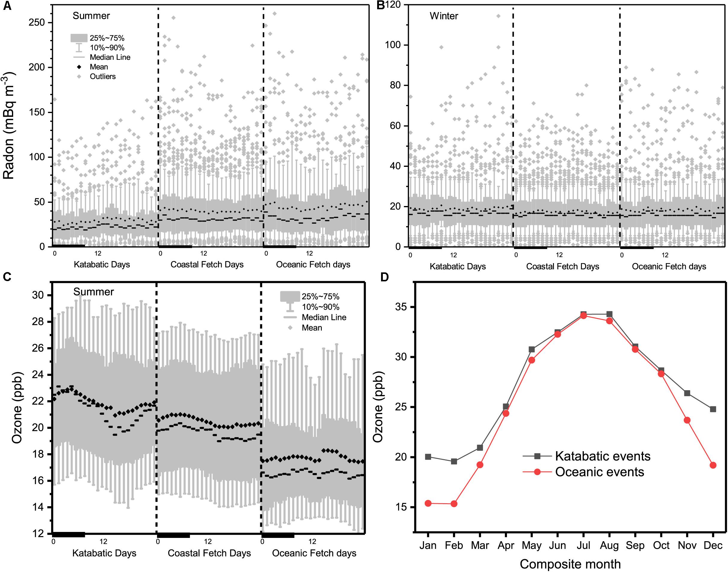
FIGURE 9. Diurnal composite (A,B) radon, and (C) ozone distributions, for days containing periods of katabatic, coastal and oceanic fetch at DDU, based on absolute humidity in the window 0000–0700 h (see text and plot key for details); (D) comparison of monthly mean ozone in katabatic and MBL air masses, at DDU based on observations from 2006 and 2008.
While results are presented here as full diurnal composites (0000 – 2300 h), the fetch analysis described above only strictly applies to the 0000–0700 h diurnal window, which has been marked with a bold line on each plot. Across the edges of the 24-h compositing window (i.e., between and close to the hours 1300–1400 h), discontinuities can arise due to edge effects of the compositing process (e.g., Figure 9C). Wind direction for oceanic fetch within the 8-h window was 110–120° and changed to 140–150° under katabatic conditions.
The highest mean DDU radon concentrations in summer (45–50 mBq m-3) occurred under oceanic fetch conditions (Figure 7A, RHS), consistent with expected radon concentrations for air in equilibrium with the Southern Ocean surface (30–50 mBq m-3; Zahorowski et al., 2013; Chambers et al., 2016). Outlier values of 90 – 265 mBq m-3 for these events indicate that oceanic air masses occasionally exhibit a vestigial terrestrial influence, likely attributable to long-range synoptic transport within the MBL (though possibly also related to subsidence near the circumpolar trough, see The Southern Ocean in Cross-Section).
On summer days, when coastal fetch prevailed in the 0000–0700 h diurnal window, mean radon concentrations were slightly lower (40–45 mBq m-3; Figure 9A, center), despite median values for oceanic and coastal events being almost identical. The reduced skewness of coastal events (90th percentile concentrations of 75–90 mBq m-3 compared with 95–100 mBq m-3 for oceanic events), is consistent with coastal events receiving low radon contributions from small, local coastal sources as discussed by Evangelista and Pereira (2002) and Chambers et al. (2014, 2017).
The lowest mean DDU radon concentrations in summer (24–29 mBq m-3) were associated with katabatic drainage events (from the free-troposphere/Antarctic Plateau). Unlike boundary layer air masses, free-tropospheric air masses have had an opportunity to be removed from all radon sources (terrestrial or oceanic) for a period of time, enabling them to achieve radon concentrations below even the 30–50 mBq m-3 associated with clean marine air. However, 10% of katabatic flow events (the marked outliers in Figure 9A, LHS) had radon concentrations between 55 and 165 mBq m-3, suggesting terrestrial influence within the past 2–3 weeks (ignoring dilution within the troposphere). Vertical profiles near DDU reported by Polian et al. (1986) also indicated an increase in radon concentrations from ∼15 mBq m-3 near the surface to ∼80 mBq m-3 between 2000 and 3000 m a.s.l., which is near the elevation of genesis for katabatic flow.
In summer there is ∼600 m of partially-exposed (∼50%) rock and soil to the south (inland) of DDU station (Preunkert et al., 2012). At speeds typical of katabatic flow (6–12 m s-1, gusting to 23 m s-1), even assuming a large radon flux (20 mBq m-2 s-1), and shallow mixing depths for these wind speeds (∼100 m), it is very unlikely that this fetch could contribute more than 10–15 mBq m-3 to the observed concentrations in the katabatic flow. Consequently, the bulk of the signal must arise from terrestrial influences within the tropospheric air.
Contrary to the summer results, the highest mean DDU radon concentrations in winter (Figure 9B) were in the katabatic flow events (18–21 mBq m-3; 27% lower than corresponding summer events). Peak concentrations of the winter katabatic events were 35–80 mBq m-3, indicating a summer-winter reduction in terrestrial influence on tropospheric air over DDU of almost a factor of two. Median winter radon concentrations of coastal and oceanic events were the same (∼16 mBq m-3), although mean values of the events coming most directly from the ocean were around 10% higher. The lower concentrations for coastal events are likely attributable to a greater air mass fetch time over ice, from which no radon is emitted, rather than open ocean, as previously mentioned by Weller et al. (2014) for radon observations at Neumayer Station. Based on baseline radon concentrations of 30–50 mBq m-3, and the 3.8-day radon half-life, winter “oceanic” DDU air masses have likely spent 4–6 days traveling over ice.
To demonstrate the ability of this technique to separately characterize dominant fetch regions of coastal Antarctic air masses, we briefly investigate some other DDU trace atmospheric constituents. Figure 9C compares diurnal composite summer ozone concentrations for katabatic, coastal fetch, and oceanic fetch days. Within the 8-h analysis window mean summer ozone concentrations were highest in katabatic flow (from the Antarctic Plateau) and lowest under oceanic fetch conditions.
The diurnal cycle of ozone at DDU was largest for days that experienced morning katabatic flow events (Figure 9C). The amplitude of this cycle was 2 (3) ppb based on hourly means (medians). These days typically experienced high radiation levels (e.g., Figure 10C) and lower mean wind speeds when averaged over the entire diurnal cycle. The ozone cycle was characterized by a mid-afternoon minimum and an early morning maximum at the time of peak katabatic flow, as evident in Figure 10A (black filled circles). Conversely, no consistent diurnal cycle was evident under oceanic fetch conditions (excluding the edge effect of the diurnal compositing procedure in the early afternoon). On coastal fetch days the amplitude of the diurnal ozone cycle was smaller, with the morning peak occurring a few hours later (Figure 9C, middle). Based on back trajectory fetch analyses Legrand et al. (2016) also found that ozone concentrations of air masses arriving at DDU in summer from the Antarctic interior were higher than those of oceanic air masses, in some cases by up to 10 ppbv.
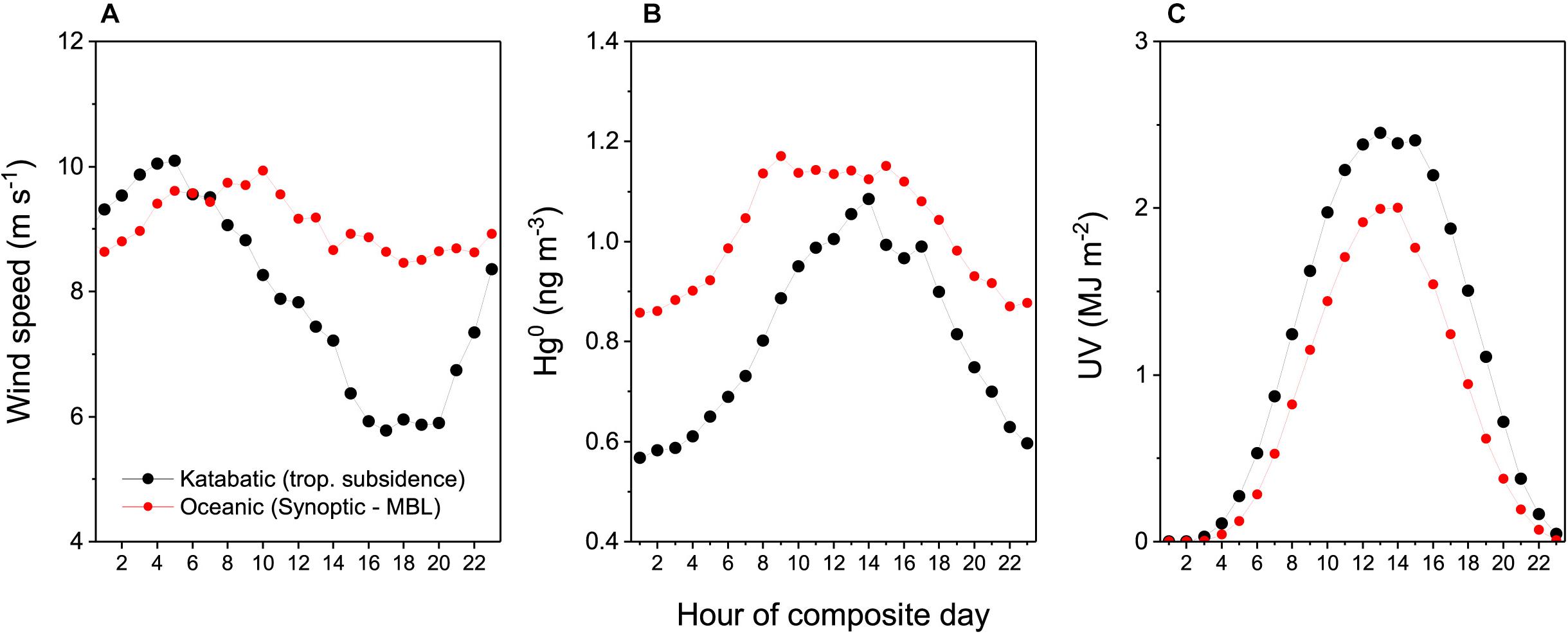
FIGURE 10. Diurnal composite (A) wind speed, (B) gaseous elemental mercury, and (C) ultraviolet radiation, at DDU (January-2012 to May-2015).
We calculated the daily mean ozone concentrations each month (using only observations within the 8-h analysis window) for katabatic flow and oceanic fetch events and prepared a 3-year composite (Figure 9D). In the summer months (November–February) we found that air descending from the Antarctic Plateau in katabatic flow events had monthly mean ozone concentrations around 5 ppb higher than oceanic air masses. The difference was much lower for the remainder of the year, but the tropospheric concentrations were always higher than those of oceanic air masses.
We processed a separate set of GEM observations at DDU (January-2012 to May-2015) in the same way to separate katabatic flow and oceanic fetch events (Figure 10). Mindful of possible temperature or UV-related GEM production in the coastal Antarctic environment (Angot et al., 2016c; Bargagli, 2016), we looked at the difference between summer mercury concentrations of katabatic flow and oceanic fetch events when UV levels were lowest (2300–0300 h; Figure 10C). We found that the katabatic flow was depleted around 0.3 ng m-3 in GEM compared to long-term oceanic air masses. This difference is of the same sign, but larger in magnitude, than that initially reported by Angot et al. (2016b) based on a back trajectory method of katabatic flow event identification. Based on estimated values of GEM in the Antarctic free troposphere of 0.9–1.0 ng m-3 [see Antarctic Plateau (Dome Concordia: 75°S, 3,233 m a.s.l.); and Song et al., 2018], the recently free-tropospheric katabatic flow events must have incorporated a large amount of air from the Antarctic Plateau where nocturnal GEM concentrations in summer are relatively depleted [Antarctic Plateau (Dome Concordia: 75°S, 3,233m a.s.l.); and Angot et al., 2016c].
The higher GEM concentrations in oceanic air at DDU are consistent with a combination of natural (including oceanic, especially in summer and fall) and anthropogenic sources of this long-lived (∼1 year residence time; Bargagli, 2016) gas. However, our estimated summertime oceanic GEM concentrations at DDU of ∼0.86 ng m-3 were slightly lower than summer concentrations reported at Troll Station (235 km inland of the Antarctic coast; 0.9 – 1.1 ng m-3), or at Italian Antarctic Station, Terra Nova Bay (74°41′S; 164°07′E) (0.9 ± 0.3 ng m-3) (Sprovieri et al., 2002, 2010; Dommergue et al., 2010), or Amsterdam Island (∼1.0 ng m-3) (Angot et al., 2014; Slemr et al., 2015; Sprovieri et al., 2016), consistent with observations at Cape Grim (Tasmania) and Singleton (NSW) (Slemr et al., 2015; Howard et al., 2017), but higher than reported by Kuss et al. (2011) for the southern Atlantic Ocean (0.72 ng m-3).
Neumayer (70.6°S)
Neumayer differs from most coastal Antarctic stations in that, instead of being built on rock, the station sits on the Ekström Ice Shelf, away from potential local sources of radon. Peak 3-hourly radon concentrations at Neumayer (110 – 155 mBq m-3; Figure 11A) were lower even than observed at DDU. While tempting to attribute these events to transport from South America, Weller et al. (2014) found little evidence for this. Rather, trajectory analyses often traced the origins of these events to the Antarctic interior. Ui et al. (1998) also reported high radon at Syowa station associated with southerly winds (from the Antarctic interior) and lower wind speeds (characteristic of anticyclonic conditions), but attributed this – we believe incorrectly – to unidentified local sources.
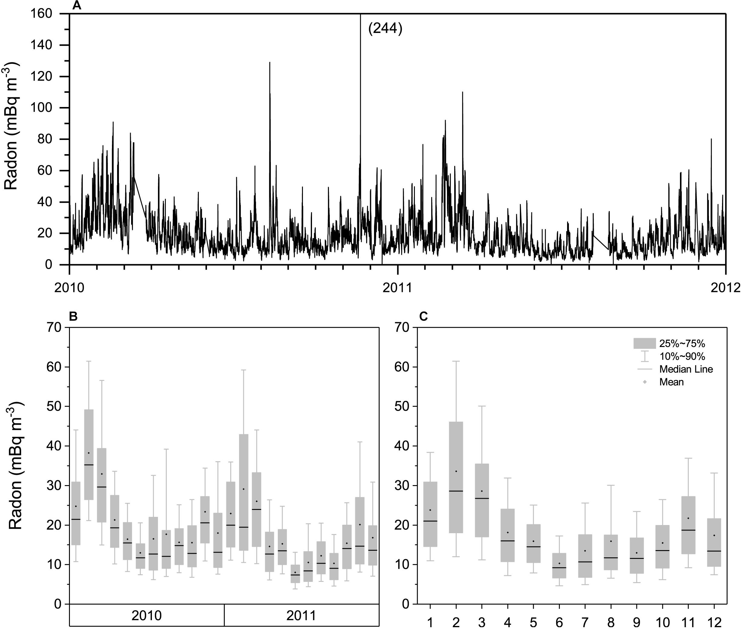
FIGURE 11. (A) Three-hourly, and (B,C) monthly distributions of NM radon concentrations for 2010 and 2011. Refer to key for distribution box-plot details.
As for KSG the NM seasonal radon cycle was bimodal, but with peak concentrations in February and November, and a pronounced mid-winter minimum (Figures 11B,C). Related to these observations, a strong seasonal cycle in CCN at NM has also been reported by Weller et al. (2011), characterized by a winter minimum and broad bi-modal maximum between September and April, peaking in March. Interestingly, the seasonal cycle of CCN at South Pole (considered to be attributable to largescale atmospheric transport processes in the free-troposphere; Samson et al., 1990), shares many features with the NM radon record (Figure 11C); including winter minimum, spring increase, reduced values in December and peak values in February through March.
Mean radon during katabatic outflow (27–30 mBq m-3) was higher than for oceanic fetch (20–22 mBq m-3) (Figure 12A), indicating more remote terrestrial influence in the Antarctic troposphere over NM than in the MBL air masses. Evidence of the katabatic nature of the events bringing the most recently tropospheric air to NM is given in the temperature and humidity plots of Figures 12C,D. Temperature and absolute humidity are extremely low for summer conditions during the suspected katabatic flow events, consistent with air originating in the free troposphere and passing over the Antarctic Plateau. Thus, most of the high radon events at NM are attributable to the subsidence of tropospheric air that has experienced recent (<3-week) terrestrial influence.
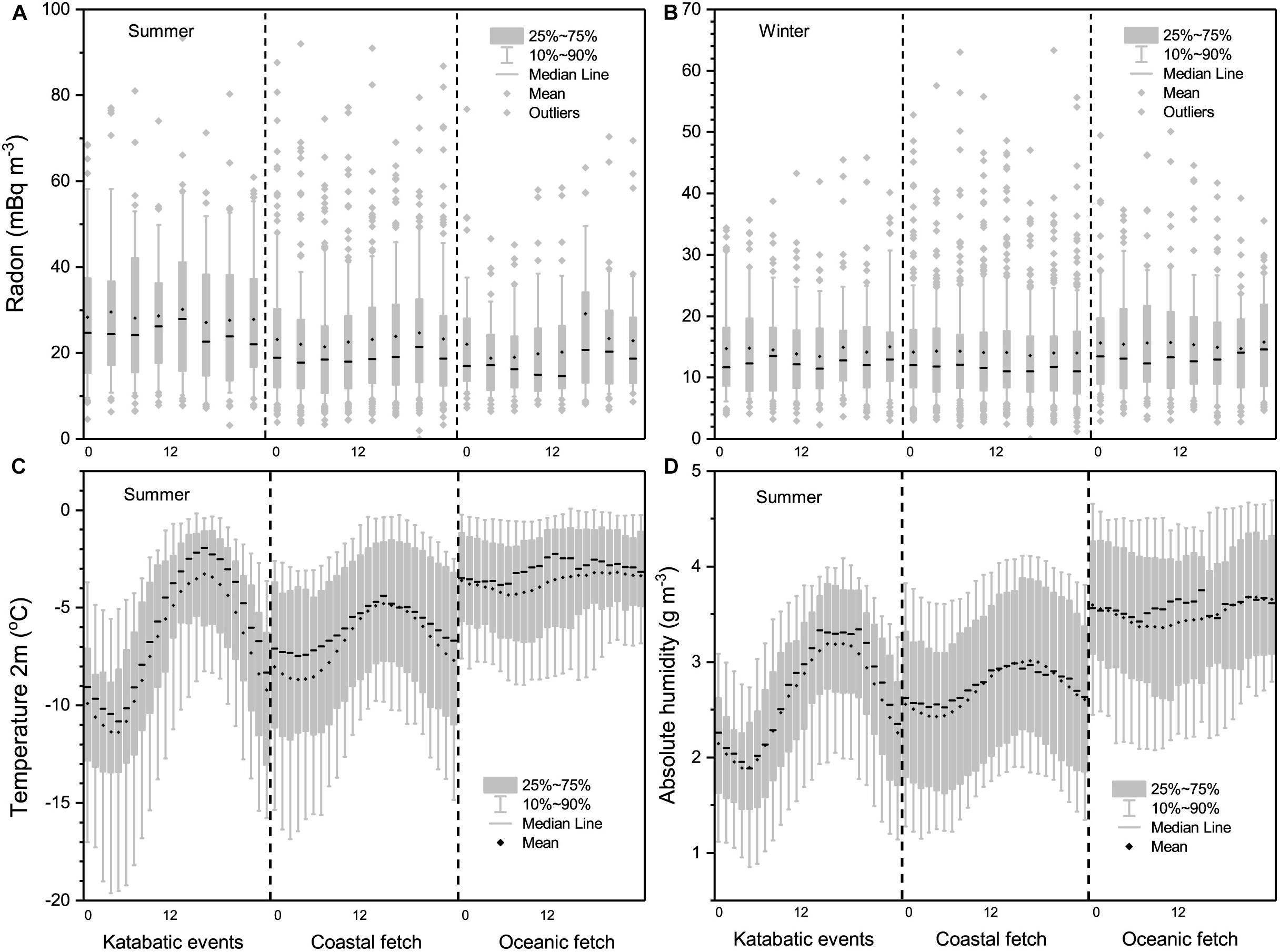
FIGURE 12. (A,B) Comparison of summer and winter diurnal composite radon distributions for katabatic, coastal and oceanic fetch, and (C,D) diurnal composite summer temperature and absolute humidity values for katabatic, coastal and oceanic fetch at NM in 2010 and 2011. Refer to key for distribution box-plot details.
In contrast to DDU, coastal air masses at NM have a lower mean radon concentration than the katabatic events. This is likely attributable to a smaller amount of exposed rock in the vicinity of NM (Weller et al., 2014). Also in contrast to DDU, oceanic air masses at NM have a lower mean radon concentration than those of katabatic air masses. This is attributable to a combination of more sea ice near NM (Weller et al., 2014; Legrand et al., 2016), and a reduced opportunity for significant recent terrestrial fetch for NM air masses.
The most extreme cases of recent terrestrial influence in the troposphere over Neumayer (55 – 90 mBq m-3) were considerably less than observed over DDU (55 – 170 mBq m-3). By contrast, the modeling studies of Li et al. (2008) and Albani et al. (2012) indicated a greater terrestrial influence in the free troposphere over NM than DDU. Clearly, further investigation is warranted of simulated terrestrial influence in Antarctica and the remote Southern Ocean (see also Discussion).
Outlier radon concentrations (45 – 90 mBq m-3) on days dominated by coastal fetch conditions indicate that coastal exposed-rock radon sources (“local” as in Antarctic, but remote from the station) can also influence observations at this site, but far less than at DDU. For days dominated by coastal fetch conditions a weak diurnal cycle (amplitude < 5 mBq m-3) was evident, but this was not significant given the variability of observations. No consistent radon diurnal cycle was observed on days that experienced morning katabatic flow events or predominantly oceanic fetch conditions (Figure 12A).
In summer, when sea ice extent is minimized, median radon concentrations for the most direct oceanic fetch conditions at coastal Antarctic sites should approximate the value for air masses in equilibrium with the Southern Ocean (i.e., 30–50 mBq m-3). At KSG, accounting for local fetch over King George Island [see Coastal Sub-Antarctic (King Sejong Station: 62.2°S)], median oceanic fetch radon concentrations in summer were 45–50 mBq m-3.
At DDU (Figure 7A) and NM (Figure 10A) median summer oceanic radon concentrations were 30–33 and 19–21 mBq m-3, respectively. The difference in median oceanic fetch radon concentrations between DDU and NM is believed to be largely attributable to sea ice in the vicinity of NM, some of which can still be present in summer. The 5–10 mBq m-3 difference between radon concentrations of oceanic air masses at DDU and those typical of the deep Southern Ocean MBL, on the other hand, might be attributable to tube loss of the sampled radon progeny (Levin et al., 2017). Given the short sample tube lengths at DDU, NM, and DC (see Sites and Equipment), this effect would not usually be significant, however, tube losses increase for radon concentrations < 1 Bq m-3, and at low ambient aerosol concentrations (when there can be a large unattached fraction of radon progeny; Levin et al., 2017). While tube loss effects at these sites have not yet been investigated, the possibility of a small (∼10–15 mBq m-3), possibly concentration-dependent, underestimation of radon concentrations by the HRMs in these extreme environments should be taken into consideration when interpreting reported free-tropospheric terrestrial influences (see also Sites and Equipment).
In winter there was little evidence of significant vestigial terrestrial influence in the free troposphere over NM (Figure 12B; LHS). Most of the larger winter radon events appeared to originate from coastal fetch events, including four events between 100 and 135 mBq m-3 that were not shown on Figure 12B to prevent compressing the scale of the plot. Mean radon for all winter air masses was well below the 30–50 mBq m-3 expected for oceanic air, which Weller et al. (2014) attributed to the extensive ice coverage in the region cutting off even the oceanic radon flux. Further evidence in support of this claim is that the mean concentration of radon in air masses coming most directly from the ocean in winter are slightly (∼8%) larger than air that has meandered around the Antarctic coastal regions.
Coastal/Interior (Jang Bogo, Terra Nova Bay: 75°S)
Jang Bogo (Chambers et al., 2017; and this study) and nearby Mario Zucchelli (Tositti et al., 2002), stations in Terra Nova Bay, are unique among all long-term Antarctic radon monitoring stations in their seasonal radon characteristics for two reasons: the amount of observed radon, and its source regions. Peak radon concentrations at these bases (3000 – 5500 mBq m-3; e.g., Figure 13A) are higher than observed at any other Antarctic Base, in some cases by more than an order of magnitude. Furthermore, as described by Tositti et al. (2002) and Chambers et al. (2017), the majority of this radon is from local Antarctic sources.
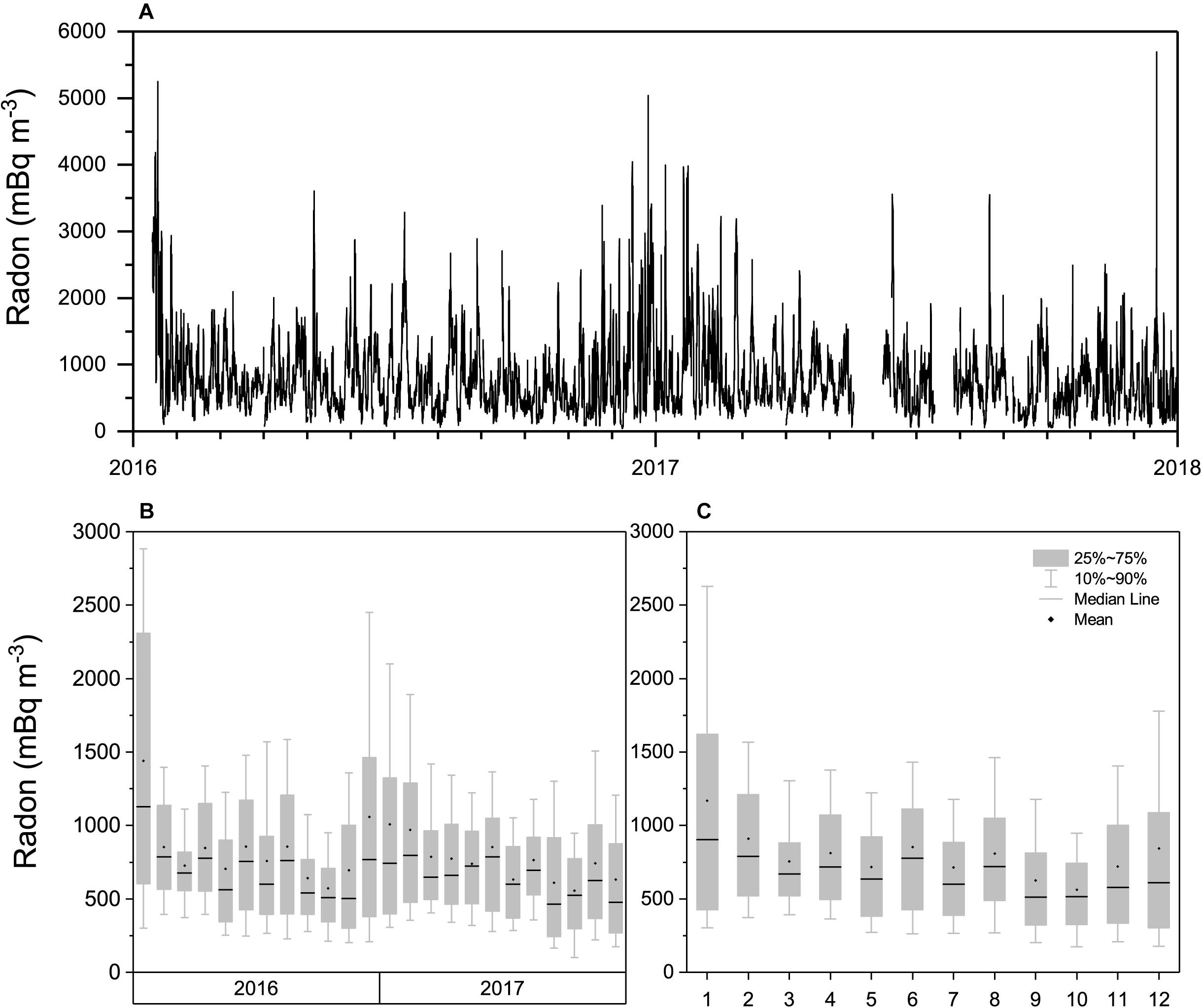
FIGURE 13. (A) Hourly, and (B,C) monthly distributions of JBS radon concentrations for 2016 and 2017. Refer to key for distribution box-plot details.
North and south of Terra Nova Bay, along the foothills of the Transantarctic Mountains, there is a substantial amount of exposed rock from which the mean summer radon flux has been estimated to be 0.09 – 0.11 atoms cm-2 s-1 (Chambers et al., 2017). The height and extent of the Transantarctic Mountains usually results in air masses approaching Terra Nova Bay from either the north or south, regardless of their longer-term fetch characteristics (e.g., katabatic outflow from the Ross Ice Shelf, barrier winds, and recent oceanic air masses – all from the south to southwest; or weaker anti-cyclonic flows from the north to northeast) (Markle et al., 2012; Coggins et al., 2014). As demonstrated by Markle et al. (2012) and Sinclair et al. (2013), even the freshest oceanic air masses are briefly redirected northward by the Transantarctic Mountains en route to Terra Nova Bay after moving from the Southern Pacific Ocean over the Ross Ice Shelf.
The combination of exposed rock fetch (100s of km in either direction), and relatively shallow mixing depths, frequently results in JBS radon concentrations of 1500–3000 mBq m-3 (Chambers et al., 2017). Additional radon sources, sometimes responsible for radon peaks > 4000 mBq m-3, include the active volcanos Mt Erebus and Mt Melbourne, along with their fumaroles (Polian and Lambert, 1979; Tositti et al., 2002).
The JBS seasonal radon cycle was not very consistent or pronounced in either mean or median values (Figures 13B,C). The most consistent features included a January maximum and October minimum. The seasonal cycle in 10th percentile values, on the other hand, was more consistent. This cycle was characterized by a February-April peak, consistent values throughout the winter months, and an October minimum.
Using the same 0000 – 0700 h diurnal analysis window as applied to observations at the other coastal Antarctic sites, 12% of summer days experienced pronounced katabatic flow events, and 18% of summer days experienced air mass fetch fairly directly from the ocean. The remaining 70% of summer days were classified as coastal fetch events (see Chambers et al., 2017, Section 3.5 for details).
As summarized in Figure 16 of Chambers et al. (2017), for brevity not repeated here, wind speeds of the summer oceanic fetch events were quite consistent, diurnal temperature amplitudes were low, and air masses made their final approach to the site from the southwest. Mean radon concentrations of these oceanic events were around 400 mBq m-3, an order of magnitude above typical marine baseline radon concentrations, due to the interaction of these air masses with the Transantarctic Mountains south of the station (Markle et al., 2012; Chambers et al., 2017). The modal summer radon concentration reported by Tositti et al. (2002) in this region was also 400 mBq m-3; with very few concentrations recorded below 200 mBq m-3.
By comparison, summer coastal fetch events had more variable wind speeds, typically approached from the north to northwest, and had radon concentrations around 900 mBq m-3, consistent with a longer fetch (∼330 km) along the foothills of the Transantarctic Mountains north of the site. In the case of summer katabatic flow events, at the time of peak katabatic wind speed (0200–0500 h) the composite mean radon concentration achieved a peak value of around 1000 mBq m-3. While a large contribution to this observed radon concentration from the local foothills of the Transantarctic Mountains can’t be ruled out (or accurately quantified), the katabatic flow is perpendicular to the mountain flanks so the air mass’ time over exposed ground is minimized (3–5 h as opposed to 1–3 days when coming from the north or south). Consequently, it is possible that 25–50% of the observed 900 – 1000 mBq m-3 of radon in katabatic flow events could derive from subsiding tropospheric air. This would mean that the troposphere over this part of Antarctica contained air of more recent terrestrial influence than that over DDU.
Antarctic Plateau (Dome Concordia: 75°S, 3,233 m a.s.l.)
Peak radon concentrations observed at the inland Dome Concordia Station (65–95 mBq m-3; Figure 14A), were the smallest of all Antarctic monitoring stations, and were restricted almost entirely to the summer months. The DC seasonal radon cycle (Figure 14B) was characterized by a February–March maximum, a September–October minimum, and relatively consistent concentrations between May and August; very similar to the 10th percentile seasonal cycle at JBS.
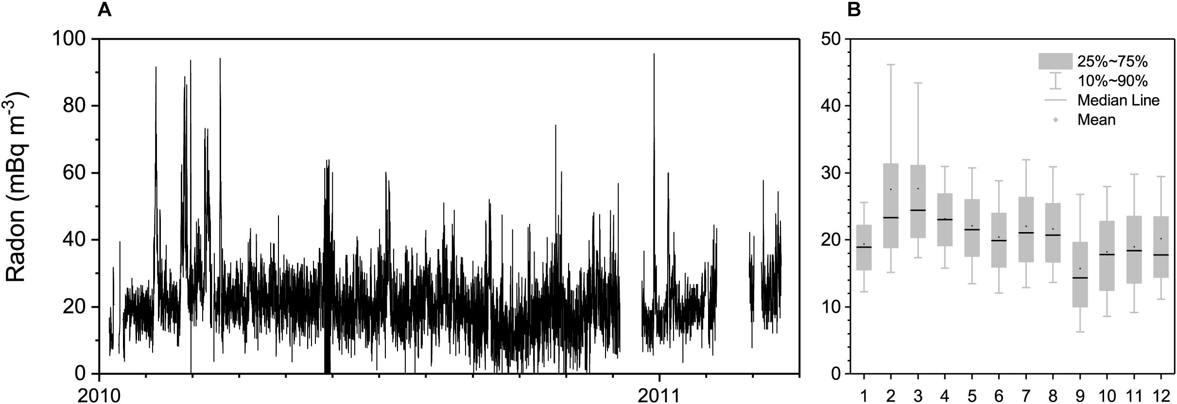
FIGURE 14. (A) Hourly, and (B) monthly distributions of radon concentrations at Dome Concordia in 2010. Refer to key for distribution box-plot details.
Unfortunately, no reliable humidity observations were available at the station for the 2010–2011 radon observation period. However, since subsidence events are usually strongest under anti-cyclonic conditions (clear-sky, light gradient winds), which usually also give rise to the greatest diurnal temperature variability at the surface, we approximated air mass type for these observations using surface temperature measurements.
We defined the diurnal temperature amplitude as the difference between 3-h means of the 2 m air temperature centered on the maximum and minimum observed hourly temperatures. We then calculated the diurnal amplitude of temperature for every day of the dataset and ranked these values for each season. Given that DC is cloud-free 75% of the time (Lawrence et al., 2004), we decided to categorize days with diurnal temperature amplitudes in the largest 33% as “anti-cyclonic,” those with the lowest 33% amplitudes as “strong advection,” and the remaining days were categorized as “weak advection.” Diurnal composite temperature plots for each of these 3 categories in summer are shown in Figure 15A.
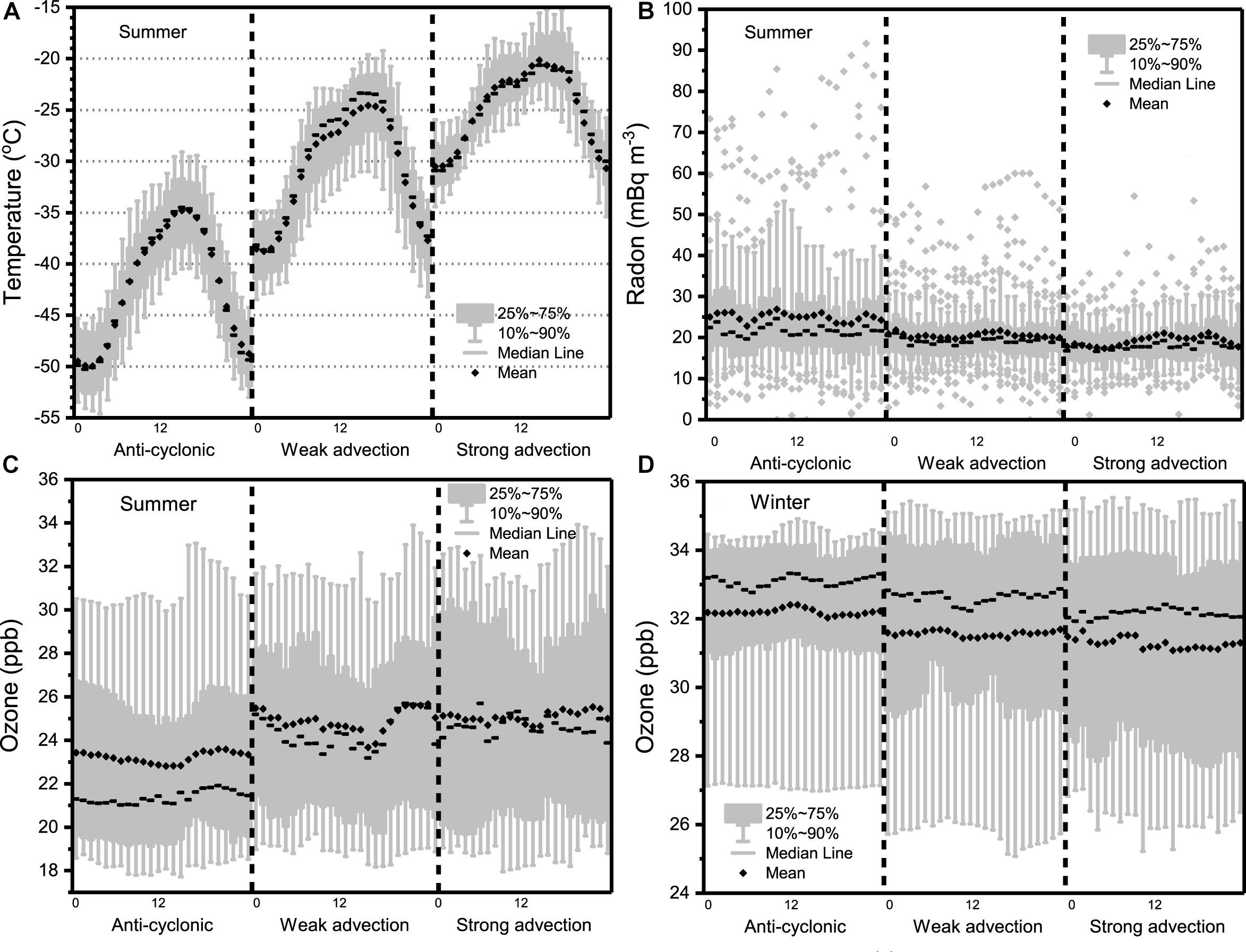
FIGURE 15. (A,B) Summer diurnal composite distributions of hourly temperature and radon at DC for the three fetch classes, and (C,D) summer-winter comparison of diurnal composite distributions of ozone at DC for the three fetch classes in 2010.
The highest mean DC radon concentrations in summer occurred on anti-cyclonic days (strongest subsidence; Figure 15B, LHS). Conversely, the lowest mean radon concentrations were observed on days when flow had been synoptically forced over the Antarctic interior (“strong advection” days). Almost all of the outlier events of magnitude 55 – 95 mBq m-3 were attributable to conditions during which the strongest tropospheric subsidence was thought to be occurring (anti-cyclonic conditions). It is notable that the radon concentrations observed for tropospheric subsidence events at DC compare well to those for “katabatic” conditions at both DDU and NM (22 – 33 mBq m-3), peaking at 55 – 90 mBq m-3.
We used the same fetch categorisation method to briefly examine the DC ozone record in summer and winter (Figures 15C,D). Median summer ozone for anti-cyclonic conditions (Figure 15C, LHS) was ∼21 ppbv, whereas corresponding winter values were 33 ppbv (Figure 15D, LHS). This is consistent with Legrand et al. (2009, 2016), who reported a seasonal cycle of ozone at DC characterized by a February minimum (∼21 ppbv) and July maximum (∼34 ppbv).
Anti-cyclonic days, in both summer and winter, were the only conditions under which consistent diurnal cycles of mean hourly ozone concentration were observed at DC. In summer the diurnal cycle was characterized by an early afternoon minimum. Legrand et al. (2016) demonstrate that daytime ozone minima on warm summer days at DC are attributable to increased boundary layer depths. In winter the diurnal cycle was characterized by a small noon maximum. In contrast to the case of summer the cause of this diurnal cycle in winter remains, however, basically unexplained.
In summer, the median ozone concentrations were 3 ppbv higher under strong advection conditions, when air masses were being synoptically forced over the Antarctic Plateau, than observed under subsidence conditions. Legrand et al. (2009, 2016) also report increased ozone concentrations at DC in summer when air is being advected to the site from other regions of the plateau. In winter, however, median ozone concentrations associated with strong air mass advection across the Antarctic Plateau were 1 ppbv lower than those observed under subsidence conditions.
In 2012–2013, when humidity measurements were available at DC, we separated daily air mass fetch conditions into tropospheric subsidence, local advection and strong advection (most recently oceanic) categories to investigate the source of the katabatic GEM depletion events observed at DDU (see Figure 10). In summer (Figure 16) we observed that air masses associated with direct tropospheric subsidence had 0000–0700 h mean GEM concentrations of 0.89 ± σ0.5 ng m-3, and those of air masses arriving most directly from the coast were 0.88 ± σ0.4 ng m-3. However, air masses that had been meandering locally about the Antarctic Plateau had average concentrations of 0.56 ± σ0.25 ng m-3, consistent with a strong summertime GEM sink on the Antarctic Plateau (Angot et al., 2016a,c; Wang et al., 2016) highlighting that the summertime removal mechanism of GEM is probably caused by other chemical processes than the springtime atmospheric mercury depletion events occurred in other polar areas. The higher variability of GEM concentrations in subsiding tropospheric air is likely attributable to changing levels of terrestrial influence, but radon observations were not available at DC in 2012–2013 to investigate this further.
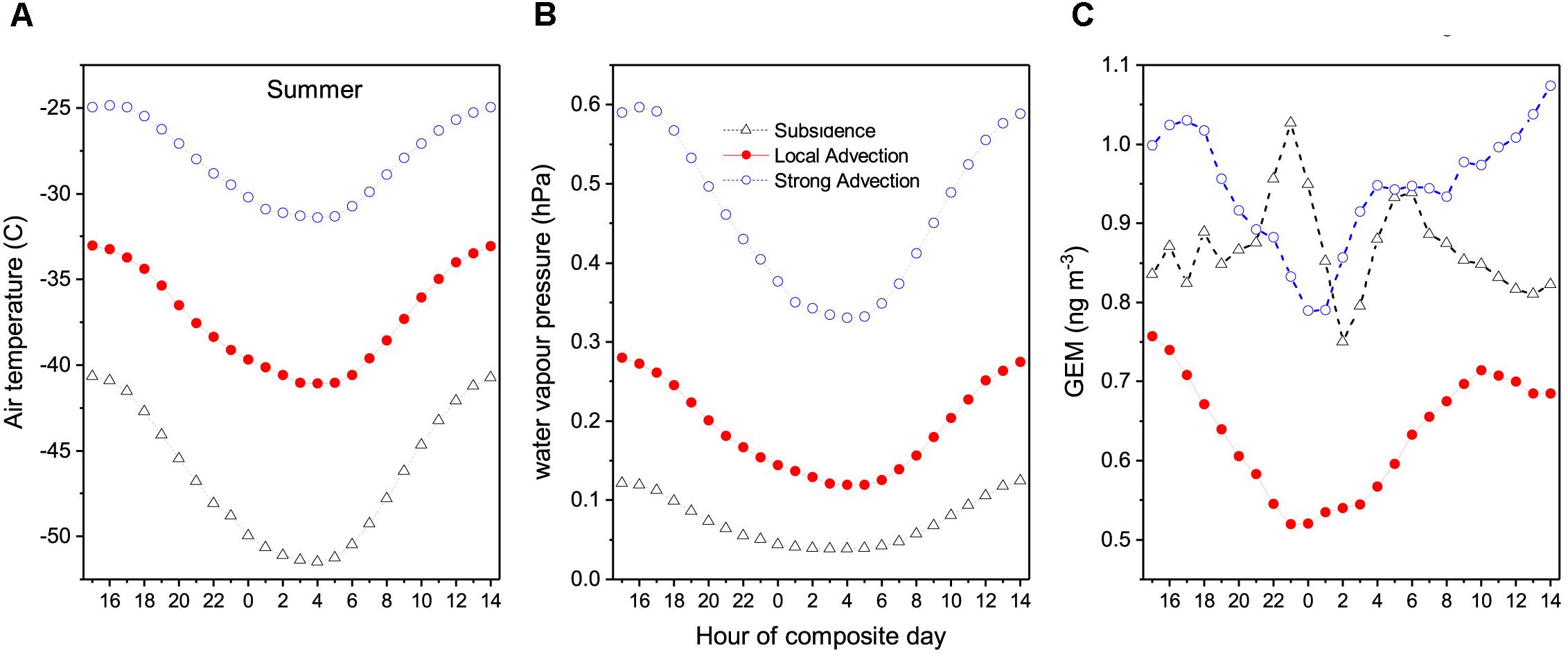
FIGURE 16. (A–C) Diurnal composite temperature, water vapor pressure, and GEM in summer for the three fetch categories in 2012–2013.
Discussion
Measurement Uncertainties and Historical Observations
Since this investigation sought to compare radon observations from numerous Southern Ocean/Antarctic sites made by independent instruments and measurement techniques, ideally a detector inter-comparison study should have been conducted first, in order to harmonize the results. However, since the datasets were collated retrospectively, this was not possible. As has been demonstrated by previous studies of this nature (Collé et al., 1996a,b; Schmithüsen et al., 2017), the value of instrument inter-comparisons should not be understated, rigorous calibration checks, particularly those performed “blind” with an independent referee, can shed considerable light upon expected or assumed performance.
As an example, Collé et al. (1996a,b) report on a 2-week inter-comparison of radon detectors performed in Bermuda (October 1991) including four participating laboratories, during which time ambient air was “spiked” 14 times with a Radon-222 sample of undisclosed activity. The measurement techniques compared included intermittent and continuous two-filter detectors, cryogenic separation using charcoal, and intermittent Radon-222 progeny collection on filters with equilibrium ratio assumptions. As noted by Collé et al. (1996b), both two-filter techniques “were in excellent agreement with the NIST [222Rn] additions.” In general, however, the continuous two-filter observations were overly smoothed by the detector’s 90-min time constant, changing particulate concentrations within the detector added considerably to the detector’s counting uncertainty, concentrations were initially overestimated by ∼10% (reduced to an overestimation of 2.7% only after a retrospective instrumental background correction), and there was considerable variability in concentrations at very low ambient radon levels, thought to be attributable to problems with instrumental background characterization.
The dual-flow-loop two-filter radon detectors employed in this study are based on the one originally tested in the Collé et al. (1996b) study, however, there have been considerable improvements to their design and performance in the 26 years since the Collé et al. (1996b) inter-comparison campaign. The original ANSTO two-filter radon detector design was superseded in the late 1990s by a completely new design involving the introduction of an innovation known as a “dual flow-loop” (Whittlestone and Zahorowski, 1998). Considerable additional improvements have been made since that time, as detailed in Chambers et al. (2014), Williams and Chambers (2016), Griffiths et al. (2016), and other articles. Williams and Chambers (2016), in particular, provide a detailed description of the progression of changes as realized for ANSTO two-filter detectors at the Cape Grim Baseline Air Pollution Station in Tasmania.
Briefly, key improvements to the two-filter detection systems in recent decades include: (i) the introduction of a second, high flow rate “internal” recirculation loop past the detection head, removing the need for a particle generator within the detector’s delay chamber to reduce plate-out losses of the newly formed radon progeny to the tank walls; together with a change of the main filter within the instrument sensing head from a coarse membrane filter to a 20 micron stainless steel mesh filter (enabled by the consequent change from predominantly particle-attached to unattached radon progeny within the tank), this has resulted in substantial increases in performance, consistency and reliability; (ii) a reduction in the instrument response time from 90 to 45 min; (iii) computer automation, which has enabled the performance of regular 3-monthly instrumental background checks and monthly system calibrations; and (iv) development of a response-time correction algorithm (Griffiths et al., 2016).
The lack of a formal evaluation of the performance of contemporary dual-flow-loop two-filter radon detectors is regrettable given the considerable discrepancy between Southern Ocean MBL radon concentrations reported at Cape Grim (e.g., Crawford et al., 2018) and in this study, and those reported in earlier Antarctic and sub-Antarctic studies, including that of Polian et al. (1986). Contemporary two-filter detector estimates of radon concentrations of air masses in long-term (≥3-week) equilibrium with the Southern Ocean based on observations at Cape Grim (Crawford et al., 2018), King Sejong Station, and aboard the RV Investigator, yield values typically between 40 and 50 mBq m-3. Furthermore, median summertime radon concentrations of oceanic air masses at Dumont d’Urville station measured by the single-filter method are around 30 mBq m-3 (prior to accounting for known tube-loss effects). Median Southern Ocean MBL radon concentrations reported by Polian et al. (1986), on the other hand, were around 15 mBq m-3. In order to determine which of these results is most representative, we sought to independently estimate MBL radon concentrations for the Southern Ocean region.
Assuming a uniformly mixed MBL, the radon concentration of oceanic air masses that have not been subjected to terrestrial influence in the past 3 weeks (RnMBL) can be estimated as follows:
where FRn_Oc is the oceanic radon flux (mBq m-2 s-1), we is the entrainment velocity (m s-1) across the MBL inversion, h is the depth of the MBL (m) and λ is the radon decay constant (2.0982 × 10⁻⁶ s-1). Average MBL depths near the northern extremity of the Southern Ocean (40–45°S) have been estimated to be around 900 – 1000 m (Zahorowski et al., 2013). Near the southern extremity (60–65°S) MBL depths have been estimated to be typically in the range 440 – 610 m (Chambers et al., 2014). Typical entrainment velocities for the Southern Ocean are of order 0.003–0.004 m s-1 (Zahorowski et al., 2013 and references therein). The seasonal variability of oceanic radon flux reported by Zahorowski et al. (2013) was in the range 0.19–0.34 mBq m-2 s-1, and other literature reviewed by Zahorowski et al. (2013) considered 0.24 mBq m-2 s-1 to be a generally representative oceanic radon flux.
Based on an entrainment velocity of 0.0035 m s-1 and an oceanic radon flux of 0.24 mBq m-2 s-1, for h = 1000 m, Equation (1) predicts RnMBL = 42.9 mBq m-3, whereas for h = 600 m, RnMBL = 50.4 mBq m-3. These estimates are in very good agreement with the Southern Ocean MBL radon concentrations reported in this study. Furthermore, with the notable exception of air masses recently mixed down from the free-troposphere or stratosphere that have been removed from all radon sources for a period of time, these findings indicate that the Southern Ocean MBL radon concentrations reported by Polian et al. (1986) are too low. The close agreement at very low ambient radon concentrations between independently calibrated two-filter radon detectors at Cape Grim (5000L model), aboard the RV Investigator (700L model), and at King Sejong station (1500L model), also provides confidence in contemporary methods to characterize the instrumental background compared to the two-filter detector that was employed in the Collé et al. (1996b) inter-comparison.
Comparison With Global Climate Model Simulations
A unique combination of physical properties (i.e., its source and sink terms, reactivity and half-life), makes radon an ideal tool to provide unambiguous information about terrestrial influence and transport mechanisms to remote Southern Ocean regions and Antarctica. Given the comparatively low land fraction of the Southern Hemisphere, it should provide an ideal “testing ground” for the performance of transport and mixing/convection parameterisations of global climate models (GCMs). Investigating spatial and temporal differences between observed and simulated radon concentrations throughout the Southern Hemisphere can provide significant insight to the behavior of GCMs.
A number of studies have successfully simulated synoptic radon transport in the MBL (sometimes called “radonic storms”) deep into the Southern Ocean (e.g., Balkanski and Jacob, 1990; Dentener et al., 1999). However, attempts by GCMs to reproduce the seasonal behavior of radon in coastal Antarctic regions have been far less successful (e.g., Heimann et al., 1990; Genthon and Armengaud, 1995; Taguchi et al., 2002; Josse et al., 2004; Zhang et al., 2008, 2011), which Josse et al. (2004) partly attributed to the paucity of reliable observational data. A summary of simulated radon seasonal cycles at Dumont d’Urville is presented in Figure 17.
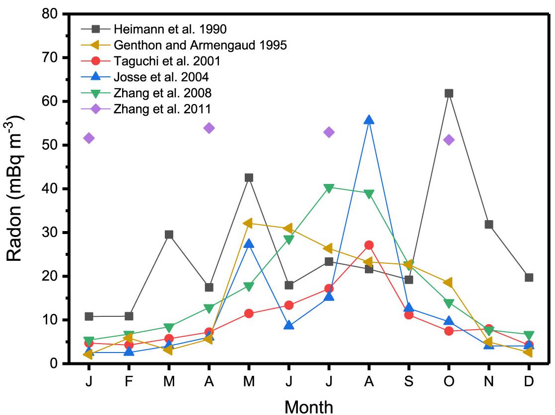
FIGURE 17. Monthly mean simulated radon concentrations at Dumont d’Urville for various years (see references for details).
The models of Genthon and Armengaud (1995), Taguchi et al. (2002), Josse et al. (2004), and Zhang et al. (2008) all produced a Dumont d’Urville radon seasonal cycle with a strong winter maximum and summer minimum. The phase of this seasonal cycle is completely opposite that of our observations at DDU (Figure 8C), but is similar to that observed at Macquarie Island (Figure 4C). With the exception of Heimann et al. (1990) and Zhang et al. (2011), similarities of the simulated seasonal cycle at DDU with MI observations indicate that these models are overestimating radon contributions at DDU that result from synoptic transport within the MBL. The complete failure to predict higher radon concentrations between November and February by these models is most likely mainly attributable to the fact that coastal radon sources in summer in Antarctica are not accounted for (see Figures 8C, 9A,B). Lastly, part of the higher observed radon concentration at DDU in January-February, and the sustained higher concentration into March, is likely attributable to the subsidence of tropospheric air containing vestigial terrestrial influence within the past 3 weeks. The models of Genthon and Armengaud (1995), Taguchi et al. (2002), Josse et al. (2004), and Zhang et al. (2008) all appear to have missed this contribution.
By comparison, Zhang et al. (2011) predict higher radon concentrations year round at DDU than the other models, and also at Mawson (not shown). However, the magnitude of these values compares reasonably well with oceanic radon concentrations in the lower parts of Southern Ocean observed by the RV Investigator (55–70 mBq m-3; Figure 2A), and median radon concentrations reported at KSG (50–70 mBq m-3). This similarity indicates that the Schery and Huang (2004) oceanic radon flux parameterisation used by Zhang et al. (2011) provides representative oceanic MBL radon values in that region of the Southern Ocean. The overestimation of radon concentrations in the winter months compared to observations at DDU and NM is likely due to a combination of (i) a slight underestimation of the observed radon concentrations by the HRMs at DDU and NM (see Sections “Sites and Equipment” and “Coastal Antarctica”), and (ii) an underestimation in the model of how much of the oceanic radon source function is “turned off” by the extensive winter ice sheet.
The amplitude of the seasonal radon cycle predicted by the Zhang et al. (2011) model (∼4 mBq m-3 at Dumont d’Urville, ∼15 mBq m-3 at Mawson) was, however, very low compared to observed values. The majority of this difference is likely attributable to a lack of consideration given to local Antarctic radon sources in the model (Evangelista and Pereira, 2002; Burton-Johnson et al., 2016; Chambers et al., 2017). Uniquely among the models compared here, the Zhang et al. (2011) seasonality predicts an autumn maximum concentration at Dumont d’Urville and a summer maximum at Mawson. Given that no account was made in these simulations for coastal Antarctic radon sources, this shift in phase of the radon seasonal cycle compared to the other models may indicate a more accurate representation of either the amount of continental air that is being injected to the mid-latitude troposphere, or the rate at which this air is subsequently traveling poleward.
Conclusion
We have discussed remote terrestrial influences on the boundary layer air masses over the Southern Ocean and Antarctica, as well as the mechanisms by which they arise, using continuous atmospheric radon (222Rn) measurements as a proxy. A composite of 5 Southern Ocean transects by the RV Investigator were used to provide a late-summer cross-sectional ‘snapshot’ of terrestrial influence in the marine boundary layer. These voyages provided considerable insight to tropospheric subsidence events occurring in the vicinity of the circumpolar trough, and the characteristics of outflow events that extend 100s of kilometers from the Antarctic continent.
The radon seasonal cycle at Macquarie Island, in the mid-Southern Ocean, was characterized by a summer minimum, winter maximum, and mean amplitude of ∼100 mBq m-3. Radon excursions beyond the 50 mBq m-3 marine background value were attributable to synoptic transport of continental air within the MBL. At King Sejong, in the sub-Antarctic, the radon seasonal cycle was bimodal with peaks in autumn and spring. Here radon excursions above background levels were contributed to by a combination of synoptic transport from South America, local radon sources, and subsidence of terrestrially influenced tropospheric air. Radon seasonal cycles at Dumont d’Urville and Neumayer Stations were dominated by local sources and tropospheric subsidence events, while that at Jang Bogo was primarily driven by local emissions. At Dome Concordia, far removed from coastal sources at 3,233 m a.s.l. on the Antarctic Plateau, the radon seasonal cycle was dominated by tropospheric subsidence events.
Separation of long-term marine and katabatic flow air masses was performed using a technique involving absolute humidity observations recently developed by Chambers et al. (2017). At Dumont d’Urville, this technique revealed monthly mean differences in ozone concentrations of around 5 ppbv in summer and 1 ppbv in winter. Averaged over a whole summer, concentrations of GEM were 0.03 ng m-3 lower in air masses that had recently subsided and traveled to the station from the Antarctic Plateau than in air masses of recent marine origin.
A comparison of our observations with simulated Antarctic radon seasonal cycles indicated that: (i) some models overestimate synoptic transport to Antarctica in the MBL, (ii) seasonality of the Antarctic ice sheet needs to be better represented, (iii) coastal Antarctic radon sources need to be taken into account, and (iv) the underestimation of radon in subsiding tropospheric air needs to be investigated.
The main purpose of this study was to bring together, and demonstrate the value of, seasonal high-sensitivity, high temporal resolution atmospheric radon observations from a number of contrasting locations in a growing network of Southern Ocean and Antarctic radon monitoring sites. By clearly demonstrating the cross-disciplinary benefits of an unambiguous indicator of terrestrial influence (or ‘potential pollution’) on MBL air masses throughout the Southern Ocean and coastal Antarctic regions, we hope to promote awareness, and encourage greater use of these datasets throughout the environmental research community. To assist with the interpretation of ongoing measurement programs, and continually improve the predictive ability of global models, every effort should be made to continue radon monitoring at existing stations, with a view to eventually making atmospheric radon observations a standard research measurement tool. However, given the low concentrations of radon typically present in remote Southern Ocean and Antarctic environments, and the range of measurement techniques and capabilities of contemporary detectors, further research in this field would greatly benefit from a detector inter-comparison campaign that specifically targeted concentrations approaching instrument detection limits.
Data Availability Statement
All source data of figures within this manuscript has been made available at the following location: 10.13140/RG.2.2.19918.92485 (https://www.researchgate.net/publication/327434026_Radon_concentrations_in_the_Southern_Ocean_and_Antarctic_regions). Regarding the RV Investigator in particular, meteorological data used was collected on the Marine National Facility (MNF) RV Investigator voyage IN2017_V01. The dataset in2017_v01uwy5min_csv.zip downloaded on 29-May-2018 was collected on voyage IN2017_v01 on the RV Investigator granted by the Marine National Facility. It is made available under a Creative Commons Attribution 4.0 International License; the data was processed by V. Dirita (CSIRO O&A). Data from the RV Investigator is available through the Earth Sciences section of the CSIRO Data Access Portal (https://data.csiro.au/dap/browse). Mercury data reported in this paper are available at https://gmos.aeris-data.fr/ (GMOS-FR Aeris database project) as well as within the central database of the GMOS global network at http://sdi.iia.cnr.it/geoint/publicpage/GMOS upon request. Radon measurements from the Air Chemistry Observatory at Neumayer Station are available from http://www.awi.de/en/go/air_chemistry_observatory). Meteorological observations from the Dome Concordia Automatic Weather Station (AWS 8989) of University of Wisconsin- Madison are available from ftp://amrc.ssec.wisc.edu/pub/aws/.
Author Contributions
SC, S-BH, and AW planned the study. SC installed the two-filter radon detectors and calibrated their observations, processed and interpreted meteorological and trace gas data from each site (provided calibrated and quality checked by co-authors), and drafted the initial manuscript. As well as roles played by many co-authors collecting data at field sites featured in this study, all co-authors actively contributed to revising and refining the interpretation of results presented. Additional contributions were as follows: SP and ML were responsible for meteorological, ozone and single-filter radon data from Dumont d’Urville and Dome Concordia. RW was responsible for meteorological and single-filter radon data from Neumayer. S-BH, TC, and LT provided meteorological data, and assisted with the collection of radon data, from King Sejong and Jang Bogo. RH, JS, SW, PK, SM, ZL, and IG were responsible for measurements of meteorology, carbon dioxide, ozone and condensation nuclei on the RV Investigator and at Macquarie Island. HA, OM, FS, NP, and AD were responsible for meteorology and GEM observations at Dumont d’Urville and Dome Concordia. AG and JC assisted with back trajectory calculation and figure production.
Funding
This research was partly supported by KOPRI research grants (PE18010) and The Australia Korea Foundation (AKF2014Grant00102). Atmospheric Hg measurements were supported by the FP7 (2010–2015) Global Mercury Observation System (GMOS) project. This work contributed to the EU-FP7 project Global Mercury Observation System (GMOS, www.gmos.eu) and has been supported by a grant from Labex OSUG@2020 (Investissements d’avenir – ANR10 LABX56). Logistical and financial support was provided by the French Polar Institute IPEV (Program 1028, GMOstral and Program 1011) and a grant from the U.S. National Science Foundation (NSF, PLR#1142145). The Automatic Weather Station Project, which supplied the meteorological parameters for Dome Concordia, is run by Charles R. Stearns at the University of Wisconsin-Madison and is funded by the National Science Foundation of the United States of America.
Conflict of Interest Statement
The authors declare that the research was conducted in the absence of any commercial or financial relationships that could be construed as a potential conflict of interest.
Acknowledgments
We thank over-wintering staff at all contributing Antarctic stations, and crew of the RV Investigator, for their part in maintaining the radon, meteorological and other equipment from which data has been gathered for this study. In particular we wish to thank Ot Sisoutham and Sylvester Werczynski, of ANSTO, for their support of the radon measurement program. Field logistic supplies for the Rn measurements at DDU and DC were provided by Institut Polaire Français-Paul Emile Victor (IPEV) within program 414. We thank Météo France, who provided meteorological data for DDU, and Charles R. Stearns for the Automatic Weather Station Project that provided meteorological parameters for Dome Concordia. We thank LEFE/IMAGO programs CLAPA and GABLS4, IPEV CALVA program 1013 (PI: Christophe Genthon), and Observatoire des Sciences de l’Univers de Grenoble (GLACIOCLIM observatory) for providing meteorological data for 2012–2013 in Concordia station. We gratefully acknowledge the Air Resources Laboratory (ARL) for provision of the HYSPLIT transport and dispersion model on READY website (https://ready.arl.noaa.gov/HYSPLIT_traj.php) used in this publication. Last but not least, we would also like to thank the reviewers for their insightful and constructive feedback, which has helped improving the clarity and utility of the final manuscript.
Footnotes
References
Albani, S., Mahowald, N. M., Delmonte, B., Maggi, V., and Winckler, G. (2012). Comparing modeled and observed changes in mineral dust transport and deposition to Antarctica between the Last Glacial Maximum and current climates. Clim. Dyn. 38, 1731–1755. doi: 10.1007/s00382-011-1139-5
Amante, C., and Eakins, B. W. (2009). ETOPO1 1 Arc-Minute Global Relief Model: Procedures, Data Sources and Analysis. NOAA Technical Memorandum NESDIS NGDC-24. Silver Spring, MD: NOAA. doi: 10.7289/V5C8276M
Angot, H., Barret, M., Magand, O., Ramonet, M., and Dommergue, A. (2014). A 2-year record of atmospheric mercury species at a background Southern Hemisphere station on Amsterdam Island. Atmos. Chem. Phys. 14, 11461–11473. doi: 10.5194/acp-14-11461-2014
Angot, H., Dastoor, A., de Simone, F., Dastoor, A., De Simone, F., Gårdfeldt, K., et al. (2016a). Chemical cycling and deposition of atmospheric mercury in polar regions: review of recent measurements and comparison with models. Atmos. Chem. Phys. 16, 10735–10763. doi: 10.5194/acp-16-10735-2016
Angot, H., Dion, I., Vogel, N., Legrand, M., Magand, O., and Dommergue, A. (2016b). Multi-year record of atmospheric mercury at Dumont d’Urville, East Antarctic coast: continental outflow and oceanic influences. Atmos. Chem. Phys. 16, 8265–8279. doi: 10.5194/acp-16-8265-2016
Angot, H., Magand, O., Helmig, D., Ricaud, P., Quennehen, B., Gallée, H., et al. (2016c). New insights into the atmospheric mercury cycling in central Antarctica and implications on a continental scale. Atmos. Chem. Phys. 16, 8249–8264. doi: 10.5194/acp-16-8249-2016
Australian Antarctic Division (2005). Macquarie Island and Adjacent Islands 1:50000 Coastline GIS Dataset. Available at: https://data.gov.au/dataset/e4c01f74-de78-4233-80f4-444dfdc7380b
Balkanski, Y. J., and Jacob, D. J. (1990). Transport of continental air to the Subantarctic Indian Ocean. Tellus 42B, 62–75. doi: 10.3402/tellusb.v42i1.15192
Bargagli, R. (2016). Atmospheric chemistry of mercury in Antarctica and the role of cryptogams to assess deposition patterns in coastal ice-free areas. Chemosphere 163, 202–208. doi: 10.1016/j.chemosphere.2016.08.007
Belikov, D. A., Maksyutov, S., Krol, M., Fraser, A., Rigby, M., Bian, H., et al. (2013). Off-line algorithm for calculation of vertical tracer transport in the troposphere due to deep convection. Atmos. Chem. Phys. 13, 1093–1114. doi: 10.5194/acp-13-1093-2013
Brechtel, F. J., Kreidenweis, S. M., and Swan, H. B. (1998). Air mass characteristics, aerosol particle number concentrations, and number size distributions at Macquarie Island during the First Aerosol Characterisation Experiment (ACE 1). J. Geophys. Res. 103, 16351–16367. doi: 10.1029/97JD03014
Bromwich, D. H., Parish, T. R., Pellegrini, A., Stearns, C. R., and Weidner, G. A. (1993). Spatial and temporal characteristics of the intense katabatic winds at Terra Nova Bay, Antarctica. Antarct. Res. Ser. 61, 47–68. doi: 10.1029/AR061p0047
Brook, E. J., and Buizert, C. (2018). Antarctic and global climate history viewed from ice cores. Nature 558, 200–208. doi: 10.1038/s41586-018-0172-5
Brunke, E.-G., Labuschagne, C., Parker, B., Scheel, H. E., and Whittlestone, S. (2004). Baseline air mass selection at Cape Point, South Africa: application of 222Rn and other filter criteria to CO2. Atmos. Environ. 38, 5693–5702. doi: 10.1016/j.atmosenv.2004.04.024
Burton-Johnson, A., Black, M., Fretwell, P. T., and Kaluza-Gilbert, J. (2016). An automated methodology for differentiating rock from snow, clouds and sea in Antarctica from Landsat 8 imagery: a new rock outcrop map and area estimation for the entire Antarctic continent. Cryosphere 10, 1665–1677. doi: 10.5194/tc-10-1665-2016
Chambers, S., and Sheppard, S. C. (2017). Letter to the editor. J. Environ. Radioact. 172, 261–263. doi: 10.1016/j.jenvrad.2017.04.013
Chambers, S. D., Choi, T., Park, S. J., Williams, A. G., Hong, S.-B., Tositti, L., et al. (2017). Investigating local and remote terrestrial influence on air masses at contrasting Antarctic sites using Radon-222 and back trajectories. J. Geophys. Res. Atmos. 122, 13525–13544. doi: 10.1002/2017JD026833
Chambers, S. D., Hong, S.-B., Williams, A. G., Crawford, J., Griffiths, A. D., and Park, S.-J. (2014). Characterising terrestrial influences on Antarctic air masses using Radon-222 measurements at King George Island. Atmos. Chem. Phys. 14, 9903–9916. doi: 10.5194/acp-14-9903-2014
Chambers, S. D., Williams, A. G., Conen, F., Griffiths, A., Reimann, S., Steinbacher, M., et al. (2016). Towards a universal “baseline” characterisation of air masses for high- and low-altitude observing stations using radon-222. Aerosol Air Qual. Res. 16, 885–899. doi: 10.4209/aaqr.2015.06.0391
Chambers, S. D., Williams, A. G., Crawford, J., and Griffiths, A. D. (2015). On the use of radon for quantifying the effects of atmospheric stability on urban emissions. Atmos. Chem. Phys. 15, 1175–1190. doi: 10.5194/acp-15-1175-2015
Coggins, J. H. J., McDonald, A. J., and Jolly, B. (2014). Synoptic climatology of the Ross ice shelf and Ross Sea region of Antarctica: k-means clustering and validation. Int. J. Climatol. 34, 2330–2348. doi: 10.1002/joc.3842
Collé, R., Unterweger, M. P., Hodge, P. A., and Hutchison, J. M. (1996a). An international marine-atmospheric 222Rn measurement intercomparison in Bermuda Part I: NIST calibration and methodology for standardized sample additions. J. Res. Natl. Inst. Stand. Technol. 101, 1–19.
Collé, R., Unterweger, M. P., and Hutchison, J. M. (1996b). An international marine-atmospheric 222Rn measurement intercomparison in Bermuda Part II: results for the participating laboratories. J. Res. Natl. Inst. Stand. Technol. 101, 21–46.
Crawford, J., Chambers, S. D., Cohen, D. D., and Williams, A. G. (2018). Baseline characterisation of source contributions to daily-integrated PM2.5 observations at Cape Grim using Radon-222. Environ. Pollut. 243, 37–48. doi: 10.1016/j.envpol.2018.08.043
Crawford, J. H., Davis, D. D., Chen, G., Buhr, M., Oltmans, S., Weller, R., et al. (2001). Evidence for photochemical production of ozone at the South Pole surface. Geophys. Res. Lett. 28, 3641–3644. doi: 10.1029/2001GL013055
Davis, D., Nowak, J. B., Chen, G., Buhr, M., Arimoto, R., Hogan, A., et al. (2001). Unexpected high levels of NO observed at South Pole. Geophys. Res. Lett. 28, 3625–3628. doi: 10.1029/2000GL012584
DeConto, R. M., and Pollard, D. (2016). Contribution of Antarctica to past and future sea-level rise. Nature 531, 591–597. doi: 10.1038/nature17145
Dentener, F., Feichter, J., and Jeuken, A. (1999). Simulation of the transport of Rn222 using on-line and off-line global models at different horizontal resolutions: a detailed comparison with measurements. Tellus 51B, 573–602. doi: 10.3402/tellusb.v51i3.16440
Doering, C., and Saey, P. (2014). Hadley cell influence on 7Be activity concentrations at Australian mainland IMS radionuclide particulate stations. J. Environ. Radioact. 127, 88–94. doi: 10.1016/j.jenvrad.2013.10.011
Dommergue, A., Sprovieri, F., Pirrone, N., Ebinghaus, R., Brooks, S., Courteaud, J., et al. (2010). Overview of mercury measurements in the Antarctic troposphere. Atmos. Chem. Phys. 10, 3309–3319. doi: 10.5194/acp-10-3309-2010
Draxler, R. R., and Rolph, G. D. (2003). Hybrid Single-Particle Lagrangian Integrated Trajectory (HYSPLIT), Model. Available at: http://www.arl.noaa.gov/ready/hysplit4.html [accessed September 2016].
Eisele, F., Davis, D. D., Helmig, D., Oltmans, S. J., Neff, W., Huey, G., et al. (2008). Antarctic tropospheric chemistry investigation (ANTCI) 2003 overview. Atmos. Environ. 42, 2749–2761. doi: 10.1016/j.atmosenv.2007.04.013
Etheridge, D. M., Steele, L. P., Langenfelds, R. L., Francey, R. J., Barnola, J.-M., and Morgan, V. I. (1996). Natural and anthropogenic changes in atmospheric CO2 over the last 1000 years from air in Antarctic ice and firn. JGR Atmos. 101, 4115–4128. doi: 10.1029/95JD03410
Evangelista, H., and Pereira, E. B. (2002). Radon flux at king George island, Antarctic peninsula. J. Environ. Radioact. 61, 283–304. doi: 10.1016/S0265-931X(01)00137-0
Fox, A. J., Paul, A., and Cooper, R. (1994). Measured properties of the Antarctic Ice Sheet derived from the SCAR Antarctic Digital Database. Polar Res. 30, 201–206. doi: 10.1017/S0032247400024268
Genthon, C., and Armengaud, A. (1995). Radon 222 as a comparative tracer of transport and mixing in two general circulation models of the atmosphere. J. Geophys. Res. 100, 2849–2866. doi: 10.1029/94JD02846
Gille, S. T. (2002). Warming of the Southern Ocean since the 1950s. Science 295, 1275–1277. doi: 10.1126/science.1065863
Graf, H.-F., Shirsat, S. V., Oppenheimer, C., Jarvis, M. J., Podzun, R., and Jacob, D. (2010). Continental scale Antarctic deposition of sulphur and black carbon from anthropogenic and volcanic sources. Atmos. Chem. Phys. 10, 2457–2465. doi: 10.5194/acp-10-2457-2010
Griffiths, A. D., Chambers, S. D., Williams, A. G., and Werczynski, S. R. (2016). Increasing the accuracy and temporal resolution of two-filter radon–222 measurements by correcting for the instrument response. Atmos. Meas. Tech. 9, 2689–2707. doi: 10.5194/amt-9-2689-2016
Griffiths, A. D., Zahorowski, W., Element, A., and Werczynski, S. (2010). A map of radon flux at the Australian land surface. Atmos. Chem. Phys. 10, 8969–8982. doi: 10.5194/acp-10-8969-2010
Grossi, C., Arnold, D., Adame, A. J., ópez-Coto, I. L., Bolívar, J. P., de la Morena, B. A., et al. (2012). Atmospheric 222Rn concentration and source term at El Arenosillo 100 m meteorological tower in southwest Spain. Radiat. Meas. 47, 149–162. doi: 10.1016/j.radmeas.2011.11.006
Heimann, M., Monfray, P., and Polian, G. (1990). Modeling the long-range transport of 222Rn to subantarctic and Antarctic areas. Tellus 42B, 83–99. doi: 10.3402/tellusb.v42i1.15194
Howard, D., Nelson, P. F., Edwards, G. C., Morrison, A. L., Fisher, J. A., Ward, J., et al. (2017). Atmospheric mercury in the Southern Hemisphere tropics: seasonal and diurnal variations and influence of inter-hemispheric transport. Atmos. Chem. Phys. 17, 11623–11636. doi: 10.5194/acp-17-11623-2017
Humphries, R. S., Klekociuk, A. R., Schofield, R., Keywood, M., Ward, J., and Wilson, S. R. (2016). Unexpectedly high ultrafine aerosol concentrations above East Antarctic sea ice. Atmos. Chem. Phys. 16, 2185–2206. doi: 10.5194/acp-16-2185-2016
Humphries, R. S., Schofield, R., Keywood, M. D., Ward, J., Pierce, J. R., Gionfriddo, C. M., et al. (2015). Boundary layer new particle formation over East Antarctic sea ice – possible Hg-driven nucleation? Atmos. Chem. Phys. 15, 13339–13364. doi: 10.5194/acp-15-13339-2015
Jaenickle, R., Dreiling, V., Lehmann, E., Koutsenoguii, P. K., and Stingl, J. (1992). Condensation nuclei at the German Antarctic Station “Georg von Neumayer”. Tellus 44B, 311–317.
Jickells, T. D., An, Z. S., Andersen, K. K., Baker, A. R., Bergametti, G., Brooks, N., et al. (2005). Global iron connections between desert dust, ocean biogeochemistry, and climate. Science 308, 67–71. doi: 10.1126/science.1105959
Jones, A. E., Wolff, E. W., Salmon, R. A., Bauguitte, S. J.-B., Roscoe, H. K., Anderson, P. S., et al. (2008). Chemistry of the Antarctic boundary layer and the interface with snow: an overview of the CHABLIS campaign. Atmos. Chem. Phys. 8, 3789–3803. doi: 10.5194/acp-8-3789-2008
Josse, B., Simon, P., and Peuch, V.-H. (2004). Radon global simulations with the multiscale chemistry and transport model MOCAGE. Tellus B 56, 339–356. doi: 10.1111/j.1600-0889.2004.00112.x
Jouzel, J., Masson-Delmotte, V., Cattani, O., Dreyfus, G., Falourd, S., Hoffmann, G., et al. (2007). Orbital and millennial Antarctic climate variability over the past 800,000 years. Science 317, 793–796. doi: 10.1126/science.1141038
Karstens, U., Schwingshackl, C., Schmithüsen, D., and Levin, I. (2015). A process-based 222Radon flux map for Europe and its comparison to long-term observations. Atmos. Chem. Phys. 15, 12845–12865. doi: 10.5194/acp-15-12845-2015
Koide, M., Michel, R., Goldberg, E. D., Herron, M. M., and Langway, C. C. Jr. (1979). Depositional history of artificial radionuclides in the Ross Ice shelf, Antarctica. Earth Planet. Sci. Lett. 44, 205–223. doi: 10.1016/0012-821X(79)90169-9
Krinner, G., Petit, J.-R., and Delmonte, B. (2010). Altitude of atmospheric tracer transport towards Antarctica in present and glacial climate. Quat. Sci. Rev. 29, 274–284. doi: 10.1016/j.quascirev.2009.06.020
Kuss, J., Zülicke, C., Pohl, C., and Schneider, B. (2011). Atlantic mercury emission determined from continuous analysis of the elemental mercury sea-air concentration difference within transects between 50N and 50S. Glob. Biogeochem. Cycles 25:GB3021. doi: 10.1029/2010GB003998
Law, R. M., Steele, L. P., Krummel, P. B., and Zahorowski, W. (2010). Synoptic variations in atmospheric CO2 at Cape Grim: a model intercomparison. Tellus 62B, 810–820. doi: 10.1111/j.1600-0889.2010.00470.x
Lawrence, J. S., Ashley, M. C., Tokovinin, A., and Travouillon, T. (2004). Exceptional astronomical seeing conditions above Dome C in Antarctica. Nature 431, 278–281. doi: 10.1038/nature02929
Legrand, M., Preunkert, S., Jourdain, B., Gallée, H., Goutail, F., Weller, R., et al. (2009). Year round record of surface ozone at coastal (Dumont d’Urville) and inland (Concordia) sites in East Antarctica. J. Geophys. Res. 114:D20306. doi: 10.1029/2008JD011667
Legrand, M., Preunkert, S., Savarino, J., Frey, M. M., Kukui, A., Helmig, D., et al. (2016). Inter-annual variability of surface ozone at coastal (Dumont d’Urville, 2004-014) and inland (Concordia, 2007-2014) sites in East Antarctica. Atmos. Chem. Phys. 16, 8053–8069. doi: 10.5194/acp-16-8053-2016
Legrand, M., Preunkert, S., Weller, R., Zipf, L., Elsasser, C., Merchel, S., et al. (2017a). Year-round record of bulk and size-segregated aerosol composition in central Antarctica (Concordia site) – Part 2: biogenic sulfur (sulfate and methanesulfonate) aerosol. Atmos. Chem. Phys. 17, 14055–14073. doi: 10.5194/acp-17-14055-2017
Legrand, M., Preunkert, S., Wolff, E., Weller, R., Jourdain, B., and Wagenbach, D. (2017b). Year-round records of bulk and size- segregated aerosol composition in central Antarctica (Concordia site) – Part 1: fractionation of sea-salt particles. Atmos. Chem. Phys. 17, 14039–14054. doi: 10.5194/acp-17-14039-2017
Levin, I., Born, M., Cuntz, M., Langendörfer, U., Mantsch, S., Naegler, T., et al. (2002). Observations of atmospheric variability and soil exhalation rate of Radon-222 at a Russian forest site: technical approach and deployment for boundary layer studies. Tellus B 54, 462–475. doi: 10.1034/j.1600-0889.2002.01346.x
Levin, I., Schmithüsen, D., and Vermeulen, A. (2017). Assessment of 222Radon progeny loss in long tubing based on static filter measurements in the laboratory and in the field. Atmos. Meas. Tech. 10, 1313–1321. doi: 10.5194/amt-10-1313-2017
Li, F., Ginoux, P., and Ramaswamy, V. (2008). Distribution, transport, and deposition of mineral dust in the Southern Ocean and Antarctica: contribution of major sources. J. Geophys. Res. 113:D10207. doi: 10.1029/2007JD009190
Locatelli, R., Bousquet, P., Hourdin, F., Saunois, M., Cozic, A., Couvreux, F., et al. (2015). Atmospheric transport and chemistry of trace gases in LMDz5B: evaluation and implications for inverse modelling. Geosci. Model Dev. 8, 129–150. doi: 10.5194/gmd-8-129-2015
Mahowald, N., Kohfeld, K., Hansson, M., Balkanski, Y., Harrison, S. P., Prentice, I. C., et al. (1999). Dust sources and deposition during the last glacial maximum and current climate: a comparison of model results with paleodata from ice cores and marine sediments. J. Geophys. Res. 104, 15895–15916. doi: 10.1029/1999JD900084
Manno, C., Sandrini, S., Tositti, L., and Accornero, A. (2007). First stages of degradation of Limacina helicina shells observed above the aragonite chemical lysocline in Terra Nova Bay (Antarctica). Antarct. Sci. 19, 395–407. doi: 10.1016/j.jmarsys.2006.11.002
Markle, B. R., Bertler, N. A. N., Sinclair, K. E., and Sneed, S. B. (2012). Synoptic variability in the Ross Sea region, Antarctica, as seen from back-trajectory modeling and ice core analysis. J. Geophys. Res. 117:D02113. doi: 10.1029/2011JD016437
Meier, W., Fetterer, F., Duerr, R., Stroeve, J., Savoie, M., and Mallory, S. (2017). NOAA/NSIDC Climate Data Record of Passive Microwave Sea Ice Concentration, Version 3. February 2017 Mean Ice Concentration. Boulder, CO: NSIDC.
Nicol, S., Pauly, T., Bindoff, N. L., Wright, S., Thiele, D., Hosie, G. W., et al. (2000). Ocean circulation off east Antarctica affects ecosystem structure and sea-ice extent. Nature 406, 504–507. doi: 10.1038/35020053
Nylen, T. H., Fountain, A. G., and Doran, P. T. (2004). Climatology of katabatic winds in the McMurdo dry valleys, southern Victoria Land, Antarctica. J. Geophys. Res. 109:D03114. doi: 10.1029/2003JD003937
Obryk, M. K., Fountain, A. G., Doran, P. T., Lyons, W. B., and Eastman, R. (2018). Drivers of solar radiation variability in the McMurdo Dry Valleys, Antarctica. Nat. Sci. Rep. 8:5002. doi: 10.1038/s41598-018-23390-7
Peng, G., Meier, W., Scott, D., and Savoie, M. (2013). A long-term and reproducible passive microwave sea ice concentration data record for climate studies and monitoring. Earth Syst. Sci. Data 5, 311–318. doi: 10.5194/essd-5-311-2013
Pereira, E. B. (1990). Radon-222 time series measurements in the Antarctic Peninsula [1986– 1987]. Tellus 42, 39–45. doi: 10.3402/tellusb.v42i1.15190
Pereira, E. B., and da Silva, H. E. (1989). Atmospheric radon measurements by electrostatic precipitation. Nucl. Instrum. Methods A280, 503–505. doi: 10.1016/0168-9002(89)90960-1
Pereira, E. B., Evangelista, H., Pereira, K. C. D., Cavalcanti, I. F. A., and Setzer, A. W. (2006). Apportionment of black carbon in the South Shetland Islands, Antarctic Peninsula. J. Geophys. Res. 111:D03303. doi: 10.1029/2005JD006086
Pereira, K. C. D., Evangelista, H., Pereira, E. B., Simões, C. J., Johnson, E., and Melo, R. L. (2004). Transport of crustal microparticles from Chilean Patagonia to the Antarctic Peninsula by SEM-EDS analysis. Tellus Ser. B 56, 262–275. doi: 10.3402/tellusb.v56i3.16428
Polian, G., and Lambert, G. (1979). Radon daughters and sulfur output from Erebus volcano, Antarctica. J. Volcanol. Geothermal Res. 6, 125–137. doi: 10.1016/0377-0273(79)90050-7
Polian, G., Lambert, G., Ardouin, B., and Jegou, A. (1986). Long-range transport of continental radon in subantarctic and Antarctic areas. Tellus B 38, 178–189. doi: 10.3402/tellusb.v38i3-4.15126
Preunkert, S., Ancellet, G., Legrand, M., Kukui, A., Kerbrat, M., Sarda-Estève, R., et al. (2012). Oxidant Production over Antarctic Land and its Export (OPALE) project: an overview of the 2010-2011 summer campaign. J. Geophys. Res. 117:D06308. doi: 10.1029/2011JD017145
Preunkert, S., Jourdain, B., Legrand, M., Udisti, R., Becagli, S., and Cerri, O. (2008). Seasonality of sulfur species (sulfate, methanesulfonate and dimethyl sulfur) in Antarctica: inland versus coastal regions. J. Geophys. Res. 113:D15302. doi: 10.1029/2008JD009937
Protat, A., Schulz, E., Rikus, L., Sun, Z., Xiao, Y., and Keywood, M. (2016). Shipborne observations of the radiative effect of Southern Ocean clouds. JGR Atmos. 122, 318–328. doi: 10.1002/2016JD026061
Rintoul, S. R., Chown, S. L., DeConto, R. M., England, M. H., Fricker, H. A., Masson-Delmotte, V., et al. (2018). Choosing the future of Antarctica. Nature 558, 233–241. doi: 10.1038/s41586-018-0173-4
Samson, J. A., Barnard, S. C., Obremski, J. S., Riley, D. C., Black, J. J., and Hogan, A. W. (1990). On the systematic variation in surface aerosol concentration at South Pole. Atmos. Res. 25, 385–396. doi: 10.1016/0169-8095(90)90023-6
Sandrini, S., Ait-Ameur, N., Rivaro, P., Massolo, S., Touratier, F., Tositti, L., et al. (2007). Anthropogenic carbon distribution in the Ross Sea, Antarctica. J. Mar. Syst. 68, 91–102. doi: 10.1017/S0954102007000405
Schery, S. D., and Huang, S. (2004). An estimate of the global distribution of radon emissions from the ocean. Geophys. Res. Lett. 31:L19104. doi: 10.1029/2004GL021051
Schmithüsen, D., Chambers, S. D., Fischer, B., Gilge, S., Hatakka, J., Kazan, V., et al. (2017). A European-wide 222Rn and 222Rn progeny comparison study. Atmos. Meas. Tech. 10, 1299–1312. doi: 10.5194/amt-10-1299-2017
Shirsat, S. V., and Graf, H. F. (2009). An emission inventory of sulfur from anthropogenic sources in Antarctica. Atmos. Chem. Phys. 9, 3397–3408. doi: 10.5194/acp-9-3397-2009
Sinclair, K. E., Bertler, N. A. N., Trompetter, W. J., and Baisden, W. T. (2013). Seasonality of airmass pathways to coastal Antarctica: ramifications for interpreting high-resolution ice core records. J. Clim. 26, 2065–2076. doi: 10.1175/JCLI-D-12-00167.1
Slemr, F., Angot, H., Dommergue, A., Magand, O., Barret, M., Weigelt, A., et al. (2015). Comparison of mercury concentrations measured at several sites in the Southern Hemisphere. Atmos. Chem. Phys. 15, 3125–3133. doi: 10.5194/acp-15-3125-2015
Slusher, D. L., Neff, W. D., Kim, S., Huey, L. G., Wang, Y., Zeng, T., et al. (2010). Atmospheric chemistry results from the ANTCI 2005 Antarctic plateau airborne study. JGR Atmos. 115:D07304. doi: 10.1029/2009JD012605
Solomon, S. (1999). Stratospheric ozone depletion: a review of concepts and history. Rev. Geophys. 37, 275–316. doi: 10.1029/1999RG900008
Song, S., Angot, H., Selin, N. E., Gallée, H., Sprovieri, F., Pirrone, N., et al. (2018). Understanding mercury oxidation and air-snow exchange on the East Antarctic Plateau: a modeling study. Atmos. Chem. Phys. Discuss. doi: 10.5194/acp-2018-436 [Epub ahead of print].
Sprovieri, F., Pirrone, N., Bencardino, M., D’Amore, F., Carbone, F., Cinnirella, S., et al. (2016). Atmospheric Mercury Concentrations observed at ground-based monitoring sites globally distributed in the framework of the GMOS network. Atmos. Chem. Phys. 16, 1–21. doi: 10.5194/acp-16-11915-2016
Sprovieri, F., Pirrone, N., Ebinghaus, R., Kock, H., and Dommergue A. (2010). A review of worldwide atmospheric mercury measurements. Atmos. Chem. Phys. 10, 8245–8265. doi: 10.1016/j.scitotenv.2014.10.112
Sprovieri, F., Pirrone, N., Hedgecock, I. M., Landis, M. S., and Stevens, R. K. (2002). Intensive atmospheric mercury measurements at Terra Nova Bay in Antarctica during November and December 2000. J. Geophys. Res. 107, 4722–4729. doi: 10.1029/2002JD002057
Stavert, A. R., Law, R. M., van der Schoot, M., Langenfelds, R. L., Spencer, D. A., Krummel, P. B., et al. (2018). The Macquarie Island [LoFlo2G] high-precision continuous atmospheric carbon dioxide record. Atmos. Meas. Tech. doi: 10.5194/amt-2018-300 [Epub ahead of print].
Taguchi, S., Iida, T., and Moriizumi, J. (2002). Evaluation of the atmospheric transport model NIRE-CTM-96 by using measured radon-222 concentrations. Tellus 54B, 250–268. doi: 10.1034/j.1600-0889.2002.01364.x
Taguchi, S., Tasaka, S., Matsubara, M., Osada, K., Yokoi, T., and Yamanouchi, T. (2013). Air-sea gas transfer rate for the Southern Ocean inferred from 222Rn concentrations in maritime air and a global atmospheric transport model. J. Geophys. Res. Atmos. 118, 7606–7616. doi: 10.1002/jgrd.50594
Tositti, L., Pereira, E. B., Sandrini, S., Capra, D., Tubertini, O., and Bettoli, M. G. (2002). Assessment of summer trends of tropospheric radon isotopes in a coastal Antarctic Station (Terra Nova Bay). Int. J. Environ. Anal. Chem. 82, 259–274. doi: 10.1080/03067310290027767
Turner, J., Lachlan-Cope, T. A., Colwell, S., Marshall, G. J., and Connolley, W. M. (2006). Significant warming of the Antarctic winter troposphere. Science 311, 1914–1917. doi: 10.1126/science.1121652
Ui, H., Tasaka, S., Hayashi, M., Osada, K., and Iwasaka, Y. (1998). Preliminary results from radon observations at Syowa Station, Antarctica, during 1996. Polar Meteorol. Glaciol. 12, 112–123.
van Noije, T. P. C., Le Sager, P., Segers, A. J., van Velthoven, P. F. J., Krol, M. C., Hazeleger, W., et al. (2014). Simulation of tropospheric chemistry and aerosols with the climate model EC-Earth. Geosci. Model Dev. 7, 2435–2475. doi: 10.5194/gmd-7-2435-2014
Wada, A., Murayama, S., Kondo, H., Matsueda, H., Sawa, Y., and Tsuboi, K. (2010). Development of a compact and sensitive electrostatic Radon-222 measuring system for use in atmospheric observation. J. Meteorol. Soc. Jpn. 88, 123–134. doi: 10.2151/jmsj.2010-202
Wang, J., Zhang, L., and Xie, Z. (2016). Total gaseous mercury along a transect from coastal to central Antarctic: spatial and diurnal variations. J. Hazard. Mater. 317, 362–372. doi: 10.1016/j.jhazmat.2016.05.068
Weller, R., Levin, I., Schmithüsen, D., Nachbar, M., Asseng, J., and Wagenbach, D. (2014). On the variability of atmospheric 222Rn activity concentrations measured at Neumayer, coastal Antarctica. Atmos. Chem. Phys. 14, 3843–3853. doi: 10.5194/acp-14-3843-2014
Weller, R., Wagenbach, D., Legrand, M., Elsässer, C., Tian-Kunze, X., and König-Langlo, G. (2011). Continuous 25-yr aerosol records at coastal Antarctica – I: inter-annual variability of ionic compounds and links to climate indices. Tellus B 63, 901–919. doi: 10.1111/j.1600-0889.2011.00542.x
Whittlestone, S., and Zahorowski, W. (1998). Baseline radon detectors for shipboard use: development and deployment in the First Aerosol Characterization Experiment (ACE 1). J. Geophys. Res. 103, 16743–16751. doi: 10.1029/98JD00687
Williams, A. G., and Chambers, S. D. (2016). A History of Radon Measurements at Cape Grim. Baseline Atmospheric Program (Australia) History and Recollections. Melbourne: Bureau of Meteorology, 131–146.
Williams, A. G., Chambers, S. D., and Griffiths, A. D. (2017). “Seasonal variations in ‘deep baseline’ radon over the Southern Ocean. Atmospheric composition & chemistry observations & modelling conference incorporating the cape grim annual science meeting 2017 [oral], 8-10 November 2017, Murramarang, NSW,” in Bureau of Meteorology and CSIRO Oceans and Atmosphere, eds N. Derek and P. B. Krummel (Melbourne: Climate Science Centre), 10.
Zahorowski, W., Griffiths, A. D., Chambers, S. D., Williams, A. G., Law, R. M., Crawford, J., et al. (2013). Constraining annual and seasonal radon-222 flux density from the Southern Ocean using radon-222 concentrations in the boundary layer at Cape Grim. Tellus B 65:19622. doi: 10.13402/tellusb.v19665i19620.19622
Zhang, K., Feichter, J., Kazil, J., Wan, H., Zhuo, W., Griffiths, A. D., et al. (2011). Radon activity in the lower troposphere and its impact on ionization rate: a global estimate using different radon emissions. Atmos. Chem. Phys. 11, 7817–7838. doi: 10.5194/acp-11-7817-2011
Keywords: radon, Southern Ocean, Antarctica, atmospheric transport, MBL, troposphere, ozone, mercury
Citation: Chambers SD, Preunkert S, Weller R, Hong S-B, Humphries RS, Tositti L, Angot H, Legrand M, Williams AG, Griffiths AD, Crawford J, Simmons J, Choi TJ, Krummel PB, Molloy S, Loh Z, Galbally I, Wilson S, Magand O, Sprovieri F, Pirrone N and Dommergue A (2018) Characterizing Atmospheric Transport Pathways to Antarctica and the Remote Southern Ocean Using Radon-222. Front. Earth Sci. 6:190. doi: 10.3389/feart.2018.00190
Received: 02 July 2018; Accepted: 16 October 2018;
Published: 08 November 2018.
Edited by:
Pavla Dagsson-Waldhauserova, Agricultural University of Iceland, IcelandReviewed by:
Stephen Schery, New Mexico Institute of Mining and Technology, United StatesBijoy Vengasseril Thampi, Science Systems and Applications, United States
Copyright © 2018 Chambers, Preunkert, Weller, Hong, Humphries, Tositti, Angot, Legrand, Williams, Griffiths, Crawford, Simmons, Choi, Krummel, Molloy, Loh, Galbally, Wilson, Magand, Sprovieri, Pirrone and Dommergue. This is an open-access article distributed under the terms of the Creative Commons Attribution License (CC BY). The use, distribution or reproduction in other forums is permitted, provided the original author(s) and the copyright owner(s) are credited and that the original publication in this journal is cited, in accordance with accepted academic practice. No use, distribution or reproduction is permitted which does not comply with these terms.
*Correspondence: Scott D. Chambers, c3pjQGFuc3RvLmdvdi5hdQ==