- WSL Institute for Snow and Avalanche Research SLF, Davos, Switzerland
Alpine as well as Nordic skiing tourism strongly depend on the production of machine-made snow for the timely opening of the winter season. However, it is likely that sublimation, evaporation, wind drift, and the discharge of unfrozen water to the ground will result in the loss of significant parts of the water used. The relation between these water losses and the ambient meteorological conditions is poorly understood. We present results from a series of 12 detailed snow-making field tests performed in a ski resort near Davos, Switzerland. Water inflows, measured at the snow machine, are related to the mass of snow deposited on the ground. Snow amounts are calculated from accumulated volumes, measured with terrestrial laser scanning (TLS), and manually sampled snow densities. Additionally, samples of liquid water contents (LWCs) of the produced snow are presented. We find that 7 to 35 ± 7% (mean 21%) of the consumed water was lost during snow-making and that the loss is strongly related to the ambient meteorological conditions. Linear regression analysis shows that water losses increase with air temperature (TA). Combining our data with observations from earlier field measurements shows similar correlations.
Introduction
Machine-made snow production has become an indispensable requirement for snow-based winter tourism during the last decades and seems to be a prerequisite for success in a highly competitive market (Falk, 2013). Rising customer needs, adaptation to climate variability, climate change, and unfavorable natural snow conditions are reasons for the steadily rising share of snow-making facilities in ski resorts (Scott and McBoyle, 2007; Steiger and Mayer, 2008; Wolfsegger et al., 2008; Dawson and Scott, 2013; Steiger et al., 2017).
To provide appropriate amounts of snow for the provision of optimal skiing conditions from the date that the season opens, large amounts of water are required. For example, Rixen et al. (2011) investigated the annual freshwater consumption of two Swiss municipalities with large ski resorts and found that the share used for snow-making was 21 and 36%. Vanham et al. (2008) even calculated a water demand of 2.3 million m3 for snow-making in Kitzbühel, Austria, corresponding to more than 50% of the communal water consumption during the winter season.
Wolfsperger et al. (2018) provided a detailed description of snow-making: For the generation of machine-made snow, pressurized water is pumped through the nozzles of a snow machine and dispersed to the surrounding atmosphere as a spray of tiny water droplets. If conditions are adequate, the water droplets cool and finally freeze while falling to the ground. Cooling and freezing happens by emitting heat to the surrounding air. The physical processes involved are convective cooling, evaporation and sublimation of water droplets and ice particles. This implicates a transfer of mass in the form of vapor from droplets and ice particles to the surrounding air. As a consequence, not all water that is ejected by the snow machine reaches the ground as snow. Certain amounts of water are lost to the atmosphere by sublimation and evaporation while droplets are traveling through the air. Additionally, due to wind drift, some of the snow is accumulated out of the desired area (ski slope). Moreover, some water might be lost due to the draining of droplets that were not fully frozen when reaching the ground.
Several studies investigated sublimation of drifting snow particles either by modeling (e.g., Dery et al., 1998; Liston and Sturm, 1998; Dery and Yau, 1999; Bintanja, 2001; Groot Zwaaftink et al., 2011, 2013; Dai and Huang, 2014) or in experiments (Schmidt, 1982; Neumann et al., 2008, 2009; Wever et al., 2009). These studies, however, focused on sublimation of solid ice particles but did not examine the phase transition between liquid and solid also involved in the process of snow production.
Studies addressing snow-making are sparse and the quantity of the water losses is still unclear. Eisel et al. (1988) performed mass balance measurements during 5 days with nine snow-making experiments in ski resorts in Colorado, United States and found that 0–11% of the water was lost to sublimation and evaporation. Based on these measurements, Eisel et al. (1988) formulated a regression equation relating water loss to TA, indicating an increasing loss with rising temperatures. However, measurement intervals were only 15–30 min, resulting in a rather small amount of snow produced, and therefore increasing uncertainty in the measurements. Moreover, most of the experiments were performed under very cool (wet-bulb temperatures below -10°C) conditions. It also needs to be considered that snow-making technology has been further developed in the last decades, questioning the transferability of the findings to today’s snow-making practice. In addition, Eisel et al. (1988) suggested a simplified energy balance model to calculate thermodynamically induced water losses. Based on their field data, the calculated loss was 3–10%. Hanzer et al. (2014) adopted this formulation for their snow management model. Applying it to typical snow-making conditions results in water losses between 2 and 13% (Hanzer et al., 2014). Based on interviews with snow-gun manufacturers, Olefs et al. (2010) estimated total water losses during snow-making to 15–40% for air-water guns and to 5–15% for fan guns. Spandre et al. (2016) supplemented snow-management routines with a physically based snow model (“Crocus resort”) and simulated snow dynamics for four French ski resorts. They concluded that only 25–50% of the water used for snow-making was finally recovered as snow on the ski runs. Recently, Spandre et al. (2017) presented results of mass balance measurements collected during operational snow-making in a French ski resort. During five snow-making sessions performed in November and December, 41–89% of the snow could be detected in a 20 m circle surrounding the peak of the accumulation. From the regression function of Eisel et al. (1988), Spandre et al. (2017) derived that losses attributed to sublimation and evaporation were smaller than 10%. They suggested that the remaining loss would be attributed to deposition of the snow outside of the target area.
Sustainable snow-making – especially regarding water and energy consumption – has been identified as a key knowledge gap in a current review (Steiger et al., 2017). These questions are of high relevance for the skiing industry, especially in the context of increasing snow-making demands due to rising market competition and climate variability in combination with water shortage and conflicting use. It is expected that climate warming will increase the risk of seasons with unfavorable snow conditions and further enhance snow-making demands for most ski resorts in the future (e.g., Steiger et al., 2017).
The information available on water losses during snow-making is only based on two field studies (Eisel et al., 1988; Spandre et al., 2017) mirroring a narrow band of atmospheric conditions during 16 tests. The two studies identified a huge range of potential water losses (0–59%). Moreover, the losses for air-water guns (snow lances) reported by Olefs et al. (2010) and the results from Spandre et al. (2017) strongly differ. Besides the temperature regression of Eisel et al. (1988), correlations between mass loss and meteorological settings have not been investigated.
With 12 new field tests obtained under varying weather conditions, we enhance the data basis on operational snow-making and help to resolve existing contradictions in the literature. Systematic field observations were performed at a test site near Davos, Switzerland. The combination of precise mass balance measurements with meteorological observations allows quantifying water losses during snow-making in detail and relating them to weather conditions. To minimize measurement uncertainties as a possible source of the reported loss variability, we approached a more precise test design. Snow volumes detected from high-resolution terrestrial laser scanning (TLS) (>100 points per m2) were combined with manual snow density sampling (>100 samples from 12 experiments). We compared water intakes of a snow lance with the mass of snow accumulating at the ground during a night of snow production. Liquid water contents (LWCs) were sampled to rate the quality of the produced snow. In addition, relevant meteorological parameters were monitored by a weather station set up in the vicinity. These data were then used to investigate statistical relationships between water losses and weather conditions. Such a detailed analysis has not been presented before. Finally, we related our results to earlier studies by combining our data with the measurements of Eisel et al. (1988) and Spandre et al. (2017). The paper is completed by a detailed discussion of our findings and by conclusive remarks.
Data and Methods
Study Site
The test field for our experiments is a gentle (<10°), westerly exposed slope at the edge of the downhill valley run of the Rinerhorn skiing resort (Figure 1) near the city of Davos, Switzerland. Elevation is about 1600 m a.s.l. and vegetation is alpine meadows. An automatic weather station recording air temperature (TA), relative humidity (RH), wind speed (VW), and wind direction (DW) was set up in the vicinity of the snow lance (Figure 1).
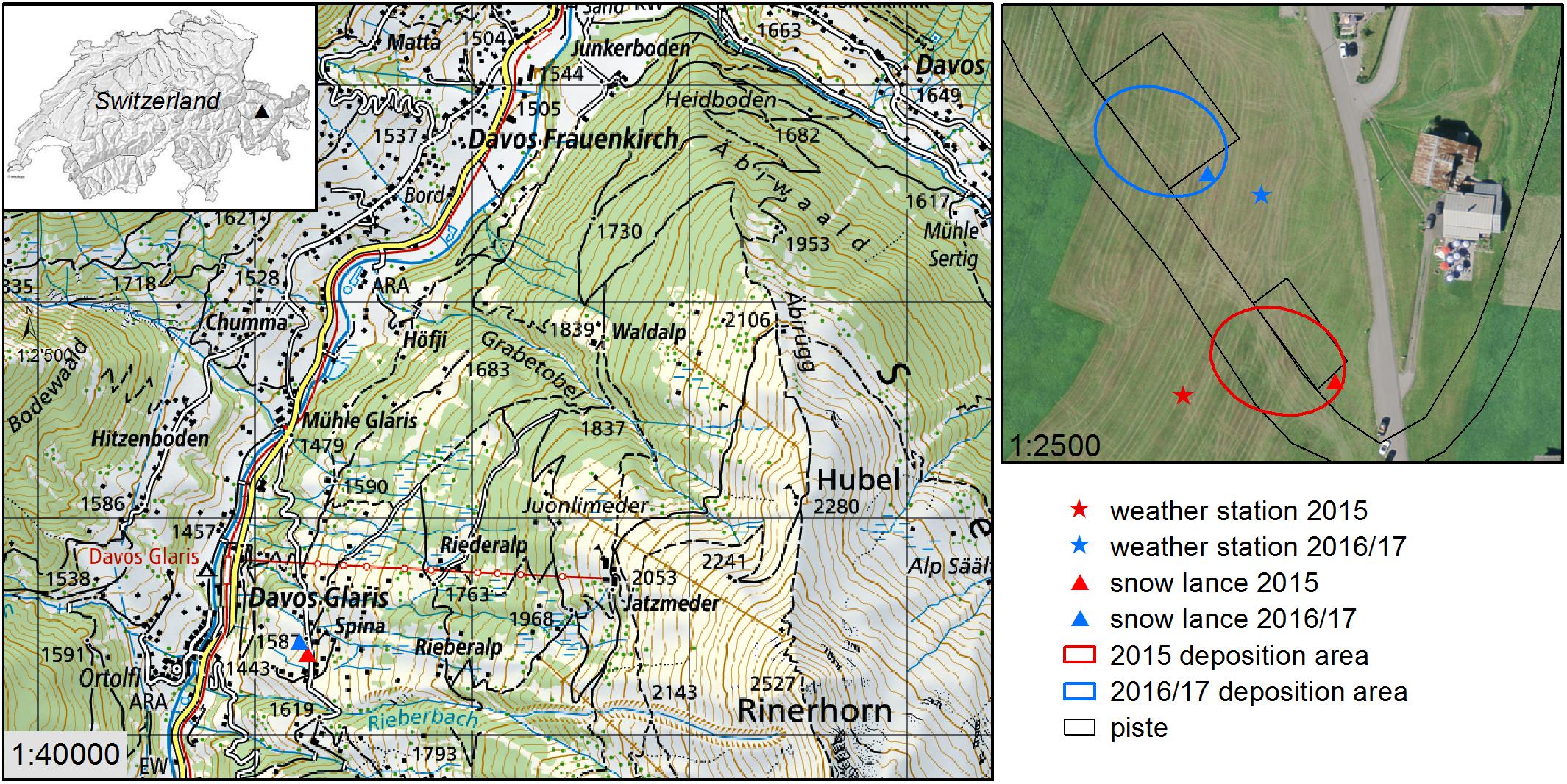
Figure 1. Topographic map and aerial photography of the study site at the Rinerhorn. Base maps: Swiss Map and swissimage© 2019 swisstopo (5704 000 000).
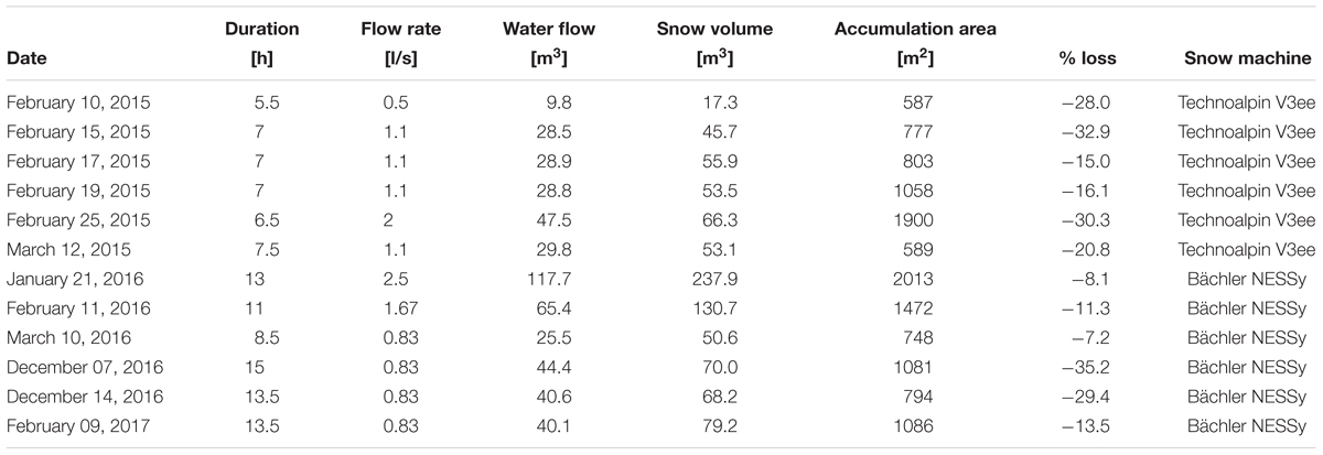
In the first year, a Technoalpin V3ee snow lance (red triangle in Figure 1) was used for six experiments (Table 1). Flow rates ranging from 0.5 to 2 l/s could be chosen for this snow machine. As the cumulated water flow was not captured automatically, we set a constant water flow for the entire night and manually documented operation time. Total water flow was cumulated from these settings.
In consecutive years, a Bächler NESSy snow lance was installed for another six experiments about 70 m downslope (Figures 1, 2 and Table 1). In comparison to the previous year, a larger undisturbed place adjacent to the ski run was available for the snow accumulation at this test site. Three flow rates could be selected: 0.83, 1.67, and 2.5 l/s. As in the first year, the lance ran with a constant flow rate for the entire duration of the experiment. Flow rate, water temperature, water pressure and, most important, cumulated water flow were automatically recorded with a separate flow meter mounted at the intake of the snow lance. Advantages of this new setup are the larger undistorted accumulation area and the direct record of the water inflow. Water required for snow production was withdrawn from the line system of the ski resort’s snow-making facilities and originated from an upstream ditch. Water temperatures were between 1 and 2°C.
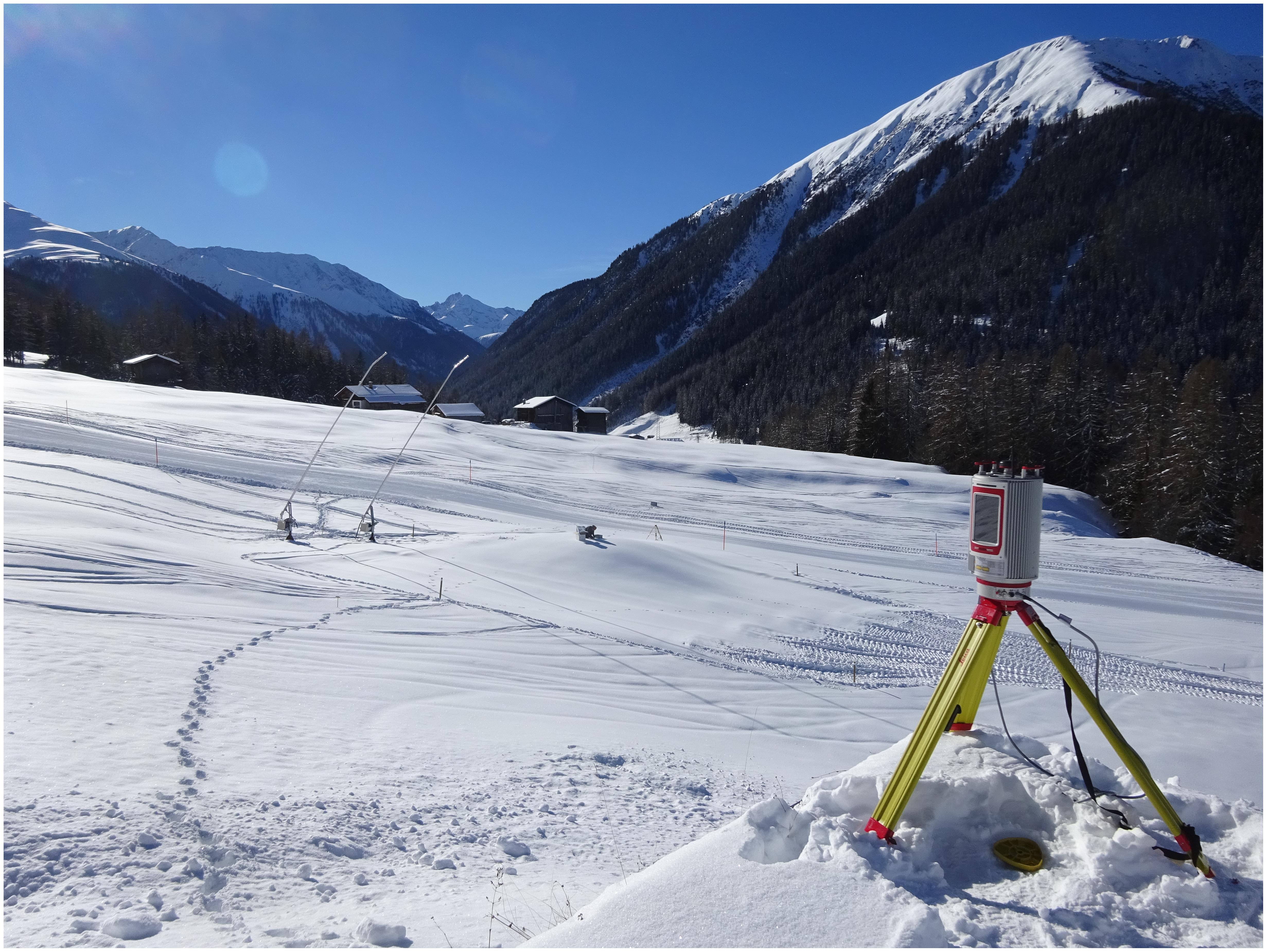
Figure 2. Study site at the Rinerhorn after snow-making experiment, seen from northeast. The Riegl VZ6000 is visible in the foreground.
Calculation of New Snow Height
Terrestrial laser scanning is a well-established method to acquire high resolution elevation models of snow surfaces with a vertical accuracy of some centimeters (Prokop et al., 2008; Grünewald et al., 2010, 2018b; Revuelto et al., 2014). The device deployed for this study was a Riegl VZ-6000 terrestrial laser scanner (Riegl Measurement Systems GmbH, 2018) that has been successfully applied to monitor snow surfaces and snow-height changes (dHSs) in several projects (e.g., Gabbud et al., 2015; Fischer et al., 2016; Haberkorn et al., 2017; Grünewald et al., 2018b; Mott et al., 2019). Technical specifications of the VZ6000 are listed by Fischer et al. (2016) and in the Riegl data sheet (Riegl Measurement Systems GmbH, 2018). One survey (February 10, 2015) was performed with a Riegl LPM321 (Riegl Measurement Systems GmbH, 2008; Grünewald et al., 2010). Properties, handling and performance of the LPM321 differ slightly from the VZ-6000 (wave length, accuracy, larger beam diameter) but appear insignificant due to the very small measurement distances. In this study angular step widths between 0.02 and 0.05°C were chosen, depending on the distance of the position of the scanner (30–80 m) to the snow heap. This results in raw point densities of several hundreds to thousands of points per square meter.
For each field experiment two TLS surveys were performed, one in the evening before snow-making started and a second one the next morning after setting off the snow machine. To avoid data gaps caused by terrain shadowing, scans were done from two to three positions. The workflow of post-processing was the same as described in Grünewald et al. (2018b). For each pair of surveys, raw data were registered with four reflectors installed in the area. Unchanged areas (without snow accumulation) were selected for Multi Station Adjustment, a semi-automatic least square surface matching technique implemented in the processing software (Riegl Measurement Systems GmbH, 2011). This technique was successfully applied by many studies for the registration of TLS data (Carrivick et al., 2013; Sommer et al., 2015; Fischer et al., 2016; Grünewald et al., 2018b). After selecting the area of interest, a moving-window filter (octree filter) was applied to reduce the data amount and to produce a regular grid with an edge length of 10 cm. A few larger data gaps (>1 m2) existed only for two of the scans (December 15, 2016 and February 10, 2017). Poor instrumental settings of the laser intensity in combination with the fresh, moist snow resulted in very low reflectivity at some sections of the snow pile. Mean point density was only a few points per square meter in these areas and point distances of up to 4 m were present. The gaps were closed by linear interpolation using ArcGIS 10.2 Delaunay triangulation with larger edge lengths (up to 5 m). Moreover, the morning survey from March 15, 2015 did not cover the full accumulation area – about 1/4 was missing. Area and mean snow height of this missing section were estimated based on the measured values and the geometry of the rest of the snow pile and then added to the measured snow volume.
Results are rasterized digital surface models with cell size of 10 cm. dHS and hence snow volume produced by the snow lance was then calculated by subtracting the two. Finally, outliers such as negative or extremely large dHS were filtered and replaced by mean values of the surrounding raster cells.
Snow Density
Snow densities (ρ) were collected manually for each field experiment by weighing samples of known volume. In the first year measurements were obtained with a 100 cm3 cubic density cutter (Proksch et al., 2016) near the snow surface. Along the main axis of the snow heap, four to five locations were sampled with three measurements each. From the second year on, 55 cm-long aluminum cylinders with a cross-sectional area of 70 cm2 were used instead (Jonas et al., 2009). This method appears more robust as sample volumes are larger and as bulk density of the entire fresh snow is gathered [if snow height (HS) > 55 cm, two samples were taken and merged afterward]. As this method appears more accurate but also time consuming, the number of samples was reduced (Table 2). Bulk density was now sampled at the point of the maximum snow accumulation and at up to two additional places about 2 m apart.
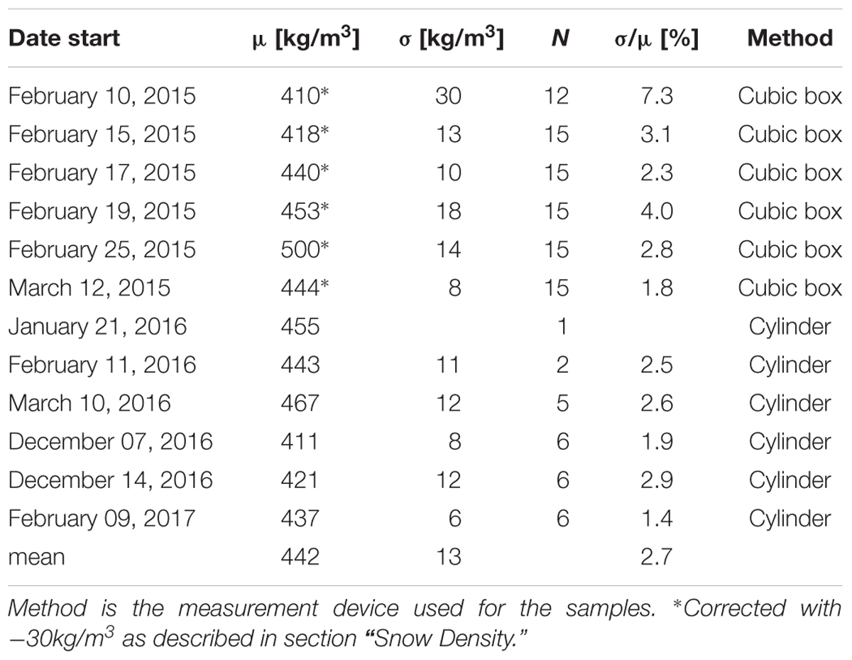
Table 2. Mean (μ), standard deviation (σ), number of observations (N), and relative uncertainty (σ/μ) of snow density [kg/m3] measured at the snow heaps.
Liquid Water Content (Snow Wetness)
Snow wetness is an important parameter frequently used to rate the quality of machine-made snow. The quality of technical snow is considered to decrease with increasing LWC as ski slopes tend to get icier and snow grains grow due to wet-snow metamorphism. This is disadvantageous for dry-snow sintering after tilling the frozen snow with snow groomers. Moreover, the proper functioning of a snow machine can be quantified by the LWC of the produced snow at a certain throughput in relation to atmospheric conditions. Based on the international classification of seasonal snow Fierz et al. (2009), Wolfsperger et al. (2018) suggested five classes to rate technical snow quality based on LWC: very high (dry snow), high (<3%), reasonable (3–8%), low (8–15%), and unsatisfactory (>15%). Concerning the investigation of water losses during snow-making, the LWC gives indications about possible losses by water drainage; water only starts percolating through the snow above volumetric contents of about 6% (Fierz et al., 2009).
Liquid water content can be calculated by measuring snow density and the dielectric constant of snow at a frequency of 20 MHz (Denoth, 1994). A prototype field measurement device developed by Denoth (1989) was applied with a 0.134 m × 0.129 m capacitive sensor resulting in a measurement volume of approximately 0.34572 ∗ 10-3 m3. The LWC was calculated from the measured dielectric constant (ε) and ρ by solving Denoth’s empirical parametrization function ε = f(ρ; LWC) for LWC (Denoth, 1989).
In the first year, three dielectric measurements were performed at each density sample point near to the snow surface. During the second winter LWC was not measured. To investigate vertical LWC differences, in the last winter, two measurements were performed in different depths at the point of the maximal snow height. The two to three epsilon and density values at each position or height were averaged, and LWC values were calculated with Eq. (1) and plotted over snow height or distance to snow lance. To check plausibility of LWC occurrence also snow temperatures were measured.
Calculation of Water Losses
To calculate relative water losses during technical snow production, the water inflow measured at the snow machine (see section “Study Site”) was related to the snow water equivalent (SWE) accumulated at the ground. For each experiment, the accumulation area (A) was visually identified (>1 mm of fresh snow) and mapped with a differential global navigation satellite system (dGNSS). In the few cases when no dGNSS device was available, accumulation areas were visually defined based on the TLS data (see section “Calculation of New Snow Height”). dHS rasters were then masked to this extent and cumulated to a total snow volume. Multiplying the mean snow-height change () with measured mean densities (ρ) adds up to a single amount of SWE as formulated in Eq. (2). Relating SWE to water inflow finally yields relative water losses.
Experimental Setup
The ideal experimental setup for a snow-making field experiment included the following steps: After the resort was closed in the afternoon, the test field and the adjacent ski run were leveled by a snow groomer. The smoothed field should be large enough to cover the entire accumulation area of the snow lance. Then, TLS measurements from the different scan positions were performed. Ideally, the entire area remained untouched from this point of time. As soon as temperatures were cold enough, water flow measurement and the snow lance were started with a flow rate balanced to the weather conditions. On the one hand, as the flow rate remained constant during the entire experiment, steady meteorological conditions should be present to receive snow of homogenous quality. On the other hand, long snow-making duration enhances amounts of snow produced and therefore limits impacts of potential measurement errors. Experiments were therefore started after sunset, when rather constant conditions were present and terminated before solar radiation started to heat the site and before ski runs were opened. Water flow records were read and TLS measurements performed immediately after the snow machine was set off. With the setup used here, TLS required less than 1 h for all three positions. About 15–30 min after switching the snow lance, dGNSS measurements of the accumulation area were performed and snow pits were dug to collect density and water content samples. The height of fresh snow that needed to be sampled for density and LWC measurements could easily be identified in the snow pit by its lower hardness due to its short time of sintering (growth of the grain bonds) from the time of its deposition on the ground.
The location in an operating ski resort, however, clearly limited this ideal setup in practice. It happened that the smoothed field was too small, such that some portions of the produced snow accumulated outside in the terrain, slightly reducing TLS accuracy (larger surface roughness, scan shadows). In other cases, snow groomers crossed the edge of the potential accumulation area after evening TLS measurements had been terminated. For the experiments performed in December 2016, bare ground or only small amounts of snow prohibited smoothing of the test field, leading to higher surface roughness. These impacts influenced data accuracy but are still small considering the high general accuracy of the measurements (relative snow volume error for rough surface 4% vs. mean relative snow volume error 3%, see section “New Snow Height and Snow Volume”).
Statistical Analysis
Statistical analysis (univariate linear and robust regression using the “stats” and “robustbase” packages in R) was applied to relate measured water losses during snow production to meteorological conditions (R Core Team, 2015; Maechler et al., 2016). The dependent variable is the relative water loss calculated from the measurements. Explanatory variables are recorded meteorological conditions TA, RH, VW, the standard deviation of VW [σ(VW)], and wet-bulb temperature (TWB). TWB was calculated from TA and RH by applying the parameterization of Stull (2011). Model performance was rated by R2 and adjusted R2 (R2adj) values, for model significance, p-values were checked. Finally, Quantile–Quantile plots and Tukey–Anscombe plots (Faraway, 2005) were examined to test for preconditions of linear regression (normal distribution and constant variance of residuals). It needs to be noted that the small number of observations (12) limits the statistical validity of the resulting models. Significance levels and model performance should therefore be interpreted carefully. Calculating models with multiple parameters (e.g., a combination of TA, RH, and VW) would be physically meaningful and interesting. However, as the small number of observations poses a high risk of overfitting, we do not show such models.
To enlarge the number of experiments, we complemented our data set with earlier measurements published by Eisel et al. (1988) and Spandre et al. (2017). Regression models with these combined data were then calculated. Eisel et al. (1988) provided mean values for TA, RH, and VW while TWB was calculated with the formula of Stull (2011). VWs characterized with “calm” were set to 0.1 m/s. Spandre et al. (2017) only released measured TWB and VW. TA and RH were not available.
Results and Discussion
Weather Conditions
Mean values and variability (expressed by standard deviation σ) of meteorological conditions measured at the weather station are listed in Table 3. As an example, Figure 3 shows measured values of wind, TA, RH and calculated TWB (Stull, 2011). TWB is the adiabatic saturation temperature. It describes the temperature to which a water droplet cools down until thermodynamic equilibrium with the surrounding air is reached. TWB is a meteorological parameter widely applied by the snow-making industry and practitioners. A TWB between -2°C and -4°C is the common range for the onset of snow-making (Olefs et al., 2010; Wolfsperger et al., 2018). The quantity of snow that can be produced is directly related to TWB: the lower the TWB, the more heat can be transferred from the water spray to the surrounding air, meaning that larger amounts of water can be frozen per time and therefore allow for higher water input and snow production rates. As the consumed electricity of a snow maker (energy for the ventilator and/or pressurized air) is constant, no matter how large the water throughput is, the efficiency of snow-making increases with colder TWB.
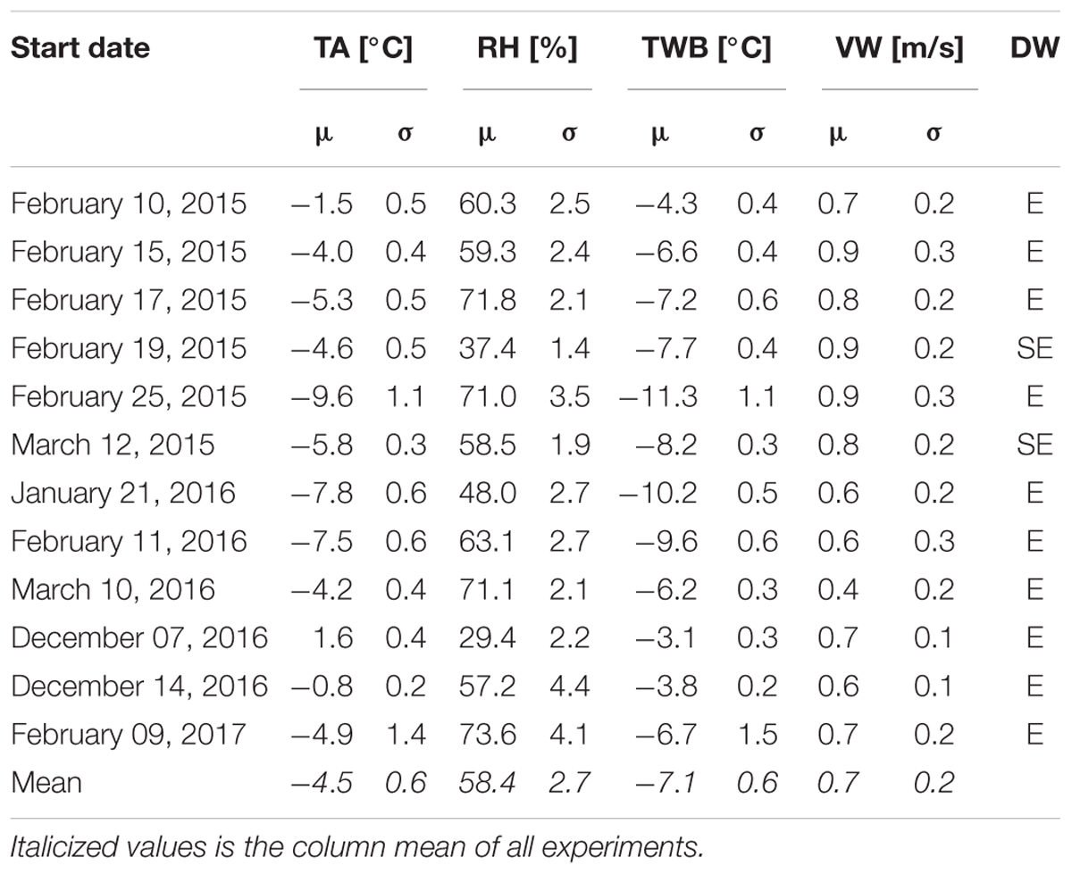
Table 3. Mean (μ) and standard deviation (σ) of measured air temperature (TA), relative humidity (RH), wind speed (VW), wind direction (DW), and calculated wet-bulb temperature (TWB).
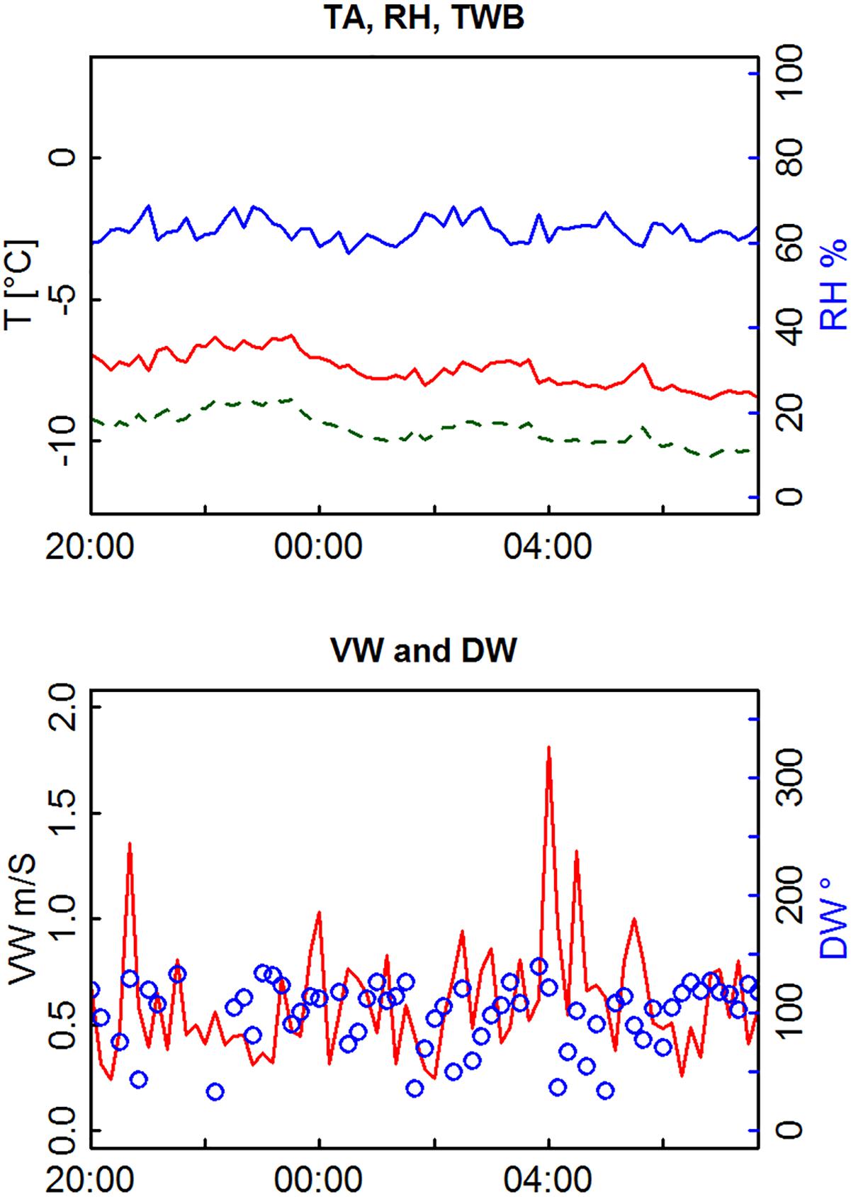
Figure 3. Meteorological measurements: air temperature (TA, red line upper panel), relative humidity (RH, blue line), wind speed (VW, red line lower panel), and wind direction (DW, blue circles) for experiment February 11/12, 2016. Wet-bulb temperature (TWB, green dashed line) was calculated from TA and RH (Stull, 2011). Hours are in local time.
For our experiments we aimed to picture a preferably wide range of meteorological conditions, best expressed by TWB. Mean TWB ranged from -3.1 to -11.3°C (mean = -7.1°C). The temporal variability during a night of snow-making was usually small (Table 3). Decreasing TA in the course of the night was mostly balanced by increasing RH, resulting in rather constant TWB. DWs were east to southeast and VWs were low, ranging from 0.4 to 0.9 m/s, and rather constant (σ = 0.1–0.3).
Snow Measurements
Snow Distribution and Volumes
Figure 4 shows heights of fresh snow produced during the experiment performed on February 11/12, 2016. Colors mark dHS obtained from the TLS surveys and the black line is the accumulation area monitored with dGNSS (HS > 1 mm). Note that the green colored areas in the southwest of the accumulation zone were caused by redistribution of snow by a groomer after the first laser scan had been performed.
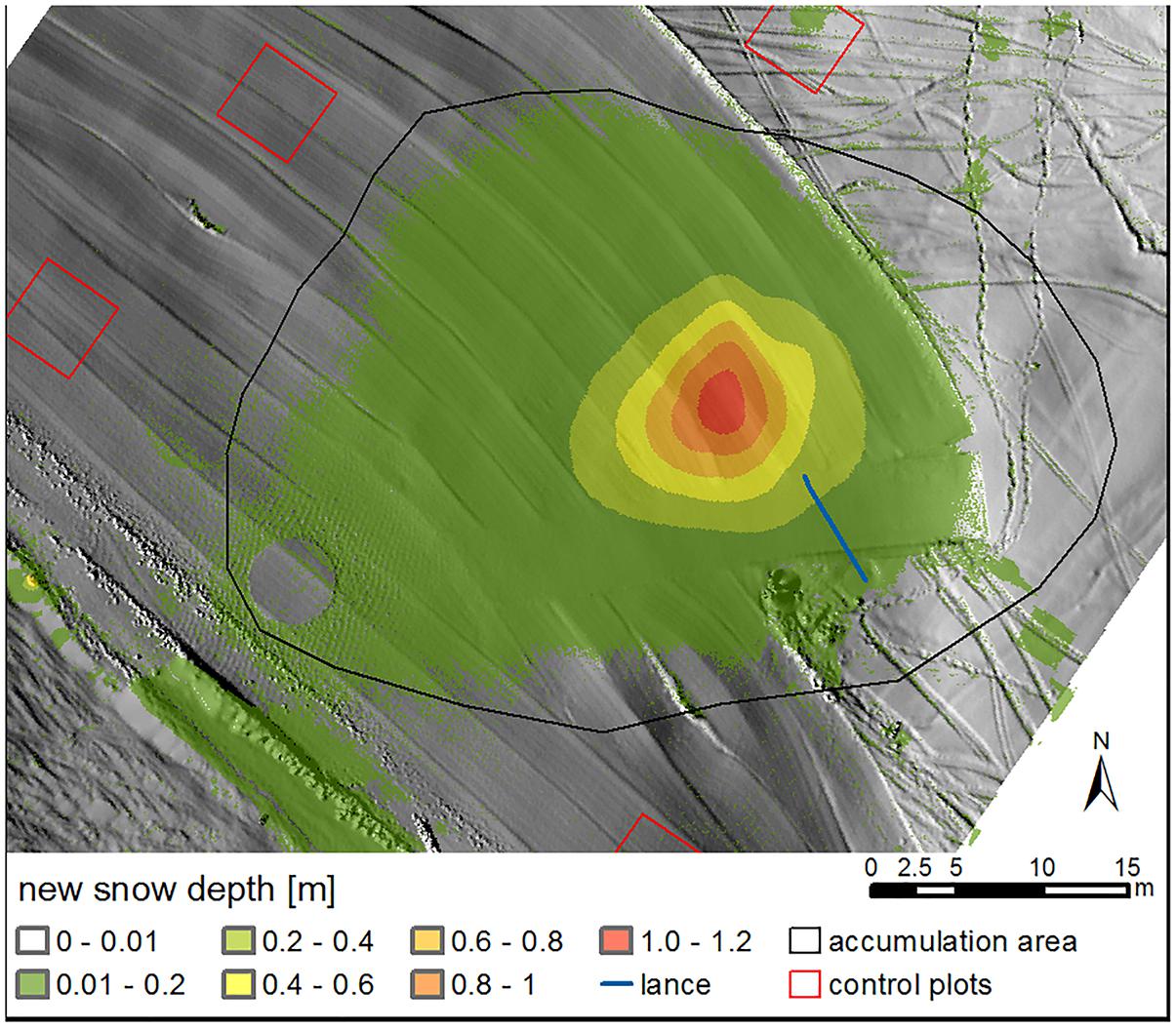
Figure 4. Height of the produced snow measured by terrestrial laser scanning for February 11/12, 2016. The black line marks the accumulation area deduced from dGNSS measurements of the visually recognized snow deposition. Red squares show examples for control plots.
The fresh snow covered an area of 1472 m2. Most of the snow was northwest of the snow lance which is consistent with the orientation of the lance and the direction of the wind. The peak of the snow pile, with a dHS of 1.2 m, was in a distance of about 6 m from the head (13.5 m from the foot) of the lance oriented to the same direction. Some snow, even though only small amounts, was also found in the back of the snow machine (Figure 4). Snow volume within the accumulation area was 131 m3.
Flow rate, snow height, snow volume, and accumulation area were higher at February 11/12 than the average of all experiments. In principal, these characteristics varied considerably depending on machine settings and atmospheric conditions (Table 1). The shape of the snow piles was, however, similar for all experiments.
Snow Density
As described in section “Snow Density,” two different devices were used to sample density. Both methods were applied simultaneously during the first experiment in 2016. Comparing the measurements of the two methods revealed clearly higher mean values and variability for the small cubic density cutter (cubic box). An overestimation of density by this method has also been reported by Proksch et al. (2016). On average these densities were 30 kg/m3 higher. This is probably attributed to additional compaction of the snow while cutting with the sample holder. For consistency between the experiments, we hence corrected all mean values obtained with the box method with a constant of –30 kg/m3.
Mean values and standard deviations of corrected snow densities are listed in Table 2. Daily averaged densities varied from 410 to 500 kg/m3. Heterogeneity between single samples, stated by σ, was also considerably expressing both natural variability and measurement uncertainty. The average of all experiments was 442 kg/m3 (σ = 13 kg/m3), which is similar to the 437 kg/m3 (σ = 18 kg/m3) published by Spandre et al. (2017). However, different to Spandre et al. (2017), we apply daily averages for each experiment instead of a constant overall mean.
Liquid Water Content
Liquid water content was measured at nine experiments. In three experiments no LWC was found. Nevertheless, the existence of a certain content of liquid water right after snow production can be assumed as the measured snow densities were higher than for dry technical snow (especially on February 25, 2015). The assumed liquid water had likely been frozen before LWC measurements were started 15 min after switching off the snow maker (see section “Experimental Setup”). In six experiments, wet snow was found with a maximum LWC ranging from 0.2 to 12.6%. Those maxima were always located at the position of maximal snow height (Figure 5). LWC above 6% was measured only on December 7 and 14, 2016, which indicates possible water drainage into deeper layers (base layers) of the snowpack.
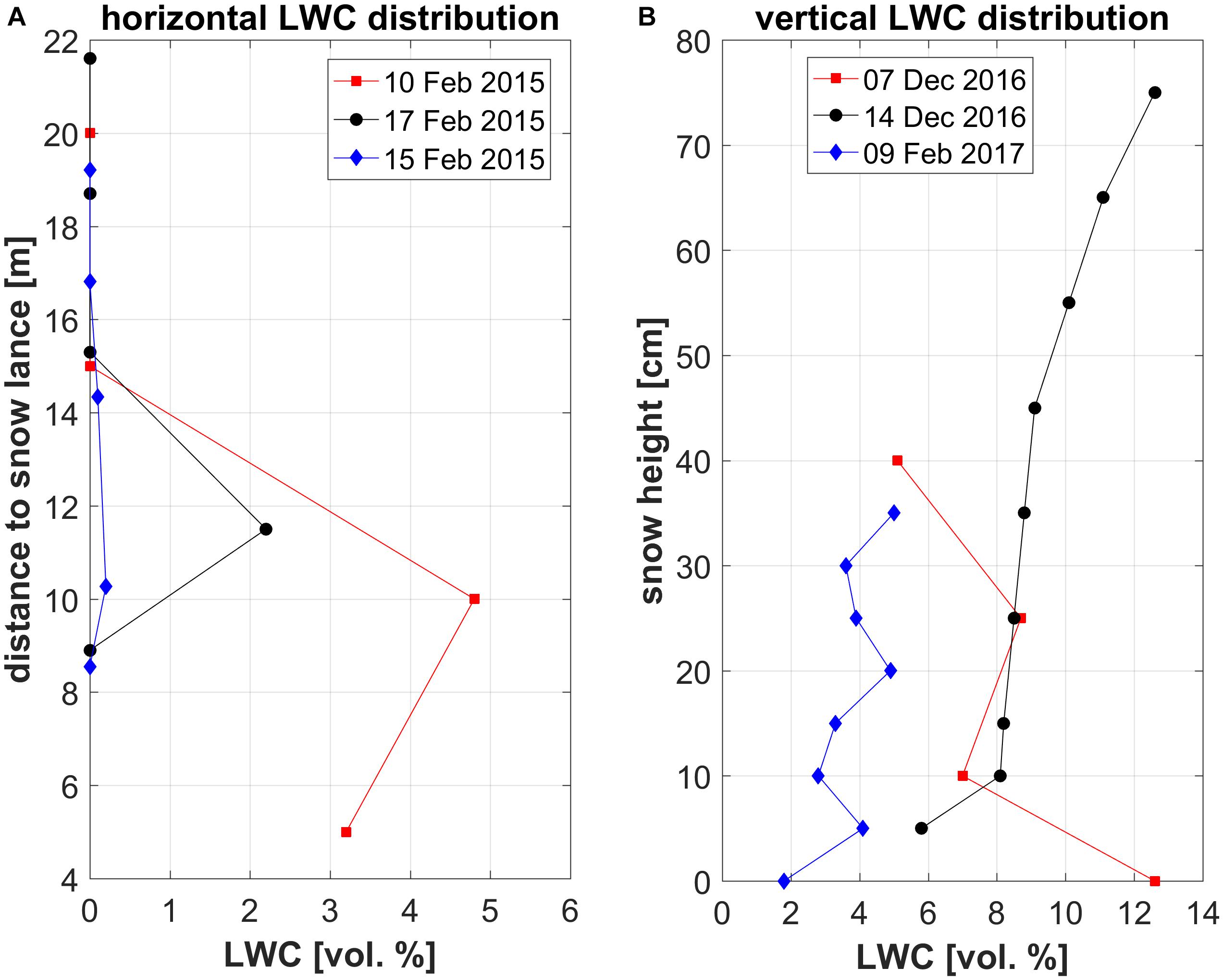
Figure 5. Examples for horizontal (A) and vertical (B) distributions of liquid water content (LWC) for six snow-making experiments.
Whereas the horizontal snow-wetness distribution showed similar patterns that were closely related to the distance to the snow lance as well as to the snow height distribution (Figure 5A), the vertical LWC distributions at the maximum snow height were more variable: On December 7 LWC increased from the snow surface to deeper layers. The other days the opposite was observed (Figure 5B). We consider the warmer TWB and the bare ground on which the snow was deposed as possible reasons for the differing LWC distribution on December 7. If snow is accumulated on frozen bare ground, water might accumulate at the bottom instead of percolating to deeper snow layers. Moreover, a snow layer acts as a better heat sink. It therefore considerably contributes to freezing of the free water in the produced snow. This is a result of the lower temperature of the snow and the cooling effect caused by the latent heat of melting of a quite large ice mass.
Water Losses
Measurements
Total water losses were calculated from SWE and measured water flow for each experiment as described in section “Calculation of Water Losses” and are summarized in Table 1. The mean of all experiments was 20.7% and the range was 7.2–35.2%.
Three physical processes come in consideration as sources of these water losses. These are (1) evaporation and sublimation of water droplets and ice particles while traveling through the air, (2) wind drift of particles and accumulation out of the bounds of the target area, and (3) drainage of unfrozen water on the ground. Distinguishing between these processes in an experimental setup is extremely challenging and hardly possible during operational conditions as presented here. Earlier studies estimated losses attributed to sublimation and evaporation between 2 and 13% (Eisel et al., 1988; Hanzer et al., 2014; Spandre et al., 2017). Losses caused by water draining on the ground were not considered in any of the mentioned studies. Nevertheless, we believe that this source of loss can be relevant, especially when snow with high initial water content is produced (as often done in ski resorts at warmer conditions or for base layer snow-making). The first four experiments described by Spandre et al. (2017) were characterized by high water input and we expect that the snow was rather wet. Outflow was not directly recorded but might well have happened (P. Spandre, personal communication June 8, 2017). Exactly those four experiments are the ones that revealed much higher water losses of 50%. Like Spandre et al. (2017), we do not have direct observations of draining water either. However, on December 7, 2016, when produced snow was accumulated on bare frozen ground, we could monitor a ca. 80 m2 ice plate that was frozen at the downslope edge of the snow heap. Assuming a thickness of about 2 cm and a density of 917 kg/m3 reveals 1.6 m3 of ice. This corresponds to 1.5 m3 of water or 5% of the water input. Ice plates were also visible during consecutive experiments, but it was not possible to distinguish between fresh ice and ice from the previous tests and the water amount could therefore not be quantified.
Finally, losses attributed to wind drift need to be considered. We only performed experiments during conditions with low VW. Hourly mean VW was below 1 m/s for all experiments (Table 2) and variability was also low (σ < 0.3 m/s). Even maximum VW of the raw measured data (resolution 10 min for 2015 and 2016 and 30 min for 2017) did not exceed 1.8 m/s. Still, our experiments showed that the maximum distance of the recorded snow accumulation to the lance varied considerably, ranging from 30 to 60 m. The large variability is also expressed by the size of the accumulation area (Table 1). An effect of the wind (Table 3) on the distribution of the produced snow is obvious. However, our data did not show a correlation between accumulation area and measured VW. From our measurements, we cannot directly quantify losses attributed to wind drift. Physically based models (see e.g., Mott et al., 2018) could possibly be applied to simulate deposition of snow during snow-making. Results could help to evaluate how much snow might be accumulated outside the measured area. In summary, it must be stated that our experiments were performed under conditions with low winds. In praxis, snow is frequently produced at higher VWs as are often present at higher and unsheltered locations. Under such conditions, larger accumulation areas must be expected.
Statistical Analysis
Scatter plots relating relative water losses to the meteorological quantities TA, RH, TWB, VW, and σ(VW) (Figure 6) indicate increasing water losses with increasing TA, TWB, and VW and a decrease with increasing RH. No trend can be identified for σ(VW). Statistical analysis applying ordinary least squares regression (OLS) does not result in statistically significant models: R2 between 0.2 and 0.3 and p-values > 0.1 would be detected for TA, TWB, VW, and RH.
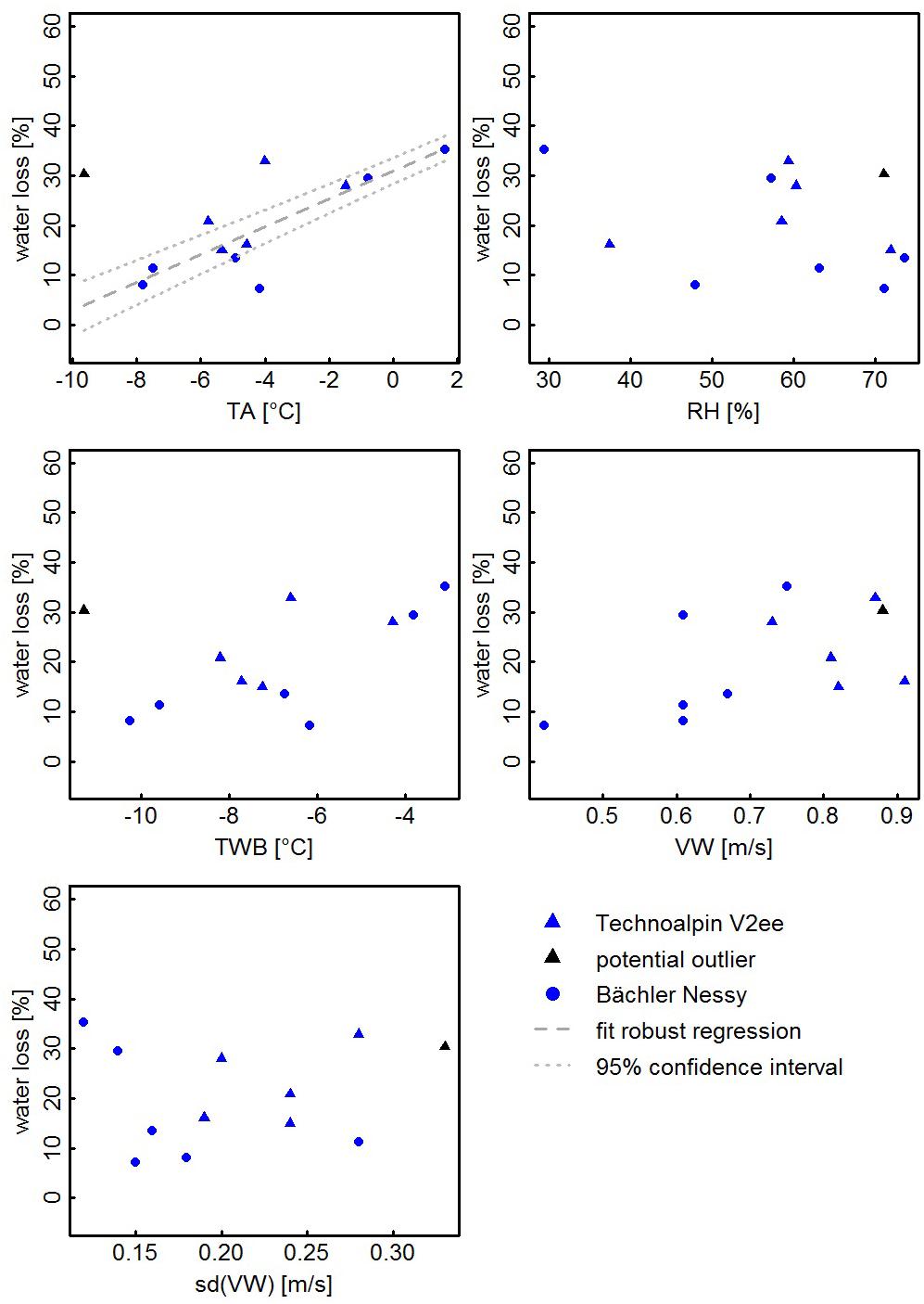
Figure 6. Scatterplots of calculated water losses vs. meteorological properties measured at the weather station. The potential outlier is the experiment of February 25, 2015.
A careful inspection of Figure 6 indicates that the water losses on February 25, 2015 deviate from the obvious correlation with TA and TWB. In relation to the cool temperatures at that day, the loss appears clearly too high. A possible explanation might be drainage of water to deeper snow layers. The flow rate was set higher than during earlier tests with this snow lance, and high snow densities and water content point at a possible loss of water due to outflow from the fresh snow. To test this hypothesis, we added water flow as a second explanatory variable. However, the regression models were not improved by that additional parameter. Moreover, the experiment performed on January 21, 2016 with similar conditions and settings revealed much lower water losses. From these findings, our hypothesis could therefore not be confirmed.
A second possible explanation is the wind. VWs, wind fluctuation, and accumulation area were among the largest of all experiments. An unknown quantity of snow might have been accumulated outside of the measured area and neglected for the volume measurements. Adding the wind as an additional parameter, we found a highly significant model (R2 = 0.7, p = 0.006) with TA and σ(VW) as explanatory variables (vs. R2 = 0.2, p = 0.1 for a model only with TA). Note that the model must be interpreted with caution due to the small number of observations. It can, however, serve as an indication that wind might be a valid explanation for the deviation of the February 25, 2015 observation. Removing this single observation results in a clear improvement of the regression models for TA (R2 = 0.6, p-value = 0.004) and TWB (R2 = 0.5, p-value = 0.01).
To test if any observation can be treated as an outlier in the statistical analysis, we calculated robust regression models with MM-type estimators (Yohai, 1987). A robust model with TA as the explanatory variable classifies the February 25 observation as an outlier and removes it from the model. The resulting model (Eq. (3), Figure 6) is highly significant (p-value < 0.001) and exhibits an R2 of 0.73 (R2Adj = 0.71).
R2 and the p-value given by the robust model need to be interpreted with care due to the small sample size and as they can be biased (Renaud and Victoria-Feser, 2010). The model (Eq. (3)) is, however, very similar to the OLS model after removing the February 25 observation. Robust models with the other parameters [TWB, VW, RH, and σ(VW)] were not statistically significant. Prerequisites for linear regression (normal distribution and constant variance of residuals) were tested. Analysis of Normal QQ plots and Tukey Anscombe plots (not shown) showed acceptable fulfillment of model assumptions.
In summary, the statistical analysis suggests that the largest portion of water losses can be explained by TA. This is attributed to increased sublimation and evaporation rates at warmer temperatures (e.g., Wever et al., 2009; Dai and Huang, 2014). This confirms the results of Eisel et al. (1988), who found an R2 of 0.64 for their experiments.
Figure 7 shows scatterplots of our data merged with measurements published by Eisel et al. (1988) and Spandre et al. (2017). The experiments by Eisel et al. (1988) nicely complement our measurements in terms of weather conditions. While our data set lacks field tests during very cold TAs, most of Eisel’s data were observed under such conditions. In contrast, the study of Eisel et al. (1988) has only two observations near to limiting temperature for snow-making (TWB between -2 and -4°C). Additionally, the data sets complement well for RH and TWB. Wind conditions are in a similar range. Trend lines with 95% confidence intervals for the statistically significant models with all combined data are also shown in Figure 7. Table 4 summarizes the statistics of each linear regression model and Eq. (4) shows the OLS model for the combination of our and Eisel’s measurements (R2 = 0.61, R2Adj = 0.59,p-value < 0.001).
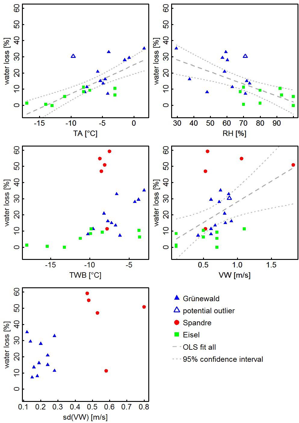
Figure 7. Same as Figure 6 but data set was merged with data from Eisel et al. (1988) and Spandre et al. (2017).
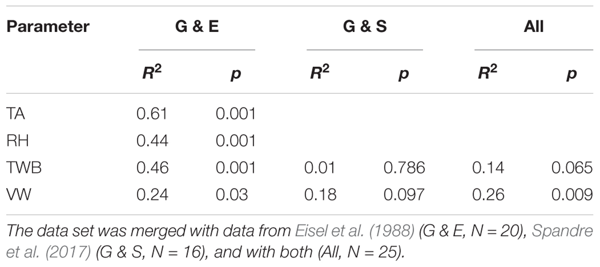
Table 4. Results of linear regression analysis with water loss (Y) as dependent variable and air temperature (TA), relative humidity (RH), wet-bulb temperature (TWB), and wind speed (VW) as explanatory variables.
The general trend of increasing water losses with increasing TA is similar to the robust model even though Eq. (4) differs from Eq. (3). Moreover, graphical impression indicates good agreement of our and Eisel’s measurements, also for TWB, RH, and VW (Figure 7).
In contrast, results obtained by Spandre et al. (2017) strongly differ (Figure 7). Water losses around 50% calculated from four experiments are clearly beyond the quantities that would be expected from our and Eisel’s data. Spandre et al. (2017) suggested that less than 10% of the losses could be explained by thermodynamic effects (sublimation and evaporation) and that the rest was attributed to “mechanical” effects such as the impact of wind and terrain. Wind, however, appeared not to be a satisfactory explanation as VWs were low and not higher than during the other experiments. It seems possible that unfrozen water drained on the ground during experiments as these field tests were performed with extremely high water input (P. Spandre, personal communication June 8, 2017). Still, this explanation appears insufficient to justify the tremendous quantity of the recorded water losses. Only the single experiment performed with reduced water flow and different machine settings revealed water losses that are well in line with our results. Consequently, the regression model with TWB including Spandre’s data (Figure 7 and Table 4) is characterized by reduced explanatory power and statistical significance. Residual analysis of the TWB model confirmed that the data of Spandre et al. (2017) do not fit this regression model. Only the model relating water losses to VW shows reasonable performance. The scatter in the data is high, though.
Data Accuracy and Precision
New Snow Height and Snow Volume
Accuracy of the TLS data was assessed by analyzing quadratic control plots. In total, 25 squares were placed at the undistorted ski run outside of the accumulation area of the snow lance as delineated in Figure 4. Each of the 25 m2 large plots contains 2500 cells. For each plot we calculated mean (μdHS) and standard deviation (σHS) of the two snow surfaces. Assuming that the surface of control plots did not change between the TLS surveys these result can be interpreted as a measure for accuracy of dHS and consequently also for snow volume. A mean bias of only 0.2 cm and a standard error (σHS) of 0.02 cm (RMS: 0.5 cm) prove the very high accuracy of TLS for short distances as applied here. The total error attributed to the dHs error (0.22 cm) on a mean deposition area of 1076 m2 would therefore result in a relative volume error of 3% (related to a mean snow heap volume of 77.4 m3).
Most of the produced snow accumulated on the groomed test site and ski run, but smaller portions were also found in open terrain or disturbed piste areas (see section “Experimental setup”). As expected, bias values (not shown) for such areas were larger but still clearly below 1 cm.
Moreover, some additional uncertainty might be introduced by the definition of the extent of the accumulation area. This was either done manually from the TLS data or mapped with dGNSS based on visual impression in the field. Extents could easily vary by some meters. If we consider the small HS at the edges of the area (few mm), the effect on snow volume is negligible.
Finally, data gaps in the TLS raw data caused by scan shadows (see section “Calculation of New Snow Height”) might induce some additional errors. As such gaps were very rare and – if present – quite small, their impact on total snow volumes can be neglected. Exceptions are the morning surveys on December 15, 2016 and February 10, 2017. Large data gaps (point spacing > 1 m) at the snow heaps had to be closed by interpolation. Such areas accumulated to be about 20 m2 for the first and to about 50 m2 for the latter survey. To quantify the potential volume error we assume a snow height deviation of 10 cm for these areas, resulting in 2 m3 (5 m3) of snow or 0.8 m3 (2.2 m3) of SWE. This corresponds to a portion of 2% (5%) of the water input of the respective experiments. Even higher is the error of the snow volume for March 12, 2016 when about 1/4 of the heap had not been surveyed in the morning due to technical problems. Area and volume of this area were estimated based on the geometric shape and the volume of the surveyed part of the heap. Assuming that this estimation incorporates an error of 10% results in an overall snow volume error of 2.5% (1/4 area ∗ 10% error).
Snow Density
As pictured in Table 2, snow density (ρ) comprises some variability, both spatially (at the same time but for different measurements) and temporally. This variability is on the one hand attributed to an inherent variance of the snow explained by its differing properties, such as grain size or LWC determined by the combination of weather conditions and machine settings (Wolfsperger et al., 2018). On the other hand a device-specific measurement error of some percent must be expected (Proksch et al., 2016).
The daily uncertainty related to density is expressed by its variation coefficient (σρ/μρ). A change in density linearly propagates to SWE (Eq. (1)). Increasing (decreasing) density by 1% will therefore increase (decrease) SWE and hence also water losses by the same portion. The relative uncertainties calculated for the daily density samples (Table 2) range from 1 to 7% with an average of 3%.
Water Flow
The water flow was controlled during the first year of experiments by the snow-making automation system of the ski resort. The water flow and the onset and offset times were set according to our wishes and water flow data were logged from the system every half hour. No information was available on the accuracy and precision of the water flow measurement. The following years a flowmeter turbine (FTB794-NB, Omega Engineering, Inc., United States) was used, which was over a 0–5 VDC output module (FLSC790-MA, Omega Engineering, Inc., United States) to an 8-bit field logger (CompactFieldPoint, cFP-2100, NI Inc., United States). The measurement system provided a measurement range of up to 6.33 l/s with a resolution of 0.025 l/s, which is lower than the flowmeters accuracy stated by the manufacturer (±1%). Deviations of the water flow linearly propagate to the error of the snow loss results, similar to density, and the snow volume errors.
Cumulative Error
To rate uncertainties of the final results, the single error terms described above need to be accumulated. Assuming linear error propagation allows adding up the single relative errors. This results in a maximal cumulative error of 7% (3% snow volume + 3% snow density + 1% water flow). Considering individual field tests, uncertainty is usually highest for experiments with low flow rates (due to warmer temperatures), resulting in less snow volume and therefore higher relative error. As shown before, these experiments are the ones revealing the highest water losses. Still, this rather high uncertainty underlines the tremendous importance of very careful execution and assessment of each component of the measurement setup.
Conclusion and Outlook
We presented measurements of 12 field experiments performed to quantify water losses during technical snow production near Davos, Switzerland. Weather conditions were variable, with mean wet-bulb temperatures ranging from -3.1 to -11.3°C. VWs were always low during the experiments. Snow volumes calculated from repeated TLS and density measurements were compared to measured water input at the snow machine. Water losses ranged from 7 to 35 (±7) % of the initial water input. Scatter plots show that the loss increased with TA, TWB and VW and decreased with RH. Robust regression revealed an R2 of 0.73 for TA whereas regression models with the other explanatory parameters TWB, RH, VW, and σ(VW) were much poorer and statistically not significant. Combining our results with data from an earlier study (Eisel et al., 1988) confirmed the relation between TA and water loss.
Still, the number of experimental observations on technical snow-making is very limited. Additional measurements are therefore required to add to the data basis. A larger data set could be used to formulate transferable and robust interrelations between water losses, weather conditions, and machine settings. This would enhance our understanding of snow-making and could be used to advance snow-making implementations in snow management models (e.g., Hanzer et al., 2014; Spandre et al., 2017) and finally to improve operational snow management. Fortunately, a rising number of ski resorts, public agencies, and snow industry players are currently detecting the demand for systematic field tests. In that context, the “Schneezentrum Tirol” (Schneezentrum, 2018) is currently developing a new, well-equipped test site that will soon start with systematic snow-making experiments (Grünewald et al., 2018a). Another attempt aiming to improve snow-making technology is the Norwegian “Snow for the future” project (SINTEF, 2018).
Our experimental setup did not allow distinguishing between potential sources of loss, which are sublimation and evaporation of water droplets and ice grains, relocation of particle by wind and drainage of liquid water on the ground. Experimental setups to separate these processes are challenging but not impossible. For example, water drainage could be detected by a buried lysimeter as described by Würzer et al. (2017). Additionally, indoor snow-making facilities could be an environment to exclude snow drift effects (Clulow, 2006). Physical models could also possibly help to overcome these shortcomings. For example, large eddy simulation (LES) models could be used to simulate accumulation areas under variable wind conditions, and high resolution snowpack models (e.g., Lehning et al., 2002; Wever et al., 2015) could be applied to assess quantity and timing of water draining though a wet pile of machine-made snow. Finally, numerical models of drifting snow that account for thermodynamic effects of sublimating snow particles while traveling through the air (e.g., Thorpe and Mason, 1966; Dery et al., 1998; Wever et al., 2009; Groot Zwaaftink et al., 2013; Sharma et al., 2018) could be adapted to model physical processes during snow-making. Such physical processes involved, their implications, dimensions, and interdependencies could be systematically analyzed. This could, for example, help to quantity transfers of heat and mass during different ambient conditions and machine settings. Open questions such as those on the amounts of water lost by sublimation and evaporation and on the quantity of the respective cooling effect and therefore the contribution to freezing of the droplets during snow-making could possibly be answered.
Author Contributions
TG is the main author of this study, the main conductor of study design, fieldwork, data analysis, data interpretation, and manuscript preparation. FW significantly contributed in all mentioned parts of this publication.
Funding
Parts of this study were conducted within the framework of the Swiss Competence Center for Energy Research – Supply of Electricity (SCCER-SoE) with funding from the Commission for Technology and Innovation CTI (Grant No. 2013.0288). Moreover, this project was partly funded by the European Union’s Horizon 2020 Research and Innovation Program (PROSNOW Grant Agreement No. 730203).
Conflict of Interest Statement
The authors declare that the research was conducted in the absence of any commercial or financial relationships that could be construed as a potential conflict of interest.
Acknowledgments
We want to acknowledge all people who contributed to the successful completion of this manuscript. We thank Nigg Conrad and his team (Rinerhorn cable cars) for provision of infrastructure and their great support during field experiments. For support in fieldwork we are grateful to our colleges, namely Fabian Hegar, Christian Simeon, and Silvan Castelmur. We also thank Michael Lehning and Hansueli Rhyner for their support and valuable input. Finally, we acknowledge the reviewers, DS, MF, US, the editor TB and the editorial office for their valuable comments and suggestions.
References
Bintanja, R. (2001). Snowdrift sublimation in a katabatic wind region of the Antarctic ice sheet. J. Appl. Meteorol. 40, 1952–1966. doi: 10.1175/1520-0450(2001)040<1952:SSIAKW>2.0.CO;2
Carrivick, J. L., Geilhausen, M., Warburton, J., Dickson, N. E., Carver, S. J., Evans, A. J., et al. (2013). Contemporary geomorphological activity throughout the proglacial area of an alpine catchment. Geomorphology 188, 83–95. doi: 10.1016/j.geomorph.2012.03.029
Dai, X. Q., and Huang, N. (2014). Numerical simulation of drifting snow sublimation in the saltation layer. Sci. Rep. 4:6611. doi: 10.1038/srep06611
Dawson, J., and Scott, D. (2013). Managing for climate change in the alpine ski sector. Tour. Manag. 35, 244–254. doi: 10.1016/j.tourman.2012.07.009
Denoth, A. (1989). Snow dielectric measurements. Adv. Space Res. 9, 233–243. doi: 10.1016/0273-1177(89)90491-90492
Denoth, A. (1994). An electronic device for long-term snow wetness recording. Ann. Glaciol. 19, 104–106. doi: 10.1017/S0260305500011058
Dery, S. J., Taylor, P. A., and Xiao, J. B. (1998). The thermodynamic effects of sublimating, blowing snow in the atmospheric boundary layer. Bound. Layer Meteorol. 89, 251–283. doi: 10.1023/a:1001712111718
Dery, S. J., and Yau, M. K. (1999). A climatology of adverse winter-type weather events. J. Geophys. Res. Atmos. 104, 16657–16672. doi: 10.1029/1999jd900158
Eisel, L. M., Mills, K. D., and Leaf, C. F. (1988). Estimated consumptive loss from man-made snow. J. Am. Water Res. Assoc. 24, 815–820. doi: 10.1111/j.1752-1688.1988.tb00932.x
Falk, M. (2013). A survival analysis of ski lift companies. Tour. Manag. 36, 377–390. doi: 10.1016/j.tourman.2012.10.005
Fierz, C., Armstrong, R. L., Durand, Y., Etchevers, P., Greene, E., McClung, D. M., et al. (2009). The International Classification for Seasonal Snow on the Ground. Paris: UNESCO-IHP.
Fischer, M., Huss, M., Kummert, M., and Hoelzle, M. (2016). Application and validation of long-range terrestrial laser scanning to monitor the mass balance of very small glaciers in the Swiss Alps. Cryosphere 10, 1279–1295. doi: 10.5194/tc-10-1279-2016
Gabbud, C., Micheletti, N., and Lane, S. N. (2015). Lidar measurement of surface melt for a temperate Alpine glacier at the seasonal and hourly scales. J. Glaciol. 61, 963–974. doi: 10.3189/2015JoG14J226
Groot Zwaaftink, C. D., Löwe, H., Mott, R., Bavay, M., and Lehning, M. (2011). Drifting snow sublimation: a high resolution 3-D model with temperature and moisture feedbacks. J. Geophys. Res. 116:D16107. doi: 10.1029/2011JD01
Groot Zwaaftink, C. D., Mott, R., and Lehning, M. (2013). Seasonal simulation of drifting snow sublimation in Alpine terrain. Water Res. Res. 49, 1581–1590. doi: 10.1002/wrcr.20137
Grünewald, T., Rothleitner, M., and Pupp, M. (2018a). “A new test site to investigate machine-made snow production,” in the Proceedings of the International Snow Science Work Shop ISSW, Innsbruck, WA.
Grünewald, T., Wolfsperger, F., and Lehning, M. (2018b). Snow farming: conserving snow over the summer season. Cryosphere 12, 385–400. doi: 10.5194/tc-12-385-2018
Grünewald, T., Schirmer, M., Mott, R., and Lehning, M. (2010). Spatial and temporal variability of snow depth and ablation rates in a small mountain catchment. Cryosphere 4, 215–225. doi: 10.5194/tc-4-215-2010
Haberkorn, A., Wever, N., Hoelzle, M., Phillips, M., Kenner, R., Bavay, M., et al. (2017). Distributed snow and rock temperature modelling in steep rock walls using Alpine3D. Cryosphere 11, 585–607. doi: 10.5194/tc-11-585-2017
Hanzer, F., Marke, T., and Strasser, U. (2014). Distributed, explicit modeling of technical snow production for a ski area in the Schladming region (Austrian Alps). Cold Reg. Sci. Technol. 108, 113–124. doi: 10.1016/j.coldregions.2014.08.003
Jonas, T., Marty, C., and Magnusson, J. (2009). Estimating the snow water equivalent from snow depth measurements in the swiss alps. J. Hydrol. 378, 161–167. doi: 10.1016/j.jhydrol.2009.09.021
Lehning, M., Bartelt, P. B., Brown, R. L., Fierz, C., and Satyawali, P. (2002). A physical SNOWPACK model for the swiss avalanche warning services. Part II: snow microstructure. Cold Reg. Sci. Technol. 35/ 3, 147–167. doi: 10.1016/S0165-232x(02)00073-73
Liston, G. E., and Sturm, M. (1998). A snow-transport model for complex terrain. J. Glaciol. 44, 498–516. doi: 10.3189/S0022143000002021
Maechler, M., Rousseeuw, P., Croux, C., Todorov, V., Ruckstuhl, A., Salibian-Barrera, M., et al. (2016). robustbase: Basic Robust Statistics R Package Version 0.92–97.
Mott, R., Vionnet, V., and Grünewald, T. (2018). The seasonal snow cover dynamics: review on wind-driven coupling processes. Front. Earth Sci. 6:197. doi: 10.3389/feart.2018.00197
Mott, R., Wolf, A., Kehl, M., Kunstmann, H., Warscher, M., and Grünewald, T. (2019). Avalanches and micrometeorology driving mass and energy balance of the lowest perennial ice field of the Alps: a case study. Cryosph. Discuss. (in press). doi: 10.5194/tc-2018-2255
Neumann, T. A., Albert, M. R., Engel, C., Courville, Z., and Perron, F. (2009). Sublimation rate and the mass-transfer coefficient for snow sublimation. Int. J. Heat Mass Transfer 52, 309–315. doi: 10.1016/j.ijheatmasstransfer.2008.06.003
Neumann, T. A., Albert, M. R., Lomonaco, R., Engel, C., Courville, Z., and Perron, F. (2008). Experimental determination of snow sublimation rate and stable-isotopic exchange. Ann. Glaciol. 49, 1–6. doi: 10.3189/172756408787814825
Olefs, M., Fischer, A., and Lang, J. (2010). Boundary conditions for artificial snow production in the Austrian alps. J. Appl. Meteorol. Climatol. 49, 1096–1113. doi: 10.1175/2010jamc2251.1
Prokop, A., Schirmer, M., Rub, M., Lehning, M., and Stocker, M. (2008). A comparison of measurement methods: terrestrial laser scanning, tachymetry and snow probing, for the determination of spatial snow depth distribution on slopes. Ann. Glaciol. 49, 210–216. doi: 10.3189/172756408787814726
Proksch, M., Rutter, N., Fierz, C., and Schneebeli, M. (2016). Intercomparison of snow density measurements: bias, precision, and vertical resolution. Cryosphere 10, 371–384. doi: 10.5194/tc-10-371-2016
R Core Team (2015). R: A Language and Environment for Statistical Computing. Vienna: R Foundation for Statistical Computing.
Renaud, O., and Victoria-Feser, M.-P. (2010). A robust coefficient of determination for regression. J. Stat. Plan. Inference 140, 1852–1862. doi: 10.1016/j.jspi.2010.01.008
Revuelto, J., López-Moreno, J. I., Azorin-Molina, C., Zabalza, J., Arguedas, G., and Vicente-Serrano, S. M. (2014). Mapping the annual evolution of snow depth in a small catchment in the Pyrenees using the long-range terrestrial laser scanning. J. Maps 10, 379–393. doi: 10.1080/17445647.2013.869268
Riegl Measurement Systems GmbH (2008). Long-Range Laser Profile Measuring System LPM-321. Technical Documentation and Operating Instructions. Version 04/07 CE. Horn: Riegl Measurement Systems GmbH .
Riegl Measurement Systems GmbH (2011): RiScan Pro: Viewer, Acquisition and Processing Software, Technical Documentation and Users Instructions. Horn: Riegl Measurement Systems GmbH.
Riegl Measurement Systems GmbH (2018). Data Sheet RIEGL VZ-6000. Available at: http://www.riegl.com/uploads/tx_pxpriegldownloads/RIEGL_VZ-6000_Datasheet_2018-12-05.pdf (accessed April 4, 2019).
Rixen, C., Teich, M., Lardelli, C., Gallati, D., Pohl, M., Pütz, M., et al. (2011). Winter tourism and climate change in the alps: an assessment of resource consumption, snow reliability, and future snowmaking potential. Mount. Res. Dev. 31, 229–236. doi: 10.1659/mrd-journal-d-10-00112.1
Schmidt, R. A. (1982). Vertical profiles of wind speed, snow concentration, and humidity in blowing snow. Bound. Layer Meteorol. 23, 223–246. doi: 10.1007/bf00123299
Schneezentrum. (2018). Schneezentrum Tirol. Available at: http://www.lebensraum.tirol/schneezentrum-tirol/ (accessed December 4, 2018).
Scott, D., and McBoyle, G. (2007). Climate change adaptation in the ski industry. Mitig. Adapt. Strateg. Global Change 12, 1411–1431. doi: 10.1007/s11027-006-9071-9074
Sharma, V., Comola, F., and Lehning, M. (2018). On the suitability of the thorpe-mason model for calculating sublimation of saltating snow. Cryosph. Discuss. 2018, 1–13. doi: 10.5194/tc-2018-2033
SINTEF (2018). Snow for the Future. Available at: https://www.sintef.no/en/projects/snow-for-the-future-will-produce-artificial-snow-s/ (accessed December 4, 2018).
Sommer, C. G., Lehning, M., and Mott, R. (2015). Snow in a very steep rock face: accumulation and redistribution during and after a snowfall event. Front. Earth Sci. 3:73. doi: 10.3389/feart.2015.00073
Spandre, P., François, H., Thibert, E., Morin, S., and George-Marcelpoil, E. (2017). Determination of snowmaking efficiency on a ski slope from observations and modelling of snowmaking events and seasonal snow accumulation. Cryosphere 11, 891–909. doi: 10.5194/tc-11-891-2017
Spandre, P., Morin, S., Lafaysse, M., Lejeune, Y., François, H., and George-Marcelpoil, E. (2016). Integration of snow management processes into a detailed snowpack model. Cold Regions Sci. Technol. 125, 48–64. doi: 10.1016/j.coldregions.2016.01.002
Steiger, R., and Mayer, M. (2008). Snowmaking and climate change future options for snow production in tyrolean ski resorts. Mount. Res. Dev. 28, 292–298. doi: 10.1659/mrd.0978
Steiger, R., Scott, D., Abegg, B., Pons, M., and Aall, C. (2017). A critical review of climate change risk for ski tourism. Curr. Issues Tour. 1–37. doi: 10.1080/13683500.2017.1410110
Stull, R. (2011). Wet-bulb temperature from relative humidity and air temperature. J. Appl. Meteorol. Climatol. 50, 2267–2269. doi: 10.1175/jamc-d-11-0143.1
Thorpe, A. D., and Mason, B. J. (1966). The evaporation of ice spheres and ice crystals. Brit. J. Appl. Phys. 17, 541–548. doi: 10.1088/0508-3443/17/4/316
Vanham, D., Fleischhacker, E., and Rauch, W. (2008). Technical note: seasonality in alpine water resources management – a regional assessment. Hydrol. Earth Syst. Sci. 12, 91–100. doi: 10.5194/hess-12-91-2008
Wever, N., Lehning, M., Clifton, A., Ruedi, J. D., Nishimura, K., Nemoto, M., et al. (2009). Verification of moisture budgets during drifting snow conditions in a cold wind tunnel. Water Res. Res. 45:14. doi: 10.1029/2008wr007522
Wever, N., Schmid, L., Heilig, A., Eisen, O., Fierz, C., and Lehning, M. (2015). Verification of the multi-layer SNOWPACK model with different water transport schemes. Cryosphere 9, 2271–2293. doi: 10.5194/tc-9-2271-2015
Wolfsegger, C., Gössling, S., and Scott, D. (2008). Climate change risk appraisal in the austrian ski industry. Tour. Rev. Int. 12, 13–23. doi: 10.3727/154427208785899948
Wolfsperger, F., Rhyner, H. U., and Schneebeli, M. (2018). Pistenpräparation und Pistenpflege. Das Handbuch für den Praktiker. Davos, CH: WSL-Insitut für Schnee- und Lawinenforschung SLF.
Würzer, S., Wever, N., Juras, R., Lehning, M., and Jonas, T. (2017). Modelling liquid water transport in snow under rain-on-snow conditions - considering preferential flow. Hydrol. Earth Syst. Sci. 21, 1741–1756. doi: 10.5194/hess-21-1741-2017
Keywords: snow-making, machine-made snow, water loss, technical snow, winter tourism, meteorological conditions, linear regression, terrestrial laser scanning
Citation: Grünewald T and Wolfsperger F (2019) Water Losses During Technical Snow Production: Results From Field Experiments. Front. Earth Sci. 7:78. doi: 10.3389/feart.2019.00078
Received: 06 November 2018; Accepted: 26 March 2019;
Published: 16 April 2019.
Edited by:
Timothy C. Bartholomaus, University of Idaho, United StatesReviewed by:
Daniel Scott, University of Waterloo, CanadaMartin Falk, Austrian Institute of Economic Research, Austria
Ulrich Strasser, University of Innsbruck, Austria
Copyright © 2019 Grünewald and Wolfsperger. This is an open-access article distributed under the terms of the Creative Commons Attribution License (CC BY). The use, distribution or reproduction in other forums is permitted, provided the original author(s) and the copyright owner(s) are credited and that the original publication in this journal is cited, in accordance with accepted academic practice. No use, distribution or reproduction is permitted which does not comply with these terms.
*Correspondence: Thomas Grünewald, Z3J1ZW5ld2FsZEBzbGYuY2g=
 Thomas Grünewald
 Fabian Wolfsperger