 Stefano Pollastri
 Eduardo Rossi
 Costanza Bonadonna
 Jonathan P. Merrison2
- 1Department of Earth Sciences, University of Geneva, Geneva, Switzerland
- 2Department of Physics and Astronomy, Aarhus University, Aarhus, Denmark
The fine ash released into the atmosphere (particles <63 μm) during explosive volcanic eruptions represents a significant threat for both the ecosystem and many sectors of society. In order to mitigate the associated impact, ash dispersal models need to accurately estimate ash concentration through time and space. Since most fine ash sediments in the form of aggregates, ash dispersal models require a quantitative description of ash aggregation. The physical and chemical processes involved in the collision and sticking of volcanic ash have been extensively studied in the last few decades. Among the different factors affecting volcanic particle aggregation (e.g., turbulence, particle-particle adhesion, presence of liquid and solid water), the charge carried by volcanic particles has been found to play a crucial role. However, Coulomb interactions are not yet taken into account in existing models. In order to fill this gap, we propose a strategy to take charge into account. In particular, we introduce a quantitative model for aggregation of oppositely charged micron—to millimetre-sized objects settling in still air. Our results show that the presence of charge considerably enhances the collision efficiency when one of the colliding objects is very small (<20 µm), and that the sticking efficiency is not affected by particle charge if colliding objects are either small enough (<20 µm) or large enough (>200 µm). Besides providing a theoretical framework to quantify the effect of charge, our findings demonstrate that aggregation models that do not account for electrification significantly underestimate the amount of fine ash that sediments in the form of aggregates, leading to an overestimation of the residence time of fine ash in the atmosphere after explosive volcanic eruptions.
Introduction
Volcanic explosive eruptions are typically associated with the injection of a large amount of fine ash (particles <63 µm) into the atmosphere (Rose and Durant (2009)). Recent eruptions have demonstrated the potential threat of volcanic ash on various transport systems (e.g. road network, aviation) as well as agriculture and public health (e.g. 2010 Eyjafjallajökull eruption, Iceland; 2011 Cordon Caulle eruption, Chile; 2020 Taal eruption, Philippines; Lund and Benediktsson (2011); Elissondo et al. (2016). In order to mitigate the associated risk, atmospheric ash concentration as well as ground mass loading over time and space need to be accurately described. It is important to notice that volcanic ash does not settle as individual particles but is largely affected by size-selective sedimentation processes that include particle aggregation and gravitational instabilities (e.g. Durant (2015)). In particular, extensive field observations show that during explosive eruptions most of fine ash sediments in the form of aggregates of various types (Taddeucci et al. (2011); Brown et al. (2012); Bagheri et al., 2016). Therefore, a quantitative understanding of aggregation processes is necessary to numerically describe and forecast ash dispersal and sedimentation (e.g. Costa et al. (2010)). Such a quantitative understanding requires the identification and quantification of fundamental parameters that control particle aggregation (e.g. collision velocity, particle mass, particle charge, amount of liquid or solid water on particle surfaces). Among these parameters, charge plays a fundamental role. Volcanic particles are seen to acquire electric charges during magma fragmentation and ejection from the vent (James et al. (2000); Mather and Harrison (2006); Méndez and Dufek (2016)). The spectacular phenomenon of lightning that often takes place during explosive eruptions is the visible proof that electrical potential gradients are present within volcanic plumes (e.g. Cimarelli et al. (2014); James et al. (2008); Cimarelli et al. (2016); Aizawa et al. (2016); Nicoll et al. (2019); Behnke et al. (2018)). The variation of these gradients during ash fall is evidence that volcanic particles are electrically charged. Particle charge can be indirectly estimated by measuring the variation of potential gradients (Hatakeyama (1943); Hatakeyama (1947); Hatakeyama (1949); Hatakeyama and Uchikawa (1951); Hatakeyama (1958)). The first direct measurements of charge carried by settling volcanic particles was performed by Gilbert et al. (1991) at Sakurajima volcano (Japan). Letting volcanic particles fall through the plates of a high voltage condenser, Gilbert et al. (1991) observed that volcanic particles could carry either positive or negative charges the value of which could be close to the ionization limit. They proposed that this charge might arise due to two mechanisms: triboelectric charging and fracture-induced electrification. In particular, the importance of the latter mechanism was stressed during magma fragmentation, suggesting that volcanic particles could preserve a significant charge since their formation. The effectiveness of the fracture-charging mechanism has been experimentally confirmed by James et al. (2000), who measured the charge generated during pumice fracture, obtaining charges of the same order of magnitude as the ones measured by Gilbert et al. (1991). Although volcanic particles seem to be already highly charged at the jet region, their charge can vary during their permanence within the plume and in the atmosphere as a result of several mechanisms. In fact, particles may exchange charge due to triboelectric electrification while colliding. A broad range of experimental evidence exists that triboelectrification (contact electrification) is a size dependent process with small particles preferentially charging negatively and large particles preferentially charging positively (e.g. Lacks and Levandovsky, 2007; Alois et al., 2017). Besides triboelectric charging, particles may undergo other electrification mechanisms: they might break up during collisions acquiring charge due to fractoemission (Mueller et al. (2017)); they may release or adsorb ions contained in the surrounding gas; or they might acquire an induced charge due to the presence of background potentials (Mason (2019)).
Moreover, particle charge distributions vary due to aggregation processes (Dhanorkar and Kamra (1997)), which in turn are affected by electrical forces. Even though the presence of charge is not required for particles to stick with each other, it has been experimentally shown that Coulomb forces can significantly affect aggregation processes. Experimental evidence of how electrical forces can enhance aggregation was provided by James et al. (1989) who filmed fine charged silicate particles aggregating with each other while settling. Moreover, Schumacher (1994) performed laboratory experiments showing that charged particles settling inside an electric field do aggregate with each other. Therefore, both field observations and laboratory experiments show that electrical forces can strongly affect aggregation processes. However, the magnitude of this impact has not been investigated yet and its effect is not currently taken into account in aggregation models (e.g. Costa et al. (2010)).
The main goal of this study is to quantify the impact that electrical forces can have on aggregation of settling particles. This process is quantitatively described by Smoluchowski (1917), whose population balance equation describes aggregation employing two parameters: the collision kernel and the sticking kernel (Costa et al. (2010); Veitch and Woods (2001)). While the collision kernel is related to the likelihood of particles to collide with each other, the sticking kernel describes the probability that a given collision will end up in sticking (Smoluchowski (1917)). If both these parameters are known at every stage of aggregate growth, the evolution of the grainsize distribution of an aggregate, as well as the total grainsize distribution within a volcanic plume, can be quantitatively characterised. Although the distinction between the collision kernel and the sticking kernel is extremely important for modelling purposes, experimental measurements of those quantities represent a major challenge. For this reason, Gilbert and Lane (1994) measured directly the aggregation coefficient by dividing the number of particles that adhered with each other by the total number of particles.
Experimental measurements for the sticking efficiency were provided by Telling and Dufek (2012). Obtaining collisions between volcanic particles in an enclosed tank, they showed that the sticking efficiency is a decreasing function of the collision kinetic energy, and that relative humidity has a small impact on the sticking behaviour as long as the residence time is low enough. The effect of relative humidity was further investigated by Telling et al. (2013). Their experiments demonstrated that aggregation efficiency was significantly increased for high residence times (>50 min) when relative humidity was higher than 71% due to the development of a water film around the particles. Nonetheless, the expression to compute the sticking based on the experimental investigations of Telling and Dufek (2012) and Telling et al. (2013) is strictly applicable to particles whose diameter is larger than 100
Methods
In this paper, the effect of charge on both sticking efficiency and collision efficiency is quantified for settling objects, but analysed separately. For objects here we indicate either an individual particle or an aggregate. For the case of an object settling in the atmosphere, the collision kernel with respect to other settling objects can be quantified provided that both the particle/aggregate concentration and the volume swept by the falling object with respect to other objects are known. The concentration of fine ash in the atmosphere can be constrained based on eruptive parameters (e.g. erupted mass and total grainsize distribution), on the distance from the vent, and on the collision altitude. In addition, in order to quantify the sticking kernel, we need to know both the kinetic energy of the collision and the mechanical and surface properties of the objects, which determine the ability of the object to dissipate collision kinetic energy.
For simplicity, in this paper we focus on the quantification of the swept volume, which is described by the collision efficiency. The sticking kernel is constrained based on the outcome of every collision. In particular, the relative velocity and the sticking velocity are compared, with the sticking velocity representing the threshold velocity below which two objects stick with each other. This means that in this paper the probability of sticking (i.e. sticking efficiency) is considered to be either 0 (objects rebound) or 1 (objects stick with each other).
In order to compute the sticking efficiency, we will consider the colliding objects to be conductive with zero resistance, in such a way that electrical forces do not play any role after object collision takes place. Although this assumption is strictly valid only when a significant water layer is present on the objects (i.e. RH > 80%), it allows to obtain a conservative estimate on the sticking efficiency. In fact, the assumption implies that objects instantaneously discharge at contact. Hence, in the case of rebound, colliding objects have no chance of sticking. On the other hand, if objects behave as dielectrics, they might either hold their charge after rebound, or undergo contact electrification during collision. In both cases, they might be able to attract each other again after the first rebound leading to other lower energy collisions that might end up in sticking. These complexities are not considered in this study.
Quantifying the Effect of Coulomb Forces
In order to quantify the effect of Coulomb forces on particle aggregation, we consider a neutral spherical object O1 settling vertically at its terminal velocity in still air (Figure 1A). As mentioned above, this object can represent either an aggregate or a single particle. During its fall, O1 will eventually reach a slower object O2 characterised by a lower terminal velocity. As shown in Figure 1, the occurrence of the collision between the objects O1 and O2 depends on their initial horizontal offset. Objects will eventually collide provided that their horizontal offset is smaller than the geometrical distance yg, given by the sum of the object radii. The volume Vg swept by O1 with respect to O2 during the time interval
where
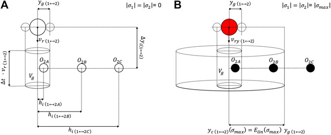
FIGURE 1. Binary collisions between settling objects of different size: (A) neutral objects; (B) objects charged at the ionization limit. In all the Figures, O2A, O2B represent three possible positions of the object O2; yg and yc represent the geometrical and the critical distance respectively; Δyi represents the initial vertical offset between the objects, and hi represents the initial horizontal offset; vr is the relative velocity between the objects which is the settling velocity of O1 in the reference system jointed to O2.
Therefore, the volume swept by an object O1 with respect to O2 can be defined as the volume to which the centre of O2 needs to belong for collision to happen. When the objects O1 and O2 are oppositely charged, they will move toward each other horizontally under the effect of Coulomb attraction. As a result, they can collide with each other even if their horizontal offset is higher than the geometrical distance
In order to quantify the effect of charge on collision efficiency, it is useful to consider the maximum volume
As shown in Figure 1B, both the volumes
This approximation allows us to predict whether two particles will collide or not based on their horizontal offset only.
Objects will eventually collide provided that their horizontal offset is lower than the critical distance
The symbol
While the electrical collision efficiency quantifies the increase in the swept volume for charged objects with respect to neutral ones, its square root, which we can call linear collision efficiency, quantifies the increase in the critical distance:
When the electrical collision efficiency is greater than one, electrical forces have the effect of enhancing object collision; conversely, when the linear electrical collision efficiency is lower than 1, electrical forces decrease collisions. These two possibilities correspond respectively to the case of oppositely charged objects
In this study, we will focus on the case of oppositely charged objects, which constitute the vast majority of the objects that will eventually collide. In fact, as we will show in the results, the electrical collision efficiency is always higher than one for oppositely charged objects, and can reach values between 100 and 1,000 for collisions between objects of a few micrometres (as we will show in the result section). Conversely, collision efficiency is always lower than one for likely-charged objects, as the critical distance is lower than the geometrical distance. Therefore, the vast majority of couples of objects that undergo collisions is represented by oppositely-charged objects. This is especially true for micron-sized objects for which the ratio between the collision efficiency for oppositely charged objects and the collision efficiency for likely charged objects can be higher than 1,000. Since micron-sized objects are the ones that are more likely to stick with each other, in this study we focus on collisions between oppositely charged objects only.
The volumetric flow rate of colliding objects is represented by the following equation for the collision kernel
In general, the vertical component of the relative velocity
If we know the linear collision efficiency for a couple of objects, we can multiply it by the geometrical distance and obtain the critical distance. The linear collision efficiency depends on both the size of the considered objects and their surface charge. If the surface charge is a value between zero and the value at the ionization limit, the collision efficiency will be somewhere between the collision efficiency for neutral objects and the collision efficiency for objects charged at the ionization limit. In this study, the linear collision efficiency will be computed for volcanic objects for different size combinations and surface charges.
Neglecting hydrodynamic interactions between the objects and the lift forces, the objects move under the effect of their weight, their mutual Coulomb attraction
For a given vertical and horizontal offset between two objects, numerical solution of the system of differential equations can provide the relative position through time, and, therefore, allows us to predict whether the two objects will collide. However, the occurrence of collision is dependent on both the initial vertical offset and the initial horizontal offset between the objects. It is worth noticing here that whatever the vertical offset, two objects of different sizes will eventually reach the same altitude. Therefore, the occurrence of collision will mainly depend on their initial horizontal offset.
In fact, assuming no hydrodynamic interactions, it is reasonable to expect that oppositely charged objects characterised by different terminal velocities will eventually collide provided that their horizontal offset is small enough, regardless of their starting altitude. Similarly, given the impossibility of carrying an infinite amount of charge, it is reasonable to assume the probability of collision to be zero if their initial horizontal offset is high enough, regardless of their initial vertical offset.
Moreover, for a given charge and a given initial horizontal offset, the lower the relative velocity between the objects, the higher the probability of collision. In fact, when the objects settle at a similar terminal velocity, Coulomb forces have more time at their disposal to accelerate the objects toward each other. Therefore, we estimate the critical horizontal offset by comparing two timescales: the exposure time
Assuming spherical objects characterised by an evenly distributed surface charge, their net charges are
where
where
and the drag coefficients for spherical objects can be obtained with the formula proposed by Clift and Gauvin (1971):
where the Reynolds number needs to be computed for each object:
Where
where R represents the radius of the sphere and
Therefore, the maximum charge that an object can carry in air is given by:
If we assume that the charge is uniformly distributed on the sphere’s surface, we can compute the maximum surface charge density:
Considering a dielectric strength of 3
For every couple of objects, the critical distance was numerically computed finding the maximum initial horizontal offset between the objects for which the collision time was lower than the exposure time. In order to obtain the critical distance, for each couple of sizes, a starting distance equal to 100 times the sum of object radii was considered, and the collision time was computed and compared to the exposure time. The value of the distance was then updated with an iterative procedure based on the bisection method.
Dividing the value of the critical distance by the sum of the object radii, we obtained the linear collision efficiency for different colliding objects. This allowed us to draw collision maps (see following section). When collision occurs, two outcomes are possible: either the objects stick, or they rebound. Sticking will happen provided that the relative velocity
The sticking velocity for dry objects can be computed with the formula proposed by Thornton and Ning (1998):
Where
Combining Eq. 13 with numerical simulations, Chen et al. (2015) obtained an algorithm to compute the sticking velocity which takes also viscoelastic deformation into account. It is worth noting that the values of the sticking velocity computed for viscoelastic particles are higher respect to the ones given in Eq. 13. In fact, while Eq. 13 takes into account for energy dissipation given by adhesive forces, the algorithm proposed by Chen et al. (2015) takes also into account for energy dissipations associated with viscoelastic behaviour of the objects.
In order to obtain upper estimate of the sticking velocity, in this paper we consider the objects to have a viscoelastic behaviour, and therefore we employ the algorithm of Chen et al. (2015) to estimate the sticking velocity. As input parameters, the algorithm of Chen et al. (2015) requires
It is worth noting that the employed model for computing the sticking velocity is no longer valid if large water layers form around volcanic particles. In fact, if water layers whose thickness is high compared to the surface roughness form around colliding objects, drag forces associated with water layer become the dominant dissipation mechanism. Therefore, the sticking velocity associated with significant water layers is higher than the one considered in this work. Moreover, experimental investigations show that electrification is decreased in wet conditions (Stern et al. (2019)).
If the thickness of the water layer is known, the sticking velocity could be computed with the model proposed by Ennis et al. (1991). However, estimation of water layers go beyond the scope of this work.
Comparing the sticking velocity with the relative velocity, we obtained the sticking maps, which allow us to identify the size combinations that lead to particle sticking.
Results
The relative velocity and the sticking velocity were computed for many combinations of object diameter
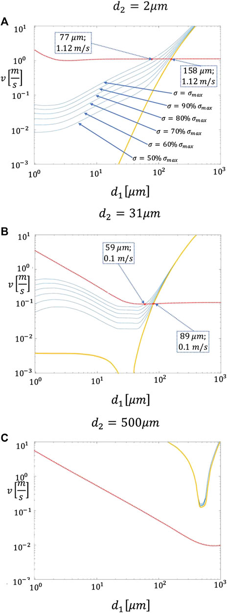
FIGURE 2. Sticking velocity and relative velocity as a function of diameter for couples of objects colliding at 10 km and characterised by a density of 2500
Plots similar to Figure 2 can be compiled for many other size combinations in order to produce a sticking map and verify whether two objects that collide will also stick. However, prior to a sticking map, we need to compile a collision map to verify whether two objects will collide (e.g. Figure 3A). Every point of the plane in Figure 3A corresponds to a couple of interacting objects whose diameters are d1 and d2. Both objects are considered to be oppositely charged at the ionization limit and are characterised by a density of 2500 kg/m3 (so this specific map is mostly suited to describe collision of ash particles more than aggregates). The collision altitude is set to 10 km. For every point of the plane, the linear collision efficiency was calculated dividing the critical distance by the sum of the radii of the colliding objects. The map shows that the linear collision efficiency increases rapidly for smaller objects (red region), it converges to one for larger objects (blue region) and it is symmetrical with respect to the bisector. Moreover, linear collision efficiency is higher toward the bisector, where the colliding objects are characterised by similar sizes, and, thus, similar terminal velocities. Solutions along this line were not computed: as a matter of fact, such collisions are characterised by a collision efficiency which is either zero or infinite, depending on their initial vertical offset. This is due to the fact that objects of the same size settle at the same terminal velocity. Therefore, if they are characterised by the same initial altitude, they theoretically have an infinite amount of time to approach each other under the effect of Coulomb attraction, leading to a collision regardless of the initial horizontal offset. On the other hand, if the objects initial altitude is different, they will never collide.
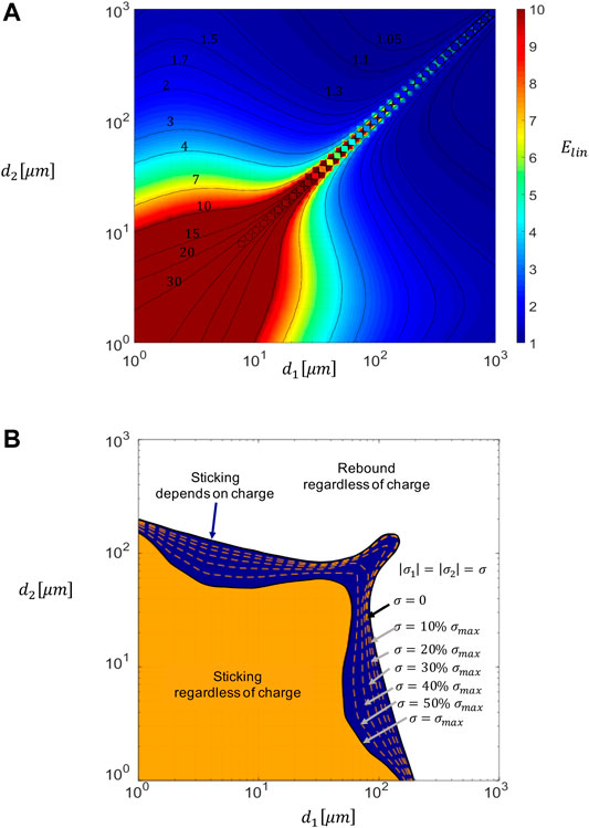
FIGURE 3. (A) Linear collision effciency map and (B) sticking map for objects charged at their ionization limit colliding at 10 km characterized by a density of 2500
In order to compile sticking maps (Figure 3B), plots similar to Figure 2 were compiled for 100 different size combinations. In the Supplementary Material, we also report sticking maps for different values of object densities (ranging between 1,000 kg/m3 and 2500 kg/m3); altitude (ranging between 5 and 15 km); and surface energy (ranging between 15 mJ/m2 and 25 mJ/m2). Figure 3B shows the sticking map for both neutral and charged objects. While Figure 3A describes whether two objects collide or not, Figure 3B predicts if the two objects stick or not. The diameters d1 and d2 of the colliding objects identify a point on the plot of Figure 3B Since the outcome of the collision between two objects of given sizes depends on their charge, several lines are drawn on the plot. Such lines divide the sticking region by the rebound region and are relative to different values of the object charges. If colliding objects are neutral, the external line is to be considered; if objects are oppositely charged at the ionization limit, the internal line is to be considered. If objects surface charge is a percentage of that at the ionization limit, the corresponding dashed line needs to be considered. Once both the points that correspond to the sizes of the colliding objects and the line that corresponds to object charge are identified, the collision outcome can be predicted by their relative position: if the point is in the internal region delimited by the boundary line, colliding objects will stick; if the point is on the external region, colliding objects will rebound. In order to appreciate the effect of charge on collision outcome, it is worth noticing that the boundary lines divide the quadrant in three regions. One in which colliding objects will always rebound regardless their charge (white region); one in which objects will always stick regardless of their charge (orange region), and one in which the collision outcome depends on the charge (blue region).
Since every aggregate is the result of a series of binary collisions between objects that ended up in sticking, its evolution can be described provided that the occurrence and the outcome of every collision can be predicted. A collision map (e.g. Figure 3A) can be compiled based on the density of the colliding objects, the magnitude of their surface charges and the altitude at which collision happens. Nonetheless, in order to compile a sticking map (i.e. Figure 3B), the surface energy of the object also needs to be known. In particular, if both the initial horizontal offset between the objects are known, Figures 3A,B can be used to determine whether the objects will collide, and to predict whether they will stick. While the collisions occurrence can be determined with Figure 3A, the collision outcome (sticking or rebound) can be determined with Figure 3B.
The formation of an aggregate is characterised by a succession of several collisions that end up in sticking. In order to illustrate how collision and sticking maps can be used to describe aggregate evolution in the case of a cored cluster (an aggregate formed by a larger particle in the middle surrounded by a crust of finer particles), we consider the simple case of a core object (i.e. individual particle) falling through a homogeneous cloud of smaller particles characterised by a bimodal grain size distribution (Figure 4). If the real grain size distribution in known, the same reasoning can be repeated for all the possible size combinations. Let the core’s diameter be
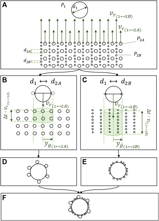
FIGURE 4. Schematic representation of neutral particles forming a cored cluster. (A) core particle falling through a cloud of smaller particles, characterised by a bimodal grainsize distribution. Velocity vectors are shown in the reference system of the larger particle. (B) swept volumes relative to the interactions between P1 and P2A, (C) swept volumes relative to the interactions between P1 and P2B; in both Figures (B),(C), the velocities are drawn with respect to the reference system of P2. Figures (D),(E) show the particles that stick with the core. (F) final cored cluster (i.e. initial core particle surrounded by a variety of particles P2A and P2B).
Let us now consider the same case for charged particles sketched in Figure 5. In this case, a horizontal component of the relative velocity will arise due to electrical attraction, as shown in Figure 5. However, the effect of the horizontal component on the relative velocity, is already taken into account behind the computation of the collision and sticking maps. For this reason in Figures 5B,C we only consider the vertical component of the relative velocity, which is given by the difference between the terminal velocities.
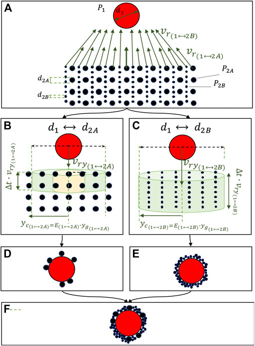
FIGURE 5. Schematic representation of oppositely charged particles forming a cored cluster. The red particle is positively charged at the ionization limit, the black particles are negatively charged at the ionization limit. (A) core particle falling through a cloud of smaller particles, characterised by a bimodal grainsize distribution. Velocity vectors are shown in the reference system of the larger particle. (B) swept volume (in green) relative to the interactions between P1 and P2A (sticking volume is represented in orange), (C) swept volume (in green) relative to the interactions between P1 and P2B. In both Figures (B) and (C), the velocities are drawn with respect to the reference system of P2. (D) and (E) show the particles that stick with the core. (F) final cored cluster (i.e. initial core particle surrounded by a variety of particles P2A and P2B).
In Figure 5B two volumes are identified. The green one represents the collision volume inside which particles will collide. Comparing Figure 5B with Figure 4B one can appreciate the increase in the collision volume for charged particles with respect to neutral particles. However, out of all the particles that will eventually collide only the ones inside the yellow volume will end up in sticking. In fact, particles that are inside the green volume and outside the yellow volume have more room to accelerate under the effect of Coulomb interaction. For this reason, they collide at a velocity that is too high for sticking to happen. The radius of the green volume corresponds to the critical distance, which can be calculated from the linear collision efficiency given by Figure 3A. The radius of the yellow volume is the sticking distance, which we define has the horizontal offset below which particles will eventually collide and stick.
Linear collision efficiency for the interaction between the core and 15 µm particles is E(1–2A) = 2.5. For the interaction between the core and the 1 µm particles, it is E(1–2B) = 3.4. The increase in the swept volume for the particles charged at the ionization limit with respect to the neutral case is given by Eq. 2. Substituting the numbers, we obtain that the volume increases 6.25 times for the interaction between the core and 15 µm particles, and it increases 11.56 times for the interaction between the core and 3 µm particles. Finding the points that correspond to particle diameters on Figure 3B, we see that the core will always stick with 1 µm particles.
Discussion
Our analysis shows that both the collision efficiency and the sticking efficiency of settling objects can be predicted computing collision maps and sticking maps (e.g. Figures 3A,B). Although both maps are computed for a given collision altitude (10 km), a given object density (2500 kg/m3), and the sticking map is drawn for given surface tension (20 mJ/m2), their shape allow to draw some general qualitative conclusions about aggregation of settling volcanic particles and aggregates.
Numerical Simulations vs Analytical Solutions
Although charge dependent approximated formulas could be theoretically derived for both collision efficiency and sticking efficiency, the presence of velocity dependent drag forces (Eq. 6) for a wide range of Reynolds numbers (Eq. 9) makes it impossible to find an analytical closed form solutions. For this reason, we opted for numerical simulations. Even in the case in which drag forces can be considered negligible with respect to electrical forces, analytical solutions for the collision efficiency are rather challenging, but not impossible. In fact, the motion of two objects in an inverse-square field is known in classical mechanics as the two-body problem, which has analytical solutions. Although a complete theoretical solution is beyond the scope of this paper, in Appendix A, B we lay out the foundation for such a derivation. Moreover, in the Supplementary Material we employ an analytical expression for the collision velocity to derive equations to apply the sticking maps to objects released at an arbitrary initial offset.
Increase in Collision Frequency: Impact of Object Charge and Size
The collision map (Figure 3A) shows that the collision efficiency is dramatically enhanced for small objects (<10 μm) charged at the ionization limit. This is mainly due to their low inertia, which allows Coulomb forces to effectively accelerate the objects toward each other. Moreover, the enhancement effect of Coulomb forces is more important when the oppositely charged objects have similar sizes. This is due to the fact that objects characterised by similar sizes also have similar terminal velocities, and, therefore, a lower relative velocity. As a result, they stay close to each other for long enough for the electrical forces to act. However, it is worth noting that objects of similar size that have undergone triboelectric charging are likely to carry charges of the same polarity (Lacks and Levandovsky (2007)). Therefore, despite the fact that the highest enhancement of collision efficiency is theoretically obtained for two small (<10 μm) oppositely charged objects of similar size, in reality the highest enhancement may be reached when just one of the colliding objects is small (<10 μm).
In fact, numerous experimental studies have indicated that contact electrification/triboelectrification preferentially charges small objects negatively and large objects positively as a consequence of collision (e.g. Lacks and Levandovsky, 2007; Alois et al., 2017). Such a size dependence in polarity would enhance the creation of aggregates due to attraction of small (negative) objects to large (positive) objects compared to the case where there is no size dependence.
The effect of object size on collision can be seen comparing Figures 4B,C. When the collected object is small (Figure 4C), the volume swept per unit time stretches vertically due to the higher relative velocity and shrinks laterally due to the smaller geometrical distance. The second effect is dominant with respect to the first one. Opposite charge has the effect of dramatically increasing the swept volume. As can be seen comparing Figure 5B with Figure 4B, and Figure 5C with Figure 4C, the volume increase is more important when the collected object is small. The result is that small objects will collide more than large objects, despite the lower geometrical distance.
Reduction of Sticking Efficiency: Impact of Object Charge, Size, Density, Surface Energy and Collision Altitude
Figure 3B shows that collision between small objects (i.e. all the size combinations relative to the golden area of Figure 3B) end up in sticking regardless of their charge. This happens because their mass is low enough for the collision kinetic energy to be dissipated. On the other hand, collisions between the objects characterised by the size combinations in the blue area of Figure 3B stick to each other only if the colliding objects are neutral. This happens due to their low collision velocity, which keeps the collision kinetic energy lower than the threshold value for sticking. This study shows that on one hand the presence of an opposite charge on objects always determines more collisions compared to neutral objects (see Figure 3A, where the linear collision efficiency is always greater than 1), and on the other hand it decreases the sticking efficiency for big objects. Moreover, depending on object size, charged objects might not stick with each other even when their neutral counterparts would stick (Figure 5B). This is caused by the increase in relative velocity that occurs just before collision due to Coulomb interactions. However, this result is based on the assumption that electrical forces do not affect the sticking velocity between objects. The lower sticking region of charged objects can be quantitatively described by the ’sticking volume’ shown in Figure 5B, which is smaller than the swept volume. The combination of the effects of charge on sticking and collision ultimately lead to a finer grain-size distribution for charged aggregates (Figures 4F, 5F). This occurs not only due to the significant increase in the collected smaller particles, but also as a result of a higher number of larger particles that collide and rebound.
Since the sticking behaviour of objects is strongly dependent on their density, in Appendix C we show how these parameters affect the sticking maps. Results allow to quantitatively explain some known facts about volcanic particle aggregation. Firstly, the higher the surface energies, the bigger the size of the objects that can stick (Figure 3C; Appendix C). This explains why wet aggregates, which are characterised by high surface energies, contain large particles (i.e. coarse ash). Secondly when collisions happen at lower altitudes, larger particles can stick (Figure 2C; Appendix C). This happens because if objects collide at low altitudes, their relative velocity is lower due to the higher density of the surrounding fluid. The implication of this is that the altitude at which aggregates form has an effect on the internal grain-size distribution. Finally, when the colliding objects have lower densities, larger particles can stick (Figure 1C; Appendix C). This is one of the reasons why for the same given size two aggregates are more likely to stick than two particles.
In conclusion, besides providing a quantification of the effect of charge, the obtained collision and sticking maps represent a powerful tool to quantitatively describe the effect that all the possible parameters can have on aggregation of volcanic particles and aggregates.
Collision and Sticking Maps: Limits of Applicability
The model proposed in this paper describes collisions between dry objects, which take place during particle sedimentation in still air. However, the maps (Figures 3A,B) provide meaningful constrains also when the conditions mentioned above are not fully satisfied. In order to clarify these constrains, we review and discuss each assumption behind the model.
The “still air” assumption (i.e. no wind and no turbulence) allowed us to compute the relative velocities between the objects considering only the combined effect of differential settling, Coulomb forces and drag forces. When the effect of wind and turbulence are not negligible, the relative velocities between the colliding objects may be higher with respect to the ones predicted in our model. As a result, wind and turbulence may increase the collision efficiency and decrease the sticking efficiency. Therefore, when the “still air” assumption is not verified the collision map (Figure 3A) may provide a lower bound to the collision efficiency, and the sticking map (Figure 3B) may provide an upper bound to the sticking efficiency.
Since Brownian motion and fluid shear were not considered in the model, the maps are applicable to size combinations for which differential settling is the dominant collision mechanisms. This is true provided that the smallest object is larger than 1
Since our model focuses on dry aggregation, it can be directly applied provided that the relative humidity of the surrounding environment is lower than 71%. In fact, according to Telling et al. (2013) this is the threshold value beyond which water films start to form on the objects. If the mass of the water layers is negligible with respect to the mass of the particles, the collision map is still applicable. Regarding the sticking map (Figure 3B), it can still be applied to obtain a conservative estimation of the sticking efficiency as wet objects stick more easily than dry objects.
Since spherical objects of the same density are characterised by the same settling velocity, our model is not applicable to collisions between objects of similar size. In fact, the maps (Figures 3A,B) were obtained considering only couples of objects such that the largest one is at least 10% larger than the smallest one. Therefore, the points around the bisector should not be considered when applying either map (Figures 3A,B).
It is worth reminding here that the collision map (Figure 3A) and the sticking map (Figure 3B) were obtained considering that both the objects are colliding at an altitude of 10 km above sea level, they are characterised by a density of
Furthermore, when applying our model to real particles, we need to take into consideration the fact that their charge might exceed the maximum surface charge, and we need to be aware of the implications of an irregular shape. These effects are discussed below for both the collision and the sticking maps. Regarding the collision map (Figure 3A), it is directly applicable when the colliding objects are oppositely charged with surface charges of
Moreover, since irregular objects will have in general higher drag forces than spherical ones (Bagheri and Bonadonna, 2016), the values given in Figure 3A constitute an upper limit for the linear collision efficiency of real objects. Regarding the sticking map, the fact that fine particles can carry surface charges that are higher than 27
Since our model considers differential settling to be the dominant collision mechanism, the provided maps cannot be directly applied inside the volcanic plume, where turbulence plays an important role. Computation of collision and sticking maps inside the plume requires the knowledge of relative velocity for all the size combinations. Since these velocities strongly depend on the eruption parameters, it is not possible to obtain maps of general validity.
However, the qualitative results regarding the effect of oppositely charged objects with respect to neutral ones might still hold within the volcanic plumes and clouds. In fact, all the other parameters being equal, oppositely charged objects will always lead to an increase in the swept volume, and an increase in the relative velocity with respect to neutral objects and similarly charged objects. Therefore, we expect that charged objects lead to the formation of aggregates which are richer in fine ash regardless of the environment where they form (plume, cloud, or atmosphere).
Field Observations of Oppositely Charged Objects and Aggregate Grain Size that Support the Proposed Model
The conclusion that charged objects form aggregates which are richer in fine ash has general validity provided that oppositely charged objects are present in the volcanic plume and cloud, and that most collisions occur between oppositely charged objects. The presence of oppositely charged particles is confirmed by the field observations performed by Miura et al. (2002), which show that the charging mechanism seems to be size dependent, leading to scenarios such as the one sketched in Figure 1B. The fact that most collisions occur between oppositely charged particles is a consequence of the fact that couples of particles carrying the same charge sweep a smaller volume than both neutral and oppositely charged particles.
In order to show how our model can be applied to a volcanic context, we reviewed several grain-size distributions available in literature. To date, grain-size distributions have been determined for all aggregate types (e.g. Bagheri et al. (2016); Bonadonna et al. (2002); Bonadonna et al. (2011); Brazier et al. (1982); Burns et al. (2017); van Eaton and Wilson (2013)). In particular, Bagheri et al. (2016) presented the grain-size distribution of cored clusters formed at Sakurajima volcano. As an example, we consider one of the aggregates they identified which was composed of a 250 µm core, and a shell which included particles between 8 and 44 µm. If both the particle surface energy and the colliding altitude were known, a sticking map could be compiled in order to see whether the grain-size distribution is compatible with the scenario of an aggregate formed during settling. Assuming the conditions of Figure 3B (i.e. a surface energy for dry particles of 20 mJ/m2, which is the value for silica, and a particle density of 2500 kg/m3, which is the mean particle density measured by Bagheri et al. (2016)) a 250 µm particle would not be able to stick with any other particle. Therefore, aggregate formation must have started in an environment where particles had either a higher surface energy, maybe due to high humidity, or lower relative velocity. It is likely that the 250 µm particle has found such conditions in the higher portion of the plume, where the plume mixture might have reached the saturation point, and water layers might have formed around the particles, determining a high surface energy. Indeed, by measuring the settling time of aggregates, Bagheri et al. (2016) also estimated that aggregates were likely to be formed in the higher part of the plume.
Collision Frequency: The Impact of Particle Concentration
The map in Figure 3A provides the normalised critical distance, which is the ratio between the critical distance and the sum of the radii of colliding particles. The electrical collision efficiency, which quantifies the enhancement of the swept volume due to Coulomb interactions, can be obtained by computing the square of the normalised critical distance. For example, a normalised critical distance of 30 implies that charged objects sweep an effective volume that is 900 times larger than the volume swept by neutral particles. In addition, the collision kernel can be computed by multiplying the collision efficiency by the geometrically swept area and the relative velocity in order to constrain the volumetric flow rate of colliding particles (Eq. 3). As discussed in previous sections, aggregation of volcanic particles strongly depends on both collision efficiency and sticking efficiency. In particular, collision rate with respect to any particular object (i.e. amount of collisions per unit time) depends on particle number concentration n (i.e. number of particles per unit volume):
If both the mass concentration and the mass fractions are known, the particle number concentrations can be computed for every size combination. The concentration of particles associated with volcanic eruptions depends on several factors such as the eruption physical parameters, the meteorological conditions, the altitude of the plume/cloud and the distance from the vent. An example of how particle concentration charges with altitude is provided by Moxnes et al. (2014), who report measurements of ash concentration over Stockholm after the 2011 Grimsvötn eruption (Iceland). Their profiles show that mass concentration varies between 0 and 300
In-situ investigations carried out between 9 and 11 May 2010 during the eruption of Eyjafjallajökull (Iceland) showed that ash concentration at 45–60 km from the vent was below 53 μg/m3 outside the plume and could reach 2000 μg/m3 at the outskirt of the volcanic cloud (Weber et al. (2012)).
In order to show the effect of electrical forces on collision rate, we calculated the particle number concentration associated with different particle size employing the grain-size distribution derived from both field and remote-sensing information (Table 1), and assuming spherical particles with a density of 2500 kg/m3. We computed the number of collisions per day for a 10 μm particle interacting with other particles between 1 and 100 μm (Figures 6A,B). Computations were done for three order of magnitudes of concentrations (10 μg/m3, 100 μg/m3, 1,000 μg/m3), and for the concentrations measured by Weber et al. (2012) at Eyjafjallajökull (53 μg/m3, 2000 μg/m3). The enhancement in the collision rate due to electrical forces is clearly more important for fine particles (Figure 6).
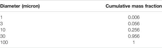
TABLE 1. total grain size distribution associated with the eruption of Eyjafjallajökull (2010) between 5–8 May 2010, (Bonadonna et al. (2011))
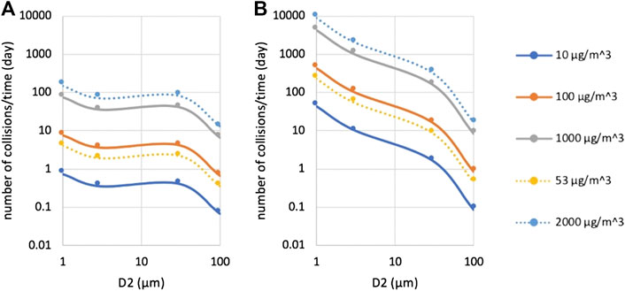
FIGURE 6. Collision rate with respect to one specific particle whose diameter is D1 = 10 mm, interacting with another particle whose diameter is represented by D2. Different lines correspond to different concentration values. While solid lines show three different orders of magnitudes (10 μg/m3, 100 μg/m3, 1,000 μg/m3); dashed lines are relative to the values measured by Weber et al. (2012) in May 2010 at Eyjafjallajökull (Iceland) (see text for details). (A) is relative to neutral particles; (B) is relative to oppositely charged particles at the ionization limit.
Conclusions
Numerical simulations have been performed to study the effect of charge on aggregation of settling ash in still air. Since an aggregate is formed as a result of a series of binary collisions, we considered the interactions between couples of objects (i.e. either particles or aggregates). For a given altitude, object density and surface energy, a collision map (Figure 3A) and a sticking map (Figure 3B) were obtained to predict whether a couple of objects will collide and stick with each other.
The collision map (e.g. Figure 3A) shows that oppositely charged objects are more likely to collide than neutral ones as they sweep a larger volume. In particular, the increase in swept volume is progressively more important for smaller objects of similar sizes. However, since objects of similar size are likely to carry charges of the same polarity due to the nature of triboelectric charging, the couples of objects that benefit the most from an electrically driven enhancement in collision efficiency are the ones that involve one small object (<10
Moreover, the sticking map (e.g. Figure 3B) allows to determine the collision outcome for both neutral and oppositely charged colliding objects. In particular, it shows that if colliding objects are small enough (<20
Given that aggregates form as a result of a series of binary collisions that end up in sticking, the combined use of collision and sticking maps allows to quantify the effect of charge on grain size distribution. Since the enhancement in collision efficiency is more important when one of the colliding object is small
If both particle concentration and grain-size distribution in the atmosphere are known, the collision map can be used to estimate the number of collisions per unit time that a particular object experiences. Such a number was computed for the 2010 eruption of Eyjafjallajökull under the assumption of constant ash concentration in the atmosphere (See Figures 6A,B). Considering the interaction between a 1 μm and a 10 μm object as an example, we showed that neglecting the effect of charge leads to underestimating by almost three orders of magnitude the number of collisions.
Even though our analysis focuses on aggregation of objects settling in still air, the same framework can be extended in future studies to study aggregation in the volcanic plume and cloud, where the combined effect of Coulomb forces and turbulent forces needs to be considered. Although more experimental investigations are needed to establish the exact values of both the collision efficiency and the threshold sizes for sticking of volcanic objects, our study provides a way to quantify the magnitude of the effects of charge on aggregation processes, which should be taken into account in future aggregation models.
Although electric charge affects both collision and sticking efficiency (as shown in Figures 3A,B), considering even only the effect of charge on collision efficiency would be enough to considerably improve the estimates of fine ash concentration in the atmosphere. In fact, neglecting object charge leads to a significant overestimation of the amount of fine ash that remains airborne. Since accurate estimations of fine ash concentration in the atmosphere are necessary to mitigate volcanic risk, it is of primary importance that aggregation models take at least the effects of electrification on collision efficiency into account.
Data Availability Statement
The original contributions presented in the study are included in the article/Supplementary Material, further inquiries can be directed to the corresponding author.
Author Contributions
SP conducted this work as part of his Ph.D. He developed the theoretical framework and performed the numerical simulations under the supervision of CB and ER. JM largely contributed to the interpretation of the results. All authors were involved in the finalization of the manuscript.
Funding
This work was supported by the Swiss National Science Foundation (grant number 200021_156255).
Conflict of Interest
The authors declare that the research was conducted in the absence of any commercial or financial relationships that could be construed as a potential conflict of interest.
Acknowledgments
We would like to thank Giovanni Macedonio and Corrado Cimarelli reviewers for insightful comments and suggestions.
Supplementary Material
The Supplementary Material for this article can be found online at: https://www.frontiersin.org/articles/10.3389/feart.2020.574106/full#supplementary-material.
References
Aizawa, K., Cimarelli, C., Alatorre-Ibargüengoitia, M. A., Yokoo, A., Dingwell, D. B., and Iguchi, M. (2016). Physical properties of volcanic lightning: constraints from magnetotelluric and video observations at Sakurajima volcano, Japan. Earth Planet Sci. Lett. 444, 45–55. doi:10.1016/j.epsl.2016.03.024
Alois, S., Merrison, J., Iversen, J. J., and Sesterhenn, J. (2017). Contact electrification in aerosolized monodispersed silica microspheres quantified using laser based velocimetry. J. Aerosol Sci. 106, 1–10. doi:10.1016/j.jaerosci.2016.12.003
Bagheri, G., and Bonadonna, C. (2016). On the drag of freely falling non-spherical particles. J. Powder Technology 301, 526–544. doi:10.1016/j.powtec.2016.06.015
Bagheri, G., Rossi, E., Biass, S., and Bonadonna, C. (2016). Timing and nature of volcanic particle clusters based on field and numerical investigations. J. Volcanol. Geoth. Res. 327, 520–530. doi:10.1016/j.jvolgeores.2016.09.009
Behnke, S. A., Edens, H. E., Thomas, R. J., Smith, C. M., McNutt, S. R., Eaton, V., et al. (2018). Investigating the origin of continual radio frequency impulses during explosive volcanic eruptions. J. Geophys. Res. Atmosphere 123 (8), 4157–4174. doi:10.1002/2017JD027990
Bonadonna, C., Mayberry, G. C., Calder, E. S., Sparks, R. S. J., Choux, C., Jackson, P., et al. (2002). “Tephra fallout in the eruption of soufrière hills volcano, Montserrat,” in The eruption of soufrière hills volcano, Montserrat, from 1995 to 1999. Editor B. P. Druitt TH Kokelaar (London, Memoir: Geological Society), 21, 483–516
Bonadonna, C., Genco, R., Gouhier, M., Pistolesi, M., Cioni, R., Alfano, F., et al. (2011). Tephra sedimentation during the 2010 Eyjafjallajökul eruption (Iceland) from deposit, radar, and satellite observations. J. Geophys. Res. Solid Earth 116: B12202. doi:10.1029/2011JB008462
Brazier, S., Davis, A. N., Sigurdsson, H., and Sparks, R. S. J. (1982). Fallout and deposition of volcanic ash during the 1979 explosive eruption of the Soufrière of St-Vincent. J. Volcanol. Geoth. Res. 14, 335–359. doi:10.1016/0377-0273(82)90069-5
Brown, R. J., Bonadonna, C., and Durant, A. J. (2012). A review of volcanic ash aggregation. Phys. Chem. Earth 45–46, 65–78. doi:10.1016/j.pce.2011.11.001
Burns, F. A., Bonadonna, C., Pioli, L., Cole, P. D., and Stinton, A. (2017). Ash aggregation during the 11 february 2010 partial dome collapse of the soufrière hills volcano, Montserrat. J. Volcanol. Geoth. Res. 335, 92–112. doi:10.1016/j.jvolgeores.2017.01.024
Chen, S., Li, S., and Yang, M. (2015). Sticking/rebound criterion for collisions of small adhesive particles : effects of impact parameter and particle size. Powder Technol. 274, 431–440. doi:10.1016/j.powtec.2015.01.051
Cimarelli, C., Alatorre-Ibargüengoitia, M. A., Aizawa, K., Yokoo, A., Díaz-Marina, A., Iguchi, M., et al. (2016). Multiparametric observation of volcanic lightning: Sakurajima Volcano, Japan. Geophys. Res. Lett. 43 (9), 4221–4228. doi:10.1002/2015GL067445
Cimarelli, C., Alatorre-ibargüengoitia, M., Aizawa, K., Scheu, B., and Yokoo, A. (2014). Multi-parametric observation of volcanic lightning produced by ash-rich plumes at Sakurajima volcano. Jpn. Times 16, 34802. doi:10.1130/G34802.1
Clift, W., and Gauvin, R. (1971). Motion of entrained particles in gas streams. Can. J. Chem. Eng. 49 (107), 439–448, doi:10.1002/cjce.5450490403
Costa, A., Folch, A., and Macedonio, G. (2010). A model for wet aggregation of ash particles in volcanic plumes and clouds: 1. Theoretical formulation. J. Geophys. Res. Solid Earth 115, 1–14. doi:10.1029/2009JB007175
Dhanorkar, S., and Kamra, A. K. (1997). Calculation of electrical conductivity from ion-aerosol balance equations. J. Geophys. Res. Atmos. 102, 30147–30159. doi:10.1029/97JD02677
Durant, A. J. (2015). Toward a realistic formulation of fine-ash lifetime in volcanic clouds. Geology 43, 271–272. doi:10.1130/focus032015.1
Elissondo, M., Baumann, V., Bonadonna, C., Pistolesi, M., Cioni, R., Bertagnini, A., et al. (2016). Chronology and impact of the 2011 cordón Caulle eruption, Chile. Nat. Hazards Earth Syst. Sci. 16, 675–704. doi:10.5194/nhess-16-675-2016
Ennis, B. J., Tardo, G, and Pfeffer, R. (1991). A microlevel-based characterization of granulation phenomena. Powder Technol. 65, 257–272. doi:10.1016/0032-5910(91)80189-P
Ferrari, A., Eichenberger, J., and Laloui, L. (2013). Hydromechanical behaviour of a volcanic ash. Geotechnique 63 (16), 1433–1446. doi:10.1680/geot.13.P.041
Gilbert, J. S., Lane, S. J., Sparks, R. S. J., and Koyaguchi, T. (1991). Charge measurements on particle fallout from a volcanic plume. Nature 349, 598–600. doi:10.1038/349598a0
Gilbert, J. S., and Lane, S. J. (1994). The origin of accretionary lapilli. Bull. Volcanol. 56, 398–411. doi:10.1007/BF00326465
Hamamoto, N., and Nakajima, Y. (1992). Experimental discussion on maximum surface charge density of fine particles sustainable in atmosphere. J. Electrost. 28 (2), 161–173. doi:10.1016/0304-3886(92)90068-5
Hatakeyama, H. (1958). On the disturbance of the atmospheric electric field caused by the smoke-cloud of the volcano asama-yama. Pap. Meteorol. Geophys. 8 (4), 302–316. doi:10.2467/mripapers1950.8.4_302
Hatakeyama, H. (1949). On the disturbance of the atmospheric potential gradient caused by the smoke-cloud of the Volcano Yake-yama. J. Meteorol. Soc. Jpn. 27, 372–376. doi:10.5636/jgg.1.48
Hatakeyama, H. (1943). On the variation of the atmospheric potential gradient caused by the cloud of smoke of the volcano asama. Journ. Met.Soc. Japan, Ser. II 21, 420–426. doi:10.2151/jmsj1923.21.2_49
Hatakeyama, H. (1947). On the variation of the atmospheric potential gradient caused by the cloud of smoke of the volcano asama. Journal of the Meteorological Society of Japan. Ser. II 25 (1–3), 3939. doi:10.2151/jmsj1923.21.2_49
Hatakeyama, H., and Uchikawa, K. (1951). On the disturbance of the atmospheric potential gradient caused by the eruption-smoke of the volcano aso. Pap. Meteorol. Geophys. 2 (1), 85–89. doi:10.2467/mripapers1950.2.1_85
James, M. R., Lane, S. J., and Gilbert, J. (1989). The density, construction and drag coefficient of electrostatic volcanic ash aggregates. J. Chem. Inf. Model 53, 160. doi:10.1029/2002JB002011
James, M. R., Lane, S. J., and Gilbert, J. S. (2000). Volcanic plume electrification: experimental investigation of a fracture-charging mechanism. J. Geophys. Res. Solid Earth 105, 16641–16649. doi:10.1029/2000JB900068
James, M. R., Wilson, L., Lane, S. J., Gilbert, J. S., Mather, T. A., Harrison, R. G., et al. (2008). Electrical charging of volcanic plumes. Space Sci. Rev. 137, 399–418. doi:10.1007/s11214-008-9362-z
Lacks, J., and Levandovsky, A. (2007). Effect of particle size distribution on the polarity of triboelectric charging in granular insulator systems. J. Electrost. 65 (2), 107–112. doi:10.1016/j.elstat.2006.07.010
Lund, K. A., and Benediktsson, K. (2011). Inhabiting a risky Earth. Anthropol. Today Off. 27, 6–9. doi:10.1111/j.1467-8322.2011.00781.x
Martin, S. J., Wang, P. K., and Pruppacher, H. R. (1979). A theoretical determination of the efficien cy with which aerosol particles are collected by simple ice crystal plates. J. Atmospheric Sci. 37, 1628–1638. doi:10.1175/1520-0469(1980)037<1628:ATDOTE>2.0.CO;2
Mason, J. (2019). The generation of electric charges and fields in thunderstorms. P. Royal Society of London. Series A, Mathematical and Physical Sciences 415, 303–315. doi:10.1098/rspa.1988.0015
Mather, T. A., and Harrison, R. G. (2006). Electrification of volcanic plumes. Surveys in Geophysics 27, 387–432. doi:10.1007/s10712-006-9007-2
Méndez, J. H., and Dufek, J. (2016). The effects of dynamics on the triboelectrification of volcanic ash. J. Geophys. Res. 121 (14), 8209–8228. doi:10.1002/2015JD024275
Miura, T., Koyaguchi, T., and Tanaka, Y. (2002). Measurements of electric charge distribution in volcanic plumes at Sakurajima volcano. Japan. Bull. Volcanol. 64, 75–93. doi:10.1007/s00445-001-0182-1
Moxnes, E. D., Kristiansen, N. I., Stohl, A., Clarisse, L., Durant, A., Weber, K., et al. (2014). Separation of ash and sulfur dioxide during the 2011 Grímsvötn eruption. J. Geophys. Res. Atmos. 119, 7477–7501. doi:10.1002/2013JD021129
Mueller, S. B., Kueppers, U., Ametsbichler, J., Cimarelli, C., Merrison, J. P., Poret, M., et al. (2017). Stability of volcanic ash aggregates and break-up processes. Sci. Rep. 7, 7440–7511. doi:10.1038/s41598-017-07927-w
Nicoll, K., Airey, M., Cimarelli, C., Bennett, A., Harrison, G., Gaudin, D., et al. (2019). First in situ observations of gaseous volcanic plume electrification geophysical research letters. Geophys. Res. Lett. 46, 3532–3539. doi:10.1029/2019GL082211
Pruppacher, H. R., and Klett, J. (2010). Microphysics of Clouds and Precipitation. Berlin, Germany: Springer, 6826.
Rose, W., and Durant, A. (2009). Fine ash content of explosive eruptions. J. Volcanol. Geoth. Res. 186, 32–39. doi:10.1016/j.jvolgeores.2009.01.010
Schumacher, R. (1994). A reappraisal of Mount St. Helens’ ash clusters - de-positional model from experimental observation. J. Volcanol. Geotherm. Rec. 59, 253–260. doi:10.1016/j.jvolgeores.2009.01.010
Smoluchowski, M. (1917). A mathematical theory of coagulation kinetics of colloidal solutions. Z. Phys. Chem. 92, 129–168
Stern, S., Cimarelli, C., Gaudin, D., Scheu, B., and Dingwell, D. B. (2019). Electrification of experimental volcanic jets with varying water content and temperature. Geophysical Research Letters 46, 11136–11145. doi:10.1029/2019GL084678
Taddeucci, J., Scarlato, P., Montanaro, C., Cimarelli, C., Del Bello, E., Freda, C., et al. (2011). Aggregation-dominated ash settling from the Eyjafjallajökull volcanic cloud illuminated by field and laboratory high-speed imaging. Geology(2011) 29 (9), 891–894. doi:10.1130/G32016.1
Telling, J., and Dufek, J. (2012). An experimental evaluation of ash aggregation in explosive volcanic eruptions. J. Volcanol. Geoth. Res. 209, 1–8. doi:10.1016/j.jvolgeores.2011.09.008
Telling, J., Dufek, J., and Shaikh, A. (2013). Ash aggregation in explosive volcanic eruptions. Geophys. Res. Lett. 40, 2355–2360. doi:10.1002/grl.50376
Thornton, C., and Ning, Z. (1998). A theoretical model for the stick/bounce behaviour of adhesive, elastic-plastic spheres. Powder Technol. 99, 154–162
Van Eaton, A. R., and Wilson, C. J. N. (2013). Nature, origins and distribution of ash aggregation processes in a large-scale wet eruption. J. Volcanol. Geoth. Res. 250, 129–154. doi:10.1016/j.jvolgeores.2012.10.016
Veitch, G., and Woods, A. W. (2001). Particle aggregation in volcanic eruption columns. J. Geophys. Res. Solid Earth 106, 26425–26441. doi:10.1029/2000JB900343
Weber, E., Vogel, F., Pohl, G., van Haren, M., Meier, B., and Grobéty, D. (2012). Airborne in-situ investigations of the Eyjafjallajökull volcanic ash plume on Iceland and over north-western Germany with light aircrafts and optical particle counters. Atmos. Environ. 48, 9–21. doi:10.1016/j.atmosenv.2011.10.030
Keywords: volcanic particle aggregation, electrification, collision efficiency, sticking efficiency, collision map
Citation: Pollastri S, Rossi E, Bonadonna C and Merrison JP (2021) Modelling the Effect of Electrification on Volcanic Ash Aggregation. Front. Earth Sci. 8:574106. doi: 10.3389/feart.2020.574106
Received: 18 June 2020; Accepted: 07 December 2020;
Published: 12 February 2021.
Edited by:
Antonio Costa, National Institute of Geophysics and Volcanology (Bologna), ItalyReviewed by:
Giovanni Macedonio, Istituto Nazionale di Geofisica e Vulcanologia (INGV), ItalyCorrado Cimarelli, Ludwig Maximilian University of Munich, Germany
Copyright © 2021 Pollastri, Rossi, Bonadonna and Merrison. This is an open-access article distributed under the terms of the Creative Commons Attribution License (CC BY). The use, distribution or reproduction in other forums is permitted, provided the original author(s) and the copyright owner(s) are credited and that the original publication in this journal is cited, in accordance with accepted academic practice. No use, distribution or reproduction is permitted which does not comply with these terms.
*Correspondence: Stefano Pollastri, U3RlZmFuby5Qb2xsYXN0cmlAdW5pZ2UuY2g=