 William S. D. Wilcock1*
 Dana A. Manalang2
 Erik K. Fredrickson1
 Michael J. Harrington2
 Geoff Cram2
 James Tilley2
 Justin Burnett2
 Derek Martin2
 Taro Kobayashi3
 Jerome M. Paros3
- 1School of Oceanography, University of Washington, Seattle, WA, United States
- 2Applied Physis Laboratory, University of Washington, Seattle, WA, United States
- 3Paroscientific, Inc., Redmond, WA, United States
Geodetic observations in the oceans are important for understanding plate tectonics, earthquake cycles and volcanic processes. One approach to seafloor geodesy is the use of seafloor pressure gauges to sense vertical changes in the elevation of the seafloor after correcting for variations in the weight of the overlying oceans and atmosphere. A challenge of using pressure gauges is the tendency for the sensors to drift. The A-0-A method is a new approach for correcting drift. A valve is used to periodically switch, for a short time, the measured pressure from the external ocean to the inside of the instrument housing at atmospheric pressure. The internal pressure reading is compared to an accurate barometer to measure the drift which is assumed to be the same at low and high pressures. We describe a 30-months test of the A-0-A method at 900 m depth on the MARS cabled observatory in Monterey Bay using an instrument that includes two A-0-A calibrated pressure gauges and a three-component accelerometer. Prior to the calibrations, the two pressure sensors drift by 6 and 2 hPa, respectively. After the calibrations, the offsets of the corrected pressure sensors are consistent with each other to within 0.2 hPa. The drift corrected detided external pressure measurements show a 0.5 hPa/yr trend of increasing pressures during the experiment. The measurements are corrected for instrument subsidence based on the changes in tilt measured by the accelerometer, but the trend may include a component of subsidence that did not affect tilt. However, the observed trend of increasing pressure, closely matches that calculated from satellite altimetry and repeat conductivity, temperature and depth casts at a nearby location, and increasing pressures are consistent with the trend expected for the El Niño Southern Oscillation. We infer that the A-0-A drift corrections are accurate to better than one part in 105 per year. Additional long-term tests and comparisons with oceanographic observations and other methods for drift correction will be required to understand if the accuracy the A-0-A drift corrections matches the observed one part in 106 per year consistency between the two pressure sensors.
Introduction
On land, dense geodetic observations from global navigation satellite systems and interferometric synthetic aperture radar have transformed our understanding of plate tectonics, earthquake cycles and volcanic processes (Bürgmann and Thatcher, 2013; Doglioni and Riguzzi, 2018). On the seafloor, geodetic observations are more challenging because seawater does not propagate electromagnetic waves, but they are nevertheless important (Bürgmann and Chadwell, 2014; Fujimoto, 2014). Most of the Earth’s volcanism occurs underwater and most plate boundaries lie within the oceans or near coastlines, including subduction zones that host the largest and many of the most destructive earthquakes. To characterize and mitigate seismic and tsunami risk, seafloor geodesy is needed in subduction zones to determine where the faults are locked and where they are partially or completely slipping by steady creep or episodic slow slip (e.g., Wang and Tréhu, 2016). Seafloor geodesy is also necessary for improving our understanding of the dynamic processes at ocean spreading centers, transform faults and hotspot volcanoes (e.g., Chadwell et al., 1999; Chadwick et al., 2006; McGuire and Collins, 2013). Furthermore, along some coastlines, geodetic observations are of potential importance for monitoring the stability of submarine slopes (Blum et al., 2010).
There are several established methods for seafloor geodesy (Bürgmann and Chadwell, 2014; Fujimoto, 2014) and extensive research efforts are underway to develop new techniques (e.g., Zumberge et al., 2018; DeSanto and Sandwell, 2019). One longstanding approach is the use of seafloor pressure gauges to sense vertical changes in the elevation of the seafloor after correction for variations in the weight of the overlying oceans and atmosphere. This method was first pioneered to monitor the elevation of Axial Seamount (Fox, 1990; Fox, 1993) where the subsidence associated with an eruption in 1998 was measured (Fox, 1999). At this site continuous monitoring of the inflation and deflation associated with the eruptive cycles now spans more than 2 decades (Chadwick et al., 2012; Nooner and Chadwick, 2016). More recently, bottom pressure measurements have been used successfully in several subduction zones to detect and characterize slow slip events updip of the seismogenic zone occurring on time scales of weeks (Ito et al., 2013; Davis et al., 2015; Suzuki et al., 2016; Wallace et al., 2016), thus contributing to our understanding of megathrust coupling.
There are two primary challenges of using bottom pressure gauges for seafloor geodesy. First, the detection of slow slip events requires that the pressure records are corrected to remove oceanographic signals that can have timescales that are similar to those of slow slip events. This is most simply done by differencing nearby stations under the assumption that the oceanographic signals are largely invariant over short distances (e.g., Ito et al., 2013), but studies have also explored the use of ocean circulation models to predict the oceanographic component of bottom pressure (Inazu et al., 2012; Fredrickson et al., 2019b; Muramoto et al., 2019). Second, there is a tendency for bottom pressure gauges to drift. The highest resolution pressure sensors, manufactured by Paroscientific, Inc., are subject to long term measurement drift at typical rates of up to ∼1 part in 104 per year (Chiswell and Lukas, 1989; Watts and Kontoyiannis, 1990; Polster et al., 2009; Matsumoto et al., 2014), which cannot be predicted from laboratory calibrations before and after a seafloor deployment or from the drift observed on previous deployments. Drift limits the utility of bottom pressure measurements for resolving long-term strain signals and if the drift rate is changing, complicates the process of identifying transient geodetic signals.
There are three observational approaches to removing pressure sensor drift. The first is to use a mobile pressure recorder carried by a submersible, usually a remotely operated vehicle (ROV), in a closed loop survey to measure the pressure on a series of concrete benchmarks (Chadwick et al., 2006). Repeat visits are then used to correct for the drift of the mobile pressure recorder before calculating the relative pressure values on each benchmark. If one benchmark is assumed to be stable, then repeat surveys can be used to remove the drift from continuous pressure records deployed at the benchmarks. The method has been shown to have a repeatability of <1 hPa (1 cm H2O) (Chadwick et al., 2006; Nooner et al., 2014). Recent enhancements include the application of laser leveling techniques to match the depth of the mobile pressure recorder to the bottom pressure gauge without the need for a concrete benchmark (Nishida et al., 2019) and the development of a system that maintains the mobile pressure recorder between deployments at seafloor temperature and pressure hPa (Araki et al., 2019). This second enhancement allows the mobile pressure recorder to be calibrated in the laboratory against a deadweight tester (also known as a piston gauge), a laboratory apparatus that combines an accurately measured mass and a rotating oil filled piston cylinder to generate a known pressure accurate to ∼1 hPa. By closing the survey loop in the laboratory, there is no need for the calibrations to be conducted on a single dive and absolute rather than relative pressure is determined.
The second approach is to incorporate a deadweight tester into the bottom pressure recorder. The self-calibrating pressure recorder (SCPR) (Sasagawa and Zumberge, 2013; Sasagawa et al., 2016) employs a redundant pair of Paroscientific pressure gauges that record ambient external pressure except for short intervals when they are connected by turning a valve to a deadweight tester that is configured to generate a pressure that closely matches the external pressure. By periodically repeating the calibrations with the deadweight tester, the drift of the sensors can again be measured to within ∼1 hPa. A mobile version of this instrument, the absolute self-calibrating pressure recorder (ASCPR) has also been developed to make absolute pressure measurements on benchmarks visited by a remotely operated vehicle (Cook et al., 2017).
The third approach known as A-0-A (ambient–zero/atmospheric–ambient) is similar conceptually to the SCPR, except that the deadweight tester is replaced by the internal pressure of the instrument housing measured by an accurate barometer. This leads to an instrument that is more compact and less complex than the SCPR at the expense of measuring relative rather than absolute pressure. The method relies on the assumption that the sensor drift is the same at low pressures as it is at high pressures, so that the span or sensitivity of the sensor do not change. Support for this approach first came from work to develop an efficient and reproducible means to calibrate pressure gauges at high pressures for short intervals (0-A-0) for industrial applications (Kajikawa and Kobata, 2014; Kajikawa and Kobata, 2016). The A-0-A approach has been tested in the laboratory using multiple pressure sensors (Sasagawa et al., 2018). Over 12 months, the drift rates for Paroscientific sensors measured by A-0-A calibrations with an uncertainty of ∼2 hPa/yr, were indistinguishable from those obtained by repeated calibrations with a deadweight tester.
The Monterey Accelerated Research System (MARS) cabled observatory has been previously used to demonstrate the high resolution Paroscientific pressure sensors for tsunami warning and earthquake recording (Paros et al., 2012a; Paros et al., 2012b). In this paper, we describe a 30-months seafloor test on the MARS observatory of an instrument that incorporates a triaxial accelerometer and a pair of A-0-A calibrated pressure recorders. This test is the first multi-year seafloor test of the A-0-A calibration approach in the academic community.
Materials and Methods
Seafloor Experiment
The instrument developed for the seafloor test, which we have named the Geodetic and Seismic Sensor Module (GSSM) (Figure 1), utilizes a Paroscientific Seismic and Ocean Sensors (SOS) module comprising two absolute pressure gauges with a maximum depth rating of 1,400 m, an accurate Paroscientific barometer to measure the internal pressure of the housing, a Quartz Seismic Sensors triaxial accelerometer, and Paroscientific nano-resolution processing electronics. Each of these sensors works by measuring the change in oscillation frequency of a quartz crystal that is strained under pressure- or acceleration-induced loads. Each sensors also contains an unstrained quartz crystal temperature sensor to measure and correct for thermal effects (see for example Watts and Kontoyiannis (1990) for a description of the pressure gauge).
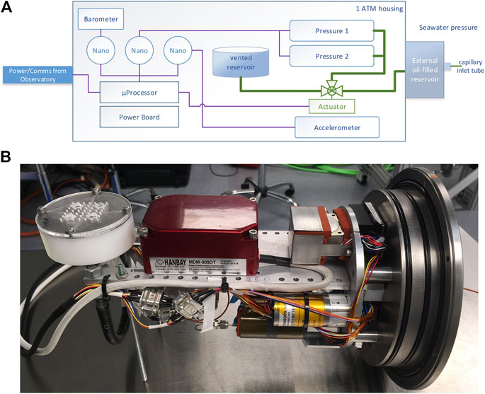
FIGURE 1. (A) Block diagram for the Geodetic and Seismic Sensor Module (GSSM). A pair of Paroscientific pressure sensors (model 42K-101) connect to an actuator-controlled, 3-way ball valve that toggles between external seawater pressure and internal housing pressure of ∼1 atm by sending commands from shore. The Paroscientific barometer (model 216B) provides an accurate reference measurement of internal housing pressure. A Quartz Seismic Sensors three-component accelerometer continuously monitors seafloor motion. Three Paroscientific Nano-Resolution electronics boards capture high resolution sensor measurements, timestamping them and passing them in real time to an onshore computer through the microprocessor. Thick green lines represent oil-filled plumbing. Thin purple lines represent data paths. (B) Photograph of the GSSM in the laboratory. The Paroscientific Seismic and Ocean Sensors module is on the right-hand side with the barometer on top, the accelerometer in the front on the bottom and one of the pressure sensors visible behind. The Hanbay valve actuator is in the center and the internal oil reservoir on the left. Reproduced from Wilcock et al. (2018).
As in the SCPR, the oil filled lines to the pressure sensor are connected to a 3-way Swagelok ball valve that is operated by a Hanbay motorized actuator to switch between the external ocean pressure and the internal pressure for the A-0-A calibrations. For this experiment, the oil used was Dow Corning FS-1265 flurosilicone fluid (300 centistoke-grade kinematic viscosity), which has a density of 1,250 kg m−3 and is thus denser than seawater. A small amount of oil leaks through the valve into the pressure case when the valve turns, so an external oil reservoir is included to prevent the ingress of seawater to the instrument plumbing, and an internal reservoir captures the oil within the instrument housing and avoids the potential effects of surface tension if the oil is allowed to drip from the internal tubing. Based on laboratory measurements that showed ∼4 cm3 of oil would leak through the valve for 100 turns at high pressure, the external reservoir was conservatively designed with a capacity of 40 cm3 for ∼1,000 valve cycles with the expectation that the number of calibrations would not exceed 200. The external oil reservoir is a cylindrical chamber machined in plexiglass with the axis oriented horizontally (Figure 2A). An outlet at the bottom connects to the plumbing in the pressure housing and an outlet at the top connects to the ocean via a short length of thin horizontal peek capillary tubing. As oil leaks through the valve, seawater replaces oil at the top of the chamber. The internal fluid reservoir is a simple cup with an internal diameter of 7 cm. The wide cross-sectional area was chosen to minimize the change in oil elevation that would occur during the deployment, but the design requires the instrument orientation to be maintained within ∼20° at all times during deployment to avoid oil spilling out.
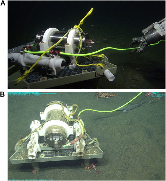
FIGURE 2. Photographs of the GSSM (A) The instrument during deployment with the external oil reservoir and inlet capillary tube visible on the right-hand side of the pressure housing. (B) The instrument just before recovery. There is no visible scouring of sediments around the platform legs.
The MARS cabled observatory operated by Monterey Bay Aquarium Research Institute (MBARI) provided power, communications to control the valve and retrieve the data, and precise one pulse per second timing. Custom electronics condition the incoming observatory power and custom software provide a user interface through which operators can control the internal valve and sensors in real time from shore. The GSSM was deployed at 36° 42.7481′N, 122° 11.2139′W at a depth of 887°m (Figure 3) on June 13, 2017 using the MBARI R/V Rachel Carson and ROV Ventana. For the deployment, the pressure housing was secured to a triangular grated platform, measuring ∼80 cm on each side (Figure 2). Three 5-cm-diameter hollow cylindrical legs made of fiberglass extended ∼30 cm beneath the platform and were designed to be driven into the soft muddy sediment to embed the instrument into the seafloor. The GSSM was attached to the junction box on the MARS cabled observatory with a 50-m-long Falmat power and ethernet cable with a wet-mate ODI connector. Data collection ended on December 14, 2019 and the instrument was recovered on December 17, 2019 by the same vessel and ROV. Prior to the recovery, the legs of the platform were inspected carefully, and no evidence of sediment scouring was observed (Figure 2B).
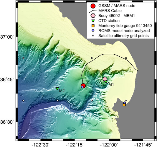
FIGURE 3. Bathymetric map of Monterey Bay showing the location of the MARS cable (black line) and main MARS node and GSSM (red circle). Also shown are the positions MBARI buoy MBM1 (NOAA buoy 46092) (pink hexagon), MBARI CTD sites Mooring one and Mooring 2 (inverted green triangles labeled M1 and M2), the NOAA Monterey tide gauge 9413450 (orange square), nodes in the ROMS model that are used to obtain pressure time series for comparison (purple circles) and grid points for the reprocessed multi-mission altimeter satellite sea surface heights (white diamonds).
The pressure sensors and accelerometer were sampled at 40 Hz and the barometer at 1 Hz. The low-pass filter implemented by the processing electronics was initially set to 0.5 Hz for the pressure and accelerometer data, but was increased to 8 Hz on August 25, 2017. The data were streamed to a laptop in the shore station and uploaded each day to the University of Washington for analysis and archiving. A total of 154 A-0-A calibrations were performed with each lasting 5 min. The calibrations were initially spaced 1 day apart. The interval then increased incrementally to two weeks over the first year of the deployment and was held at this value for the second year. For the first 10 calibrations, the valve actuator was only turned on for the calibration interval but subsequently it was left on permanently which resulted in an increase in the internal temperature of the housing. For the final six months of the deployment, the actuator was turned on only for valve turns which decreased the internal housing temperature again. During this last period, the calibration interval was reduced to one day and then increased to one week.
Oceanographic Data
In order to enable comparisons of long-term trends in the measured bottom pressures with those predicted from physical oceanographic data, we used two approaches to obtain time series of predicted bottom pressure. First, we obtained predicted bottom pressures by combining the sea surface height (SSH) anomalies determined from satellite altimetry data with a time series of repeat conductivity, temperature and depth (CTD) profiles that are collected by MBARI approximately monthly at two mooring stations M1 and M2, that lie 15 and 17 km to the east and west of the MARS observatory, respectively (Figure 3). The SSH anomaly was obtained from the Global Ocean Gridded L4 Sea Surface Heights and Derived Variables Reprocessed data set that is provided by the Copernicus Program (Taburet et al., 2019). Time series of daily SSH anomaly at stations M1 and M2 were obtained from the daily quarter degree spatial grids by linear interpolation for the period June 1, 2017 to October 15, 2019, the last date for which the reprocessed data were available at the time of analysis. The CTD casts were obtained from June 2017 to December 2019 and for each cast with good data that extended from ≤5 m to at least 500 m depth (36 casts at station M1 and 28 at station M2), a vertical profile of temperature and salinity to 900 m depth was created by combining the CTD casts from the surface to 500 m, with a seasonally-dependent temperature and salinity model from the 2018 World Ocean Atlas (Locarnini et al., 2018; Zweng et al., 2018) at greater depths. These profiles were converted to density using the Gibbs Seawater Oceanographic Toolbox (McDougall and Barker, 2011) and interpolated linearly with time to obtain daily profiles at stations M1 and M2 for each day in the altimetry time series. The density was then multiplied by the acceleration of gravity and integrated vertically to 887 m plus the SSH anomaly to estimate the pressure at the depth of the GSSM.
Second, we obtained predicted bottom pressures from the West Coast Ocean Forecast System (WCOFS) ocean circulation model developed at the National Oceanic and Atmospheric Administration (NOAA) Coast Survey Development Laboratory (Kurapov et al., 2017a; Kurapov et al., 2017b). The WCOFS model is constructed using the Regional Ocean Modeling System (ROMS) framework which utilizes the Boussinesq approximation and solves for hydrostatic pressures (Shchepetkin and McWilliams, 2005). The WCOFS model domain extends from 24° to 54°N along the North American coast and has 40 vertical layers with grid nodes spaced 2 km apart horizontally. This model was not developed to predict seafloor pressure but it was previously used for comparisons with seafloor pressure gauges off the coast of the Pacific Northwest (Fredrickson et al., 2019b) where it was shown to produce many of the statistical characteristics of the observed pressure field but not necessarily individual features. Modeled daily averaged pressures were calculated at the nodes closest to the GSSM and the Monterey tide gauge (Figure 3) from December 17, 2016 to November 14, 2018, the last date for which model output was available at the time of analysis. Tide height data from the Monterey tide gauge (NOAA station 9413450) was also downloaded and corrected for atmospheric pressure using barometric data from the MBARI buoy MBM1 (NOAA Station 46092) (Figure 3).
Results
Over the 914-days recording interval, the GSSM successfully collected data for all but 26 days with data gaps of up to 4 days resulting mostly from scheduled and unscheduled shutdowns of the observatory. Figure 4A shows power spectra for the accelerometer and pressure sensors for a typical day in the winter. The microseism peak is visible on all channels between 0.1 and 1 Hz. At lower frequencies spectral levels increase with decreasing frequency due to the effects of infragravity waves and noise levels are much higher on the horizontal accelerometer channels than the vertical accelerometer channel due to the effects of instrument tilting (Webb, 1998). At frequencies above the microseism peak, the spectral levels on the accelerometer channels increase above ∼3 Hz due to the increased frequency counting noise at higher frequencies and there is a pronounced peak at ∼8 Hz. Correcting the vertical channel for the tilt and compliance signals following the method of Crawford and Webb (2000) shows that this peak is a result of instrument tilting (Figure 4A) presumably due to a resonance with the seafloor. The relatively low noise floor of a few parts-per-billion of the full-scale range of 30 m/s2 near 1 Hz provides a useful band in which to record seismic events (Figures 4B,C).
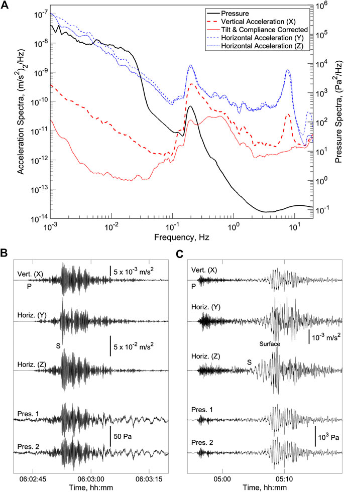
FIGURE 4. (A) Acceleration and pressure power spectra density for January 25, 2018 obtained using Welch’s method with 1-h windows, a Hamming taper, and 90% overlap. Spectral values have been smoothed by averaging samples with frequencies within ±10% of each sample. Correcting the vertical channel for compliance and tilt noise using the method of Crawford and Webb (2000) as implemented by Janiszewski et al. (2019), shows that the peak in accelerations at ∼8 Hz is a result of instrument tilting (B) Example record section showing 40 s of data for the accelerometer and pressure sensor for a magnitude 3.6 earthquake that occurred 53 km to the northeast of the GSSM near Aromas, California on January 24, 2018 with the P and S waves labeled. The vertical accelerometer is scaled by a factor of five relative to the horizontal channels and the pressure records have been filtered with a 0.2 Hz high pass filter. The S waves are dominated by energy at 0.5–1 Hz and the amplitudes are suppressed on the pressure sensors because the data is narrowband because it was acquired with a 0.5 Hz low pass filter. (C) Example record section showing 25 min of data for the magnitude 8.1 Chiapas, Mexico earthquake on September 7, 2017 with the P, S and surface waves labeled. A 0.005–2 Hz bandpass filter has been applied to all the data. There is a marked difference between the frequency of the P waves and the S and surface waves.
Figure 5A shows one day of pressure data from the first summer of the deployment. At this time, the external pressures on the two pressure sensors differ by ∼0.3 hPa, although by the end of the deployment they are several hPa apart. Over the day, the pressures vary by over 100 hPa due to diurnal and semi-diurnal tides but the difference between the two sensors remains stable within about ±0.05 hPa. The spectrum of the pressure difference (Figure 5B) shows an inverse dependence on frequency at frequencies below ∼0.5 Hz and have levels that are consistent with the predictions for electronic noise on the crystal oscillators of Webb and Nooner (2016). At frequencies above ∼1 Hz, the differences are quite small because the two sensors share the same counting electronics and the low pass filter was set to 0.5 Hz at this point in the experiment. Over shorter intervals (Figure 5A inset), the pressure sensors resolve the pressure excursions due to infragravity waves with periods of ∼100 s and microseisms with periods of about 5 s.
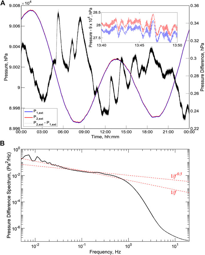
FIGURE 5. (A) Example day of external pressure data from July 2, 2017, a day without an A-0-A calibration. The two pressure sensors (blue and red lines and left axis) track each other over the tidal cycle within a range of ∼0.1 hPa (black line and right axis). (inset) Ten minutes of pressure with variations due to infragravity waves with periods of ∼100 s and microseisms with periods of <10 s. (B) Spectrum of the difference between the two pressure sensors (black lines) together with approximate f−1 and f−0.5 fits to the spectrum for frequencies below ∼0.5 Hz. Note that at this point in the development the low pass filter was set to 0.5 Hz for the pressure sensors.
At the onset of a calibration (Figure 6), it takes about 3 s to fully turn the valve with two-thirds of the pressure drop occurring over 0.5 s. The measured pressure drop initially overshoots to pressure lower than atmospheric because of short term viscoelastic transients and because the adiabatic expansion of oil leads to cooling that takes some time to equilibrate. During the calibration, the pressures recover approximately exponentially, and we chose to measure the calibration pressure by averaging pressures from each gauge and the barometer from 3 to 4 min after the pressure first decreases below 1,000 hPa near the end of valve turn. The offset of each external pressure gauge from the barometer is then recorded. It is important to obtain all calibration measurements over the same time interval relative to the time of the valve turn, but provided the calibration average is obtained starting at least 2 min after the turn and over at least 30 s, the consistency of the calibrations is not sensitive to when this is done. At the end of the calibration when the valve turns back, there is initially a small pressure drop related to the valve plumbing and the pressure then returns to its external value over a slightly longer time interval than observed for the value opening (just under half of the pressure increase occurs over 0.5 s). The effect of the calibration is to temporarily perturb the external pressure toward slightly lower values. Measured pressures are ∼0.5 hPa too low 30 s after the calibration, but they essentially recover over about 10 min.
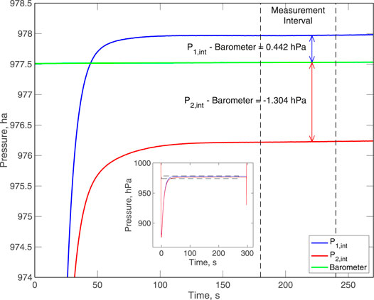
FIGURE 6. Pressure data for an example calibration, showing all but the first and last 30 s. The calibration is obtained by averaging the pressure measurements between 180 and 240 s after the onset of the test and measuring the offset of the pressure gauges from the barometer. (inset) Pressure data for the full 5-min calibration. Initially the pressures undershoot but they then recover approximately exponentially on a timescale of ∼20 s. Reproduced from Wilcock et al. (2018).
The first calibration was obtained within minutes of attachment to the MARS cabled observatory to test the valve commands while the ROV was still nearby; the results are not reliable because the GSSM had not reached thermal equilibrium with its surroundings. The remaining 153 are plotted in Figure 7A along with the temperature measured by one of the pressure gauges (the pressure gauge temperatures are offset from each other by ∼0.06°C but are consistent with each other to ∼0.002°C). For both sensors the changes in temperature which accompany changes in the valve actuator operation, result in a clear jump in measured offset. Over the course of the experiment the offset measured for the first pressure sensor increases by over 6 hPa while the offset on the second pressure sensors increases by nearly 2 hPa. Thus, the pre-calibration drift rates of the two pressure sensors was significantly better than the ∼1 part in 104 per year (or ∼10 hPa in 1,000 m of water) reported for some sensors (Polster et al., 2009).
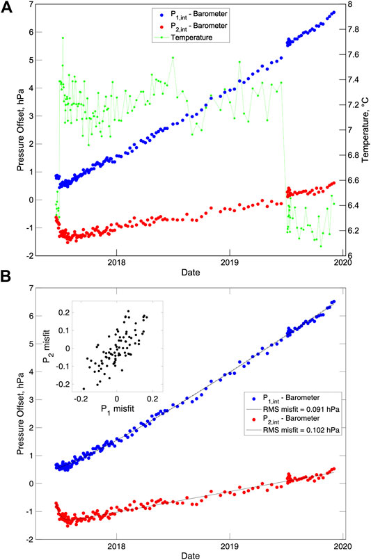
FIGURE 7. (A) Pressure offsets (pressure gauge minus barometer) measured during the calibrations for the two pressure gauges (blue and red circles) and temperature measured inside the pressure housing by the second pressure sensor (green points connected by a thin line). The temperature increased by ∼0.8°C early in the deployment when the operation of the valve actuator was changed from turning on the power just for the 5-min calibration to leaving it on permanently. The temperatures decreased by ∼0.9°C for the last 6 months when the valve actuator was only turned on for the valve turns at the start and end of the calibration. (B) Pressure offsets after applying a linear temperature correction (see text) with smooth fits to the data (black lines). (inset) Plot of the misfits of the calibrated pressure offsets from the smooth curve for the two sensors showing that they are strongly correlated.
The drift of the Paroscientific pressure sensors can be explained as the sum of two exponential terms of opposite sign (Paros and Kobayashi, 2015b). Outgassing from the quartz crystal causes drift to higher frequencies and pressures and has a long time constant. On shorter time scales, viscoelastic creep of the quartz crystal attachments in response to the pressure history of the crystal causes drift to lower frequencies and pressures. A number of mathematical models can be used to fit the drift of Paroscientific sensors (Paros and Kobayashi, 2015a). Here, we find it adequate to follow the approach of several previous studies (Chiswell and Lukas, 1989; Watts and Kontoyiannis, 1990; Polster et al., 2009; Kajikawa and Kobata, 2019) with the addition of a temperature dependent term, and fit a function of the form
where p(t) is the pressure offset as a function of time since the deployment, T is the temperature relative to a reference temperature Tref that is set to the median of the deployment and a, t0, b, c and d are constants. The exponential term accounts for viscoelastic creep that is observed when ambient pressure changes and the linear term is sufficient to model the effects of outgassing on the timescale of our experiment. We use a least squares linear inversion to solve for a, b, c and d for different fixed values of the exponential time constant t0 and select the value of t0 that gives the minimum root mean squared (RMS) residual. Figure 7B shows the temperature corrected offsets together with a smooth curve obtained for the remaining terms in Eq. 1. For pressure sensors 1 and 2, the best fitting curves have an exponential time constant of 280 and 14 days and yield an RMS misfit of 0.091 and 0.102 hPa, respectively. The early measurements for pressure sensor two are fit better if a second exponential term with a time constant of 9 days is added, which reduces the RMS residual to 0.087 hPa. Inspection of the residuals obtained from subtracting the modeled offsets from the observations, shows that they are strongly correlated between the two sensors (correlation coefficient = 0.83).
If the sensitivity or span of a pressure sensor remined constant, then the difference between repeat measurements of a fixed high and a fixed low pressure should be invariant with time. This cannot be tested with the field observations on a single sensor by comparing the pre-calibration external pressure with the internal calibration pressure. This is because the pressures are not fixed primarily because the external pressure changes with tides and other oceanographic effects. However, if the difference between the external and internal pressure is compared between two sensors, the difference should not change with time if the sensitivities of both sensors are constant. In order to assess the consistency of the calibrations between sensors, we calculate the span of the two instruments by subtracting the pressure measured during the calibration from the external pressure averaged from 65 to 5 s before the start of the calibration and then look at the difference of the two spans. After applying a linear temperature correction, the results (Figure 8A) show that the two sensors remain consistent with each other within just over 0.2 hPa for the 30-month deployment. After the first two months of the deployment, the two sensors drift apart approximately linearly at a rate that averages 0.08 hPa/yr. The A-0-A calibrations improve the self-consistency of the two pressure measurements by well over an order of magnitude (Figure 8B) and the relative drift rates of one part in 106 are two orders of magnitude better than the typical drift rates of uncalibrated sensors reported by Polster et al. (2009).
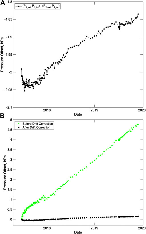
FIGURE 8. (A) Difference in span between the two pressure sensors after applying a linear temperature correction. The span for each sensor is measured by subtracting the internal pressure measured during a calibration from the external pressure averaged for a minute just before the calibration. (B) Change in offset of the external pressures between the two sensors at the times of calibrations relative to the time of the first calibration shown before (green triangles) and after (black circles) applying the drift correction.
Discussion
Applying the Pressure Calibrations
Several small corrections need to be applied to the A-0-A calibrations. Upon recovery the oil level in the external reservoir was found to have dropped by about 0.6 cm which would lead to an apparent decrease in the measured external pressures of 0.13 hPa as seawater replaced the denser oil. The measured drop requires that 8 cm3 of oil leaked through the valve which is reasonably consistent with the prediction of 6 cm3 obtained from laboratory testing of the valve. The oil levels in the internal reservoir are estimated to have risen by 0.2 cm. While this was not accurately measured, it was noted that the oil level in the internal reservoir changed only slightly. A 0.2 cm increase in the internal reservoir oil level would increase the internal pressure measurements by 0.25 hPa, and thus reduce the calibrated external pressures by the same amount. The net effect of the changes in levels in the two reservoirs is corrected by increasing the observed change in external pressures over the deployment by 0.38 hPa.
After the experiment, the frequency of the counting clock used to measure the frequency of the temperature and pressure sensing crystals in the pressure gauges was found to have drifted over the 30-months deployment to higher frequencies by a fraction of 1.05 × 10⁻⁶. The equivalent annual rate of 0.42 × 10⁻⁶, is consistent with Sasagawa et al. (2018) who reported that the fractional frequency drift for 12 systems averaged 0.2 × 10⁻⁶ yr−1 and never exceeded 0.5 × 10⁻⁶ yr−1. Using the equations presented in the manual for the counting electronics to convert frequency to temperature and pressure (Paroscientific, Inc., 2016), the resulting drift for pressure sensor one is calculated as 1.12 hPa at the external pressure of 900 MPa and 0.95 hPa for the internal pressure of 10 MPa. For the pressure 2, the corresponding values are 1.17 and 0.99 hPa. Since the A-0-A calibrations correct for the drift at internal pressures, the remaining effect of counting clock drift on external pressure is corrected by decreasing the observed change in external pressures over the deployment by 0.17 and 0.18 hPa, respectively.
Any drift of the barometer will also offset the calibrations. The Paroscientific 216B barometer is certified to drift at less than 0.01% (0.1 hPa) per year but typically drifts at about a 10th this rate. We have not recalibrated the barometer because we anticipate this to be a very small correction. For a less stable barometer, it would be important to do this.
The pressure measurements are dependent on the stability of the instrument platform. Figures 9A and 9B shows the smoothed change in tilt over the deployment measured using the two horizontal accelerometer channels (Figure 10 shows the channel orientations relative to the instrument platform). The tilt rates of several milliradians per year are equivalent to about one part in 103 of the ±3 g measurement span and thus significantly exceed the expected drift of the accelerometer at no more than one part in 104. We verified the reliability of the horizontal tilts by computing the resulting change in total tilt of the platform and comparing it to an equivalent calculation from the vertical accelerometer after applying a correction for its drift determined from the change in magnitude of the total vector acceleration which, in the absence of sensor drift, should be constant (Fredrickson et al., 2019a). The results of comparison (Figure 1C) show that the two measurements are consistent within <0.04 mrad, confirming that the horizontal tilts are reliable. Paroscientific pressure gauges are sensitive to orientation because the pressure sensing crystal cannot be fully isolated from the effects of gravitational loading. In the Paroscientific SOS module, these corrections are automatically applied based on the output of the horizontal tilt sensors and were <0.1 hPa for the observed tilts in our experiment.
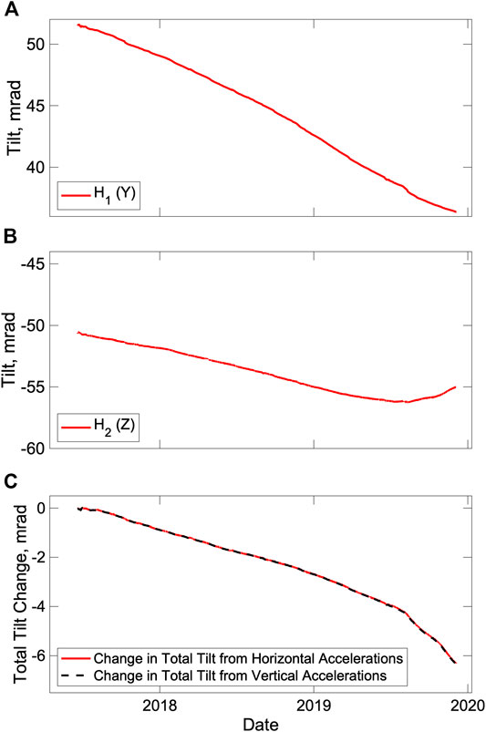
FIGURE 9. Tilt measured by the accelerometer from June 20, 2017 to the end of the deployment after applying a 1 day running mean. (A) Tilt on the horizontal channel Y. (B) Tilt on the horizontal channel Z. (C) Change in total tilt relative to July 1, 2017. This was calculated from combining the horizontal tilts using the small angle approximation and from the change in vertical acceleration after correcting for the sensor drift and the resulting curves are identical at the scale of the plot.
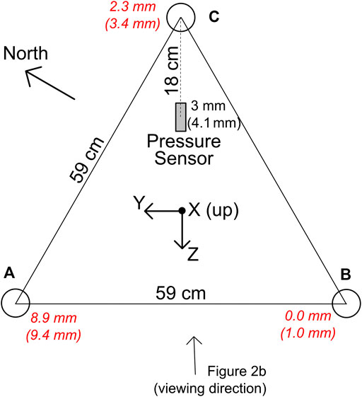
FIGURE 10. Schematic showing the approximate relative locations of the instrument legs and the pressure sensors and the orientation of the accelerometer channels. The convention for the accelerometer is that accelerations are positive when their point away from the channel orientation so that the X channel which points up records the acceleration of gravity as a positive number. The orientation of the instrument is such that the Z-axis is at an azimuth of ∼240° with respect to north. Labels in red italics on the sensor legs and pressure sensor give estimates of the subsidence of those components based on summing the minimum subsidence for two intervals between which the rate of change of the Z channel tilt changed sign, with a second estimate based on summing daily calculations shown in parentheses (see text).
The tilting of the platform is most simply explained by platform subsidence which can be expected to be most significant in settings such the MARS observatory where the instrument is deployed on soft mud. Accounting for platform subsidence is a significant challenge in seafloor geodesy (Cook and DeSanto, 2019). We can estimate a minimum subsidence from the tilt measurements under the assumption that at any instant, not all legs are subsiding, and no legs are rising. If we ignore the first two weeks of data in June when the tilt data suggests the platform was settling unevenly and divide the tilt time series in two for this calculation at the time where the sign of the rate of change of tilt on the horizontal Z channel changed (Figure 9B), we estimate that the pressure sensor subsided by 3.0 mm, equivalent to an apparent pressure increase of 0.3 hPa (Figure 10). Performing this calculation on daily changes in smoothed tilt, predicts 4.1 mm of subsidence. In both cases most of the observed tilt can be modeled as the result of subsidence of one leg by nearly 1 cm (Figure 10). Performing the calculations on shorter intervals with unsmoothed data leads to higher subsidence predictions but these are likely to be unreliable given that tides and tidal currents can be expected to rock the platform back and forth on timescales of a day or less without necessarily leading to subsidence. Of course, the pressure sensor may have subsided more than calculated if all the legs subsided together, and ideally an independent means should be employed to measure this in sedimented settings (Cook and DeSanto, 2019). To account for subsidence, we chose to reduce the observed changes in external pressure over the experiment by 0.3 hPa, since this is the minimum feasible correction.
Figure 11 shows the detided external pressure data after applying the calibration curves of Figure 7B with an additional correction that reduces the change in pressures over the deployment by 0.1 hPa to account for the combined effects of changes in oil reservoir levels, counting clock drift and the minimum subsidence. The two calibrated pressure sensors track each other very closely, showing an apparent tendency for higher pressures in the summer than winter. There is an apparent slope in pressure over the course of the experiment of 0.48 and 0.43 hPa/yr for the two pressure sensors, respectively.
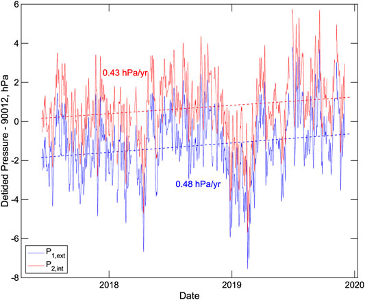
FIGURE 11. External pressures measured by the two pressure sensors after removing tides using a low-pass Godin filter comprising successive running averages of 24, 24, and 25 h (Godin, 1972) and applying drift corrections based on the calibration curves of Figure 7B with an additional small correction for the combined effects of changes in the reservoir heights, counting clock drift and the minimum platform subsidence required to explain tilt changes of the instrument (see text).
Comparisons With Oceanographic Predictions
Because Monterey Bay is not situated in a region that is prone to vertical tectonics and the MARS observatory is located in an area with muted bathymetry that is not subject to slope instability, the measured trends of increasing pressure over the experiment must be due to oceanographic processes if they are not the result of additional platform subsidence or an unidentified systematic measurement error.
Figure 12 shows a comparison between the calibrated GSSM pressure time series and the pressures predicted at station M2 at 887 m depth by combining the SSH anomalies and time dependent water column density structure. Station M2 which lies to the west of the GSSM (Figure 3) was selected because it is a site of monthly CTD casts. The incorporation of the water column density structure into the pressure predictions substantially modulates the pressure variations predicted from SSH anomalies alone (blue dashed line in Figure 12), reducing the overall amplitude of variations, as would be expected given that the component of sea surface height anomalies associated with currents that do not extend to the depth of the GSSM will be compensated by density variations at depth. The predicted pressure variations are generally similar to the calibrated GSSM pressure variations showing many of the same long-period features. Only in a few instances do the curves deviate from one another during an interval when there are constraints on density from a CTD cast. Over the interval for which there is reprocessed satellite altimetry, which is all but the last two months of the GSSM deployment, the observed and predicted time series show trends in increasing pressures (0.4 hPa/yr for the pressure sensor two and 0.5 hPa/yr for the altimetry and CTD predictions) that are remarkably consistent.
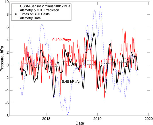
FIGURE 12. Comparison of GSSM pressure with the bottom pressures predicted at station M2, 17 km to the west using satellite altimetry and repeat CTD casts. Calibrated detided pressure for GSSM pressure sensor 2 (red line) are compared to the pressures obtained from the altimetry data and water column density profiles (bold black line with solid circles showing the time of CTD casts) and those predicted directly from altimetry data (dashed blue line). A least squares straight lie fit labeled with the slope is shown for the first two curves (dashed lines).
Efforts to derive predicted bottom pressures at station M1, a second site with monthly CTD casts, were less successful. Here the interpolated satellite sea surface height anomalies are smaller than at station M2, and the water column density structure overcompensates many features leading to bottom pressure variations with higher amplitudes than those predicted from the satellite altimetry alone. We infer that the interpolated altimetry data are unreliable and muted at site M1 because it includes a contribution from grid points that are very close to the shore (Figure 3) (Cipollini et al., 2017).
Figure 13 shows comparison of the pressure predictions of the ROMS model with the Monterey tide gauge and the calibrated GSSM pressures. The ROMS model matches the seasonal variations in the pressures obtained from the Monterey tide gauge quite well (Figure 13A). Lower pressures are observed in the spring and early summer as is typically observed at the coast in this region (Ryan and Noble, 2002), and over the 30-months interval of the GSSM data, the tide gauge shows a trend in increasing pressures of 1.1 hPa/yr.
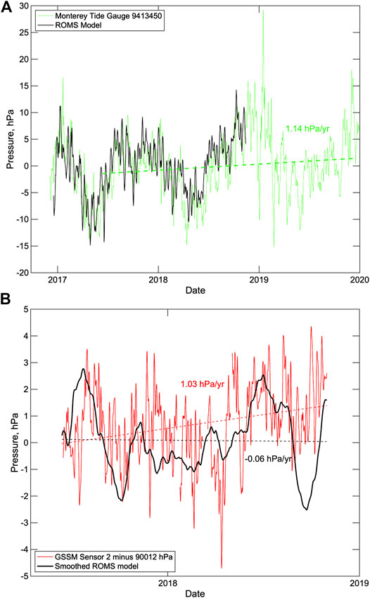
FIGURE 13. Comparisons of observed pressures with the predictions of a ROMS circulation model (Kurapov et al., 2017a; Kurapov et al., 2017b). (A) Tide gauge record from Monterey (station 9413450) converted to pressure and adjusted for atmospheric pressure (green line) compared to the ROMS model at a node 1 km to the north at 10 m depth (black line). The seasonal variations and trends in the tide gauge data are well matched for the period December 17, 2016 to November 14, 2018. A least squares straight line fit (dashed line) labeled with the slope is shown for the tide gauge data for June 13, 2017 to December 14, 2019 (the interval of operation of the GSSM). (B) Calibrated, detided pressure for GSSM pressure sensor 2 (red line) compared with the ROMS model at a node 0.8 km to the southwest at a depth of 1,083 m (black line) for the period June 13, 2017 to November 14, 2018. A 29-days running mean has been applied to the ROMS model because the average daily solutions display a strong residual spring-neap tide signal that is only apparent in deeper waters. A least squares straight line fit (dashed line) labeled with the slope is shown for each time series.
For the GSSM comparison (Figure 13B), the ROMS model has been smoothed with a 29-days running mean to remove a strong residual spring-neap tide signal with a period of 14–15 days. The comparison is limited to 16½ months from the start of the GSSM deployment and the trends obtained with a least squares linear fit are not well matched, with the GSSM data showing a slope of 1 hPa/yr and the ROMS model slope near zero. This mismatch is almost entirely a result of a large trough in predicted pressures in ROMS model in late summer and fall 2018 that is not present in the GSSM pressures. Over the first 14 months, the predictions and observations are in much better agreement and the slopes of a linear fit are similar. As Fredrickson et al. (2019b) notes, the WCOFS ROMS model predicts pressure better near the coast than in deeper water because it is primarily validated with observations from the continental shelf, and the processes that influence density structure in the deeper ocean are less deterministic. Furthermore, the bathymetry in the vicinity of the GSSM is complex because of the presence of the Monterey Canyon and the local effects of this bathymetry on circulation will not be fully simulated in a regional model with limited spatial resolution. A longer time series would be required to adequately compare the long-term trends in bottom pressure with those predicted by the ROMS circulation model.
The trend of increasing pressure seen in our data are consistent with the trend expected from the El Niño Southern Oscillation. Data from the San Francisco tide gauge show that during the winter months, sea surface heights at the coast are about 4 cm higher during El Niño and 4–5 cm lower during La Niña (Ryan and Noble, 2002). This effect is not a result of density structure but is related partly to variations in local wind stress moving water toward or away from the coast and partly due to the effects of coast trapped waves generated by wind stresses elsewhere (Ryan and Noble, 2002). The first winter of the GSSM deployment coincided with a weak La Niña event from October 2017–March 2018 while the latter parts of the deployment coincided with weak El Niño conditions from October 2018–June 2019 and November–December 2019. Thus, average sea surface heights, and by inference bottom pressure, would be expected to increase during the deployment.
Precision and Accuracy of the Calibrated Pressures
The remarkable agreement between the calibrations on the two sensors is consistent with a precision in correcting drift of 0.1 hPa/yr or one part in 106, but experiments with more sensors will be required to demonstrate that this can be achieved consistently. Because the discrepancy between the sensors is so small and there is possibly an unknown component of subsidence that was not measured by the tilt meter, it is not possible to determine whether the accuracy of the drift removal matches the precision. However, given that the observed trend in pressure of only 0.5 hPa/yr closely matches that calculated from satellite altimetry and repeat CTD casts at a nearby location, and that the sign of the trend agrees with that expected for the El Niño Southern Oscillation, it is very likely that the calibrations are accurate to much better than one part in 105.
The drift rates observed on Paroscientific sensors are proportional to the depth rating (Paros and Kobayashi, 2015b) so the precision observed in the GSSM experiment with 1,400 m (2000 psi) sensor would equate to a 0.5 hPa/yr for a 7,000 m (10,000 psi) full ocean depth sensor. In subduction zones, the signals from slow slip events observed to date have amplitudes of several centimeters and so may lead to resolvable permanent offsets in bottom pressure when observed with A-0-A calibrated pressure gauges. For secular strain, the magnitude of the expected signals is ≤1 hPa/yr (Fredrickson et al., 2019b) so here A-0-A calibrated pressure gauges are more likely to be successful in resolving strain when they are deployed at relatively shallow depths with the appropriate depth-rated sensors. Resolving geodetic signals will, off course, also require paying careful attention to removing oceanographic signals that also limit the resolution of seafloor pressure measurements for geodesy.
Conclusion
A 30-month test of the A-0-A technique for calibrating seafloor pressure gauges at 900 m in Monterey Bay, resulted in calibrated pressure records on two Paroscientific pressure gauges that are consistent with each other to one part in 106 per year, well over an order of magnitude improvement relative to the uncalibrated pressure gauges. The calibrated pressure gauges detected an overall trend in increasing seafloor pressure of ∼0.5 hPa/yr which matches well with that predicted by combining sea surface height anomalies from satellite altimetry with CTD data at a site 17 km seaward of the test site. The trend is qualitatively consistent with the pattern expected based on sea level variations due to the El Niño Southern Oscillation. However, because there is an unknown component of platform subsidence and the deployment interval was short compared with that necessary to resolve oceanographic trends, the absolute error of the calibrations is not fully constrained.
For applications where a pressure gauge drift of one part in 105 is sufficiently small to resolve the signals of interest, our seafloor experiment and the laboratory tests of Sasagawa et al. (2018) show that A-0-A calibration is more than sufficient. For applications where a drift approaching one part in 106 is required, additional experiments are required to fully evaluate the A-0-A method. These will require long multi-year deployments in stable well-characterized settings and careful attention to characterizing platform stability and subsidence. The results should be compared with those obtained from other methods of pressure gauge drift removal and ideally with the pressure variations predicted from physical oceanographic observations.
Data Availability Statement
The datasets presented in this study can be found in online repositories. The names of the repository/repositories and accession number(s) can be found below: The data collected by the GSSM has been archived at the University of Washington in the Research Works database and is available at http://hdl.handle.net/1773/46596 (Wilcock et al., 2020).
Author Contributions
WW interacted closely with the engineering team, undertook the data analysis and wrote the manuscript. DAM was the project manager leading the engineering design, fabrication and testing of the GSSM and directed the deployment and recovery of the instrument at sea. EF contributed to the comparisons with oceanographic data. MH, GC, JT, JB, and DeM participated in the design, fabrication and testing of the GSSM. TK demonstrated how to analyze the accelerometer data for sensor tilt. JP proposed the A-0-A approach for calibrating seafloor pressure gauges and provided advice on the GSSM design and data analysis.
Funding
This work was supported by JP, the Jerome M. Paros Endowed Chair in Sensor Networks, and the University of Washington.
Conflict of Interest
JP is the Founder, President and Chairman of Paroscientific, Inc., that develops and manufactures the quartz crystal sensors and the SOS module. He provided advice and support for the design of the GSSM and the best approaches for correcting sensor drift but was not directly involved in the acquisition or analysis of the data.
The remaining authors declare that the research was conducted in the absence of any commercial or financial relationships that could be construed as a potential conflict of interest.
Acknowledgments
We thank the engineers at Paroscientific for support with the design and fabrication of the GSSM; the captain and crew of the R/V Rachel Carson and the operators of the ROV Ventana for their assistance deploying and recovering the GSSM; Craig Dawes for help connecting and operating the GSSM on the MARS cabled observatory; Francisco Chavez and Reiko Michisaki for providing access to the MBARI CTD data; Alex Kuparov for sharing the WCOFS regional oceanographic model simulations; Susan Hautala and Parker MacCready for helpful advice and assistance with the oceanographic data analysis; and Yoshichio Ito and Spahr Webb for thoughtful reviews.
References
Araki, E., Machida, Y., Nishida, S., Kimura, T., Yokobiki, T., and Kodaira, S. (2019). Seafloor pressure measurement to evaluate inter-plate coupling in the Nankai trough seismogenic zone. Available at: https://agu.confex.com/agu/fm19/meetingapp.cgi/Paper/513896 (Accessed August 1, 2020).
Blum, J. A., Chadwell, C. D., Driscoll, N., and Zumberge, M. A. (2010). Assessing slope stability in the Santa Barbara Basin, California, using seafloor geodesy and CHIRP seismic data. Geophys. Res. Lett. 37, L13308. doi:10.1029/2010GL043293
Bürgmann, R., and Chadwell, D. (2014). Seafloor geodesy. Annu. Rev. Earth Planet Sci. 42, 509–534. doi:10.1146/annurev-earth-060313-054953
Bürgmann, R., and Thatcher, W. (2013). Space geodesy: a revolution in crustal deformation measurements of tectonic processes. Spec. Pap. Geol. Soc. Am. 500, 397–430. doi:10.1130/2013.2500(12)
Chadwell, C. D., Hildebrand, J. A., Spiess, F. N., Morton, J. L., Normark, W. R., and Reiss, C. A. (1999). No spreading across the Southern Juan de Fuca Ridge axial cleft during 1994–1996. Geophys. Res. Lett. 26, 2525–2528. doi:10.1029/1999GL900570
Chadwick, W. W., Nooner, S. L., Butterfield, D. A., and Lilley, M. D. (2012). Seafloor deformation and forecasts of the April 2011 eruption at axial seamount. Nat. Geosci. 5, 474–477. doi:10.1038/ngeo1464
Chadwick, W. W., Nooner, S. L., Zumberge, M. A., Embley, R. W., and Fox, C. G. (2006). Vertical deformation monitoring at Axial Seamount since its 1998 eruption using deep-sea pressure sensors. J. Volcanol. Geoth. Res. 150, 313–327. doi:10.1016/j.jvolgeores.2005.07.006
Chiswell, S. M., and Lukas, R. (1989). The low-frequency drift of paroscientific pressure transducers. J. Atmos. Ocean. Technol. 6, 389–395. doi:10.1175/1520-0426(1989)006<0389:TLFDOP>2.0.CO;2
Cipollini, P., Calafat, F. M., Jevrejeva, S., Melet, A., and Prandi, P. (2017). Monitoring sea level in the coastal zone with satellite altimetry and tide gauges. Surv. Geophys. 38, 33–57. doi:10.1007/s10712-016-9392-0
Cook, M. J., and DeSanto, J. B. (2019). Validation of geodetic seafloor benchmark stability using structure-from-motion and seafloor pressure data. Earth and Space Science 6, 1781–1786. doi:10.1029/2019EA000623
Cook, M. J., Sasagawa, G., Roland, E. C., Schmidt, D. A., Wilcock, W. S. D., and Zumberge, M. A. (2017). “Campaign-style measurements of vertical seafloor deformation in the Cascadia subduction zone using and absolute self-calibrating pressure recorder,” in Fall Meeting 2017, New Orleans, LA, December 2017 [abstract].
Crawford, W. C., and Webb, S. C. (2000). Identifying and removing tilt noise from low-frequency (<0.1 Hz) seafloor vertical seismic data. Bull. Seismol. Soc. Am. 90, 952–963.
Davis, E. E., Villinger, H., and Sun, T. (2015). Slow and delayed deformation and uplift of the outermost subduction prism following ETS and seismogenic slip events beneath Nicoya Peninsula, Costa Rica. Earth Planet Sci. Lett. 410, 117–127. doi:10.1016/j.epsl.2014.11.015
DeSanto, J. B., and Sandwell, D. T. (2019). Meter-scale seafloor geodetic measurements obtained from repeated multibeam sidescan surveys. Mar. Geodes. 42, 491–506. doi:10.1080/01490419.2019.1661887
Doglioni, C., and Riguzzi, F. (2018). The space geodesy revolution for plate tectonics and earthquake studies. Rendiconti Lincei. Sci. Fis. Nat. 29, 29–34. doi:10.1007/s12210-017-0639-6
Fox, C. G. (1990). Evidence of active ground deformation on the mid‐ocean ridge: axial seamount, juan de Fuca ridge, April‐June 1988. J. Geophys. Res. Solid Earth 95, 12813–12822. doi:10.1029/JB095iB08p12813
Fox, C. G. (1993). Five years of ground deformation monitoring on axial seamount using a bottom pressure recorder. Geophys. Res. Lett. 20, 1859–1862. doi:10.1029/93GL01216
Fox, C. G. (1999). In situ ground deformation measurements from the summit of Axial Volcano during the 1998 volcanic episode. Geophys. Res. Lett. 26, 3437–3440. doi:10.1029/1999GL900491
Fredrickson, E. K., Wilcock, W. S. D., Baillard, C., Harrington, M., Cram, G., Tilley, J., et al. (2019a). “Observing and interpreting seafloor tilt at axial seamount,” in Fall Meeting 2019, San Francisco, CA, December 2019 [abstract].
Fredrickson, E. K., Wilcock, W. S. D., Schmidt, D. A., MacCready, P., Roland, E., Kurapov, A. L., et al. (2019b). Optimizing sensor configurations for the detection of slow-slip earthquakes in seafloor pressure records, using the cascadia subduction zone as a case study. J. Geophys. Res.: Solid Earth 124, 13504–13531. doi:10.1029/2019JB018053
Fujimoto, H. (2014). Seafloor geodetic approaches to subduction zone thrust earthquakes. Monogr. Environ. Earth Planets 2, 23–63. doi:10.5047/meep.2014.00202.0023
Inazu, D., Hino, R., and Fujimoto, H. (2012). A global barotropic ocean model driven by synoptic atmospheric disturbances for detecting seafloor vertical displacements from in situ ocean bottom pressure measurements. Mar. Geophys. Res. 33, 127–148. doi:10.1007/s11001-012-9151-7
Ito, Y., Hino, R., Kido, M., Fujimoto, H., Osada, Y., Inazu, D., et al. (2013). Episodic slow slip events in the Japan subduction zone before the 2011 Tohoku-Oki earthquake. Tectonophysics 600, 14–26. doi:10.1016/j.tecto.2012.08.022
Janiszewski, H. A., Gaherty, J. B., Abers, G. A., Gao, H., and Eilon, Z. C. (2019). Amphibious surface-wave phase-velocity measurements of the Cascadia subduction zone. Geophys. J. Int. 217, 1929–1948. doi:10.1093/gji/ggz051
Kajikawa, H., and Kobata, T. (2019). Evaluation and correction for long-term drift of hydraulic pressure gauges monitoring stable and constant pressures. Measurement 134, 33–39. doi:10.1016/j.measurement.2018.10.051
Kajikawa, H., and Kobata, T. (2016). Pressure gauge calibration applying 0-A-0 pressurization to reference gauge. Acta IMEKO. 5, 59. doi:10.21014/acta_imeko.v5i1.3192012
Kajikawa, H., and Kobata, T. (2014). Reproducibility of calibration results by 0-A-0 pressurization procedures for hydraulic pressure transducers. Meas. Sci. Technol. 25, 015008. doi:10.1088/0957-0233/25/1/015008
Kurapov, A. L., Erofeeva, S. Y., and Myers, E. (2017a). Coastal sea level variability in the US West Coast Ocean Forecast system (WCOFS). Ocean Dynam. 67, 23–36. doi:10.1007/s10236-016-1013-4
Kurapov, A. L., Pelland, N. A., and Rudnick, D. L. (2017b). Seasonal and interannual variability in along-slope oceanic properties off the US West Coast: inferences from a high-resolution regional model. J. Geophys. Res.: Oceans 122, 5237–5259. doi:10.1002/2017JC012721
Locarnini, R. A., Mishinov, A. V., Baranova, O. K., Boyer, T. P., Zweng, M. M., Garcia, H. E., et al. (2018). “Temperature,” in World Ocean Atlas 2018. Editor A. Mishonov (Boston, MA: U.S. Government Printing Office), Vol. 1, 52.
Matsumoto, H., Araki, E., Kawaguchi, K., Nishida, S., and Kaneda, Y. (2014). “Long-term features of quartz pressure gauges inferred from experimental and in-situ observations,” in OCEANS 2014–TAIPEI, Taipei, Taiwan, April 7–10, 2014 (Piscataway, NJ: IEEE), 1–4. doi:10.1109/OCEANS-TAIPEI.2014.6964447
McDougall, T. J., and Barker, P. M. (2011). Getting started with TEOS-‐10 and the gibbs seawater (GSW) oceanographic toolbox. SCOR/IAPSO. Technical Paper WG127.
McGuire, J. J., and Collins, J. A. (2013). Millimeter-level precision in a seafloor geodesy experiment at the Discovery transform fault, East Pacific Rise. Geochem. Geophys. Geosyst. 14, 4392–4402. doi:10.1002/ggge.20225
Muramoto, T., Ito, Y., Inazu, D., Wallace, L. M., Hino, R., Suzuki, S., et al. (2019). Seafloor crustal deformation on ocean bottom pressure records with nontidal variability corrections: application to hikurangi margin, New Zealand. Geophys. Res. Lett. 46, 303–310. doi:10.1029/2018GL080830
Nishida, S., Kimura, T., Machida, Y., and Araki, E. (2019). “Level adjust unit at seafloor for precise pressure measurement,” in 2019 IEEE Underwater Technology (UT), Taiwan, Taiwan, April 16–19, 2019 (Piscataway, NJ: IEEE), 1–4. doi:10.1109/UT.2019.8734331
Nooner, S. L., and Chadwick, W. W. (2016). Inflation-predictable behavior and co-eruption deformation at Axial Seamount. Science 354, 1399. doi:10.1126/science.aah4666
Nooner, S. L., Webb, S. C., Buck, W. R., and Cormier, M.-H. (2014). Post eruption inflation of the east Pacific rise at 9°50′ N. Geochem. Geophys. Geosyst. 15, 2676–2688. doi:10.1002/2014GC005389
Paros, J., Migliacio, P., and Schaad, T. (2012a). “Nano-resolution sensors for disaster warning systems,” in 2012 Oceans–Yeosu, Yeosu, South Korea, May 21–24, 2012 (Piscataway, NJ: IEEE), 1–5. doi:10.1109/OCEANS-Yeosu.2012.6263413
Paros, J., Migliacio, P., Schaad, T., Chadwick, W., Meinig, C., Spillane, M., et al. (2012b). “Nano-resolution technology demonstrates promise for improved local tsunami warnings on the MARS project,” in 2012 Oceans–Yeosu, Yeosu, South Korea, May 21–24, 2012 (Piscataway, NJ: IEEE), 1–6. doi:10.1109/OCEANS-Yeosu.2012.6263411
Paros, J. M., and Kobayashi, T. (2015a). Mathematical models of quartz sensor stability. Available at: http://paroscientific.com/pdf/G8095_Mathematical_Models.pdf.
Paros, J. M., and Kobayashi, T. (2015b). Root causes of quartz sensor drift. Available at: http://paroscientific.com/pdf/G8101_Root_Causes_of_Quartz_Sensors_Drift.pdf.
Paroscientific, Inc. (2016). Digiquartz broadband intelligent instruments with RS-232 and RS-485 interfaces: user manual. Available at: http://paroscientific.com/pdf/8819-001_Digiquartz_Operations_Manual_for_RS_485_RS_232_Products_715_Display.pdf.
Polster, A., Fabian, M., and Villinger, H. (2009). Effective resolution and drift of Paroscientific pressure sensors derived from long-term seafloor measurements. Geochem. Geophys. Geosyst. 10, Q08008. doi:10.1029/2009GC002532
Ryan, H. F., and Noble, M. (2002). Sea level response to ENSO along the central California coast: how the 1997–1998 event compares with the historic record. Prog. Oceanogr. 54, 149–169. doi:10.1016/S0079-6611(02)00047-2
Sasagawa, G., Cook, M. J., and Zumberge, M. A. (2016). Drift-corrected seafloor pressure observations of vertical deformation at Axial Seamount 2013–2014. Earth Space Sci. 3, 2016EA000190. doi:10.1002/2016EA000190
Sasagawa, G. S., Zumberge, M. A., and Cook, M. J. (2018). Laboratory simulation and measurement of instrument drift in quartz-resonant pressure gauges. IEEE Access. 6, 57334–57340. doi:10.1109/ACCESS.2018.2873479
Sasagawa, G., and Zumberge, M. A. (2013). A self-calibrating pressure recorder for detecting seafloor height change. IEEE J. Ocean. Eng. 38, 447–454. doi:10.1109/JOE.2012.2233312
Shchepetkin, A. F., and McWilliams, J. C. (2005). The regional oceanic modeling system (ROMS): a split-explicit, free-surface, topography-following-coordinate oceanic model. Ocean Model. 9, 347–404. doi:10.1016/j.ocemod.2004.08.002
Suzuki, K., Nakano, M., Takahashi, N., Hori, T., Kamiya, S., Araki, E., et al. (2016). Synchronous changes in the seismicity rate and ocean-bottom hydrostatic pressures along the Nankai trough: a possible slow slip event detected by the Dense Oceanfloor Network system for Earthquakes and Tsunamis (DONET). Tectonophysics 680, 90–98. doi:10.1016/j.tecto.2016.05.012
Taburet, G., Sanchez-Roman, A., Ballarotta, M., Pujol, M.-I., Legeais, J.-F., Fournier, F., et al. (2019). Duacs DT2018: 25 years of reprocessed sea level altimetry products. Ocean Science 15, 1207–1224. doi:10.5194/os-15-1207-2019
Wallace, L. M., Webb, S. C., Ito, Y., Mochizuki, K., Hino, R., Henrys, S., et al. (2016). Slow slip near the trench at the Hikurangi subduction zone, New Zealand. Science 352, 701–704. doi:10.1126/science.aaf2349
Wang, K., and Tréhu, A. M. (2016). Invited review paper: some outstanding issues in the study of great megathrust earthquakes-The Cascadia example. J. Geodyn. 98, 1–18. doi:10.1016/j.jog.2016.03.010
Watts, D. R., and Kontoyiannis, H. (1990). Deep-ocean bottom pressure measurement: drift removal and performance. J. Atmos. Ocean. Technol. 7, 296–306. doi:10.1175/1520-0426(1990)007<0296:DOBPMD>2.0.CO;2
Webb, S. C. (1998). Broadband seismology and noise under the ocean. Rev. Geophys. 36, 105–142. doi:10.1029/97RG02287
Webb, S. C., and Nooner, S. L. (2016). High-resolution seafloor absolute pressure gauge measurements using a better counting method. J. Atmos. Ocean. Technol. 33, 1859–1874. doi:10.1175/JTECH-D-15-0114.1
Wilcock, W. S. D., Manalang, D. A., and Harrington, M. J. (2020). Pressure, barometer and acceleration data from a 30‐month deployment of the Geodetic and Seismic Sensor Module in Monterey Bay from June 2017 to December 2019 [Data set]. University of Washington. doi:10.6069/X6BZ-410
Wilcock, W. S. D., Manalang, D. A., Harrington, M. J., Fredrickson, E. K., Cram, G., Tilley, J., et al. (2018). “New approaches to in situ calibration of seafloor geodetic measurements,” in 2018 Oceans‐Kobe, Kobe, Japan, May 28–31, 2018 (Piscataway, NJ: IEEE), 1–8. doi:10.1109/OCEANSKOBE.2018.8559178
Zumberge, M. A., Hatfield, W., and Wyatt, F. K. (2018). Measuring seafloor strain with an optical fiber interferometer. Earth Space Sci. 5, 371–379. doi:10.1029/2018EA000418
Keywords: seafloor geodesy, pressure gauge calibration, MARS cabled observatory, Monterey Bay, A-0-A method
Citation: Wilcock WSD, Manalang DA, Fredrickson EK, Harrington MJ, Cram G, Tilley J, Burnett J, Martin D, Kobayashi T and Paros JM (2021) A Thirty-Month Seafloor Test of the A-0-A Method for Calibrating Pressure Gauges. Front. Earth Sci. 8:600671. doi: 10.3389/feart.2020.600671
Received: 30 August 2020; Accepted: 25 November 2020;
Published: 15 January 2021.
Edited by:
Keiichi Tadokoro, Nagoya University, JapanReviewed by:
Yoshihiro Ito, Kyoto University, JapanSpahr Webb, Lamont Doherty Earth Observatory, United States
Copyright © 2021 Wilcock, Manalang, Fredrickson, Harrington, Cram, Tilley, Burnett, Martin, Kobayashi and Paros. This is an open-access article distributed under the terms of the Creative Commons Attribution License (CC BY). The use, distribution or reproduction in other forums is permitted, provided the original author(s) and the copyright owner(s) are credited and that the original publication in this journal is cited, in accordance with accepted academic practice. No use, distribution or reproduction is permitted which does not comply with these terms.
*Correspondence: William S. D. Wilcock, d2lsY29ja0B1dy5lZHU=