Exploring the Past Biosphere of Chew Bahir/Southern Ethiopia: Cross-Species Hybridization Capture of Ancient Sedimentary DNA from a Deep Drill Core

Krueger, Johanna; Foerster, Verena; Trauth, Martin H.; Hofreiter, Michael; Tiedemann, Ralph

doi:10.3389/feart.2021.683010

ORIGINAL RESEARCH article

Front. Earth Sci., 20 September 2021

Sec. Paleontology

Volume 9 - 2021 | https://doi.org/10.3389/feart.2021.683010

This article is part of the Research Topic Integrating Paleoclimate, Stratigraphy, Sedimentology & Paleontology in Human Evolution and Dispersal Studies - from Early Hominins to the Holocene View all 22 articles

Exploring the Past Biosphere of Chew Bahir/Southern Ethiopia: Cross-Species Hybridization Capture of Ancient Sedimentary DNA from a Deep Drill Core

Johanna Krueger^1,2

Verena Foerster³

Martin H. Trauth⁴

Michael Hofreiter¹

Ralph Tiedemann¹*

¹Institute of Biochemistry and Biology, University of Potsdam, Potsdam, Germany
²Institut de Biologia Evolutiva, (CSIC-Universitat Pompeu Fabra), Parc de Recerca Biomèdica de Barcelona, Barcelona, Spain
³Institute of Geography Education, University of Cologne, Köln, Germany
⁴Institute of Geosciences, University of Potsdam, Potsdam, Germany

Eastern Africa has been a prime target for scientific drilling because it is rich in key paleoanthropological sites as well as in paleolakes, containing valuable paleoclimatic information on evolutionary time scales. The Hominin Sites and Paleolakes Drilling Project (HSPDP) explores these paleolakes with the aim of reconstructing environmental conditions around critical episodes of hominin evolution. Identification of biological taxa based on their sedimentary ancient DNA (sedaDNA) traces can contribute to understand past ecological and climatological conditions of the living environment of our ancestors. However, sedaDNA recovery from tropical environments is challenging because high temperatures, UV irradiation, and desiccation result in highly degraded DNA. Consequently, most of the DNA fragments in tropical sediments are too short for PCR amplification. We analyzed sedaDNA in the upper 70 m of the composite sediment core of the HSPDP drill site at Chew Bahir for eukaryotic remnants. We first tested shotgun high throughput sequencing which leads to metagenomes dominated by bacterial DNA of the deep biosphere, while only a small fraction was derived from eukaryotic, and thus probably ancient, DNA. Subsequently, we performed cross-species hybridization capture of sedaDNA to enrich ancient DNA (aDNA) from eukaryotic remnants for paleoenvironmental analysis, using established barcoding genes (cox1 and rbcL for animals and plants, respectively) from 199 species that may have had relatives in the past biosphere at Chew Bahir. Metagenomes yielded after hybridization capture are richer in reads with similarity to cox1 and rbcL in comparison to metagenomes without prior hybridization capture. Taxonomic assignments of the reads from these hybridization capture metagenomes also yielded larger fractions of the eukaryotic domain. For reads assigned to cox1, inferred wet periods were associated with high inferred relative abundances of putative limnic organisms (gastropods, green algae), while inferred dry periods showed increased relative abundances for insects. These findings indicate that cross-species hybridization capture can be an effective approach to enhance the information content of sedaDNA in order to explore biosphere changes associated with past environmental conditions, enabling such analyses even under tropical conditions.

Introduction

Paleogenomics Applied to Sediment Samples

The characterization of sediments from the Chew Bahir basin is part of the Hominin Sites and Paleolakes Drilling Project (HSPDP), which encompasses six drill sites within the East African Rift System (Figure 1) (Cohen et al., 2009; Cohen et al., 2016; Campisano et al., 2017). Eastern Africa is known for the discovery of hominin fossils, including the famous Australopithecus afarensis female “Lucy”, found 30 km from the HSPDP Northern Awash drill site, and the archaic Homo sapiens fossils Omo I and Omo II, found only 90 km to the west from the Chew Bahir drill site (Cohen et al., 2016; Campisano et al., 2017). The influence of global and local environmental instability on human evolution has been a matter of debate and many competing hypotheses on the relationship between both exist (e.g. Potts, 2013; Maslin et al., 2015; Mounier and Mirazón Lahr, 2019). Eastern Africa has been a traditional setting for testing hypotheses on environment-evolution linkages because of its rich hominin fossil record and the ability to date fossil wearing strata (Trauth et al., 2010; Campisano et al., 2017). For these reasons, the sediment drill cores from the HSPDP offer an extraordinary chance to obtain paleoclimatic and paleoenvironmental data to further complement the understanding of climate change and of selective regimes in hominin evolution.

FIGURE 1

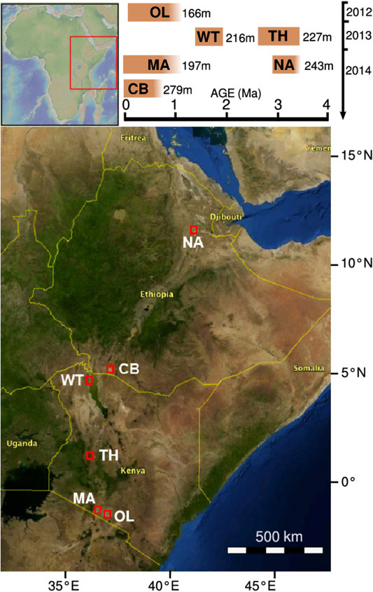
FIGURE 1. Drilling sites of the HSPDP. The graph on the top right indicates on its horizontal axis the estimated time spans before present that the drill cores correspond to. Its vertical axis indicates the year of core retrieval. From North to South: NA, Northern Awash; CB, Chew Bahir; WT, West Turkana; TH, Baringo Tugen Hills; MA, Lake Magadi; OL, Olorgesailie/Koora Plain. Map based on https://hspdp.asu.edu/?q=drill-sites and Cohen et al. (2016).

The investigation of sedaDNA is a relatively new approach in the study of deep sediment drill cores. Traditionally, the analysis of organisms in a sediment record often either relied on microscopy (then restricted to taxa with remnant hard structures, e.g. diatoms) or biogeochemical indicators for certain bio-productivities, an approach with very coarse taxonomic resolution (e.g. Stoof-Leichsenring et al., 2011). sedaDNA analysis does not depend on conservation of biomaterial that is suitable for microscopy and may hence considerably widen the range of taxa retrieved (e.g., limnoplanctic rotifers as good indicators of changes in salinity through time, Epp et al., 2010).

It is widely recognized that cold temperatures are beneficial for the preservation of aDNA in sediments or fossils (Pääbo et al., 2004; Epp et al., 2012; Hofreiter et al., 2015). In tropical settings, very high temperatures challenge sedaDNA preservation. Furthermore, during dry episodes, desiccation and subsequent exposition of the surface and littoral sediments to ultraviolet light and atmospheric oxygen likely reduce the chances of conservation of organic material, including DNA. Thus, most sedaDNA studies on sediment cores have focused on arctic or colder temperate regions (Parducci et al., 2017). For the few tropical sites included in sedaDNA studies (Epp et al., 2010; Epp et al., 2011; Stoof-Leichsenring et al., 2012), relatively recent sediments from short cores were analyzed. To date, only few publications cover high throughput sequencing (HTS) methods on sedaDNA of a tropical origin (Bremond et al., 2017). Although the first protocols for sedaDNA extraction were already published in the early 1980s (Torsvik, 1980), HTS has facilitated the implementation of paleogenetic approaches mostly for two reasons: first, it does not depend on any prior knowledge about the sedaDNA since it is independent of primers. Second, also smaller fragments that may not be amplified by classical PCR-based approaches can still be retrieved and sequenced (Dabney et al., 2013).

Studies on sedaDNA without any prior PCR amplification are usually compromised by a large part of the revealed metagenome originating from modern DNA of the prokaryote-rich deep biosphere (Magnabosco et al., 2019), which is barely informative about a site’s past ecosystem. As the extant deep biosphere mostly consists of prokaryotes, the eukaryotic fraction of a metagenome is particularly attractive for paleoenvironmental studies (Kisand et al., 2018). Not only are these DNA fragments much less likely to originate from extant organisms, but they also represent a large variety of typically studied groups, such as diatoms (Stoof-Leichsenring et al., 2012), rotifers (Epp et al., 2010), ostracods (Viehberg et al., 2018), or higher plants (Bremond et al., 2017).

DNA hybridization capture (a.k.a. target enrichment) has already been successfully applied to enrich low-concentration DNA-fragments of interest from aDNA samples including sediments (Slon et al., 2017; Murchie et al., 2020; Vernot et al., 2021). It relies on the ability of the DNA to hybridize with complementary nucleic acids, the so-called baits. These baits can either consist of DNA or RNA. While hybridized DNA fragments are retained using biotin-streptavidin binding, unwanted other fragments can be removed, at least in part, during washing steps following the hybridization. A major advantage is that the two hybridizing nucleic acid strands do not have to display perfect complementarity (Peñalba et al., 2014; Paijmans et al., 2016). Base mismatches and only partial overlap can be tolerated, such that also short DNA fragments, to which PCR primer annealing might have failed, can get enriched. This point is of particular importance since aDNA can have mismatches to sequences from extant organisms for various reasons, such as originating from a related species or sequence damage due to degradation. In addition, hybridization capture is less sensitive to contamination because DNA fragments of all lengths are targeted more equally, whereas PCR prefers longer fragments (Hofreiter et al., 2015).

Here we present a sedaDNA study on selected samples of the upper 70 m of two ∼280 m long lacustrine sediment cores from the paleolake Chew Bahir in Ethiopia (Foerster et al., in rev.). The objective of this metagenomic study is to contribute to the characterization of the past environment around the Chew Bahir basin and to test the feasibility of analyzing extremely degraded sedaDNA. We chose to utilize DNA hybridization capture for these sedaDNA studies, as hybridization capture has been proven superior to direct PCR amplification for highly degraded DNA (Dabney et al., 2013). We aimed at enriching a large spectrum of eukaryotic sedaDNA. A selection of metabarcoding marker gene sequences (from the established barcoding genes cox1 and rbcL for animals and plants, respectively) served as a template for hybridization capture bait design. Enriching for these two genes in defined taxa facilitates finding matches in reference DNA databases. In particular, cox1 is widely used as universal marker for species identification and constitutes the most sequenced genetic region of animal genomes (Pentinsaari et al., 2016) with over 8 million entries in the BOLDSYSTEMS database (July 2021) (Hebert and Ratnasingham, 2007). The use of rbcL is more limited, mainly due to small reference databases. BOLDSYSTEMS has not published the exact number of rbcL entries, but describes them as “very few” (https://www.boldsystems.org/index.php/IDS_OpenIdEngine, July 2021).

Regional Setting

Today, Chew Bahir is a saline mudflat at the southern border of Ethiopia at approximately 4.7071°N, 36.8524°E and an altitude of approximately 570 m asl (Foerster et al., 2012; Viehberg et al., 2018). While the tectonic basin is known to have been repeatedly filled with an up to 50 m deep freshwater lake during humid climate phases in the past, it is today under arid conditions and only episodically filled with a shallow water body during the rainy season (Foerster et al., 2012; Fischer et al., 2020a). The region around the Chew Bahir basin as the southern end point of the Main Ethiopian Rift (MER) is considered to be part of a prehistoric human migration corridor and the adjacent southwestern Ethiopian Highlands have been hypothesized to be a refuge area during episodes of drier climate (Brandt et al., 2012; Foerster et al., 2015). It is characterized by tropical climate with almost constant mean annual temperatures between 25 and 30°C and strong seasonality in precipitation with one rainy season named “Belg” from March to May and another named “Kiremet” from June to September (Foerster et al., 2012). The basin is filled with ∼3 km fluvio-lacustrine sediments, which record the climate particularly well, due to the sensitivity of the catchment area with large differences in relief to even minor shifts in the hydroclimate (Trauth et al., 2010; Fischer et al., 2020b). Deposits with coarser silt and sand beds are more abundant in the upper 100 m of the sediment column, while discrete layers of shell, fish bone, and plant debris could be identified throughout the entire core (Campisano et al., 2017).

Before the deep drilling campaign in the Chew Bahir basin started as part of the HSPDP in 2014, six short cores, up to 22 m long, had been collected in 2009–2010 from this site in pilot studies (e.g. Foerster et al., 2012; Trauth et al., 2018). Another 40 m long core from the center of the basin was drilled in March 2014 (Cohen et al., 2016; Viehberg et al., 2018). The pilot cores have been characterized in terms of material, age, and fossil record (Foerster et al., 2012; Foerster et al., 2014; Foerster et al., 2015; Trauth et al., 2015; Foerster et al., 2018; Trauth et al., 2018; Trauth et al., 2019). The fossils encompass fish bones, ostracods, molluscs, and diatoms (Foerster et al., 2012; Viehberg et al., 2018). Also, fossilized micro-charcoal was found as remains of plant material, but there is no pollen record, which is interpreted as a sign that biomaterial in the sediments is fairly degraded (Foerster et al., 2012), primarily due to the regular exposure of sedimentary deposits to oxygen. Among the molluscs, mainly shells of Melanoides tuberculata were found, a gastropod that is seen as an indicator for water levels below ∼10 m (Foerster et al., 2012). The diatom findings originate predominantly from Aulacoseira and Cyclostephanus, but the genera Nitzschia, Synedra, Cymbella, Cyclotella, and Achnanthes could also be identified. In contrast to the other species that prefer fresh water, Aulacoseira is tolerant to a broader range of salinity and pH and dominates especially in sections that correspond to presumably shallow water levels. In times of very low water levels, and therefore very saline and alkaline conditions, the diatom record declines sharply (Foerster et al., 2012; Foerster et al., 2014). Furthermore, as a typical plant remain, phytoliths have been examined in the third pilot core CB-03 in a section that corresponds to ∼5–12 ka BP (Trauth et al., 2018; Fischer et al., 2020a). The majority of phytoliths belongs to the group of mesic C4 grass types, but xeric C4 and C3 grass types are also found (Fischer et al., 2020b). Four ostracod species have been identified in the sediment core from the middle of the basin (HSPDP-CHB14-1A) (Viehberg et al., 2018): Limnocythere cf. borisi, Darwinula stevensoni, Ilyocypris sp., and Heterocypris giesbrechti. Limnocythere cf. borisi is known to have fragile valves and their good preservation is interpreted as evidence for undisturbed sedimentation.

These findings on bioindicators served as an orientation for the application of molecular genetic methods on the sediments from the Chew Bahir basin and were considered during bait design.

Materials and Methods

Core Drilling and Sampling

The sediment samples originate from two drill cores taken from the southwestern Chew Bahir basin in November-December 2014 (Figure 1). The duplicate cores were retrieved in close proximity to each other, core HSPDP-CHB12-2A at 4.7612°N, 36.7668°E and core HSPDP-CHB14-2B at 4.7613°N, 36.7670°E (Cohen et al., 2016; Campisano et al., 2017). They are 278.58 mbs (= meters below surface) (core HSPDP-CHB14-2A) and 266.38 mbs (core HSPDP-CHB14-2B) long and were merged into a composite core, ∼292.76 mcd (= meters composite depth, hereinafter written as ∼292.76 m for simplicity) long, after correlating the physical properties and imagery of the cores 2A and 2B (Arnold et al., 2021; Duesing et al., 2021; Roberts et al., 2021; Schaebitz et al., 2021; Trauth et al., 2021). Together they replenish missing data in each other and the composite core with ∼90% continuity will be referred to as one core in the following. According to the results of radiometric age determination and age modeling, this record represents the last ∼620 ka before present (Roberts et al., 2021).

The collected material consists of almost three metric tonnes of mostly calcareous clays and silts (Cohen et al., 2016). During transport and subsequent storing until further treatment, samples were kept at 4–10°C. The cores were sampled and are stored in the facilities of the National Lacustrine Core Facility (LacCore) of the University of Minnesota in Minneapolis, United States. Approximately 3–5 g of sediment per sample were transferred into 5 ml plastic falcon tubes without any buffer and kept at –80°C. Samples for sedaDNA analysis were taken at a resolution of 2 cm. During sampling, methods to avoid cross-sample and modern human DNA contamination were applied, in particular changing gloves between samples and removal of outer layers of the sediments. Since it was not known to what depth DNA was conserved in sufficient quality, 11 samples from the upper section of both cores down to 10 m were selected. When choosing samples, those with known occurrences of organisms (e.g., shell, plant, or bone remains) were preferred. One sample at the depth of ∼70 m was added to this study to explore whether deeper samples still deliver meaningful genetic data, resulting in a total of 12 samples. Another sample at 41.72 m was originally included, but discarded after sequencing, since it exhibited substantial amounts of contamination with putative modern human DNA. Throughout this article, we label our samples relative to their depths in the composite core. “A” or “B” in the sample IDs display whether the sediment sample originates from core HSPDP-CHB14-2A or HSPDP-CHB14-2B. The following sample number indicates the sample’s position in meters below surface of the respective core (mbs). Most samples are younger than ∼30 ka, with a single sample from ∼150 ka, according to the RRMay2019 age model of Roberts et al. (2021).

DNA Extraction and Library Preparation

All materials and chemicals that can persist UV sterilization were UV-treated before use. Tools and surfaces were treated with a DNA-degrading agent (DNA-ExitusPlusTM, AppliChem). All steps that involved unamplified aDNA were performed in dedicated aDNA laboratories. For every third sample a mock extraction (“extraction blank”) without any sample material was added. Gloves were changed between the opening of the tube of every sample. The samples were initially sampled at 3–4 g in order to work with the DNeasy PowerMax Soil Kit (QIAGEN), which is designed for input masses of up to 10 g. However, we moved to other protocols more suitable for highly degraded fragments. We decided against further subsampling the samples in order to avoid any (cross-) contamination. DNA extraction combined protocols published by Dabney et al. (2013) and Wales et al. (2014) with modifications for sediment samples by Pedersen et al. (2016). The amounts of lysis buffer were adapted to the sample size, resulting in 5 ml of lysis buffer (68 mM N-lauroylsarcosine sodium salt, 50 mM Tris-HCl pH 8.0, 150 mM NaCl, and 20 mM EDTA pH 8.0, with 1.0 ml 2-mercaptoethanol and 1.5 ml 1 M DTT added to every 30 ml immediately before extraction) being added to 3–4 g wet weight of sediment sample (all samples, except those at 2.17, 41.72, 71.65 m). After the overnight incubation at 37°C, the samples were centrifuged at 5,000 × g for 5 min. The approximately 2 ml of supernatants were further processed according to Dabney et al. (2013) using 650 µl PE buffer during the washing step. Samples at 2.17, 41.72 m (later discarded due to putative contamination), and 71.65 m were extracted in a later batch using 3 ml of the extraction buffer of the protocol of Dabney et al. (2013) to test applicability of this protocol to sediment samples. Samples at 0.93 and 5.21 m had a turbid, brownish eluate, and the samples at 2.17 and 71.65 m a turbid, light brownish one. The color originated from particles that could be removed by short centrifugation at low speed.

We used 20 µl of every extract, including the extraction blanks, for library preparation right after extraction based on a protocol by Gansauge and Meyer (2013), with modifications suggested by Korlević et al. (2015). As for extraction, for every third sample a mock library preparation (“library blank”) was performed. In this method, the Illumina P5 adapter is truncated at the 3’ end by five base pairs (GATCT) in comparison to the standard P5 adapter. Library preparation was performed with the following modifications: the optional step of removing deoxyuracils using the Afu (Archaeoglobus fulgidus) uracil-DNA glycosylase (UDG) was included. For cost reduction, the amount of Circligase II was reduced from 4 to 2 µl (100 U/μl) and as compensation, the incubation prolongated from 1 h to overnight in order to compensate for the smaller amount of enzyme. To account for this reduction, 2 µl more of nuclease free water were added to the uracil excision reaction in step 1 of the library preparation protocol. Two microlitres (10 U/μl) of the Klenow fragment of DNA Polymerase I were used, which allows for circumvention of the blunt-end repair in step 16 of the original protocol. According to this, the mastermix contained 0.4 µl of dNTP mix and additional 1.1 µl of nuclease free water. Incubation temperatures and times were adjusted to the different enzyme. The libraries were first incubated at 25°C in a preheated thermocycler for 5 min and then at 35°C for another 25 min. After library preparation, a qPCR was performed on 1 µl of sample, with three replicates per library, in order to estimate the optimal number of PCR cycles for indexing of the library molecules and library amplification (Basler et al., 2017). The underlying principle is that libraries with low DNA concentrations, in particular blanks, will need more qPCR cycles to reach the flexing point in the logistic growth curve. As compensation, these libraries will undergo more PCR cycles during library amplification than regular samples with presumably higher DNA concentrations. The qPCR was performed in a PikoReal 96 Real-Time PCR machine (Thermo Fisher Scientific TCR0096).

The reagents for library amplification and indexing comprised 44.8 µl of nuclease free water, 8 µl of 10 × AccuPrimeTM Pfx reaction mix (ThermoFisher Scientific), 0.8 µl of 2.5 U/µl AccuPrimeTM Pfx polymerase, 3.2 µl of P5 indexing primer, 3.2 µl of P7 indexing primer and 20 µl of each library. The PCR reactions were executed starting with 2 min at 95°C, followed by the number of cycles calculated according to Basler et al. (2017) consisting of 15 s at 95°C denaturation, 30 s annealing at 60°C and 1 min extension at 68°C. The libraries were cleaned up with the MinElute PCR Purification Kit (QIAGEN) following the manufacturer’s instructions. They were then quantified with the Qubit® 2.0 fluorometer and the distribution of DNA fragment lengths was measured with an Agilent 2200 TapeStation with a D1000 cassette.

DNA Hybridization Capture

Taxon-specific RNA-baits for hybridization capture were synthesized according to sequence templates. For animals, sequences of the mitochondrial cytochrome oxidase subunit 1 (cox1 or COI) gene were used as barcoding marker for species identification. The sequence of the chloroplast ribulose bisphosphate carboxylase large chain (rbcL) served as the universal barcoding marker for higher plants and diatoms (Wales et al., 2014). A set of selected target species was compiled based on a literature research and microscopic evidence. Results from the pilot core studies on paleolake Chew Bahir provided initial information on which potential target species to expect in the long core, including gastropod, teleost, and plant species (Foerster et al., 2012; Foerster et al., 2014). The “Atlas of the potential vegetation of Ethiopia” (Friis et al., 2011) provided an impression of the current flora around the Chew Bahir basin which was considered to select target plant species.

For all chosen taxa or their closest relatives, sequence information for the barcoding genes was retrieved from the GenBank sequence database (ncbi) between May and August 2017. Often, the sequences available at GenBank covered the gene loci only partially. In total, 223 metabarcoding sequences from 199 different species were collected (Supplementary Table S1). For these sequences, baits were produced by Arbor Biosciences^TM in form of a myBaits® Custom Target Capture Kit. The final set contained 19,584 baits, each at a length of 60 bp. The synthesized baits were short overlapping fragments representing the whole bait-template sequences of cox1 or rbcL of the respective taxon. The “tiling density” of the bait set was 4 ×, i.e., any base in a sequence was covered by four different 60 bp-baits. According to empirical experiences of the suppliers, one extra copy of baits with <28% GC content, one extra copy of baits with ≥50% and <60% GC content, and four extra copies of baits with >60% GC content were included in order to prevent capture biases. Ambiguous bases (e.g. the IUPAC code “Y” for pyrimidines) in the reference sequences were replaced at equal ratios with a single candidate base. Undetermined bases, indicated by an “N” in the DNA sequence, were always replaced with thymine, which is the standard procedure of the bait manufacturer. For taxonomic groups underrepresented in our taxon selection (e.g. there were far fewer bird than diatom species selected), two to three extra copies of each bait were added.

Hybridization capture reactions were performed using the myBaits® In-Solution Sequence Capture for Targeted High-Throughput Sequencing Custom Kit (designs with 1–20 k probes) by Arbor Biosciences^TM. The recommended input is 100–500 ng of library DNA, which equaled 7 µl of our libraries (DNA concentrations of amplified libraries between 14 and 72 ng/µl, extraction blanks 10–23 ng/µl, library blanks 9–15 ng/µl). In order to reduce the number of samples undergoing hybridization capture, the five extraction blanks (four from extraction batch one, one from batch two) and five library blanks were pooled separately, resulting in one pooled extraction blank and one pooled library blank. The capture experiments were conducted according to the manufacturer’s instructions with the following modifications: all capture reactions were incubated for 45 h at 55°C as recommended by the manufacturer for highly degraded samples. Due to the truncation of the P5-adapter in the library (according to Gansauge and Meyer, 2013), the kit’s standard blocking oligos were not used. Instead of adding 0.5 µl of the BLOCK#3 solution, 0.9 µl of 67 µM custom blocking oligos, which are suitable for the single stranded library, were added to each reaction.

Previous experiences show that dilution of commercial baits is a cost-effective way of hybridization capture, even of degraded DNA, without decreasing the yield substantially (Hawkins et al., 2016). Therefore, the RNA-bait solution was diluted 5 ×. The blocking solutions BLOCK#1 and BLOCK#2 were diluted 2 ×. All blanks of extraction and library preparation were pooled at equal volumes and included in the capture experiments as samples. In addition, a capture blank was added to the samples. The “Hybrid Bind & Wash” step was performed using a 96-well magnetic particle collector and Dynabeads® MyOne Streptavidin C1 beads. The captured DNA was eluted in 30 µl 10 mM Tris-HCl, 0.05% TWEEN®-20 solution at pH 8.0–8.5. Before library amplification, a qPCR was performed in order to determine a suitable amount of amplification cycles for each sample (Basler et al., 2017). The qPCR was performed in the same manner as for library preparation, except for using the primer pair IS5 (AATGATACGGCGACCACCGACAA) and IS6 (CAAGCAGAAGACGGCATACGAACA) (Meyer and Kircher, 2010). Subsequently, the captured libraries were amplified using Herculase Fusion II polymerase (Dabney et al., 2013) using the appropriate cycle number determined by qPCR (Basler et al., 2017) and the primer pair IS5/IS6 and cleaned with the MinElute PCR Purification Kit (QIAGEN), resulting in 20 µl for each library. DNA concentrations and fragment length distributions were characterized by Qubit® 2.0 fluorometer and by Agilent 2200 TapeStation (D1000 cassette) measurements.

Before hybridization capture, the libraries of all samples, except for the samples at 2.17 and 71.65 m, underwent direct shotgun sequencing on an Illumina Nextseq 500 platform, producing approx. 260,000 maximally 76 bp long single-end reads per sample. This will be referred to as ”shotgun data.” All twelve libraries that underwent hybridization capture were sequenced on an Illumina Nextseq 500 platform, producing approximately three million 76 bp single-end reads per sample. This will be referred to as “first round capture data.” A second round of hybridization capture was performed on the samples at 2.17, 2.48, 2.93, and 71.65 m. The second round of capture used the captured and amplified libraries of the first capture experiment as input for a second capture procedure, i.e., all steps of the hybridization capture were performed a second time. Sequencing conditions were the same as for first round capture data. The data resulting from this are referred to as “second round capture data.” The blanks were sequenced together with the respective sample libraries at the same depths as the samples, prior to capture (shotgun data) and after two rounds of hybridization capture.

Bioinformatic Analysis

All reads underwent adapter- and quality-trimming using cutadapt-2.6 (Martin, 2011) with the parameters -q 25 as quality cutoff, -m 30 as minimal sequence length, -O 1 as minimal overlap between sequence and adapter to be cut, and -n 3 to ensure removal of multiple adapter fusions. Duplicate reads were removed using the fastx_collapser of the fastx-toolkit-0.0.14 (Gordon and Hannon, 2010). The quality of the libraries was inspected using fastQC (https://www.bioinformatics.babraham.ac.uk/projects/fastqc/). The sequences were assigned to taxonomic groups using Kraken-2.0.7 (Wood and Salzberg, 2014). A Kraken2-k-mer database of all sequences of GenBank’s nt database (version 2019-01-03) with a maximum size of 100 GB was built prior to applying the Kraken2 tool to the datasets. The commonly used aDNA verification tool mapDamage (Ginolhac et al., 2011) relies on identification of mainly C-to-T substitutions at the 5’- and 3’-termini of the sequences that are typical for aDNA in single stranded libraries. However, identifying such base substitutions requires a reference, which was not available for all taxa potentially contained in the samples’ complex metagenomes. Furthermore, aDNA damage patterns, while indicative of aDNA authenticity, may compromise correct taxonomic assignment of reads. For this reason, the libraries underwent UDG-treatment (Gansauge and Meyer, 2013) (see DNA Extraction and Library Preparation) in order to remove uracils and reduce damage patterns and thus increase chances of correct database matches in the Kraken2 analysis, at the expense of being unable to further investigate aDNA-specific damage patterns. Visualization and inspection of the results was realized using the online tool Pavian metagenomics data explorer (Breitwieser and Salzberg, 2020). All statistical analyses (including PCA) were performed in R version 3.6.3, using the packages ggplot2, ggforce, reshape2, dplyr, graphics, RColorBrewer, wesanderson, and seqinr. Using custom R scripts, all species that displayed relevant online BLAST hits to the Illumina P7 adapter were excluded from the analysis and removed from the counts of reads at all taxonomic levels. This applied to all species of the following genera: Cyprinus (Teleostei), Camelus (Mammalia), Wasmannia (Hexapoda), Lasthenia (Asteraceae), Gossypium (Malvaceae), Fargesia (Poaceae), Eimeria (Alveolata), Plasmodium (Haemosporida), and the Staphylococcus phage Andhra. This step was implemented in all analyses underlying the figures in this publication. After performing Kraken2 analysis, assignments to the genus Homo were abundant across most samples (Supplementary Tables S11–S16). However, because of possible contamination or other possible artifacts, i.e. biases to human sequences in the reference database, these assignments were not considered and hence excluded from further analysis. The counts of these omitted genera are, however, available in the tables created with Pavian (Supplementary Tables S11–S16). Sequence length distributions were assessed before and after Kraken2 analysis, using the R package seqinr. In order to obtain read distributions of distinct taxa, all reads assigned to these taxa were filtered from the duplicate removed fasta files using the script extract_kraken_reads.py with the --include-children option from KrakenTools (https://github.com/jenniferlu717/KrakenTools, July 2021).

Enrichment success was evaluated with regard to the marker sequences from which the 60 bp-baits were designed. In all datasets, the fraction of reads that show significant sequence similarity to cox1 and rbcL was estimated using Hidden Markov Models (HMMs). The HMM was produced with the nHMMER function of the HMMER 3.1b1 tool collection (Wheeler and Eddy, 2013). Each HMM required a seed alignment in order to train the model. For each marker gene, the seed alignment was constructed of representative DNA sequences from a broad range of species across the tree of life using MAFFT v7 with the nwildcard option in order to align undetermined nucleotides (Katoh et al., 2002). The accession numbers of these sequences are noted in the Supplementary Tables S2, S3.

The precision of taxonomic assignment depends on the degree of sequence conservation of the reference. The Shannon entropy served as an approximation of the degree of conservation across eukaryotes in the different domains of the cox1 gene. Applied to DNA sequence alignments, the Shannon entropy describes the diversity of each nucleotide position (i.e. column) of an alignment. Estimation of the Shannon entropy of a cox1 multiple sequence alignment was carried out with Python 2.7 (https://gist.github.com/jrjhealey/130d4efc6260dd76821edc8a41d45b6a 2020-10-26), applying a moving average of ten. In order to avoid distortion due to different nucleotide coverage at the positions of the MSA, only full length cox1 sequences were aligned with default settings in MAFFT v7. The accession numbers of these selected sequences are listed in the Supplementary Table S4. For better visualization, entropy scores were inverted by subtraction from the maximal possible value, which was ∼2.33 when assuming five possible nucleotide states (ATCGN). This way, a high value on the vertical axis equals a high estimated degree of conservation (i.e., a low entropy).

While Kraken2 served as a comprehensive approach to unravel the sample’s taxonomic profiles, enrichment patterns and efficiency of our bait set composition was evaluated with bwa. Specifically, all quality-filtered reads were mapped back to a collection of cox1 and rbcL sequences using bwa v0.7.17’s mem-algorithm (testruns with bwa aln with seeding disabled are shown in Supplementary Table S18). This collection of cox1 and rbcL sequences consisted of all sequences used for bait design, as well as 14 marker sequences of further potentially interesting species: Vertebrata thuyoides (Rhodophyta), Gracilaria salicornia (Rhodophyta), Leishmania tarentolae (Euglenozoa), Trypanosoma cruzi (Euglenozoa), Tapes belcheri (Bivalvia), Picocystis salinarum (Chlorophyta), Micromonas pusilla (Chlorophyta), Alcelaphus buselaphus (hartebeest antelope, Mammalia), Haphsa durga (Hexapoda), Homo sapiens (Mammalia). These additional species were identified post hoc by inspecting the Kraken2 results for taxa with relatively high read numbers and potential biological relation to the environment of Chew Bahir in eastern Africa. Species with chloroplasts were represented with both cox1 and rbcL sequences. Samtools 0.1.19 idxstats was used to count reads per cox1 or rbcL sequence. Samtools view in combination with shell commands served for filtering and counting reads according to their mapping quality score (MAPQ) and multi-mapping properties. The distribution of mapped reads was inspected using igv 2.7.2. From all cox1 gene sequences, those regions to which five or more reads mapped were copied into a separate fasta file. The sequences of this file were added to the MSA of full length cox1 gene sequences using MAFFT v7 with the --addfragments and --keeplength options. This alignment was visualized in Jalview 2.11.1.0. All full-length sequences were removed, leaving only the fragments that indicate the regions to which five or more reads mapped. The panel that visualizes the coverage of each column of this alignment (“occupancy”) was exported as cox1 mapping hotspots and aligned with the inverse Shannon entropy estimates to test for a relationship between the reads’ likelihood to map to a particular region in the cox1 gene and that region’s degree of sequence conservation.

Results

Extraction Success and Library Quality

The DNA extracts of all samples displayed relatively low DNA concentrations in the QuBit measurements, all below 4 ng/µl, but often even below the detection limit of 0.5 ng/µl. The samples differed considerably in appearance after extraction, with most of the samples showing transparent, colorless DNA extracts, but the samples at 0.93, 2.17, 5.21, and 71.65 m having turbid, light to medium brownish particles that could be removed by short centrifugation at low speed. None of these samples containing sediment remnants showed notably different results in subsequent analyses. The two samples at 2.17 and 71.65 m, that were extracted following exactly the protocol of Dabney et al. (2013) also did not display any notably different results from the other samples that were extracted according to a combination of the protocols by Wales et al. (2014), Pedersen et al. (2016), and Dabney et al. (2013).

Read length distributions (Figure 2) show that for all samples except those at 0.93 and 6.36 m, after one round of capture, reads of 71–76 bp length are the most abundant with counts in the hundreds of thousands per each possible length. Shorter reads of 30–70 bp show counts in the tens of thousands. Read length distributions of taxonomic groups that were classified by Kraken2 (Figure 3) mainly follow the general read length pattern of their respective sample (cf. Figure 2). Reads classified as bacterial are more abundant than reads classified as eukaryotic at any given length. In contrast, after two rounds of hybridization capture, for samples at 2.17, 2.48, and 2.93 m, the reads assigned as eukaryotic occasionally outnumber the putative bacterial reads (Figures 4, 5). The read length distributions of the blanks for DNA extraction and library extraction generally resemble those of the samples, however, with in most cases lower read numbers and some deviations in the library extraction blanks (Supplementary Figures S1, S2; Figures 4, 5).

FIGURE 2

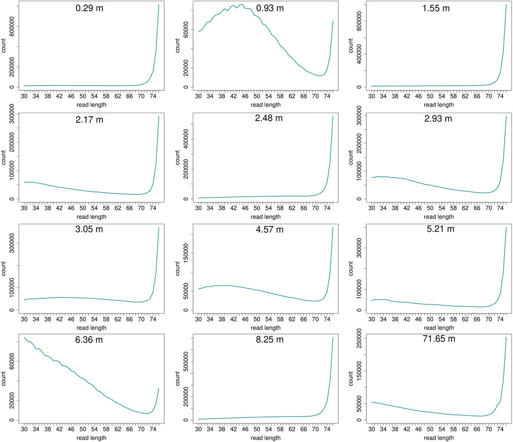
FIGURE 2. Read length distribution of all reads after duplicate removal for first round capture data. Samples at 0.93 m and at 6.36 m depth display a larger proportion of shorter reads in relation to the maximum possible length of 76 bp. However, this effect is less pronounced when taking into account the high fluctuation of absolute read numbers on the y-axis. The curve of samples that have much fewer short reads in relation to longer reads (>70 bp) may appear flat, but the counts usually still range in the tens of thousands (0.29 m: at 30 bp 13,023 reads counted, at 70 bp 23,980; 1.55 m: at 30 bp 11,802, at 70 bp 28,943; 2.48 m: at 30 bp 6,855, at 70 bp 25,867; 8.25 m: at 30 bp 7,997, at 70 bp 41,531).

FIGURE 3

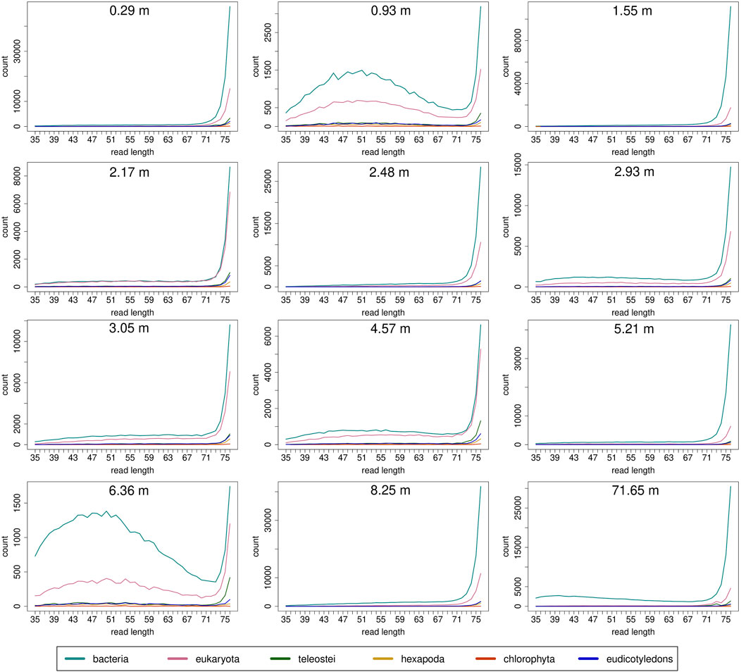
FIGURE 3. Read length distribution of reads assigned to selected taxonomic groups after Kraken2 analysis for first round capture data. Read groups were filtered by GenBank TaxIDs using KrakenTools (https://github.com/jenniferlu717/KrakenTools, July 2021). Read length distributions mainly follow the trends of the distribution before entering Kraken2 analysis after duplicate removal. Note that read counts can be substantially smaller as in Figure 2 because only reads that could be assigned are displayed.

FIGURE 4

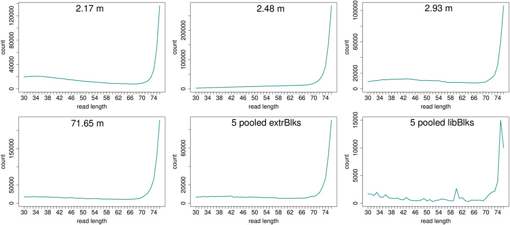
FIGURE 4. Read length distribution of all reads after duplicate removal for second round capture data. Longer reads (>70 bp) dominate all samples. The pooled blanks (one for mock extractions “5 pooled extrBlks” and one for mock library preparations “5 pooled libBlks”) display lower read numbers compared to samples, yet the difference is not always more than 2-fold (e.g. compare sample 2.93 m and five pooled extrBlks).

FIGURE 5

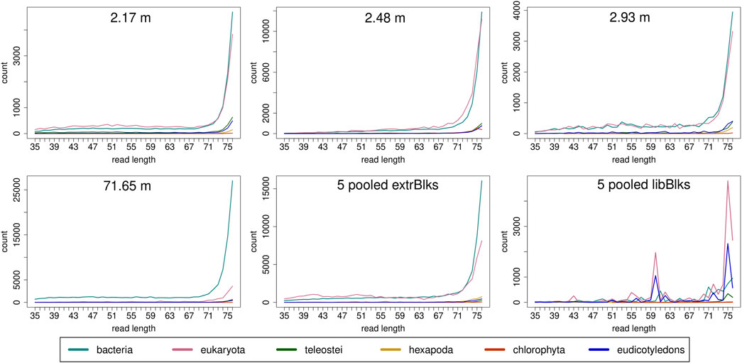
FIGURE 5. Read length distribution of reads assigned to selected taxonomic groups after Kraken2 analysis for second round capture data. In all samples, except for the sample at 71.65 m, for some read length classes, putative eukaryotic reads are found in higher numbers than putative bacterial reads. Note that the read length distribution for the pool of extraction blanks resembles those of the samples, especially of the oldest sample at 71.65 m, with a particular large bacterial fraction. The read length distribution in the pooled library blanks, however, deviates more from those of the samples and displays large frequency changes among adjacent length classes.

Enrichment Success

The main aim of the hybridization capture experiment was to enrich marker sequences from a broad range of eukaryotic species. After trimming and quality filtering, all reads were scanned for putative marker sequences (cox1 or rbcL). The fraction of reads that aligned to the HMM and therefore presumably originated from a marker gene was determined for every sample as parts per million (PPM) and ranged from 0 to 23 for shotgun, 67 to 2,461 after the first round of capture and 805 to 28,305 after the second round. In summary, after one round of capture the fraction of marker reads increased 15 to 413-fold (Figure 6). After a second round of hybridization capture, the fraction of marker reads compared to that after the first round increased 10 to 36-fold. For the samples at 2.48 and 2.93 m, from which sequence data of all three sequencing stages (shotgun, first round capture, second round capture) is available, this resulted in overall 580 and 1,769-fold increases, when comparing simple shotgun sequence data and second round capture sequence data (Figure 6).

FIGURE 6

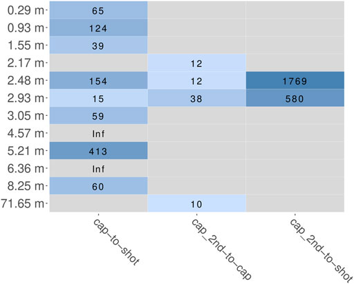
FIGURE 6. Fold change of relative abundance of marker reads (cox1 and rbcL summarized) estimated by HMMs. Coloration according to log10 value of fold change. Grey panels indicate inability to calculate fold change, either because of a zero delimiter (“Inf”) or missing data (because a sample was not included in the respective experiment). “cap”, first round capture data; “shot”, shotgun data; “cap_2nd”, second round capture data.

Taxonomic Classifications

Assignment of Reads after Sequencing

Among all raw datasets across all samples, between 87 and 98% (mean >96%) of all sequence reads did not yield a phylogenetic placement. On average, for each of the three sequencing stages, between 11 and 26% of the reads were discarded because they were either too short, consisted of adapters only, or did not meet the minimum quality score. Another 1% (average for shotgun samples) to 50% (average for samples after second round of capture) were discarded because they were inferred to constitute PCR duplicates. The more capture reactions and subsequent library amplifications were applied, the more PCR duplicates were removed (Figures 7A–C). After trimming and duplicate removal, an average of 93–95% of all reads that entered the Kraken2 analysis remained taxonomically unassigned.

FIGURE 7

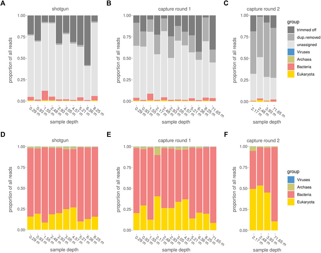
FIGURE 7. Categorization of reads. (A–C) Assignment of raw reads, including the fractions of reads that did not pass quality or size filtering (“trimmed off”), PCR duplicates (“dup.removed”), and failed taxonomic assignment (“unassigned”). (D–F) Taxonomic assignment of reads which passed the quality control steps and were retained for further analysis. (A,D): shotgun data, (B,E) first round capture data, (C,F) second round capture data (only applied to a subset of samples).

Proportions Between Domains of Life

After one round of capture, the ratios between the different organismal domains change. Specifically, the percentage of reads determined as eukaryotic increased, while the percentage of reads considered bacterial decreased (Figures 7D, E, 8A). A second round of capture further increased the number of reads assigned to eukaryotes, albeit to a different extent across taxa (Figures 7F, 8B).

FIGURE 8

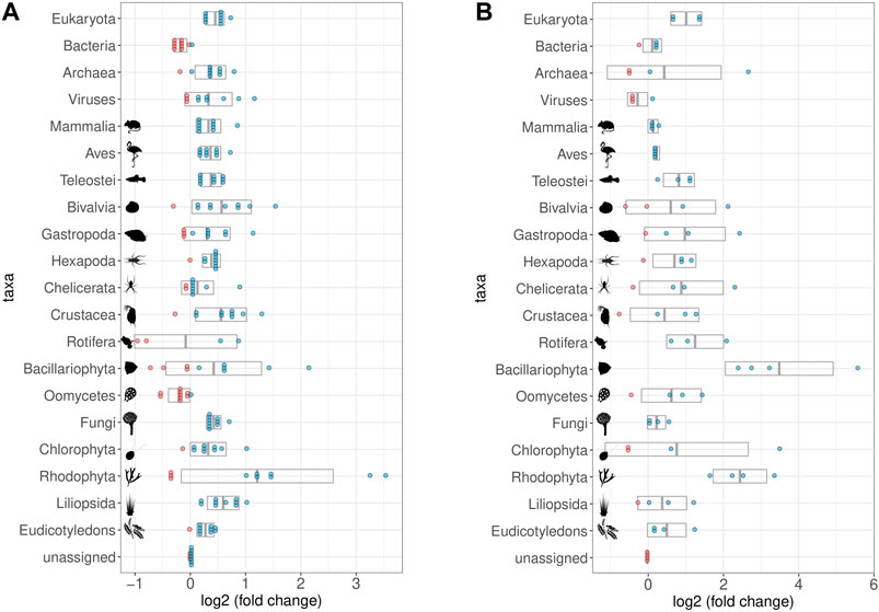
FIGURE 8. Impact of Hybridization capture on different taxa and samples. log2 of fold changes of relative abundances of reads assigned to selected taxa. Dots represent the single samples with increased (blue) or decreased (red) abundance of the respective taxon; grey boxes display the mean value (middle) ± standard deviation. All taxa contained in the bait set are displayed, as well as some that were relatively abundant despite not being part of the bait set (Viruses, Chelicerata, Oomycetes, Fungi, Chlorophyta, and Rhodophyta). Note that fold-change calculations are less precise for taxa with few reads assigned to them (cf. Figure 9 for taxon-specific read counts). (A) Relative abundances in the first round capture data compared to those of the shotgun data. The relative abundance of eukaryotic reads increased at the expense of bacterial reads. (B) Relative abundances in the second round capture data compared to those of the first round capture data. The decrease of the bacterial fraction could only be observed after the first round of hybridization capture. Pictograms from phylopic.org courtesy of Sergio A. Muñoz-Gómez, Harold N Eyster, Julie Blommaert based on photo by Sofdrakou, Melissa Broussard, and Soledad Miranda-Rottmann. License: https://creativecommons.org/licenses/by/3.0/.

Number of Reads Assigned to Specific Taxa

In the results of the Kraken2 analysis, the bacterial genus Pseudomonas is the most frequent genus in all datasets, including all blanks (Supplementary Tables S11–S16). Among the retained reads assigned to eukaryotes, some taxa are more prominent than others, in particular mammals, birds (Aves), fish (Teleostei), insects (hexapods), and dicotyl plants, a pattern that is quite stable across all samples of different depths and across shotgun and capture data (Figures 9A, B, D; Table 1 depicts most abundant genera). A smaller fraction of the reads was assigned to Bivalvia, Gastropoda, Crustacea, Rotifera, and Bacillariophyta (diatoms). Notably, there was no systematic decrease or altered assignment pattern in the lowermost sample (71.65 m), as compared to the samples from the upper 10 m of the core.

FIGURE 9

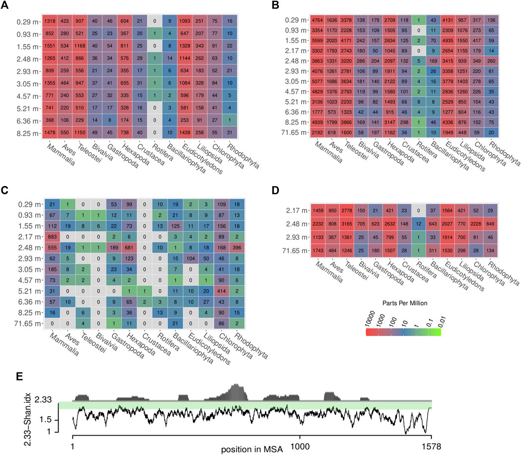
FIGURE 9. Relative and absolute abundances of reads assigned to different eukaryotic taxa across samples and methods. Colors represent parts per million (ppm) of reads, grey: no reads. The absolute number of reads is written in the center of the colored tiles. (A) shotgun data, (B) first round capture data, (C) first round capture data mapped to cox1 sequences of the respective taxa, (D) second round capture data, (E) propensity of reads to map to particular regions in the cox1 gene (distribution in upper part) and degree of sequence conservation (lower part), which is estimated by a moving average (n = 10) of its Shannon entropy per column. The entropy score was subtracted from the maximal possible value (2.33 allowing five nucleotide states: ATGCN) for better representation of estimated sequence conservation. This way, high values on the scale correspond to a high degree of sequence conservation which coincides with a high propensity of reads to map to these regions. Note that values for Mammalia did not include reads assigned to Homo sapiens, to avoid impact of possible contamination (see Materials and Methods for details).

TABLE 1

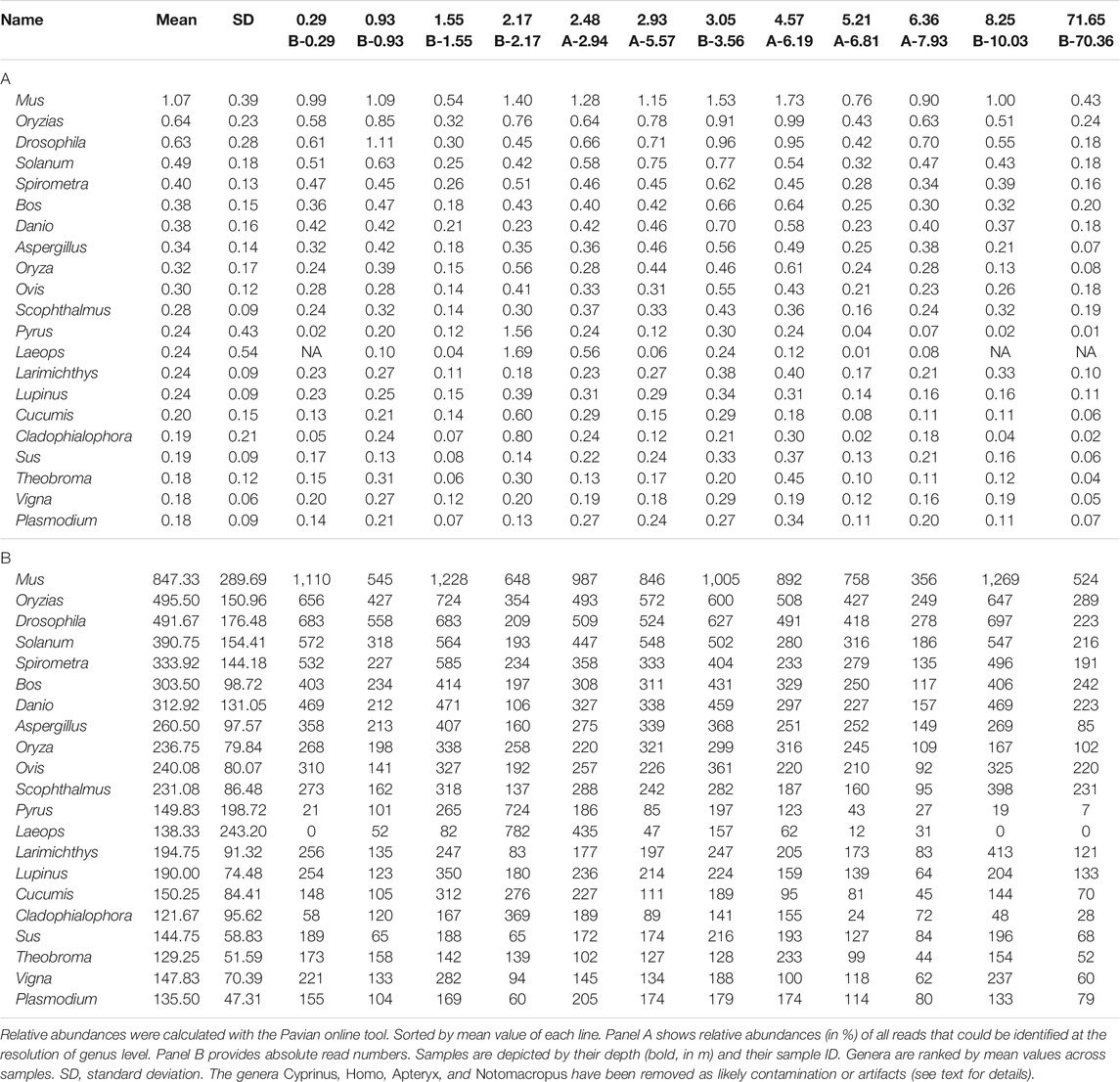
TABLE 1. Most abundant eukaryotic genera in the first round capture dataset.

Some taxonomic groups, such as red (Rhodophyta) and green algae (Chlorophyta), were rather prominent in the Kraken2 results (after one and two rounds of capture), albeit no taxon-specific sequences had been included in the bait set. This pattern remained, even if the data were restricted to sequences assigned to the barcoding gene cox1 used for hybridization capture (Figure 9C).

In both PCA and hierarchical clustering, the samples did not group according to their depth (Supplementary Figure S3). The sample at 2.48 m, which had the highest number of reads assigned to the barcoding gene cox1 (Figure 9C), stood out in the corresponding PCA plot (A-2.94 in Supplementary Figure S3).

The reads were further mapped back to the template sequences of the bait set and 14 additional cox1/rbcL sequences (see Material and Methods) using the bwa mem algorithm (Supplementary Table S17). When mapping the reads back to the cox1 sequences of the bait set, some previously detected taxa could not be observed at all (grey coloring in Figure 9C). Mammalia, Hexapoda, and Chlorophyta form the groups to which most reads could be mapped. In this analysis, the oldest sample at 71.65 m yielded a considerably smaller number of reads than the samples of the uppermost 10 m of the core. Overall, much fewer reads mapped back to the bait set template sequences than there were reads that could be classified in Kraken2. This resulted in a patchy representation of some taxa (Figure 9C) that loosely, but significantly correlated with the results obtained by Kraken2 (ρ = 0.239, p = 0.002). Across all species and samples, reads preferentially mapped to particular regions of the cox1 gene (Figure 9E). From a representative alignment, the Shannon entropy index was calculated (for a moving window of 10 nucleotide sites) as a proxy for sequence conservation at different positions of the cox1 gene. The number of reads mapped to regions of the cox1 gene and that region’s estimated conservation were significantly correlated (ρ = 0.414, p < 0.001). Regarding abundant eukaryotic taxa, there is a sharp contrast between the two assignment methods Kraken2 and bwa mem (Figure 10): reads assigned to Hexapoda (insects) were very abundant according to both analyses, but Kraken2 inferred teleost fish as the most abundant taxon. In contrast, only few reads were assigned to teleost fish in the bwa mem analysis. Here, besides insects, a large fraction of reads was assigned to green algae (Chlorophyta). Interestingly, in the bwa mem analysis, there were marked fluctuations among samples retrieved from different depth in the respective abundance of reads assigned to either insects or green algae (Figure 10).

FIGURE 10

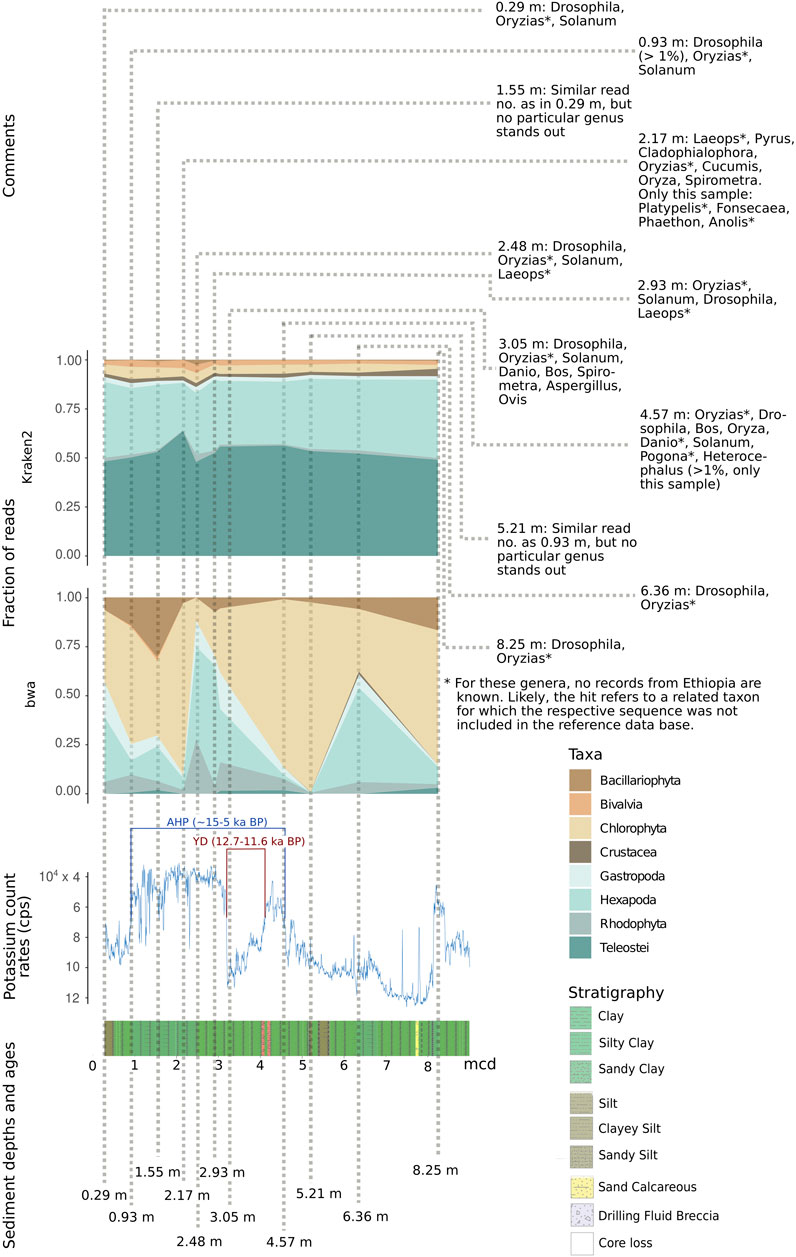
FIGURE 10. Relative fraction of reads assigned to selected abundant eukaryotic taxa with the two assignment tools Kraken2 and bwa mem, relative to depth (in m) as well as potassium count rates (inverted scale) and stratigraphy in the respective sediment layer. For each sample, the most abundant eukaryotic genera are depicted. AHD, African Humid Period; YD, Younger Dryas. Note that—due to incompleteness of reference databases—reads could be assigned to genera so far unreported for Ethiopia (marked *). They may refer to related taxa not included in the reference database. Potassium count rates in counts per second (cps, note that y-axis is inverted) (Trauth et al., 2021).

Discussion

Challenges of sedaDNA Metagenomics

Working with ancient sediment samples provides two main challenges: first, the deeper the sample from below the earth’s surface, the older and the more fragmented is the sedaDNA. Second, sediment samples regularly contain enzyme inhibitors. DNA extracts from sediment samples are known to contain DNA polymerase inhibitors, mainly humic acids (Wales et al., 2014; Parducci et al., 2018). Our DNA isolation protocols were tailored towards removing humic acids as much as possible, while retaining authentic sedaDNA. These two aspects, short fragment recovery and inhibitor removal, constitute a trade-off, since inhibitor removal requires additional processing steps, whereas small fragment retention rather implies keeping the number of processing steps at a minimum.

Generally, abundant eukaryotic taxa are detected throughout all samples and preparations, without any obvious systematic change relative to age/depth. The lowermost sample from 71.65 m (corresponding to ∼152 ka according to the directly dated RRMay2019 age model of Roberts et al., 2021) produced fewer reads, yet was inconspicuous with regard to taxon assignment (Figure 9). Notably, this reduction in read numbers by depth was most apparent in our gene-specific analysis, i.e. when considering only reads mapping to the cox1 barcoding gene (Figure 9C). This result meets the expectation that the amount of detectable authentic sedaDNA should decrease with age/depth. As a consequence for future DNA extractions from more samples, the samples could be processed in batches of similar depths in the core in order to minimize contamination of the samples with lower sedaDNA contents (presumably, the oldest ones) with DNA of more recent origin.

An important assumption for the paleogenetic analysis is that the DNA obtained is indeed ancient. This is rather difficult to test for in metagenomic sediment samples. Many of the sequences were assigned to microorganisms and likely originate from the deep biosphere, but are not necessarily ancient. Due to the complexity of metagenomes, the use of reference-based tools for aDNA content estimations, such as mapDamage (Ginolhac et al., 2011), is very limited. Therefore, other authenticity criteria for aDNA needed to be considered (e.g. Hofreiter et al., 2001; Walker, 2009). For this study, the criterion of using dedicated aDNA laboratories and including mock extractions and library preparations (“blanks”) was fulfilled for all laboratory processes. We assume that especially the extraction is a very critical step for potential cross-contamination. This assumption is based on the structural similarities between the sequences from sediment containing samples and those from the extraction blanks. Library blanks were produced one day after extraction, under the same precautions (i.e. changing gloves between opening sample tubes), yet differed from the extraction blanks and samples by lower read numbers and a more deviate read length distribution pattern (Supplementary Figures S1, S2; Supplementary Table 5). Pooling of blanks prior to hybridization capture is more economic and can avoid errors by reducing the number of samples to be handled in the laboratory. However, judging from our results, we argue that this option should be used with care because it reduces the ability to identify possible cross-contamination. To minimize cross-contamination, samples should be processed in as small batches as economically possible. This is particularly relevant in metagenomic studies, as cross-contamination across biological samples can hardly be detected and can be further inflated by amplification during library preparation and hybridization capture.

Our DNA extracts and libraries showed the typical low DNA concentrations and qPCR results experienced in other aDNA studies. The read length distributions (Supplementary Figures S1, S2; Supplementary Tables S2–S5) display short reads (30–70 bp), which indicates advanced DNA fragmentation, consistent with an ancient origin of the recovered sequences. Still, in most samples the majority of reads are longer (70–76 bp, 76 bp constitutes the maximal length possible). This fraction could originate from the deep biosphere, representing modern, mostly prokaryotic DNA, which is expected to be abundant in most samples. Samples with a less pronounced longer fraction, such as at 0.93 and 6.36 m, could indicate regions of less rich deep biosphere, presence of inhibiting agents, such as humic acids (Wales et al., 2014; Parducci et al., 2018), or unconscious methodological inconsistencies during lab processing. Ideally, the eukaryotic domain would be larger in the shorter read length range (30–70 bp). This would indicate a mainly eukaryotic origin of fragmented DNA. However, this was only partly observed after two rounds of hybridization capture (Figure 5). A possible reason is that fragmented ancient bacterial DNA is very likely also present. It must be emphasized that the assessment of read length distributions by taxonomic groups is always biased towards longer reads, as a read’s likelihood to be taxonomically classified increases with increasing read length. Tools for metagenomic aDNA authentication are currently under development. In the meantime, further analysis of samples from Chew Bahir may omit the UDG treatment (at least for some samples), such that reads could be mapped to a selection of species and be subsequently assessed for aDNA-typical damage patterns with mapDamage (Ginolhac et al., 2011).

Effects of Hybridization Capture on Ancient Metagenomes

In metagenomic analyses, many experimental and analytical decisions constitute explicit or implicit filters and hence influence the outcome. This is particularly true for the compilation of the bait set used for hybridization capture. The choice of target genes and species, the species’ evolutionary relationships and sequence divergence, as well as their numerical representation in the baits is likely to influence the taxon representation in the outcome. Within the scope of our study, the effects of the bait set species composition cannot be disentangled from other putative filters in the downstream analysis. Consequently, absolute abundances could not be inferred and cross-taxa comparisons of relative abundances should keep these potential biases in mind. Still, as the same filters were consistently applied across samples, we argue that—with all caution—shifts across strata of different depth in their relative abundances of reads assigned to specific taxa (Figures 9, 10) may reflect real shifts in the abundances of the respective taxon-specific sedaDNA.

We could demonstrate that hybridization capture led to an enrichment of both eukaryotic taxa (relative to prokaryotes) and of targeted barcoding sequences (cox1 and rbcL). The enrichment worked best for conserved regions of the target genes (Figure 9E). Consequently, taxa related to those for which the baits were designed could also be enriched. Sometimes even more distantly related taxa were enriched, such as Rhodophyta that had no close relatives in the bait set, yet they were enriched not only in the results of the Kraken2 analysis (Figure 8), but also in the first round capture datasets restricted to reads mapping back the target gene cox1 (Figure 9C, bwa-based analysis). As a consequence of this cross-taxa enrichment, baits complementary to any primate species should rather be excluded (unless they constitute the explicit focus of the study), as this could massively increase the enrichment for modern human contaminant DNA.

In the taxonomic assignments, Oomycota (water molds), Cladophialophora (Fungi), and Cryptococcus (Fungi) were often among the putative taxa which had left DNA traces in the sediment. It is not clear if the corresponding DNA fragments originate from ancient or extant populations. In case they originate from aDNA, they could be abundant and potentially ecologically informative of Chew Bahir’s past biosphere. Alternatively, these groups could be part of the deep biosphere, i.e. contributing modern DNA. A possible experimental procedure to investigate whether a taxon contributes modern DNA as part of the deep biosphere could be to target longer DNA sequences typical for modern DNA by PCR (Vuillemin et al., 2017).

Applying a second round of hybridization capture led for all samples to a further increase in the number of reads with taxonomic assignment and a decrease in putative contaminant/artifact reads (Homo or Cyprinus), but also yielded a higher fraction of PCR duplicate reads, which seems plausible as it involves another library amplification step. The Kraken2 results in the second round capture data featured two abundant aquatic eukaryotic genera, the flatfish Laeops and the green algae Micromonas that were not among the most abundant genera after only one round of hybridization capture. Assessing the validity of these assignments remains challenging, given the low reliability of current metagenomics software in taxonomic resolutions below family level (Sczyrba et al., 2017). Ultimately, the implementation of a second round of hybridization capture on metagenomes yields a slight overall increase in relative abundance of putative eukaryotic marker reads and identifies additional potentially interesting genera, at the expense of overall more amplification artifacts and a decreased absolute read number retained as presumably authentic.

The sensitivity of both our shotgun and hybrid capture approach appears superior to direct PCR on sedaDNA: in pilot studies (Krueger, Hofreiter, Tiedemann, unpublished), no PCR products could be produced on the sedaDNA not even from the uppermost sediments of Chew Bahir when using primers for diatoms or rotifers that were successfully applied to other eastern African sediment samples (Epp et al., 2010; Stoof-Leichsenring et al., 2012).

Reliability of Taxonomic Assignments

DNA sequence content in publicly available databases is taxonomically biased, with overrepresentation of so-called “model organisms” (e.g. Mus musculus, Drosophila spp., Bos taurus, Solanum spp.). In turn, taxa of current and past ecosystems of southern Ethiopia may be underrepresented. This may lead to an assignment bias towards model organisms (Kunin et al., 2008; Parducci et al., 2017). This bias becomes exacerbated in shotgun approaches, as retrieved sequences could originate from any gene of any taxon present in the sedaDNA. Abundant assignment to model organisms could indeed be observed in all our samples, even when applying stringent criteria.

Species identification based on established barcoding genes (cox1, rbcL) should be generally more reliable, as these genes have been sequenced in a much larger set of taxa. Yet, in the vast majority of recent publications, the performance of cox1 as metabarcoding marker is evaluated only for specific taxonomic groups. It is also important to consider that GenBank’s nt database is essentially an uncurated database, hence unconsciously propagating errors in the taxonomic and/or gene assignment of the submitting authors. For example, some sequences published as “COI” (cox1) in GenBank actually are nuclear copies of mtDNA that have become pseudogenes, so-called “numts” (Buhay, 2009). It has been argued that a considerable number of cox1 sequences derived from non-target taxa and result in wrong database entries (Mioduchowska et al., 2018). For some taxa and regions, the sequence databases are also incomplete even for the barcoding genes. Especially Rotifera and Ostracoda seem to be understudied or underrepresented in sequence databases (Curry et al., 2018), which could explain the very low number of assignments to these taxa in our study. Boessenkool et al. (2014) demonstrate with the example of a high-altitude lake in eastern Africa that a custom-made sequence database of the regional vegetation can facilitate species identification in subsequent metabarcoding analyses. These authors argue for an integrated analysis of a local database and large global databases, such as GenBank. The usage of rbcL as marker in metabarcoding faces similar challenges as cox1. The Consortium for the Barcode of Life plant working group recommends using rbcL together with the marker matK for sufficient discriminatory power (Janzen, 2009). However, the reference databases for rbcL are much smaller (e.g. https://www.boldsystems.org/index.php/IDS_OpenIdEngine, July 2021). Better database coverage of the earth’s plant biodiversity seems to be key for reliable taxonomic assignments. The Barcode Of Life Data System taxonomy identification engine only accepts cox1 or rbcL sequences of at least 80 bp length. Retrieving sequences of that length seems currently beyond feasibility in our study on the Chew Bahir drill core, except for perhaps the uppermost sediment layers.

The more precise the taxonomic classification of the sedaDNA fragments, the more precise can be the conclusions drawn from their presence. The extensive study of eastern African diatoms by Gasse et al. (1995) illustrates how even diatom species of the same genus can have quite divergent, non-overlapping tolerances for abiotic factors.

Benchmarking studies (Lindgreen et al., 2016; Sczyrba et al., 2017) point out that most metagenomic assignment tools, including Kraken2, do not perform very well at low taxonomic levels (species/genera), but can reliably assign to family level and above. These benchmarking studies focused on prokaryotes, while systematic assessments on the performance of current assignment tools for eukaryotic reads in a metabarcoding framework are still lacking.

Possible Inferences About Biodiversity in the Chew Bahir Basin in Response to Environmental Conditions

To limit biases in taxon assignment, we generally assigned our reads retrieved from the upper 70 m of the Chew Bahir drill cores to higher eukaryotic taxa (above family level). Here, inferred taxa generally resemble organisms known to occur in southern Ethiopia (Figures 8–10), with the exception of Rhodophyta, for which we could not find any African inland record in the literature. In the assignments produced by Kraken2, reads were searched against the entire GenBank nt database (Figures 8A,B,D, 9A,B,D). Differences were more prominent across taxa than across sampling depth/age, such that a putative correlation to environmental changes throughout the studied time period is not directly apparent. If we, however, focus only on the reads assigned to our barcoding marker gene cox1 by bwa (Figures 9C, 10), the sample at 2.48 m (deposited during the African Humid Period, ∼15–5 ka) stands out in terms of high absolute number of mapped reads, with high assignment rates to mammals, snails (Gastropoda), insects (Hexapoda), as well as to green and red algae (Chlorophyta, Rhodophyta).

This coincides with a decrease in potassium count rates from X-ray fluorescence scanning of the cores (reflecting the concentration of potassium in the sediment), indicative of wetter climate and presumably a paleolake at Chew Bahir (Figure 10) (Trauth et al., 2021). In contrast, the sample at 6.36 m (deposited during a relatively arid climate time before the onset of the AHP) exhibits high potassium count rates, indicative of drier climate (Figure 10). In this sample, insects were most prominent, compatible with a terrestrial environment in the respective period. If we plot relative read frequencies of the most abundant taxa against potassium count rates (as a proxy for aridity) and depth, considerable fluctuations can be observed in the bwa assignment to the two most abundant taxa, i.e. insects (Hexapoda) and green algae (Chlorophyta; panel “bwa” in Figure 10). In the younger half (∼5–10 ka BP) of the African Humid Period (AHP in Figure 10), there is some coincidence with the potassium count rates such that inferred changes from dry to wet (=decrease in potassium) favor green algae, while apparent shifts from wet to dry (=increase in potassium) increase the fraction of reads assigned to insects.

Although this pattern is less apparent in the half of the AHP before 10 ka BP, we consider our ability to retrieve taxon-specific DNA reads from the tropical Chew Bahir drill core and to align changes in biodiversity to inferred changes in humidity as encouraging proof-of-principle of sedaDNA analysis to infer past biosphere/climate interactions from deep drill cores, even in tropical environments.

Data Availability Statement

The datasets presented in this study can be found in online repositories. The names of the repository/repositories and accession number(s) are: NCBI BioSample (accession numbers SAMN18507916-SAMN18507927).

Author Contributions

The study was conceived and supervised by MT, MH, and RT. Subsampling of the core was organized by VF and RT. Lab work was performed by JK in the laboratory of MH. Data analysis was performed by JK with input from MH and RT. Stratigraphic and age data were compiled by VF and MT who also contributed further relevant geoscientific expertise. The manuscript was drafted by JK and finalized by JK and RT, with contributions from VF, MT, and MH. All authors read and approved the final version of the manuscript.

Funding

The study was financed by grants of the Deutsche Forschungsgemeinschaft to MH (HO 3492/19-1) and RT (TI 349/14-1; TI 349/18-1) and further contributions of the University of Potsdam to MH and RT.

Conflict of Interest

The authors declare that the research was conducted in the absence of any commercial or financial relationships that could be construed as a potential conflict of interest.

Publisher’s Note

All claims expressed in this article are solely those of the authors and do not necessarily represent those of their affiliated organizations, or those of the publisher, the editors and the reviewers. Any product that may be evaluated in this article, or claim that may be made by its manufacturer, is not guaranteed or endorsed by the publisher.

Acknowledgments

The authors are grateful to Rebecca Nagel subsampling the cores at LacCore, University of Minneapolis. We further acknowledge technical assistance from Michaela Preick and Katja Havenstein. Advice regarding the compilation of a taxon list for bait construction was kindly provided by Annett Junginger, University of Tübingen, Finn Viehberg, University of Greifswald, and Sarah Davies, Aberystwyth University.

Supplementary Material

The Supplementary Material for this article can be found online at: https://www.frontiersin.org/articles/10.3389/feart.2021.683010/full#supplementary-material

References

Arnold, G. E., Foerster, V., Trauth, M. H., Lamb, H., Schaebitz, F., Asrat, A., et al. (2021). Advanced Hyperspectral Analysis of Sediment Core Samples from the Chew Bahir Basin, Ethiopian Rift, in the Spectral Range from 0.25 to 17 µm: Support for Climate Proxy Interpretation. Front. Earth Sci. 9, 1–16. doi:10.3389/feart.2021.606588