 Qingsong Du1,2,3
 Guoyu Li1,2*
 Dun Chen1,2,4
 Yu Zhou1,2,3
 Shunshun Qi1,2,3
 Gang Wu1,2,3
 Mingtang Chai5
 Liyun Tang6
 Hailiang Jia6
 Wanlin Peng7
- 1State Key Laboratory of Frozen Soil Engineering, Northwest Institute of Eco-Environment and Resources, Chinese Academy of Sciences, Lanzhou, China
- 2Da Xing’anling Observation and Research Station of Frozen-Ground Engineering and Environment, Northwest Institute of Eco-Environment and Resources, Chinese Academy of Sciences, Jiagedaqi, China
- 3College of Resources and Environment, University of Chinese Academy of Sciences, Beijing, China
- 4State Key Laboratory for Geomechanics and Deep Underground Engineering, China University of Mining and Technology, Xuzhou, China
- 5School of Civil and Hydraulic Engineering, Ningxia University, Yinchuan, China
- 6Architecture and Civil Engineering School, Xi’an University of Science and Technology, Xi’an, China
- 7The Third Geological Brigade of Xinjiang Geological and Mineral Exploration and Development Bureau, Korla, China
Due to the unique geographical characteristics of cold alpine and high-altitude regions, glaciers, permafrost, ground ice, rock glaciers, and other periglacial geomorphology have developed with fragile habitats, and these areas are often the birthplaces of many river basins and natural hazards. With global warming and the extensive cryogenesis and physical weathering, the thermal state of permafrost and the mass balance of glaciers have been changed, and thus it can be deduced that the surface deformation is of great concern. To obtain ground subsidence or uplift over a large area to understand local surface changes, the small baseline subset interferometric synthetic aperture radar (SBAS-InSAR) technique was applied to process 89-scene of Sentinel-1A images ranging from December 25, 2017 to January 2, 2021 to obtain surface deformation for these 3 years for the eastern Tianshan Mountains, China. The surface deformation characteristics of the area were analyzed to provide a basic dataset for environmental protection policies and mitigation or reduction of natural hazards in this region, and to verify the applicability of SBAS-InSAR technology in alpine and high-altitude areas. The results show that the SBAS-InSAR technique processing with sentinel-1A dataset cannot be effectively used to acquire ground deformation in areas covered by trees, scrub/shrub, glaciers, snow, and ground ice, where the decohered phenomenon is serious. In other regions, SBAS-InSAR can effectively measure surface subsidence or uplift. Surface deformation is significant throughout the study area, with rates ranging from −70.7 to 50.8 mm/a and with an average rate of 1.1 mm/a. There are obvious regions of uplift in the northwest, northeast, and central sections of the study area, with uplift greater than 155.73 mm in 3 years, and three obvious regions of subsidence in the northeast and west sections of the study area, with subsidence of at least −125.20 mm in 3 years. The remaining areas of deformation are scattered, with smaller amounts of settlement and uplift and with an isolated and sporadic distribution. Areas with elevations of 3,150 to 4,275 m.a.s.l., slopes of 15°–50°, and southwest, west, and northwest aspects are geologic disaster-prone regions and should receive more attention and more field monitoring. The results of this study have important implications for local environmental protection and hazard prevention.
Introduction
Cold alpine and high-altitude regions are characterized by fragile ecosystem habitats where periglacial geomorphology such as glaciers, permafrost, rock glaciers, and subsurface ice is richly developed due to the perennial low-temperature environment (Du et al., 2021a). In recent years, with global warming (Hansson et al., 2021), the periglacial geomorphology of high alpine-altitude regions has been put at great risk. This warming will accelerate the degradation of glaciers, permafrost, rock glaciers, snow cover, and subsurface ice (Zhu et al., 1996; Shan et al., 2015; Cheng et al., 2019; Zhao et al., 2019), exposing their subsurface land and touching off continuous uneven subsidence (Qin et al., 2018). This may lead to geologic hazards such as landslides, collapses, and debris flows (Metternicht et al., 2005; Shan et al., 2014), which may entail huge economic losses.
Interferometric synthetic aperture radar (InSAR) technology has been developed by many researchers (Massonnet anf Feigl, 1998; Hanssen et al., 1999; Hanssen, 2001; Simons and Rosen, 2007; Lu and Dzurisin, 2014) since its introduction from microwave remote sensing (Rosen et al., 2000; Rott, 2009; Bamler and Hartl, 2010; Ye, 2010; Moreira et al., 2013; Ouchi, 2013; Monserrat et al., 2014) in the 1950s and has become a scientifically effective method of Earth observation (Massonnet and Feigl, 1998; Lu and Dzurisin, 2014), with correspondingly great achievements (Amelung et al., 1999; Mora et al., 2002; Hooper et al., 2004; Metternicht et al., 2005; Hooper, 2008; Ge et al., 2021; Kursah et al., 2021). Compared with traditional optical remote sensing, the advantage of InSAR technology lies in its ability to acquire phase information from ground objects and to be relatively less affected by weather, which in theory enables all-day, all-weather (Liu et al., 2019; Du et al., 2021a; Du et al., 2021b). Earth observation. Moreover, it costs less time and money than manual measurements with comparable precision. Differential interferometric synthetic aperture radar (D-InSAR) (Massonnet and Feigl, 1998; Hanssen, 2001; Simons and Rosen, 2007; Lu and Dzurisin, 2014) has been developed based on InSAR technology, and multi-temporal InSAR (MT-InSAR) (Pepe and Calò, 2017; Zhu et al., 2019; Gatsios et al., 2020; Shahzad et al., 2020) including persistent scatterer InSAR (PS-InSAR) (Ferretti et al., 2001; Colesanti et al., 2003; Zhang et al., 2013; Li et al., 2020; Ge et al., 2021), small baseline subset InSAR (SBAS-InSAR) (Ferretti et al., 2001; Mora et al., 2002; Colesanti et al., 2003; Hu et al., 2021a; Du et al., 2021b), and distributed scatterer InSAR (DS-InSAR) ( Zhu et al., 2018; He and Zhao, 2020; Du et al., 2021d; Hu et al., 2021a) have been developed based on D-InSAR. Their practical scope varies, and each has its own advantages and disadvantages. Compared with PS-InSAR, SBAS-InSAR can eliminate the influence of the atmosphere to the greatest extent (Du et al., 2021b). Currently, as more and more SAR satellites are launched, more and more SAR image data are being used for InSAR processing to monitor ground surface changes.
The eastern Tianshan Mountains in China are located in a typical alpine and high-altitude region with a developed periglacial geomorphology and an abundance of minerals (Du et al., 2020a; Du et al., 2021c). To ensure safe conduct of mining and to understand the subsidence of the regional surface, 89 acquisitions of Sentinel-1A images covering the study area from December 25, 2017 to January 2, 2021 were selected and processed by SBAS-InSAR to obtain the ground deformation of the study area during this period. The results can provide a theoretical basis for the formulation of regional development policies, as well as safety recommendations for mining activities within the region.
Outline of Study Area
The study area is situated in the eastern section of the Tianshan Mountains in China (Figure 1) and belongs to the Xinjiang Uyghur Autonomous Region, with a geographical location of 43.25–43.62°N, 84.87–85.49°E, an area of 1,590.78 km2, and an altitude of 2,549–5,250 m above sea level (m.a.s.l.), with an average altitude of 3,839 m.a.s.l. (Figure 1B), making this a typical cold-alpine, high-altitude region (Du et al., 2020a; Du et al., 2021a). According to a land-cover dataset, Esri 2020 Global Land Cover (Karra et al., 2021) (Figure 1D), and site inspection, the ground surface cover of the study area is mainly bare land, followed by snow/ice and glaciers (Figures 1C,D) and grass (Figure 1D). In addition, there are also some other land cover types including water, scrub/shrub, trees, crops, and built areas. The terrain is generally high in the north and low in the south, with snow cover and ice developing in the alpine-mountain areas in the north (3,971–5,250 m.a.s.l.) and grassland widely distributed in the lower, flatter areas in the south (2,549–3,628 m.a.s.l.) and mostly accompanied by rivers, wetlands (scrub/shrub) and trees in the southeast section.
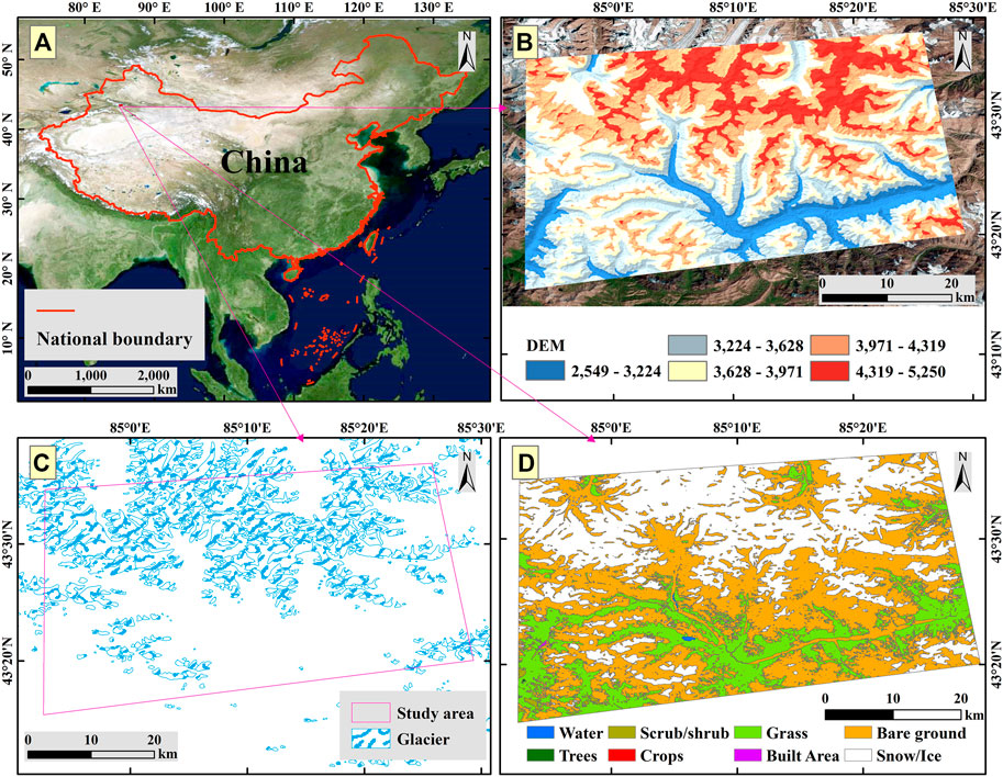
FIGURE 1. Overview map of the study area [(A) location of study area in China; (B) digital elevation model (DEM) of the study area; (C) distribution of glaciers within the study area; (D) surface land cover of the study area derived from the Esri 2020 Global Land Cover dataset (Karra et al., 2021)].
The amount of thawing of snow cover and ice affects the succession and growth of the local grassland ecosystem (Du et al., 2020b), which has a significant influence on the standard of living of pastoralists living in this area. Snow cover and ice are also a source of water resource recharge for many rivers in the adjacent low-altitude areas, and their phase behavior change is a guarantee of water supply for people living and working downstream along the rivers. As global warming accelerates the thawing of snow and ice (Qin et al., 2018), the exposed subsurface land will accelerate subsidence of the regional ground surface. Excessive melting in till sedimentation (moraine) can alter local topography, thereby affecting regional runoff and the water cycle. The amount of surface subsidence or uplift is also related to the frequency of natural disasters such as landslides, collapses, and debris flows.
Du et al. (2021b) obtained deformation information from the open-pit mining zone in the lower right corner of the study area (43.28–43.35°N, 84.95–85.12°E) using the SBAS-InSAR technique and compared the results with field GNSS monitoring data. This effort demonstrated the outstanding measurement capability of SBAS-InSAR in this region and obtained credible results. Based on this work, the parameters involved in the SBAS-InSAR processing for this paper were consistent with their settings in the literature (Mora et al., 2002; Hu et al., 2021a; Du et al., 2021b; Kursah et al., 2021), ensuring the reliability of the results, and therefore it was unnecessary to verify the accuracy of the measurement results in this study. This paper focuses on obtaining surface settlement information through SBAS-InSAR processing and analyzing settlement or uplift characteristics to understand the deformation features of the study area over a 3-year period, which will provide basic data for regional development policy formulation. The obtained surface deformation information can be used as an input risk assessment dataset for natural disasters and other studies, thus offering great significance and usefulness.
Dataset and Methodology
Dataset
The 89-scene of Sentinel-1A ascending (satellite travelling south to north) acquisitions from December 25, 2017 to January 2, 2021 were downloaded from the ASF website (https://vertex.daac.asfalaska.edu/), along with the precise orbital data corresponding to each acquisition as obtained from the ESA website (https://qc.sentinel1.eo.esa.int/). In general, long-wavelength (low-frequency) bands have good long-range performance and easy access to high-power transmitters and huge antennas (Ferretti et al., 2007). Short-wavelength (high-frequency) bands generally give precise distances and positions, but have a short range of action (Liu et al., 2019). Sentinel-1A has been acquiring data since October 2014 and Sentinel-1B since September 2016 with c-band (4–8 GHz) (Zhu et al., 2019), which has some penetration while maintaining good monitoring capability (high spatial accuracy). Each sentinel-1 constellation is in a near-polar, sun-synchronous orbit, with a 12-day repeat cycle and the two-satellite constellation offers a 6-day repeat cycle, which ensures excellent monitoring capability (high temporal resolution). They are very commonly used as SAR image data and are free and open-source, with multiple modes (Stripmap, SM; Interferometric Wide swath, IW; Extra Wide swath, EW; Wave, WV) and multi-polarization (HH, VV, HH + HV, VV + VH) (Yang et al., 2015).
The data used in this paper were the single-look complex (SLC) Level 1 product in IW mode, which acquires 250 km of surface data at a spatial resolution of 5 × 20 m (single scene) (Yang et al., 2015) and contains both phase and amplitude information. Phase is a function of time, and distance measurements can be obtained based on phase and velocity information (Liu et al., 2019). Based on this, SAR images can be used for distance measurement and deformation observation (Ye, 2010; Hu et al., 2021b). To reduce the time spent on data processing, only the extent of images containing the study area was selected for processing in this paper.
DEM data were provided by the Shuttle Radar Topography Mission (SRTM) 1 Arc-Second Global DEM from the USGS Earth Explorer website (https://earthexplorer.usgs.gov/) with a spatial resolution of 30 m, which can be used to produce aspect and slope dataset products (Figure 2) and extract contour lines. Glacier distribution data were derived from the Second Glacier Inventory of China, which can be obtained from the National Tibetan Plateau/Third Pole Environment Data Center (TPDC) (https://data.tpdc.ac.cn/) in vector format.
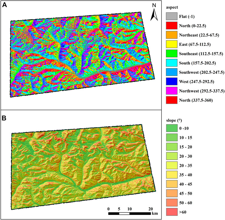
FIGURE 2. Ground surface topographical information of study area [(A) shows the aspect information and (B) is the slope data, and all are produced from the DEM dataset].
A ground-surface land coverage dataset (Figure 1D), Esri 2020 Global Land Cover (Karra et al., 2021) is based on the dataset produced for the Dynamic World Project by National Geographic Society in partnership with Google and the World Resources Institute. The map is derived from ESA Sentinel-2 imagery at 10 m resolution. It is a composite of LULC predictions for 10 classes throughout the year in order to generate a representative snapshot of 2020 and was produced by a deep learning model trained using over five billion hand-labeled Sentinel-2 pixels, sampled from over 20,000 sites distributed across all major biomes of the world. This dataset is now officially available for global public access and can be downloaded freely through the Land Cover Downloader Map website page (https://www.arcgis.com/apps/instant/media/index.html?appid=fc92d38533d440078f17678ebc20e8e2 or https://ai4edataeuwest.blob.core.windows.net/io-lulc/io-lulc-model-001-v01-composite-v03-supercell-v02-clip-v01.zip). Compared to FROM-GLC10 dataset (Gong et al., 2019), Esri 2020 Global Land Cover is closer to the date of acquisition of the SAR images (December 25, 2017 to January 2, 2021) of the study area and has a higher accuracy of ground features classification.
SBAS-InSAR
Since its introduction in 2002 (Mora et al., 2002), SBAS-InSAR technology has been used in many surface deformation monitoring studies. The principles, processing procedures, and other features of SBAS-InSAR have been extensively described in the literature (A. J. Hooper, 2008; Liu et al., 2019; Hu et al., 2021b) and will not be repeated in this paper. In this study, the SBAS-InSAR process was implemented on the SARscape 5.2.1 software platform, and its parameter settings and process were consistent with those in the literature (Chen et al., 2013; Du and Zhao, 2020; Reinosch et al., 2020; Du et al., 2021a; Du et al., 2021b; Du et al., 2021d). Table 1 gives the parameter settings of each step.
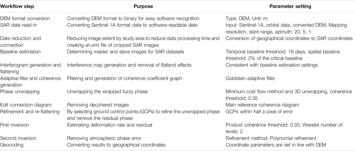
TABLE 1. Main purposes and parameter settings of SBAS-InSAR workflow steps.
The annual rate (mm/a) for the study area during the 3-year period from December 25, 2017 to January 2, 2021 and the surface cumulative deformation information (mm) will be available once the SBAS-InSAR processing has been completed. Deformation includes subsidence and uplift and represents cumulative deformation information describing ground surface changes for each relevant period starting on December 25, 2017 and ending with the date of image acquisition. Many important intermediate files used during processing will also be available, such as the coherence coefficient graphs, deformation maps of the first estimate, deformation maps after the second estimate, and other important reference files. In the InSAR process, the coherence coefficient is an important parameter ranging from 0 to 1 that determines the accuracy of the measurement results. The magnitude of the coherence coefficient indicates the extent of decohered, and the coherence coefficient can also be used as a threshold to remove low-coherence areas to improve the accuracy of the monitoring results.
Generally, if the coherence is less than 0.2 (Liu et al., 2019; Hu et al., 2021b), there may be few decohered regions, but the accuracy of the measurement results will be reduced. The coherence threshold will mask the areas where the coherence is less than the threshold value. Masked regions will be shown as blank in the result maps. In this study, the threshold was set to 0.35 to ensure the precision of the results.
Deformation Characterization
Deformation velocity maps and cumulative deformation maps were analyzed using the ArcGIS 10.6 software platform to identify the spatial and temporal deformation variation characteristics of the study region, focusing on the consistency and heterogeneity of the study area at overall and local scales. Regions with intense subsidence or uplift changes within the study area were analyzed and zoned in detail, and a set of observation points (OPs) was selected to extract the cumulative deformation for every period. Based on the Land Cover dataset, we have statistically analyzed the surface deformation characteristics of each type of ground feature, including the velocity range, decohered area, and decohered area percentage. This involved reclassifying the deformation velocity and transforming the raster results to vector format to extract the areas of each class, followed by reanalysis and counting of the land-cover area in each class.
The Raster to Point tool was used to transfer the acquired deformation velocity result to vector format points which were used as a baseline to extract other corresponding values including slope, aspect, elevation, and surface feature using the Extract Values to Points tool. The velocity map can also be transferred to vector polygon for area calculation using the Raster to Polygon tool. However, as the Raster to Polygon tool only supports data in integer, it is necessary to convert the results of the data type float to integer before raster to polygon processing. The extraction and processing of the relevant data corresponding to each ground cover data is similar.
The overlay method was used to analyze the relationship between deformation and land cover, as well as to collect deformation information for each land-cover type. More attention was paid to areas with intense variation and steep slopes to explore the intrinsic relevance between them. Slope data were obtained by calculating the DEM.
During the analysis, all the processes just described were not separate, but rather intertwined with each other. These analyses provided an understanding of the ground surface change characteristics of the study area and a preliminary analysis of deformation factors. The results provide a theoretical basis for formulating regional development policies as well as basic data for physical geological hazard prevention.
Results
Deformation Velocity and Cumulative Deformation
A velocity map (Figure 3) and cumulative deformation maps (Figures 5–7) for the 3 years were created once SBAS-InSAR processing had been completed. Warm colors indicate surface deformation away from the sensor line-of-sight (LOS) direction, whereas cool colors indicate surface deformation toward the sensor LOS direction. Blank regions represent missing data due to decohered. All the deformation descriptions information including the uplift and subsidence about the velocity and cumulative deformation in this paper are based on the sensor (LOS) direction.
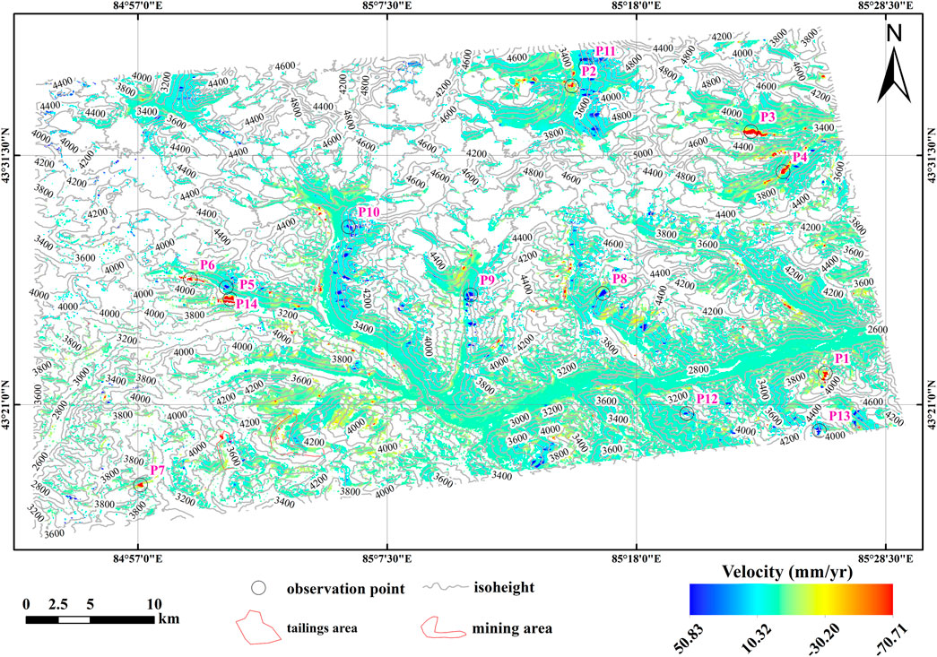
FIGURE 3. Deformation velocity of the study area. 14 observation points were selected in areas of intensity deformation. An open-pit mining site is located in the southwest section (84.95–85.12°E and 43.28–43.35°N).
Figure 3 shows regions of significant subsidence in the northeastern, southwestern, and southeastern sections of the study area, with rates of subsidence of −30.2 mm/a or more. The northern, central, and southern parts of the study area contain regions of significant uplift, with uplift rates greater than 15.6 mm/a. Areas with obvious deformation are isolated and sporadic. In the southwestern section, there is an open-pit mine, where Du et al. (2021b) have analyzed the associated ground deformation and obtained results in accord with the velocity results comparing with the situ global navigation satellite system (GNSS) measurements. The processing and parameter settings in this paper are identical to those of the literature (Du et al., 2021b), which ensures the reliability and scientific validity of the SBAS-InSAR measurements results in this paper. The maximum settlement rate in the study area was −71.7 mm/a, and the maximum uplift rate was 50.8 mm/a. Settlement rates in other valuable areas mostly ranged from −15.4 to 15.6 mm/a (Figure 4).
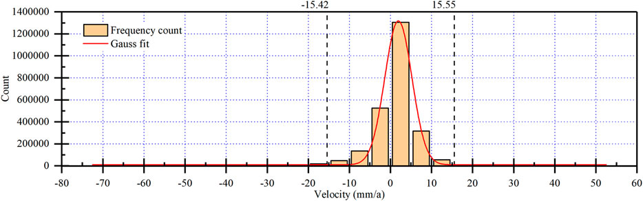
FIGURE 4. Deformation velocity statistics in the study area. All the velocity values are obtained by applying the Raster to point tool based on the velocity raster data.
The areas of cumulative deformation change in 2018 are concentrated at P11, P10, P9, and P8 (marked with small rectangles, pentagrams, ellipses, and large rectangles respectively in Figure 5, respectively). All four sites are in the subsidence zone and the changes are mainly reflected in an increase in the area of subsidence and an acceleration of subsidence rate. However, there are also some seasonal fluctuations, with an increase in subsidence from January to June and a slowdown in subsidence from June to December. The reason for this phenomenon may be due to the lifting of the ground surface caused by freeze-thaw action.
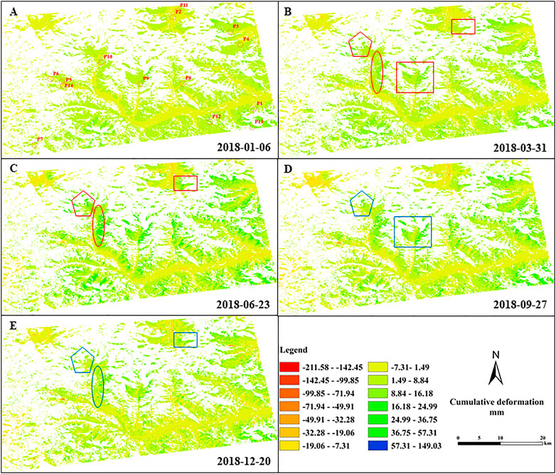
FIGURE 5. Cumulative deformation (mm) during 2018 [(A–F) are the dates of 2018-01-06, 2018-03-31, 2018-06-23, 2018-09-27, and 2018-1220, respectively]. The small red circles in (A) show the areas with evident deformation rate (14 observations). Other geometric labels indicate areas of significant change, with red indicating subsidence and blue indicating uplift.
The change from 2018 to 2019 is most evident at P14, P12, P9, and P13, (marked with a triangle, large ellipses, small ellipses, and large circle on Figure 6, respectively). By January 1, 2019, subsidence at P14 continued to increase until December 27, 2019 and had expanded in area. Other regional changes were characterized by similar cyclical fluctuations as in 2018. However, between June 30, 2019 and September 22, 2019, small landslides occurred in P13, P9, and the south-central section through the investigation of historical imageries and information, resulting in greater subsidence during this period, shown as a number of small dark blue dots in Figure 6. By the end of 2019, deformation in these three regions had stabilized.
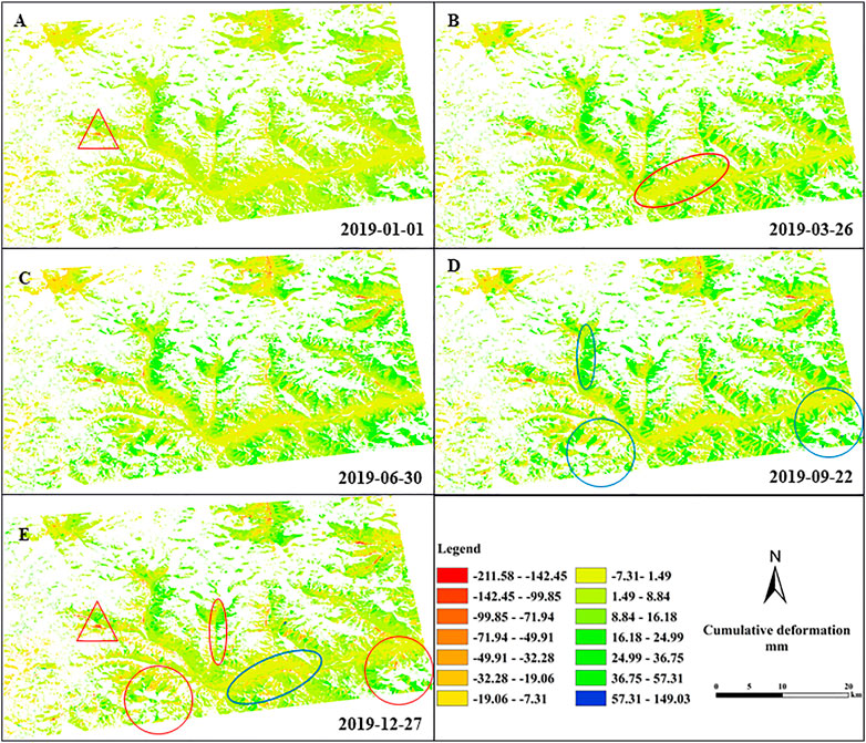
FIGURE 6. Cumulative deformation (mm) during 2019 [(A–F) are the dates of 2019–01-01, 2019-03–26, 2019-06–30, 2019-09–22, and 2019-12–27, respectively]. Geometric labels indicate areas of significant change, with red indicating subsidence and blue indicating uplift.
Changes in 2019 are mainly in P14 (marked by a red triangle on Figure 7), with continued subsidence and an increase in the area of subsidence. Other areas show little change, mainly due to cyclical variations caused by freeze-thaw action. However, due to landslides during 2018 in P13, P9 and the south-central region, freeze-thaw uplift caused by loose accumulation is greater than that in the past and is shown on the map as a more concentrated darker area (marked with blue ovals and circles on Figure 7, respectively).
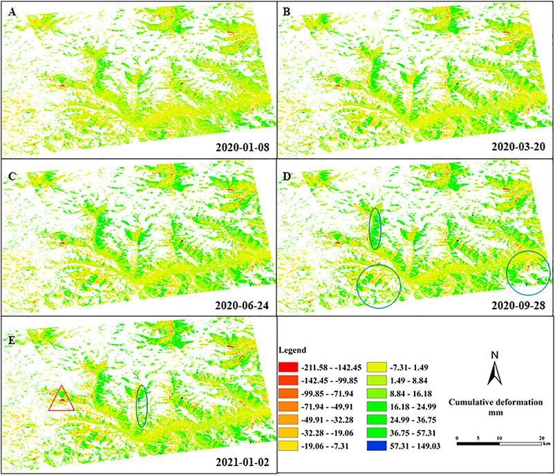
FIGURE 7. Cumulative deformation (mm) during 2020 [(A–F) are the dates of 2020–01-08, 2020-03–20, 2020-06–24, 2020-09–28, and 2021-01–02, respectively]. Geometric labels indicate areas of significant change, with red indicating subsidence and blue indicating uplift.
From Figures 5–7, we find that the cumulative deformation for each period was based on the starting date of December 25, 2017 and ended with the SAR image acquisition date. It is obvious that as time goes by, the cumulative deformation of the area near P14 (marked with a red triangle in Figures 6, 7) becomes larger. From January 6, 2018 to December 20, 2018, the maximum uplift varied from 26.80 to 50.47 mm, with a growth rate of 88.32%. The maximum settlement varied from −28.15 to −65.73 mm, with an added value up to 37.58 mm. In 2019, the added values of uplift and settlement were 48.29 and 66.41 mm, with growth rates of 93.01 and 96.38%, respectively. In 2020, uplift varied from 102.23 to 149.03 mm, representing an addition of 46.8 mm, and settlement changed from −137.69 to −211.58 mm, with a 53.67% growth rate.
According to velocity maps (Figure 2) and cumulative deformation graphs (Figures 5–7), the regions with violent settlement or uplift are relatively scattered. Settlement regions are distributed in the northeast, southwest, and southeast sections of the study area, whereas uplift is obvious in the north and central areas. All these zones are isolated and sporadic.
Area Statistics and Quantitative Analysis
In order to understand the deformation characteristics corresponding to each land cover type, we took the land cover raster dataset as a baseline and converted it to vector data using the Raster to Polygon tool. The vector data were then used to calculate the area of each ground land cover and the area of decohered regions (blank area in Figures 3, 5–7). Statistical indicators were calculated for each land cover, including the proportion of decohered area, velocity range, mean, media number, and standard deviation (SD). The results are shown in Table 2.
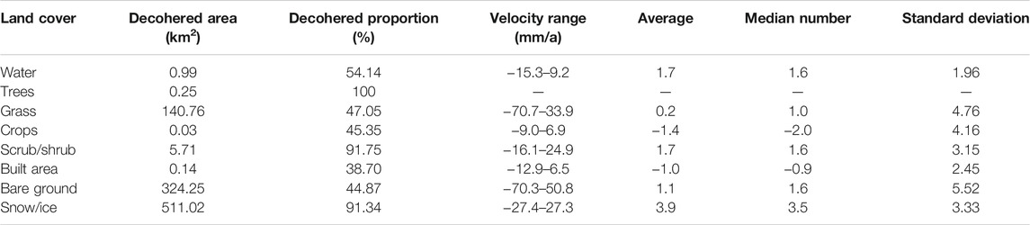
TABLE 2. Statistics on deformation velocities corresponding to different land covers.
After the calculation,the entire area of the entire research region is 1,590.78 km2. Bare ground occupied the largest area with 772.63 km2 or 45.45%. This is followed by snow/ice and grass with 35.18% (559.47 km2) and 18.82% (299.21 km2), respectively. The other 0.55% were scrub/shrub (6.23 km2), water (1.83 km2), built-up areas (0.35 km2), trees (0.25 km2), and crops (0.06 km2) respectively. From Table 2 and statistical calculations, the results indicate that the decohered phenomenon is serious within the entire study area, with the area of decorrelation being 984.11 km2 and accounting for 61.87% of total area. The effective measurement area is only 38.13%, with an area of 606.67 km2. And bare ground, grass, and snow/ice are 398.38, 158.44, and 48.45 km2, respectively. The areas of other land cover types are all less than 0.6 km2.
Of the eight land cover types from Table 2, bare ground has the greatest range of velocity variation at −70.3–50.8 mm/a and crops have the smallest range of velocity variation at −9.0–6.9 mm/a. This result is due to the large area of bare ground and landslides occurring within. The area of crops is small and does not vary much. The settlement rate of grassland is significantly greater than the uplift rate, which is due to the fact that part of the area where the landslide is close to grassland, resulting in an increase in the settlement rate of grassland. Snow/ice deformation rates ranged from −27.4–27.2 mm/a relatively symmetrically, with sedimentation rates slightly greater than uplift rates due to seasonal freeze-thaw. But the mean and median rates are positive, indicating the presence of localised widespread subsidence at snow/ice. Scrub/shrub rates varied mainly due to environmental succession caused by seasonal freeze-thaw and snow/ice thawing, ranging from −16.1–24.9 mm/a with an average rate of 1.7 mm/a.
The built area is dominated by a subsidence trend with an average rate of −1.0 mm/a, mainly due to the thawing of the ground ice and permafrost, and more care should be taken to prevent the risk of collapse in the future. Water changes are somewhat fortuitous and the results are not very meaningful. The region of trees is completely decohered and cannot be effectively monitored for surface deformation.
The statistical analysis revealed that the study area was severely decohered. The severity of the decorrelation was found to be in trees, scrub/shrub, snow/ice, water, grass, crops, bare ground, and built area with the area decohered proportion of 100, 91.75, 91.34, 54.14, 47.05, 45.35, 44.87, and 38.7%, respectively.
Time-Series Variation Characteristics of Cumulative Deformation
To determine the variation characteristics of cumulative deformation, 14 observation points (OPs) (Table 3, Figures 3, 6A) were selected in areas with dramatic variation, and the cumulative deformation was extracted for each point. Figure 8 shows the results.
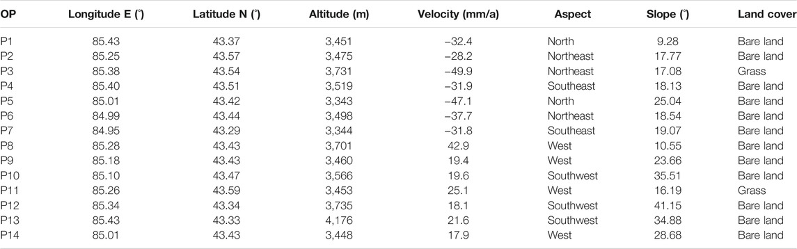
TABLE 3. Basic information for the observation points.
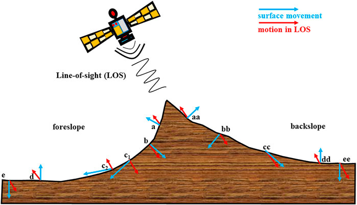
FIGURE 8. The relationship between surface movements and InSAR detected displacements in LOS direction, particularly for mountainous regions, derived from literature (Chen et al., 2013).
Due to the posture limitations of the SAR satellite when observing, the deformation information obtained through InSAR processing is usually not the real deformation of surface ground, instead the LOS direction. The effectiveness of the deformation results obtained is closely related to the terrain (slope and aspect) (see Figure 8), especially in mountainous areas. Specifically, with a few exceptions, the direction of surface movements fits expectations: the parallel movement, caused by widespread slope processes (e.g., general creep), was dominant in the middle section of slopes; for other portions, the rotational motion was prevalently caused by the alluvial accumulation or the combination dynamics of permafrost and the overlaid active layer (Chen et al., 2013). In addition, the occurrence of landslide will form a serious deformation area in a short time.
Figure 8 shows a high agreement between the real surface deformation and the motion in the LOS direction, both at the top of the mountain and at the foot of the mountain, fore and back the slope (a, aa, b, bb, c1, cc, d, dd, e, and ee in Figure 8). Ground heave shows as uplift in LOS and surface settlement as subsidence in LOS. It is only when the slope faces satellite and slope gradient is greater than satellite incidence angle that the inconsistency is shown. In Figure 8, c2 marks a slope process (blue line), and an uplift signal is manifested in the LOS direction (red line).
The incidence angle of Sentinel-1A images used in this study is 39.08°. For ascending orbit, the west aspect is the satellite-facing slope and the east aspect is the satellite-away slope (Schaufler et al., 2018). Combining the slope and aspect dataset (Figure 2), the deformation velocity map (Figure 3), and the slope-velocity and aspect-velocity statistics (Figures 11A,B), we recognize that most uplift signals are located on satellite-facing slopes (west) and extensive subsidence signals are located on the east aspect. The signals (uplift and subsidence) are more likely caused by slope processes/land sliding.
To further understand the relationship between deformation rate and slope, slope orientation and vegetation, we counted the percentage of each element in the area with deformation rate greater than 15.0 mm/a. The results showed that, except for trees, the deformation rates of bare ground, grassland, snow, and wetland were all greater than 15.0 mm/a among the remaining seven types of ground features, with the percentages of 75.99, 17.91, 5.98, and 0.12%, respectively, and the deformation rates were concentrated between 16.0 and 21.5 mm/a. More statistical information is shown in Table 4.
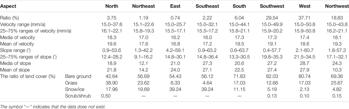
TABLE 4. Characteristic statistics of areas with the deformation rate greater than 15.0 mm/a.
It can be found from Table 4 that the areas with deformation velocity greater than 15.0 mm/a in the study area are mostly concentrated in the west, southwest, and northwest sides of the slope direction, accounting for 37.71, 29.54, and 18.83%, respectively. The west aspect is the satellite-facing slope and ascending orbits show a positive shift in backscatter for slopes facing west (Schaufler et al., 2018), so that the landslide accumulation phenomenon can be well observed in this area. Moreover, the slope of the hills sloping to the west is also relatively large, concentrated between 17.1 and 35.3°, and the average slope is all greater than 24.3°. In addition, the area is mostly covered with bare land, followed by grassland, with little snow/ice and scrub/shrub coverage, which is more likely to cause landslides and should be paid special attention.
The cumulative deformation of the OPs shows that points P1–P7 are situated in a settlement area, whereas P9–P14 are situated in an uplift area. Over time, the cumulative deformation becomes greater, involving both settlement and uplift. The slope of the cumulative deformation curves shows the velocity of deformation, and P3 and P8 have the maximum values of settlement and uplift, respectively, which agrees with the velocities in Table 3. Compared with settlement curves, uplift curves show more volatility, especially those for P13 and P14. However, some anomalies were observed in settlement curves, such as P2 on August 22, 2018 and September 16, 2019 and P7 on April 19, 2019. The sudden jumps that appeared in Figure 9 were very likely due to unwrapping errors or other noises.
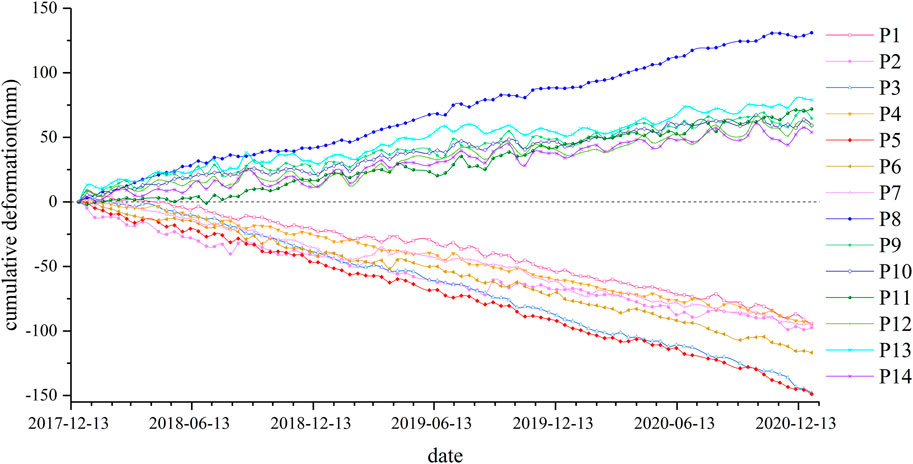
FIGURE 9. Cumulative deformation (mm) of the observation points. And P1-P7 (cool color), P8-P14 (warm color) are uplift and subside toward the LOS direction, respectively. Slope of the curve shows the deformation velocity (mm/a).
By investigating historical imagery data, mainly via comparing Esri satellite maps and Google searching historical images, we found that the location where P7 is located originally had significant amounts of snow cover and ice, which has now largely thawed with global warming (Figure 10). The seasonal freezing and thawing of snow cover and ice, as well as the effects of solid winter precipitation, have induced small seasonal fluctuations changes in the cumulative deformation chart at point P7, but the overall trend is settlement.
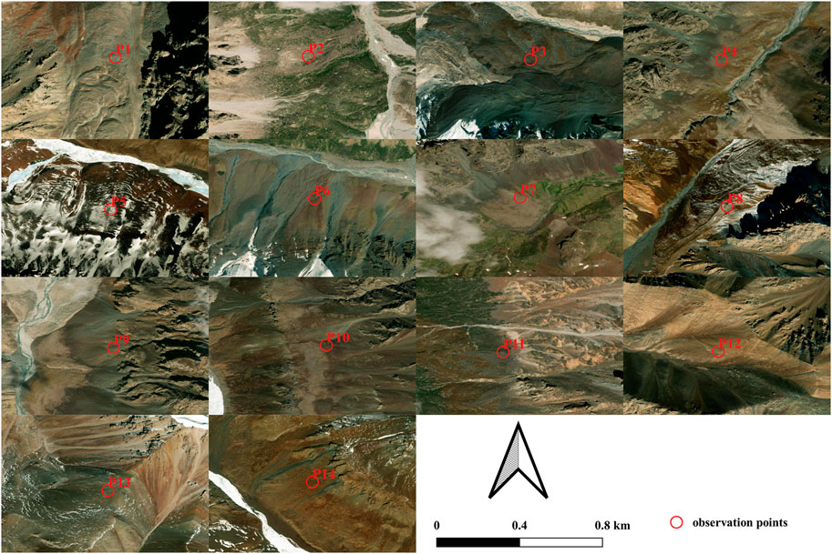
FIGURE 10. The close-up shots around the observation points based on Esri satellite image maps on a scale of 1:380,000.
According to close-up shots of the 14 OPs based on Esri satellite image maps (Figure 9), the settlement areas are mostly at the foot of mountains, which have an abundance of broken rocks or areas covered with snow and ice, especially on steep ridges where the landslides are prone to occur. Uplift regions occur mostly in the basins between ridges with relatively flat terrain, near the runoff points, so that changes in river discharge may modify the cumulative deformation process.
Relationship Between Deformation and Topographical Elements
Raster to Point tool was used to create the monitoring points (MPs) consistent with the deformation velocity raster grids within the area and extract the velocity, DEM, aspect, and slope of each point. Aspect and slope dataset for the study area (Figure 2) were produced from DEM data. Decohered areas without a deformation rate were rejected, and a total of 242,778 points were generated.
The statistical analysis addressed the distribution of effective MPs and the relationships between velocity and aspect, slope, and elevation. The results are shown in Figure 11. Most of the MPs are distributed in the areas toward the southeast, south, and southwest (112.5–247.5), with slopes ranging from 15° to 50° and altitudes ranging from 3,150 m.a.s.l. to 4,275 m.a.s.l. MPs are less prevalent in areas with slopes greater than 60° and altitudes higher than 4,275 m.
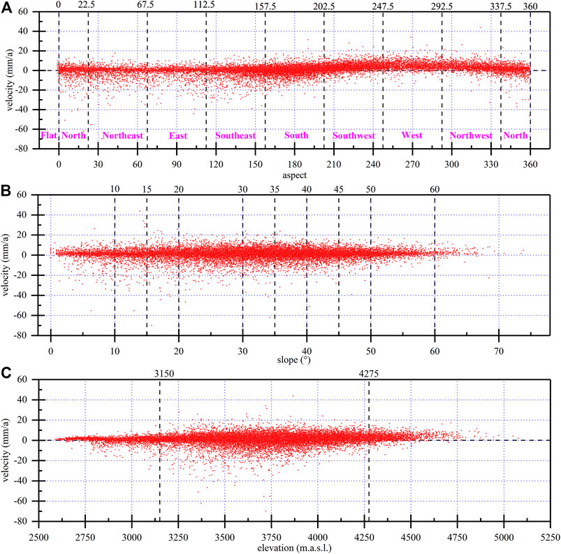
FIGURE 11. Statistical distribution of terrain factors and deformation [(A,B,C) show the relationship between aspect, slope, and elevation, respectively].
Therefore, most of the deformation occurs in areas with slopes of 15–50° and elevations of 3,150–4,275 m.a.s.l., especially in regions with southwest, west, and northwest aspects. Ground areas with severe deformation may induce some secondary geological disasters, such as landslides, collapses, and mud-rock flows.
Discussion
Due to the inherent limitations of InSAR measurements, certain areas lack deformation data due to decorrelation. In this study, significant incoherent regions covered with glaciers, snow cover, and ice were observed within the study area. In addition to the shortcomings of InSAR itself, this phenomenon is also related to the fact that degeneration of glaciers and snow cover not only occurs abruptly, but also in large amounts. Effective solutions for areas with missing values include field surveys, which can then be supplemented by spatial interpolation (Zhang, 2010). Alternatively, InSAR measurements can be processed from multiple SAR image sources and the results combined (Wang, 2019; Zhu et al., 2019). Sources of SAR images include products taken by different sensors, at different orientations, or in different time periods. In addition, reducing the coherence threshold is an effective method.
The deformation data obtained are of great significance, despite the large number of decoherent zones in the study area. The measurement results can provide basic advice and information for later continuous observations, and use of a sequential adjustment method (Wang et al., 2021) ensures that the long time series of SBAS-InSAR measurement data can be supplemented at a later stage. At the same time, current deformation values can provide a theoretical basis for environmental development by the local government. More importantly, the deformation data can provide a general picture over large areas and long time series of the distribution of mines and the degeneration of snow cover and ice in the area.
There are some differences regarding land cover between the close-up shots of OPs P5–P7 in Figure 9 and the land-cover data in Table 3; these may have been caused by the different dates of the images obtained. Land-cover data is derived from ESA Sentinel-2 imagery at 10 m resolution. And it is a composite of LULC predictions for 10 classes throughout the year in order to generate a representative snapshot of 2020. Whereas the close-up shots were based on the 2020 Esri image maps, which were the integrated product of various satellite images.
The question of whether the deformation in the LOS direction reflects the true displacement of the ground surface has been addressed in many papers (Chen et al., 2013; Liu et al., 2019; Hu et al., 2021b; Ge et al., 2021). As the monitoring results in this paper are obtained based on a single data source and a single InSAR processing method, it is difficult to obtain the real 3-D ground surface deformation. However, combining the available relevant theories (Chen et al., 2013; Reinosch et al., 2020) and the geometric relationship between SAR satellites and monitoring sites (mainly concerning slope and aspect), we found that there are almost no anomalies (the deformation in the LOS direction does not coincide with the true surface displacement) in this study area and the deformation values of the monitoring points are highly consistent with the real surface displacement. The reliability of results in this paper is also supported by the high agreement between the InSAR deformation monitoring values and the actual monitoring values for the mine sites located within the study area (Du et al., 2021b). The correlation between slope and deformation velocity needs to be investigated in depth in the follow-up to propose slope threshold of slope when the anomalies occurred, which will allow us to better analyze the real surface displacements.
Conclusion
1) The maximum subsidence velocity in the study area was -70.7 mm/a in the western, northeastern, and southeastern regions, and the maximum uplift rate was 50.8 mm/a in the northern and central regions. The areas with intense subsidence and uplift were isolated and sporadic.
2) The maximum cumulative subsidence in the study area for the 3-year period from December 25, 2017 to January 2, 2021 was −211.58 mm, and the maximum cumulative uplift was 149.03 mm, which was consistent with the deformation velocity.
3) The study area was severely decohered, with a decorrelation area of 984.11 km2, accounting for 61.87% of the total area. The severity of the decorrelation is trees, scrub/shrub, snow/ice, water, grass, crops, bare ground and built area,with decohered percentage of own area 100, 91.75, 91.34, 54.14, 47.05, 45.35, 44.87, and 38.7%, respectively.
4) There were correlations between deformation and slope, slope direction, and elevation. Specifically, deformation was obvious in areas with elevations between 3,150 and 4,275 m.a.s.l., slopes of 15°–50°, and southwest, west, and northwest aspects, which are disaster-prone regions.
Data Availability Statement
The original contributions presented in the study are included in the article/supplementary material, further inquiries can be directed to the corresponding author.
Author Contributions
QD and GL conceived this research. QD prepared the data and wrote the manuscript. All other co-authors reviewed and supervised the manuscript and all authors listed approved it for publication.
Funding
This study was funded by the National Natural Science Foundation of China (No. U1703244), the Second Tibetan Plateau Scientific Expedition and Research Program (No.2019QZKK0905), the Foundation of the State Key Laboratory of Frozen Soil Engineering (No. SKLFSE-ZY-20), the Foundation of the State Key Laboratory for Geomechanics and Deep Underground Engineering (No. SKLGDUEK 1904).
Conflict of Interest
The authors declare that the research was conducted in the absence of any commercial or financial relationships that could be construed as a potential conflict of interest.
Publisher’s Note
All claims expressed in this article are solely those of the authors and do not necessarily represent those of their affiliated organizations, or those of the publisher, the editors and the reviewers. Any product that may be evaluated in this article, or claim that may be made by its manufacturer, is not guaranteed or endorsed by the publisher.
Acknowledgments
Thanks to the teams of organizations and individuals for providing the open and free source data involved in this paper. We express our deepest gratitude to the reviewers, whose careful work and thoughtful suggestions have greatly helped to improve this paper substantially.
References
Amelung, F., Galloway, D. L., Bell, J. W., Zebker, H. A., and Laczniak, R. J. (1999). Sensing the Ups and Downs of Las Vegas: InSAR Reveals Structural Control of Land Subsidence and Aquifer-System Deformation. Geology 27 (6), 483–486. doi:10.1130/0091-7613(1999)027<0483:STUADO>2.3.CO;2
Bamler, R., and Hartl, P. (2010). Synthetic Aperture Radar Interferometry. Sci. Geodesy - Adv. Future Dir. 1, 415–474. doi:10.1007/978-3-642-11741-1_11
Chen, F., Lin, H., Zhou, W., Hong, T., and Wang, G. (2013). Surface Deformation Detected by ALOS PALSAR Small Baseline SAR Interferometry Over Permafrost Environment of Beiluhe Section, Tibet Plateau, China. Remote Sensing Environ. 138, 10–18. doi:10.1016/j.rse.2013.07.006
Cheng, G., Zhao, L., Li, R., Wu, X., Sheng, Y., Hu, G., et al. (2019). Characteristic, Changes and Impacts of Permafrost on Qinghai-Tibet Plateau. Chin. Sci. Bull. 64 (27), 2783–2795. doi:10.1360/TB-2019-0191
Colesanti, C., Ferretti, A., Prati, C., and Rocca, F. (2003). Monitoring Landslides and Tectonic Motions with the Permanent Scatterers Technique. Eng. Geology. 68 (1–2), 3–14. doi:10.1016/S0013-7952(02)00195-3
Du, Q., Li, G., Li, J., and Zhou, Y. (2020a). Research on the River Extration Based on the DEM Data in the Centeral West Tianshan Mountains. China Rural Water and Hydropower 456 (10), 29–33+40.
Du, Q., Li, G., Peng, W., Chai, M., Zhou, Y., and Chen, D. (2020b). Land Use Changes in High Cold-Altitude Mining Area Based on Remote Sensing Technology. Environ. Sci. Technol. 43 (12), 185–194. doi:10.19672/j.cnki.1003-6504.2020.12.025
Du, Q., Li, G., Peng, W., Zhou, Y., Chai, M., and Li, J. (2021a). Acquiring High-Precision DEM in High Altitude and Cold Area Using InSAR Technology. Bull. Surv. Mapp. 528 (03), 44–49. doi:10.13474/j.cnki.11-2246.2021.0076
Du, Q., Li, G., Zhou, Y., Chai, M., Chen, D., Qi, S., et al. (2021b). Deformation Monitoring in an Alpine Mining Area in the Tianshan Mountains Based on SBAS-InSAR Technology. Adv. Mater. Sci. Eng. 2021, 1–15. doi:10.1155/2021/9988017
Du, Q., Li, G., Zhou, Y., Wu, G., Chai, M., and Li, F. (2021c). Distribution Characterization Study of the Heavy Metals for a Mining Area of East Tianshan Mountain in Xinjiang Based on the Kriging Interpolation Method. IOP Conf. Ser. Earth Environ. Sci. 719 (4), 042063. doi:10.1088/1755-1315/719/4/042063
Du, Q., and Zhao, R. (2020). The Production of DEM in SARscape Format. Comput. Knowledge Technol. 16 (07), 238–239. doi:10.14004/j.cnki.ckt.2020.0838
Du, Y., Yan, S., Yang, H., Jiang, J., and Zhao, F. (2021d). Investigation of Deformation Patterns by DS-InSAR in a Coal Resource-Exhausted Region with Spaceborne SAR Imagery. J. Asian Earth Sci. X 5, 100049. doi:10.1016/j.jaesx.2021.100049
Ferretti, A., Montiguarnieri, A., Prati, C., Rocca, F., and Massonet, D. (2007). InSAR Principles: Guidelines for SAR Interferometry Processing and Interpretation. J. Financial Stab. 10 (10), 156–162. doi:10.1287/ited.1100.0047
Ferretti, A., Prati, C., and Rocca, F. (2001). Permanent Scatterers in SAR Interferometry. IEEE Trans. Geosci. Remote Sensing 39 (1), 8–20. doi:10.1109/36.898661
Gatsios, T., Cigna, F., Tapete, D., Sakkas, V., Pavlou, K., and Parcharidis, I. (2020). Copernicus sentinel-1 MT-InSAR, GNSS and Seismic Monitoring of Deformation Patterns and Trends at the Methana Volcano, Greece. Appl. Sci. 10 (18), 6445–6523. doi:10.3390/APP10186445
Ge, W., Li, Y., Wang, Z., Zhang, C., and Yang, H. (2021). Spatial‐Temporal Ground Deformation Study of Baotou Based on the PS‐InSAR Method. Acta Geologica Sinica ‐ English Edition 95 (2), 674–683. doi:10.1111/1755-6724.14651
Gong, P., Liu, H., Zhang, M., Li, C., Wang, J., Huang, H., et al. (2019). Stable Classification with Limited Sample: Transferring a 30-m Resolution Sample Set Collected in 2015 to Mapping 10-m Resolution Global Land Cover in 2017. Sci. Bull. 64 (6), 370–373. doi:10.1016/j.scib.2019.03.002
Hanssen, R. F. (2001). Radar Interferometry Data Interpretation and Error Analysis. Dordrecht, Netherlands: Springer Science and Business Media.
Hanssen, R. F., Weckwerth, T. M., Zebker, H. A., and Klees, R. (1999). High-Resolution Water Vapor Mapping from Interferometric Radar Measurements. Science 283 (5406), 1297–1299. doi:10.1126/science.283.5406.1297
Hansson, A., Anshelm, J., Fridahl, M., and Haikola, S. (2021). Boundary Work and Interpretations in the IPCC Review Process of the Role of Bioenergy with Carbon Capture and Storage (BECCS) in Limiting Global Warming to 1.5°C. Front. Clim. 3, 1–14. doi:10.3389/fclim.2021.643224
He, M., and Zhao, Y. (2020). Study on the Application Prospect of DS-InSAR Technology in Landslide Deformation Monitoring in Complex and Dangerous Mountainous Areas. Geomatics Sci. Technol. 08 (03), 106–113. doi:10.12677/gst.2020.83013
Hooper, A. (2008). A Multi-Temporal InSAR Method Incorporating Both Persistent Scatterer and Small Baseline Approaches. Geophys. Res. Lett. 35 (16), 1–5. doi:10.1029/2008GL034654
Hooper, A., Zebker, H., Segall, P., and Kampes, B. (2004). A New Method for Measuring Deformation on Volcanoes and Other Natural Terrains Using InSAR Persistent Scatterers. Geophys. Res. Lett. 31 (23), 1–5. doi:10.1029/2004GL021737
Hu, J., Ge, Q., Liu, J., Yang, W., Du, Z., and He, L. (2021a). Constructing Adaptive Deformation Models for Estimating DEM Error in SBAS-InSAR Based on Hypothesis Testing. Remote Sensing 13 (10), 2006. doi:10.3390/rs13102006
Hu, J., Li, Z., Zhu, J., and Liu, J. (2021b). Theory and Application of Monitoring 3-D Deformation with InSAR. Beijing, China: Science Press.
Karra, K., Kontgis, C., Statman-Weil, Z., Mazzariello, J., Mathis, M., and Brumby, S. (2021). “Global Land Use/land Cover with Sentinel-2 and Deep Learning,” in IGARSS 2021-2021 IEEE International Geoscience and Remote Sensing Symposium, Brussels, Belgium, June 11–July 16, 2021 (IEEE).
Kursah, M. B., Wang, Y., Bayoh, H. D., David Bayoh, H., Tarawally, M., and Leone, S. (2021). A Comparative Study on the Predictive Ability of Archived and SBAS-InSAR Inventories for Landslide Susceptibility Using Frequency Ratio Model in Western Area, Sierra Leone. Environ. Earth Sci. 80, 387. doi:10.1007/s12665-021-09663-x
Li, Q., Zhou, C., Zheng, L., Liu, T., and Yang, X. (2020). Monitoring Evolution of Melt Ponds on First- Year and Multiyear Sea Ice in the Canadian Arctic Archipelago with Optical Satellite Data. Ann. Glaciology 61 (82), 1–10. doi:10.1017/aog.2020.24
Liu, G., Chen, Q., Chen, X., and Cai, G. (2019). InSAR Principles and Applications. Beijing, China: Science Press.
Lu, Z., and Dzurisin, D. (2014). InSAR Imaging of Aleutian Volcanoes: Monitoring a Volcanic Arc from Space. Chichester, United Kingdom: Springer Praxis Books.
Massonnet, D., and Feigl, K. L. (1998). Radar Interferometry and its Application to Changes in the Earth's Surface. Rev. Geophys. 36 (4), 441–500. doi:10.1029/97RG03139
Metternicht, G., Hurni, L., and Gogu, R. (2005). Remote Sensing of Landslides: An Analysis of the Potential Contribution to Geo-Spatial Systems for hazard Assessment in Mountainous Environments. Remote Sensing Environ. 98 (2–3), 284–303. doi:10.1016/j.rse.2005.08.004
Monserrat, O., Crosetto, M., and Luzi, G. (2014). A Review of Ground-Based SAR Interferometry for Deformation Measurement. ISPRS J. Photogrammetry Remote Sensing 93, 40–48. doi:10.1016/j.isprsjprs.2014.04.001
Mora, O., Lanari, R., Mallorquí, J. J., Berardino, P., and Sansosti, E. (2002). “A New Algorithm for Monitoring Localized Deformation Phenomena Based on Small Baseline Differential SAR Interferograms,” in International Geoscience and Remote Sensing Symposium (IGARSS), Toronto, ON, June 24–28, 2002, 1237–1239. doi:10.1109/igarss.2002.1025900
Moreira, A., Prats-Iraola, P., Younis, M., Krieger, G., Hajnsek, I., and Papathanassiou, K. P. (2013). A Tutorial on Synthetic Aperture Radar. IEEE Geosci. Remote Sens. Mag. 1 (1), 6–43. doi:10.1109/MGRS.2013.2248301
Ouchi, K. (2013). Recent Trend and advance of Synthetic Aperture Radar with Selected Topics. Remote Sensing 5 (2), 716–807. doi:10.3390/rs5020716
Pepe, A., and Calò, F. (2017). A Review of Interferometric Synthetic Aperture RADAR (InSAR) Multi-Track Approaches for the Retrieval of Earth's Surface Displacements. Appl. Sci. 7 (12), 1264. doi:10.3390/app7121264
Qin, D., Yao, T., Ding, Y., and Ren, J. (2018). Introduction to Cryospheric Science. Beijing, China: Science Press.
Reinosch, E., Buckel, J., Dong, J., Gerke, M., Baade, J., and Riedel, B. (2020). InSAR Time Series Analysis of Seasonal Surface Displacement Dynamics on the Tibetan Plateau. The Cryosphere 14 (5), 1633–1650. doi:10.5194/tc-14-1633-2020
Rosen, P. A., Hensley, S., Joughin, I. R., Li, F. K., Madsen, S. N., Rodriguez, E., et al. (2000). Synthetic Aperture Radar Interferometry. Proc. IEEE 88 (3), 333–382. doi:10.1109/5.838084
Rott, H. (2009). Advances in Interferometric Synthetic Aperture Radar (InSAR) in Earth System Science. Prog. Phys. Geogr. Earth Environ. 33 (6), 769–791. doi:10.1177/0309133309350263
Schaufler, S., Bauer-Marschallinger, B., Hochstöger, S., and Wagner, W. (2018). Modelling and Correcting Azimuthal Anisotropy in sentinel-1 Backscatter Data. Remote Sensing Lett. 9 (8), 799–808. doi:10.1080/2150704X.2018.1480071
Shahzad, N., Ding, X., Wu, S., and Liang, H. (2020). Ground Deformation and its Causes in Abbottabad City, pakistan from sentinel-1a Data and Mt-Insar. Remote Sensing 12 (20), 1–18. doi:10.3390/rs12203442
Shan, W., Guo, Y., Zhang, C., Hu, Z., Jiang, H., and Wang, C. (2014). “Climate-Change Impacts on Embankments and Slope Stability in Permafrost Regions of Bei'an-Heihe Highway,” in Landslide Science for a Safer Geoenvironment. Editors K. Sassa, P. Canuti, and Y. Yin (London, United Kingdom: Springer International Publishing), 155–160. doi:10.1007/978-3-319-04999-1_18
Shan, W., Hu, Z., Guo, Y., Zhang, C., Wang, C., Jiang, H., et al. (2015). The Impact of Climate Change on Landslides in southeastern of High-Latitude Permafrost Regions of China. Front. Earth Sci. 3, 1–11. doi:10.3389/feart.2015.00007
Simons, M., and Rosen, P. A. (2007). Interferometric Synthetic Aperture Radar Geodesy. Treatise Geophys. 3, 391–446. doi:10.1016/B978-044452748-6.00059-6
Wang, H., Zeng, Q., Jiao, J., and Chen, J. (2021). InSAR Time Series Analysis Technique Combined with Sequential Adjustment Method for Monitoring of Surface Deformation. Beijing Daxue Xuebao (Ziran Kexue Ban)/Acta Scientiarum Naturalium Universitatis Pekinensis 57 (2), 241–249. doi:10.13209/j.0479-8023.2021.002
Wang, Z. (2019). Research on Resolving of Three-Dimensional Dispalcement from Multi-Source InSAR Data. Acta Geodaetica et Cartographica Sinica 48 (9), 1206. doi:10.11947/j.AGCS.2019.20180490
Yang, K., Yang, J., and Jiang, B. (2015). Sentinel-1 Satellite Overview. Urban Geotechnical Invest. Surv. 8262 (02), 24–27.
Ye, X. (2010). Synthetic Aperture Radar Interferometry. London, United Kingdom: Springer Berlin Heidelberg. doi:10.1007/978-3-642-11741-1
Zhang, J., Huang, H., Liu, Y., and Liu, Y. (2013). Monitoring and Analysis of Ground Subsidence in the Modern Yellow River Delta Area Based on PSInSAR Technique. Scientia Geographica Sinica 33 (07), 831–836. doi:10.13249/j.cnki.sgs.2013.07.008
Zhao, L., Hu, G., Zou, D., Wu, X., Ma, L., Sun, Z., et al. (2019). Permafrost Changes and its Effects on Hydrological Processes on Qinghai-Tibet Plateau. Bull. Chin. Acad. Sci. 34 (11), 1233–1246. doi:10.16418/j.issn.1000-3045.2019.11.006
Zhu, J., Yang, Z., and Li, Z. (2019). Recent Progress in Retrieving and Predicting Mining-Induced 3D Displacement Using InSAR. Acta Geodaetica et Cartographica Sinica 48 (02), 135–144. CNKI:SUN:CHXB.0.2019-02-002.
Zhu, L., Wu, Z., Liu, Y., and Li, D. (1996). Permafrost Degeneration in the East of Qinghai-Xizang Plateau. Chin. Geograph.Sc. 6 (3), 231–238. doi:10.1007/s11769-996-0025-2
Keywords: surface deformation, Eastern Tianshan Mountains, SBAS-InSAR, environmental impact, cold alpine and high-altitude regions, disaster prevention and mitigation
Citation: Du Q, Li G, Chen D, Zhou Y, Qi S, Wu G, Chai M, Tang L, Jia H and Peng W (2021) SBAS-InSAR-Based Analysis of Surface Deformation in the Eastern Tianshan Mountains, China. Front. Earth Sci. 9:729454. doi: 10.3389/feart.2021.729454
Received: 23 June 2021; Accepted: 30 September 2021;
Published: 03 November 2021.
Edited by:
Guo Donglin, Institute of Atmospheric Physics (CAS), ChinaReviewed by:
Wenyu Gong, China Earthquake Administration, ChinaWang Lingxiao, Nanjing University of Information Science and Technology, China
Copyright © 2021 Du, Li, Chen, Zhou, Qi, Wu, Chai, Tang, Jia and Peng. This is an open-access article distributed under the terms of the Creative Commons Attribution License (CC BY). The use, distribution or reproduction in other forums is permitted, provided the original author(s) and the copyright owner(s) are credited and that the original publication in this journal is cited, in accordance with accepted academic practice. No use, distribution or reproduction is permitted which does not comply with these terms.
*Correspondence: Guoyu Li, Z3VveXVsaUBsemIuYWMuY24=