 Qiang Wang
 Wei Zheng1,2,3*†
 Fan Wu
 Zongqiang Liu
- 1School of Geomatics, Liaoning Technical University, Fuxin, China
- 2Qian Xuesen Laboratory of Space Technology, China Academy of Space Technology, Beijing, China
- 3School of Astronautics, Taiyuan University of Technology, Jinzhong, China
- 4School of Astronautics, Nanjing University of Aeronautics and Astronautics, Nanjing, China
The global navigation satellite system reflectometer (GNSS-R) can improve the observation and inversion of mesoscale by increasing the spatial coverage of ocean surface observations. The traditional retracking method is an empirical model with lower accuracy and condenses the Delay-Doppler Map information to a single scalar metric cannot completely represent the sea surface height (SSH) information. Firstly, to use multi-dimensional inputs for SSH retrieval, this paper constructs a new machine learning weighted average fusion feature extraction method based on the machine learning fusion model and feature extraction, which takes airborne delay waveform (DW) data as input and SSH as output. R2-Ranking method is used for weighted fusion, and the weights are distributed by the coefficient of determination of cross validation on the training set. Moreover, based on the airborne delay waveform data set, three features that are sensitive to the height of the sea surface are constructed, including the delay of the 70% peak correlation power (PCP70), the waveform leading edge peak first derivative (PFD), and the leading edge slope (LES). The effect of feature sets with varying levels of information details are analyzed as well. Secondly, the global average sea surface DTU15, which has been corrected by tides, is used to verify the reliability of the new machine learning weighted average fusion feature extraction method. The results show that the best retrieval performance can be obtained by using DW, PCP70 and PFD features. Compared with the DTU15 model, the root mean square error is about 0.23 m, and the correlation coefficient is about 0.75. Thirdly, the retrieval performance of the new machine learning weighted average fusion feature extraction method and the traditional single-point re-tracking method are compared and analyzed. The results show that the new machine learning weighted average fusion feature extraction method can effectively improve the precision of SSH retrieval, in which the mean absolute error is reduced by 63.1 and 59.2% respectively, and the root mean square error is reduced by 63.3 and 61.8% respectively; The correlation coefficient increased by 31.6 and 44.2% respectively. This method will provide the theoretical method support for the future GNSS-R SSH altimetry verification satellite.
Introduction
Sea Surface Height (SSH), as an important ocean parameter, plays an important role in establishing global ocean tide models, observing large-scale ocean circulation, and monitoring global sea level changes (Zhang et al., 2020). Traditional spaceborne mono-static radar altimeters obtain marine physical parameter information by continuously transmitting radar pulses to the earth and receiving sea surface echoes, which have the disadvantages of low coverage, long repetition period, and high cost (Bosch et al., 2014; Zawadzki and Ablain 2016; Wang et al., 2021b). GNSS-R technology is an emerging remote sensing technology in sea surface altimetry in recent years. It is used to retrieve the sea surface height by measuring the time delay between the reflected signal and the direct signal. In 1993, the concept of Passive reflectometry and interferometry system was initially proposed by Martin-Neira, proving the capability of GNSS-R to ocean altimetry (Martin-Neira 1993). GNSS-R offers several advantages over mono-static radar systems including multiple measurements over a large area, reduced cost, reduced power consumption, all-weather and highly real-time (Mashburn et al., 2020). At present, this technology has been used for the detection of sea surface height (Mashburn et al., 2016; Mashburn et al. 2018; Mashburn et al. 2020), sea surface wind speed (Ruf et al., 2015; Li et al., 2021), sea ice (Alonso-Arroyo et al., 2017; Li et al., 2017), soil moisture (Yan et al., 2019) and other parameters.
In recent years, the successful launch of TechDemoSat-1 (TDS-1) (Mashburn et al., 2018; Xu et al., 2019), cyclone global navigation satellite system (CYGNSS) (Mashburn et al., 2020) and BuFeng-1(BF-1) A/B twin satellites (Jing et al., 2019) means that GNSS-R technology has stepped into a new stage of detecting global surface parameters. As a passive remote sensing satellite-borne, GNSS-R has great prospects in the field of sea surface altimetry. However, the spaceborne GNSS-R receivers launched in the world have not dedicated for altimetry measuring purpose, which limits its high-precision research. The airborne altimetry technology is considered as a pre-research technology of spaceborne altimetry, which is being widely studied (Bai et al., 2015). According to different antenna devices, GNSS-R height measurement can be divided into a single-antenna-based auto-correlation mode and a dual-antenna-based cross-correlation interference mode. Compared with the auto-correlation mode, the interference mode does not have strict requirements on the height of the observation platform and has a wider range of application scenarios (Wang et al., 2021a). Cardellach et al. (2014) analyzed the GNSS-R airborne experimental data of CSIC-IEEC over the Finnish Baltic Sea in 2011. Both theoretical and experimental results show that the measurement accuracy of the cross-correlation interference mode is higher than that of the CA code auto-correlation mode. Based on the airborne experimental data of Monterey Bay, Mashburn et al. (2016) analyzed the measurement accuracy of three retracing methods: HALF, DER and PARA3. The results show that the HALF method produces the most precise measurements, and the biases is 1–4 m compared with the DTU13. Wang et al. (2021a) used the airborne altimetry data collected by CSIC-IEEC in the Baltic Sea on December 3, 2015 to retrieve the sea surface height. Compared to the high computational complexity of Z-V model fitting, the 7-β model is proposed to compute the delay between direct and reflected GNSS signal (Wang et al., 2021a). In previous studies, retracking methods such as HALF, DER, and FIT are usually used for GNSS-R altimetry. By analyzing the various errors involved in the inversion model, the corresponding error model is established to improve accuracy (Mashburn et al., 2016). The traditional retracking method is an empirical model for long-term observation of the sea surface, which often relies on limited scalar delay Doppler (DDM) observations. Only a part of DDM information can be used to retrieve SSH (D’Addio et al., 2014), which affects the accuracy of height estimation. Moreover, the establishment of various error models makes the inversion model more complex and difficult to realize (Mashburn et al., 2018).
Compared with the previous inversion model, the algorithm of machine learning model is easy to build, which can establish the mapping relationship between multiple observations and sea surface height. Meanwhile, the machine learning can make full use of the physical quantities related to SSH, which partly compensating the deficiency of traditional inversion methods. Machine Learning (ML) is one of the fastest growing scientific fields today, which integrates many disciplines such as computer science and statistics, is used to solve the problem of how to automatically build a calculation model through experience (Lary et al., 2016). Now machine learning algorithms have been gradually integrated into GNSS-R field and achieved excellent results. Luo et al. used the tree model algorithm in machine learning to establish a mapping model from the TDS-1 (TechDemoSat-1) observation data to the European Centre for Medium-Range Weather Foresting (ECMWF) analysis field data. The results obtained are significantly better than that of traditional GNSS-R wind speed retrieval methods (Luo et al., 2020). Liu et al. (2019) proposed the multi-hidden layer neural network (MHL-NN) for GNSS-R wind speed retrieval. The effect of DDM average, leading edge slope and incident angle features are analyzed by using simulated data and real data (Liu et al., 2019). Jia et al. (2019) used XGBoost algorithm and GNSS-R technology to retrieve soil moisture and evaluated the importance of input features such as altitude angle, signal-to-noise ratio, and receiver gain for soil moisture retrieval models.
Different from previous studies, this paper introduces the machine learning fusion model to assist GNSS-R for SSH retrieval. And the accuracy of sea surface altimetry can be improved by increasing the available information of DDM. The essence of SSH retrieval based on machine learning is a nonlinear regression problem of supervised learning. This paper first evaluates the SSH retrieval performance of regression methods commonly used in machine learning, such as linear regression model {Lasso regression (Zou 2006), Ridge regression (Hoerl and Kennard 2000), Support Vector Machine regression (Keerthi et al., 2014) (SVR) and ensembled tree regression model [XGBoost (Luo et al., 2020), LightGBM (Luo et al., 2020), Random Forests (Liu et al., 2020)]}. On this basis, Random Forests, XGBoost and Ridge models with better SSH retrieval performance and lower correlation are used for model fusion, which further improve the SSH retrieval accuracy. The fusion method adopts the R2-Ranking method for weighted fusion, and the weights are distributed by the coefficient of determination of cross validation on the training set. In addition, to obtain a feature set that is more suitable for the SSH retrieval model, the feature construction method is used to construct three features, namely PFD, PCP70, and LES, which are sensitive to SSH changes. The effect of feature sets with varying levels of information details are analyzed as well. Two conventional single-point retracking algorithms, HALF and DER, are also implemented and their retrieval results are compared with the proposed new machine learning weighted average fusion and feature extraction method.
Construction of a New Machine Learning Weighted Average Fusion Feature Extraction Method
Using machine learning algorithm to build sea surface height prediction model is a supervised learning regression problem essentially, that is, using the labeled altimetry data set as the training set to train the model, observing the performance of the trained model on the test set to optimize the model, and finally realizing the prediction of unknown data. As shown in Figure 1, the new machine learning weighted average fusion feature extraction method is mainly composed of feature optimization, model fusion and accuracy verification. Feature optimization refers to the use of feature engineering methods to filter and construct features related to mean sea surface (DTU) from the original airborne delay waveform (DW) data set. Model fusion mainly includes two parts, the optimization of the learner and the model fusion. First, the main machine learning regression algorithms such as Lasso, Ridge, SVR, XGB, LGB, and RF are used to invert the sea surface height. On this basis, to further improve the high inversion accuracy of the model, a single model with higher accuracy and lower correlation is selected for model fusion using three model fusion methods: Averaging, R2-Ranking, and Stacking. Precision validation is to evaluate the effectiveness of the model through Mean Absolute Difference (MAD), Root Mean Square Error (RMSE) and Pearson Correlation Coefficient (CC).
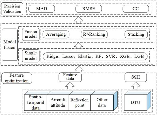
FIGURE 1. Framework of airborne GNSS-R sea surface height retrieval.
Feature Optimization
Feature optimization refers to the process of extracting features from the raw data, which can describe the data better and the performance of the model built with this feature on the unknown data can reach the best (Kim et al., 2019). In numerical data tasks, the importance of feature engineering is particularly prominent. The better the features, the greater the flexibility, and the simpler the model is, the better the performance is. Feature missing or feature redundancy will seriously affect the accuracy of the model. Due to the problems of large feature dimension, high redundancy, strong correlation between adjacent features, the poor correlation between features and the DTU15 model value, in airborne DW data. In this paper the features of airborne DW data are optimized by the methods of feature selection, feature extraction, and feature construction.
1) Feature selection: By eliminating irrelevant or redundant features, the model training time can be reduced, and the accuracy of the model can be improved. The airborne DW data is a set of high-dimensional data. It contains a lot of redundant data and unrelated features for the DTU15 model. Therefore, use the Pearson correlation coefficient method to filter the data set, and the features with correlation coefficient less than 0.1 of DTU15 are removed (Rodgers and Nicewander 1988).
2) Feature extraction: According to the high-dimensional characteristics of airborne data, principal component analysis (PCA) method is used to extract the main feature components of airborne data. PCA is a commonly used data analysis method, which transforms the original data into a group of linear independent representations of each dimension by linear transformation. It can best integrate and simplify the high-dimensional variable system based on retaining the original data information to the maximum extent, and more centrally and typically reflects the characteristics of the research object. The feature values with a cumulative contribution rate of 98% are extracted from the airborne data as training data for machine learning.
3) Feature construction: Feature construction refers to the artificial creation of new feature methods that are beneficial to model training and have certain engineering significance by analyzing raw data samples, combining practical experience of machine learning and professional knowledge in related fields. Therefore, to extract features that contain enough information, three features sensitive to SSH changes, PCP70, PFD, and LES, are constructed on the basis of the raw airborne DW data to improve the accuracy of the altimetry model. The PCP70 and PFD features are calculated from two retracking methods commonly used in GNSS-R SSH retrieval (Park et al., 2013; Clarizia et al., 2016), which can effectively reflect the changes in SSH. Leading Edge Slope (LES) is a feature that has a high correlation with sea surface roughness (Liu et al., 2019). The corresponding definition is as follows:
1) PCP70: This feature has been derived from traditional retracking methods taking the specular reflection delay at 70% of the peak correlation power. The peak correlation power is defined as (Mashburn et al., 2016):
where,
2) PFD This feature also has been derived from traditional retracking methods taking the specular reflection delay from the maximum first derivative on the waveform leading edge. The waveform leading edge peak first derivative is defined as (Mashburn et al., 2016):
3) LES is often used to retrieve the effective wave height changes of ocean surface. Use the best fitted linear function slope as the leading-edge slope of the time-delayed waveform (Liu et al., 2019):
4) Division of feature set: to select features that are sensitive to the sea surface height, a total of six sets of feature sets with different information details are used for model training, and their accuracy is verified on the test set, namely: Feature Set1: Use DW data only. Feature Set2: Use DW data and PCP70 features. Feature Set3: Use DW data and PFD features. Feature Set4: Use DW data and LES features. Feature Set5: Use DW data and PCP70 and PFD features. Feature Set6: Use DW data and PCP70,PFD, LES features.
Model Fusion
Model fusion is mainly divided into three parts: a single model selection and training, model hyperparameter optimization and model fusion. Single model training is mainly used for model screening and hyperparameter optimization. Model fusion refers to the use of different model fusion methods to integrate the advantages of individual learners which can achieve the goal of reducing prediction errors and optimizing overall model performance. Training process uses the five-fold cross-validation method and optimizes hyper-parameters through grid search.
Selection and Training of a Single Model
The SSH retrieval mainly uses the supervised learning regression method in machine learning, and the learners in the regression method can be divided into non-integrated learners and integrated learners. This paper mainly selected Lasso Regression, Ridge Regression, ElasticNet Regression (Zeng 2020), Support Vector Regression (SVR), as the non-integrated learner, and selected Gradient Boosting Decision Tree (GBDT) (Friedman 2001), Extreme Gradient Boosting (XGBoost), Light Gradient Boosting Machine (LightGBM) and Random Forests (RF) ensembled tree model based on bagging integration thoughts (Breiman, 1996) as ensembled learner to retrieve SSH.
Model Hyper-Parameter Optimization
Hyper-parameter optimization is the key to model training. The performance of the trained model mainly depends on the algorithm of the model and the selection of hyper-parameters. A set of optimal hyper-parameters can make the trained model obtain better performance based on the inherent algorithm. In this paper, Grid search (GS) and K-fold cross validation are used to optimize the hyperparameters of each model.
K-Fold Cross Validation (CV) (Zeng 2020) is a method to continuously verify the performance of models. The basic idea is to divide the original data into K groups randomly, and make a validation set for each subset. The rest of K-1 subset as training set. K models will be obtained in this way. The final prediction performance in the validation set is averaged as the performance index of the K-fold cross-validation classifier. In this paper, we choose K = 5 (Jung 2018), that is, we use five-fold cross-validation cross to verify the model.
Grid search (GS) (Lavalle et al., 2004) is an exhaustive search method for tuning parameters. In the selection of all candidate parameters, every possibility is tried through loop traversal. The set of hyper-parameters with the highest model score is the optimal hyper-parameter. The optimization parameters of each model are shown in Table 1 (Zeng 2020):
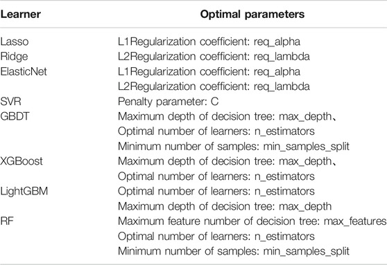
TABLE 1. Summary table of learner optimization parameters.
Model Fusion
Each machine learning algorithm has its own advantages and disadvantages, so it is difficult to fully mine the information in DW data using a single model. Model fusion refers to obtain a new model by combining the results of multiple independent learners. The purpose of model fusion is to break through the limitations of the single machine learning algorithm. Through fusion, the effect of “complementing each other’s weaknesses” can be achieved. Combining the advantages of individual learners can reduce prediction errors and optimize integrated model performance. At the same time, the higher the accuracy and diversity of individual learners, the better the effect of model fusion. This paper uses three model fusion methods: Averaging, R2-Ranking and Stacking for comparative experiments. Averaging and R2-Ranking only merge the results of multiple models, while Stacking needs to use the sub-learner to learn the results of multiple models.
1) Averaging
The output of Average model fusion method is the simple average result of each learner (Liu et al., 2020).
2) R2-Ranking
R2-Ranking is a weighted average model fusion method based on the cross-validation error improvement of the learner on the training set, which is proposed in this paper. The weight is assigned by the coefficient of determination (R2) on the training set. R2 is a commonly used performance evaluation index in machine learning regression models, which reflects the fitting degree of the model to the input data. The closer R2 is to 1, the better the fitting degree is. R2-Ranking believes that under the premise of no fitting, the greater the coefficient of determination of cross-validation on the training set, the better the effect of the learner, so more weight is given. The specific calculation formula is as follows:
Here,
where T is the prediction sequence of the model,
3) Stacking
Stacking is a hierarchical model integration framework. Take two layers as an example: the first layer is composed of multiple base learners whose input is the original training set; the second layer model is trained with the output of the first level basic learner as the training set, so as to obtain a complete Stacking model (Liu et al., 2020). All the training data are used in the two-layer stacking model. This paper uses the stacking model fusion method of five-fold cross-validation, and the construction process is shown in Figure 2:
1) Firstly, the data is divided into training set and test set, and the training set is divided into five parts: train1 ∼5
2) Select the base model: selecting Model1, Model2, and Model3 as the base learners. In Model 1, train1, train2, train3, train4, and train5 are used as the verification set in turn, and the remaining four are used as the training set. Then the model is trained by 5-fold cross-validation, and the prediction is made on the test set. In this way, 5 predictions trained by the XGBoost model on the training set and 1 prediction B1 on the test set will be obtained, and then the 5 predictions will be vertically overlapped and merged to obtain A1. The Model 2 model and the Model 3 model are partially the same.
3) Select the sub-learner: after the training of the three basic models, the predicted values of the three models in the training set are taken as three “features” A1, A2 and A3 respectively, and then use the sub-learner model to train and build the model.
4) Using the trained sub-learner model predict the “feature” values (B1, B2, and B3) obtained on the test sets of the three base models, and the final prediction category or probability is obtained.
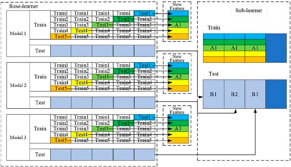
FIGURE 2. Schematic diagram of five fold cross-validation stacking model fusion.
Precision Evaluation
The prediction result is compared with the sea surface height SSH provided by the DTU15 validation model, using Mean Absolute Difference (MAD), Root Mean Square Error (RMSE) and Pearson Correlation Coefficient (CC) (Garrison, 2016) evaluate the effectiveness of the model. It shows: the smaller the MAD and RMSE values are, the better the fitting degree between the predicted value and the real value is, and the smaller the error is; The closer CC is to 1, the better correlation between inversion results and DTU15 model is. The corresponding definition is (Liu et al., 2020; Zeng 2020):
Where T is the prediction sequence of the model, where A is the SSH value verification sequence provided by the corresponding DTU15 model. Here
Verification of New Machine Learning Weighted Average Fusion Feature Extraction Method
Data Sets
Delay Waveform Data
The airborne time delay waveform data which from the airborne experiment was carried out by the IEEC of Spain on December 3, 2015 in the Baltic Sea. As the Baltic Sea is surrounded by land, it is not affected by the strong North sea tide. Under the condition of no strong wind, the sea surface is relatively stable (Wang et al., 2021a). During the experiment, there was no strong wind in the experimental area, and the sea surface was relatively stable. The direct and reflected GNSS signals were received by the 8-element antenna of RHCP (Right Handled Circular Polarization) on the top and LHCP (Left HCP) on the abdomen of the aircraft respectively, and then down converted to IF signal in 19.42 MHz by RF module for 1-bit quantization and storage. The Delay waveform (DW) data was obtained by cross-correlation interference between GPS direct signals and sea surface reflection signals (Serni et al., 2017).
As shown in Figure 3, the flight consisted in a set of passes between two pairs of waypoints (AD and EF). Their location was selected to have two straight flight trajectory intervals: parallel (AD) and perpendicular (EF) to the ellipsoidal height gradient of the sea surface. The flight path consisted in two perpendicular trajectories, which were travelled in both senses (A-to-D, D-to-A, E-to-F, and F-to-E). During all of them, the nominal height of the receiver was around 3 km. Table 2 provides the most relevant information about the different flight segments and the time reference system is GPS second of the day (SoD).
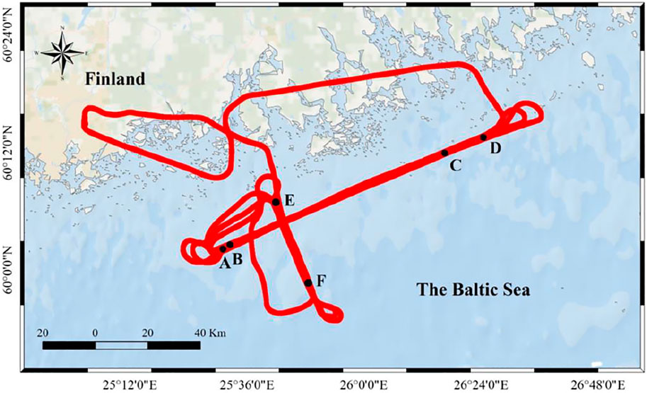
FIGURE 3. Flight trajectory and sea surface height.

TABLE 2. Training results of different models.
In this study, 20 min of GPS L1 band observation data from 10:52:42 to 11:21:41 on December 3, 2015 were used. To avoid the influence of aircraft steering, the data of aircraft steering is removed. Only the data of aircraft flying along a straight line is selected as the experimental analysis. Since the E-F segment is too short to be suitable for machine learning model modeling, this paper uses the D-A segment and B-C segment data as experimental data.
Validation Model
To verify the precision of airborne GNSS-R SSH retrieval, it needs to be compared with the measured sea surface data. Due to the lack of measured data, the verification model is used to verify the precision of SSH retrieval. In this paper, DTU15 (DTU mean sea surface 15) (Mashburn et al., 2018) model developed by Danish University of technology and TPXO8 (Egbert and Erofeeva 2002) global ocean tide model provided by Oregon State University (OSU) are used as the validation model. The sea surface height SSH obtained from the validation model is as follows:
Data Set Matching and Partition
The DW is a continuous time-varying data set, while the DTU15 is a grid data whose longitude and latitude are both 1′. Therefore, it is necessary to match the airborne DW data set with the DTU15 average sea surface model in time and space first, also extract the average sea surface value of DTU15 corresponding to the DW data, and then tide correction for the same time, latitude and longitude of the airborne time-delay waveform was calculated by the TPXO8 global ocean tide model. Finally superimpose it on the DTU15 to get the SSH value of the DTU15 verification model. The airborne delay waveform (DW) data set and the corresponding SSH value constitute the raw data set. Divide the raw data set into three parts: training set, validation set and test set, and use 80% of the second time period (GPST: 385542–386501 s) data as training data for model training; the remaining 20% of the second time period data is used as verification data for the optimization of model hyperparameters and preliminary evaluation of model performance. The experimental data in the first time period (GPST: 384702–385121 s) is used as the test data to evaluate the generalization ability of the model.
Analysis of Height Measurement Accuracy of Different Machine Learning Models
Analysis of Training Results of Different Models
In this paper, a variety of machine learning regression algorithms are used to establish the mapping relationship between the airborne DW data and the DTU15 verification model. The hyperparameters are optimized and the performance of the model is initially evaluated through the R2 of each machine learning model on the verification set. Table 3 shows the training results of each machine learning model after 5-fold cross-validation training. It can be seen that the R2 of the ensembled tree model is significantly higher than that of the non-ensembled learner, and the XGBoost model has the R2 of 0.95, which shows that after XGBoost regression training, and the model can discover the explanatory information that explains 95% of the target factor change from the input factors. But in the non-ensembled learner, the Ridge regression model obtained the highest R2 of 0.78, indicating that after linear regression training, the model can discover the explanatory information that explains 78% of the target factor change from the input factors.
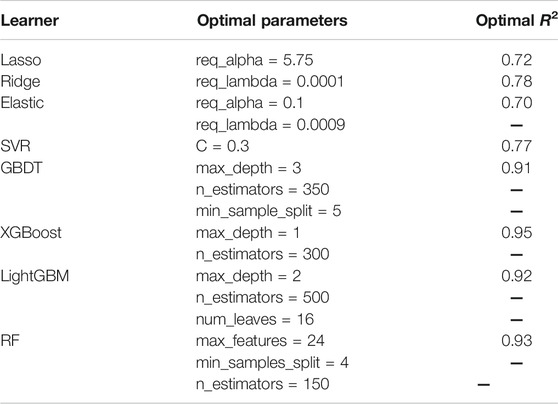
TABLE 3. Training results of different models.
Analysis of Generalization Ability of Different Models
Using the data in the test set to evaluate the generalization ability of the trained model in (1) to verify the final performance of the model. As is shown in Figure 4, the error fitted curve are obtained by making the difference between the results of each machine learning model and the SSH value provided by the DTU15 verification model.
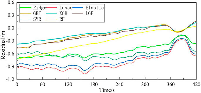
FIGURE 4. Curves chart of forecast errors from different models.
As illustrated in Figure 4 the overall prediction error of the ensembled tree model is relatively small, and the XGB model based on Boosting’s ensembled method has the best prediction results. In the linear regression model, the Ridge model has the best estimate results. At the same time, we can see that retrieval errors of different types of models have great differences. The forecast errors of decision tree models have a significant downward bulge between 360 and 410 s on the time axis, while the linear regression errors have an obvious upward bulge. The data step is mainly due to the loss of a part of the training data (SoD: 40,781–40,842). Because the model with missing training data did not consider the information of the missing data during training, the inversion results of the model on the test set were biased. At the same time, due to the different algorithm rules of the decision tree model and the linear regression model, the two types of models have different emphasis on data information mining, which makes the prediction results different. The data step is mainly caused by the loss of some data in the training data (SOD: 40,781–40,842). Due to the lack of training data, the model does not consider the information of missing data during training, resulting in errors in the inversion results of the model on the test set. At the same time, due to the different algorithm rules of decision tree model and linear regression model, the two types of models have different emphasis on data information mining, resulting in great differences in prediction results.
Height Measurement Accuracy Analysis of Machine Learning Fusion Model
Comparative Analysis of Accuracy Between Single Model and Fusion Model
XGB, RF and ridge models with high accuracy and low correlation are used in the fusion model. Three model fusion methods are compared: Averaging, Stacking and R2-Ranking; among them. Averaging and R2-Ranking only combine the results of multiple models, while Stacking R2-Ranking needs to specify sub-learner. In this paper, the base learner of the Stacking fusion model uses XGB and random forest, and the sub-learner uses Ridge, which has the best retrieval result in the linear model.
Figure 5 illustrates the retrieval results and correlation scatter of XGB, RF and ridge models. Figure 6 illustrates the retrieval results and correlation scatter of Averaging, Stacking and R2-Ranking fusion methods.
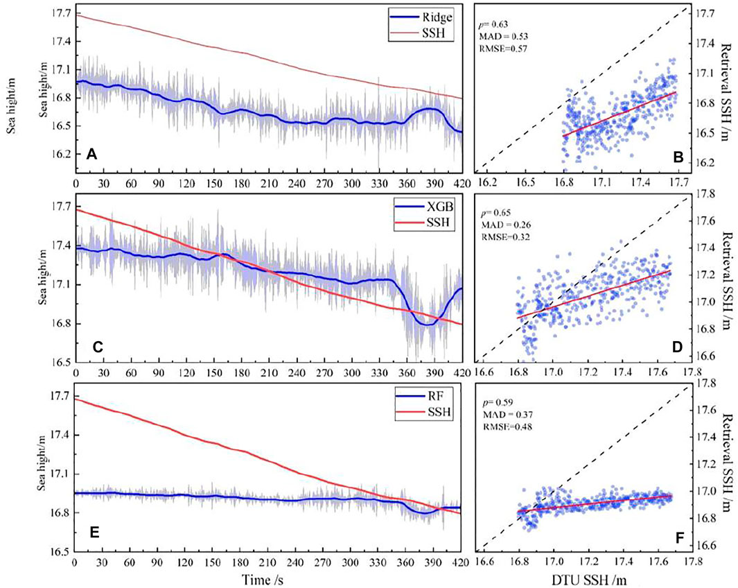
FIGURE 5. Forecast results and correlation scatterers of single model.
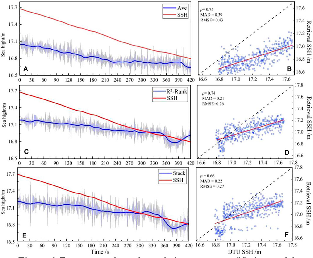
FIGURE 6. Forecast results and correlation scatterers of fusion model.
It can be seen from Figure 5 and Figure 6 that the three fusion models show better predictions compared to single models. The predictions of R2-Ranking and Stacking are closer to the DTU15 model, with smaller errors. The retrieval results of the R2-Ranking and Averaging models have strong correlations with the DTU15 model, which are 0.74 and 0.75, respectively. In summary, in this paper, the R2-Ranking fusion model has the best retrieval performance.
The number of seeds for the 5-fold cross-validation was changed three times and the experiment was repeated to verify the robustness of the fusion model. Changing the number of random seeds is equivalent to re-slicing the original data set and training the base learner again on the new data set. Finally, the performance of the three fusion methods are compared through the retrieval results still on the test set. The performance indices of different models are shown in Table 4. As can be seen from Table 4 that the robustness of the three fusion models is superior. There is no obvious change in the MAD, RMSE, and CC of each model, and the results of the three experiments are basically consistent. The retrieval performance of Averaging, R2-Ranking, and Stacking fusion models is almost better than that of the single model, indicating that fusion model has further improved the model performance.
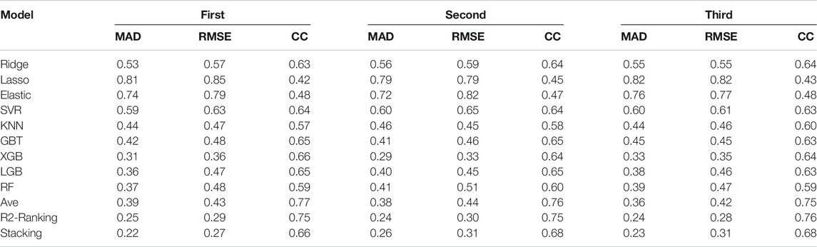
TABLE 4. Comparison of experimental results of different models.
The Impact of Different Features on Model Accuracy
In the field of data mining and machine learning, it is generally believed that the upper limit of machine learning is determined data and features, and the model can only approach the upper limit indefinitely. Therefore, in order to select features that are sensitive to the SSH, a total of six sets of feature sets with varying levels of information details in Feature Optimization are used for model training, and their performance is verified on the test set.
Figure 7A–C present the comparison of the retrieval results (after fitting) of Averaging, R2-Ranking and Stacking fusion models in six different feature sets.
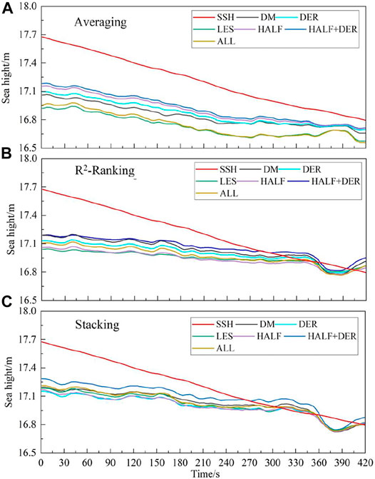
FIGURE 7. Forecast results of three fusion model in different data sets.
It can be seen from Figure 7 that the three fusion models do not achieve the best inversion effect in feature set 6 which contains the most feature information. But the feature set 5, which is composed of DW data, PCP70 and PFD features, shows the best. in other words, the machine learning fusion model with feature set 5 can learn the complex relationship better among the input features, so as to accurately retrieve the SSH.
As the six data sets shown in Table 5 that both the MAD and the RMSE of the feature set 5 are the smallest in all the data sets, that is, the inversion results of the three fusion models on data set 5 are the most accurate. At the same time, the correlation between the retrieval result of data set 5 and the DTU15 model is also the best among the six data sets.

TABLE 5. Comparison of experimental results of different models at different Feature Set.
To compare the inversion accuracy of the three models more Visually on each data set, the polar coordinate system is used to visualize the experimental results, as shown in Figure 8.
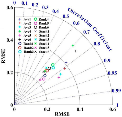
FIGURE 8. Polar chart of prediction performance of fusion mode.
Application of New Machine Learning Weighted Average Fusion Feature Extraction Method
The new GNSS-R SSH retrieval model based on machine learning fusion model and feature optimization used the information of the entire delay waveform for height inversion. The traditional single-point retracking method estimate the time delay by determining the position of the characteristic points of the reflected waveform within the time delay window. The characteristic points of the waveform that have been used for sea surface altimetry include the waveform leading edge peak first derivative (DER) (Mashburn et al., 2016) and the delay of the 70% peak correlation power (HALF) (Mashburn et al., 2016). In order to verify the superiority of the new machine learning weighted average fusion feature extraction method, this paper compared their retrieval performance. The traditional single-point tracking method uses DER and HALF methods to estimate the time-delay of the reflected signal relative to the direct signal. The SSH retrieval algorithms in literature (Mashburn et al., 2016) is used to correct the tropospheric delay and distance error between the antennas. Figure 9 presents the SSH estimates by the HALF, DER retracking method and the new machine learning weighted average fusion feature extraction method. It can be seen from Figure 9 that the retrieval results of the machine learning fusion model are significantly better than the HALF and DER single-point re-tracking methods. Compared with the traditional retracking method, the prediction result of the R2-Ranking fusion model is more stable and closer to the SSH value. Moreover, the machine learning fusion model does not need to consider various error corrections in the time-delay retrieval algorithms, which partly simplifies the complexity of retrieval model.
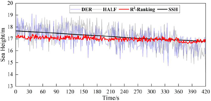
FIGURE 9. Forecast results of R2 ranking fusion model and single point retracking method.
Table 6 presents the precision index of the three models, which shows that the machine learning fusion model is obviously superior to the retracking method of HALF and DER on MAD, RMSE and CC. The application of the new machine learning weighted average fusion feature extraction method effectively improves the accuracy of SSH retrieval, in which the mean absolute error (MAD) is reduced by 63.1 and 59.2% respectively, and the root mean square error (RMSE) is reduced by 63.3 and 61.8% respectively; The correlation coefficient (CC) increased by 31.6 and 44.2% respectively.

TABLE 6. Comparison of SSH retrieval performance between R2-Ranking fusion model and single point retracking methods.
Conclusion and Prospect
The traditional single-point retracking method is an empirical model, which can only use a small amount of DDM information. This method will cause information waste and loss of certain inversion accuracy. In order to improve the accuracy of SSH retrieval, this paper proposed a new type of machine learning weighted average fusion feature extraction method and analyze the inversion accuracy of different models and the influence of different feature sets on the model. The specific conclusion are as follows:
1) This paper first evaluates the SSH retrieval performance of regression methods commonly used in machine learning, such as linear regression model (Lasso, Ridge) SVR and ensembled tree regression model (XGBoost, LightGBM and RF). The experimental results show that the ensembled tree regression model have an overall outstanding performance on the test set, and the effects of other models are slightly worse.
2) RF, XGBoost and Ridge models with better SSH retrieval performance and lower correlation are used for model fusion, which further improves the SSH retrieval accuracy. Three model fusion methods: Averaging, R2-Ranking and Stacking are used for model fusion. The experimental results show that the retrieval accuracy and correlation of the SSH value fusion model compared with the DTU15 validation model are better than a single model, and the fusion further improves the effect of the model. At the same time, the R2-Ranking fusion method proposed in this paper achieved the most accurate retrieval results, with a mean absolute error of about 0.25, a root mean square error RMSE of about 0.29, and a correlation CC of about 0.75.
3) In order to obtain a better feature set, feature engineering methods are used to screen and construct features that are highly sensitive to the sea surface. This paper uses a total of six groups of feature sets with different information details for model training and verifies its accuracy on the test set. Experimental results show that the three fusion models have the best retrieval accuracy on feature set 5 that includes DW, PCP70 and PFD features. It shows that the machine learning fusion model with feature set of 5 can better learn the complex relationship between the original input features, so as to accurately retrieve the height.
4) By comparing the retrieval results with the commonly used DER and HALF traditional single-point tracking methods, it is concluded that the new machine learning weighted average fusion feature extraction method effectively improves the precision of SSH retrieval. The precision has been improved by 61, 61, and 44% respectively in MAD, RMSE and CC.
The new machine learning weighted average fusion feature extraction method proposed in this paper provides a new idea for the future DDM-based GNSS-R sea surface altimetry verification star height inversion. The method proposed in this paper can be extended to a wider scientific fields, such as: GNSS-R sea surface wind speed retrieval, sea ice and soil moisture detection, etc. Only need to re-optimize the features and modify the input and corresponding output data. Compared with the previous inversion models, machine learning algorithms are easier to build models, without the need to build multiple error models, and can make full use of the physical quantities related to the sea surface height, and have a good accuracy. The disadvantage is that the machine learning model requires a large number of labeled observations to train and build the model. The spaceborne GNSS-R receiver can provide massive observation data. However, the corresponding high-precision sea surface height is difficult to obtain. Meanwhile, since the GNSS-R signal is weak, how to construct features sensitive to SSH change is another main factor of SSH inversion by machine learning fusion model. In the next step, more physical parameters related to sea surface height can be extracted to improve the effect of the fusion model.
Data Availability Statement
The original contributions presented in the study are included in the article/Supplementary Material, further inquiries can be directed to the corresponding authors.
Author Contributions
QW: scientific analysis and manuscript writing. WZ and FW: experiment design, project management, review and editing. QW, WZ, and FW contributed equally to this paper. All authors contributed to the article and approved the submitted version.
Funding
This work was supported by the National Natural Science Foundation of China under Grant (41774014, 41574014), the Liaoning Revitalization Talents Program under Grant (XLYC2002082), the Frontier Science and Technology Innovation Project and the Innovation Workstation Project of Science and Technology Commission of the Central Military Commission under Grant (085015), the Independent Research and Development Start-up Fund of Qian Xuesen Laboratory of Space Technology (Y-KC-WY-99-ZY-000-025), and the Outstanding Youth Fund of China Academy of Space Technology.
Conflict of Interest
The authors declare that the research was conducted in the absence of any commercial or financial relationships that could be construed as a potential conflict of interest.
Publisher’s Note
All claims expressed in this article are solely those of the authors and do not necessarily represent those of their affiliated organizations, or those of the publisher, the editors and the reviewers. Any product that may be evaluated in this article, or claim that may be made by its manufacturer, is not guaranteed or endorsed by the publisher.
Acknowledgments
We would like to thank Institute of Space Sciences (ICE, CSIC) and Institute for Space Studies of Catalonia (IEEC) for providing the raw data processing results of the air-borne experiment.
References
Alonso-Arroyo, A., Zavorotny, V. U., and Camps, A. (2017). Sea Ice Detection Using U.K. TDS-1 GNSS-R Data. IEEE Trans. Geosci. Remote Sensing. 55, 4989–5001. doi:10.1109/TGRS.2017.2699122
Bai, W., Xia, J., Wan, W., Zhao, L., Sun, Y., Meng, X., et al. (2015). A First Comprehensive Evaluation of China's GNSS-R Airborne Campaign: Part II-River Remote Sensing. Sci. Bull. 60, 1527–1534. doi:10.1007/s11434-015-0869-x
Bosch, W., Dettmering, D., and Schwatke, C. (2014). Multi-Mission Cross-Calibration of Satellite Altimeters: Constructing a Long-Term Data Record for Global and Regional Sea Level Change Studies. Remote Sensing. 6, 2255–2281. doi:10.3390/rs6032255
Cardellach, E., Rius, A., Martín-Neira., M., Fabra, F., Nogues-Correig, O., Ribo, S., et al. (2014). Consolidating the Precision of Interferometric GNSS-R Ocean Altimetry Using Airborne Experimental Data. IEEE Trans. Geosci. Remote Sensing. 52, 4992–5004. doi:10.1109/TGRS.2013.2286257
Clarizia, M. P., Ruf, C., Cipollini, P., and Zuffada, C. (2016). First Spaceborne Observation of Sea Surface Height Using GPS‐Reflectometry. Geophys. Res. Lett. 43, 767–774. doi:10.1002/2015GL066624
D'Addio, S., Martín-Neira, M., di Bisceglie, M., Galdi, C., and Martin Alemany, F. (2014). GNSS-R Altimeter Based on Doppler Multi-Looking. IEEE J. Sel. Top. Appl. Earth Observations Remote Sensing. 7, 1452–1460. doi:10.1109/JSTARS.2014.2309352
Egbert, G. D., and Erofeeva, S. Y. (2002). Efficient Inverse Modeling of Barotropic Ocean Tides. J. Atmos. Oceanic Technol. 19, 183–204. doi:10.1175/15200426(2002)0192.0.CO10.1175/1520-0426(2002)019<0183:eimobo>2.0.co;2
Friedman, H. (2001). Greedy Function Approximation: a Gradient Boosting Machine. Ann. Stat. 29, 1189–1232. doi:10.2307/269998610.1214/aos/1013203451
Garrison, J. L. (2016). A Statistical Model and Simulator for Ocean-Reflected GNSS Signals. IEEE Trans. Geosci. Remote Sensing. 54, 6007–6019. doi:10.1109/TGRS.2016.2579504
Hoerl, A. E., and Kennard, R. W. (1970). Ridge Regression: Biased Estimation for Nonorthogonal Problems. Technometrics. 12, 55–67. doi:10.1080/00401706.1970.10488634
Jia, Y., Jin, S., Savi, P., Gao, Y., Tang, J., Chen, Y., et al. (2019). GNSS-R Soil Moisture Retrieval Based on a XGboost Machine Learning Aided Method: Performance and Validation. Remote Sensing. 11, 1655–1779. doi:10.3390/rs11141655
Jing, C., Niu, X., Duan, C., Lu, F., Di, G., and Yang, X. (2019). Sea Surface Wind Speed Retrieval From the First Chinese GNSS-R Mission: Technique and Preliminary Results. Remote Sensing. 11, 3013–3025. doi:10.3390/rs1112143810.3390/rs11243013
Jung, Y. (2018). Multiple PredictingK-Fold Cross-Validation for Model Selection. J. Nonparametric Stat. 30, 197–215. doi:10.1080/10485252.2017.1404598
Keerthi, S. S., Shevade, S. K., Bhattacharyya, C., and Murthy, K. R. K. (2001). Improvements to Platt's SMO Algorithm for SVM Classifier Design. Neural Comput. 13, 637–649. doi:10.1162/089976601300014493
Kim, H., Lee, S., Lee, S., Hong, S., Kang, H., and Kim, N. (2019). Depression Prediction by Using Ecological Momentary Assessment, Actiwatch Data, and Machine Learning: Observational Study on Older Adults Living Alone. JMIR Mhealth Uhealth. 7, e14149–14149. doi:10.2196/14149
Lary, D. J., Alavi, A. H., Gandomi, A. H., and Walker, A. L. (2016). Machine Learning in Geosciences and Remote Sensing. Geosci. Front. 7, 3–10. doi:10.1016/j.gsf.2015.07.003
Lavalle, S. M., Branicky, M. S., and Lindemann, S. R. (2004). On the Relationship Between Classical Grid Search and Probabilistic Roadmaps. Int. J. Robotics Res. 23, 673–692. doi:10.1007/978-3-540-45058-0_510.1177/0278364904045481
Li, W., Cardellach, E., Fabra, F., Rius, A., Ribó, S., and Martín-Neira, M. (2017). First Spaceborne Phase Altimetry over Sea Ice Using TechDemoSat-1 GNSS-R Signals. Geophys. Res. Lett. 44, 8369–8376. doi:10.1002/2017GL074513
Li, X., Yang, D., Yang, J., Zheng, G., Han, G., Nan, Y., et al. (2021). Analysis of Coastal Wind Speed Retrieval From CYGNSS mission Using Artificial Neural Network. Remote Sensing Environ. 260, 112454–112466. doi:10.1016/j.rse.2021.112454
Liu, L., Sun, Y., Bai, W., and Luo, L. (2020). The Inversion of Sea Surface Wind Speed in GNSS-R Base on the Model Fusion of Data Mining. Geomatics Inf. Sci. Wuhan Univ. 12, 1–10. doi:10.13203/j.whugis2019038310.3390/rs12122034
Liu, Y., Collett, I., and Morton, Y. J. (2019). Application of Neural Network to GNSS-R Wind Speed Retrieval. IEEE Trans. Geosci. Remote Sensing. 57, 9756–9766. doi:10.1109/tgrs.2019.2929002
Luo, L., Bai, W., Sun, Y., and Xia, J. (2020). GNSS-R Sea Surface Wind Speed Inversion Based on Tree Model Machine Learning Method. China. J. Space Sci. 40, 595–601. doi:10.11728/cjss2020.04.595
Martin-Neira, M. (1993). A Passive Reflectometry and Interferometry System (PARIS): Application to Ocean Altimetry. ESA J. 17, 331–355.
Mashburn, J., Axelrad, P., Lowe, S. T., and Larson, K. M. (2018). Global Ocean Altimetry with GNSS Reflections From TechDemoSat-1. IEEE Trans. Geosci. Remote Sensing. 56, 4088–4097. doi:10.1109/TGRS.2018.2823316
Mashburn, J., Axelrad, P., T. Lowe, S. S., and Larson, K. M. (2016). An Assessment of the Precision and Accuracy of Altimetry Retrievals for a Monterey bay GNSS-R Experiment. IEEE J. Sel. Top. Appl. Earth Observations Remote Sensing. 9, 4660–4668. doi:10.1109/jstars.2016.2537698
Mashburn, J., Axelrad, P., Zuffada, C., Loria, E., O'Brien, A., and Haines, B. (2020). Improved GNSS-R Ocean Surface Altimetry With CYGNSS in the Seas of indonesia. IEEE Trans. Geosci. Remote Sensing. 58, 6071–6087. doi:10.1109/tgrs.2020.2973079
Park, H., Valencia, E., Camps, A., Rius, A., Ribo, S., and Martin-Neira, M. (2013). Delay Tracking in Spaceborne GNSS-R Ocean Altimetry. IEEE Geosci. Remote Sensing Lett. 10, 57–61. doi:10.1109/LGRS.2012.2192255
Ribó, S., Arco-Fernández, J., Cardellach, E., Fabra, F., Li, W., Nogués-Correig, O., et al. (2017). A Software-Defined GNSS Reflectometry Recording Receiver With Wide-Bandwidth, Multi-Band Capability and Digital Beam-Forming. Remote Sensing. 9, 450. doi:10.3390/rs9050450
Rodgers, J. L., and Nicewander, W. A. (1988). Thirteen Ways to Look at the Correlation Coefficient. The Am. Statistician. 42, 59–66. doi:10.2307/2685263
Ruf, C. S., Atlas, R., Chang, P. S., Clarizia, M. P., Garrison, J. L., Gleason, S., et al. (2016). New Ocean Winds Satellite Mission to Probe Hurricanes and Tropical Convection. Bull. Am. Meteorol. Soc. 97, 385–395. doi:10.1175/BAMS-D-14-00218.1
Wang, F., Yang, D., Zhang, G., and Zhang, B. (2021a). Measurement of Sea Surface Height Using Airborne Global Navigation Satellites System Reflectometry. Acta Aeronautica et Astronautica Sinica. 42, 324852. doi:10.7527/S1000-6893.2020.24852
Wang, J., Xu, H., Yang, L., Song, Q., and Ma, C. (2021b). Cross-Calibrations of the HY-2B Altimeter Using Jason-3 Satellite During the Period of April 2019-September 2020. Front. Earth Sci. 9, 215–231. doi:10.3389/feart.2021.647583
Xu, L., Wan, W., Chen, X., Zhu, S., Liu, B., and Hong, Y. (2019). Spaceborne GNSS-R Observation of Global lake Level: First Results from the TechDemoSat-1 Mission. Remote Sensing. 11, 1438–1448. doi:10.3390/rs11121438
Yan, S., Zhang, N., Chen, N., and Gong, J. (2019). Using Reflected Signal Power From the BeiDou Geostationary Satellites to Estimate Soil Moisture. Remote Sensing Lett. 10, 1–10. doi:10.1080/2150704X.2018.1519272
Zawadzki, L., and Ablain, M. (2016). Accuracy of the Mean Sea Level Continuous Record With Future Altimetric Missions: Jason-3 vs. Sentinel-3a. Ocean Sci. 12, 9–18. doi:10.5194/osd-12-1511-201510.5194/os-12-9-2016
Zeng, Z. (2020). A Study on Alpha Strategy's Quantitative Investment (In Chinese). Guangzhou: Jinan University.
Zhang, Y., Zhang, Y., Meng, T., and Yang, H. (2020). Research on Sea Surface Altimetry Model of Airborne GNSS Reflected Signal. Acta Oceanologica Sinica. 42, 149–156. doi:10.3969/j.issn
Keywords: GNSS-r altimetry, machine learning, wave retracking, sea surface height inversion, feature engineering, model fusion
Citation: Wang Q, Zheng W, Wu F, Xu A, Zhu H and Liu Z (2021) A New GNSS-R Altimetry Algorithm Based on Machine Learning Fusion Model and Feature Optimization to Improve the Precision of Sea Surface Height Retrieval. Front. Earth Sci. 9:730565. doi: 10.3389/feart.2021.730565
Received: 25 June 2021; Accepted: 16 August 2021;
Published: 27 August 2021.
Edited by:
Jinyun Guo, Shandong University of Science and Technology, ChinaReviewed by:
Yongchao Zhu, Hefei University of Technology, ChinaKonstantinos Demertzis, International Hellenic University, Greece
Copyright © 2021 Wang, Zheng, Wu, Xu, Zhu and Liu. This is an open-access article distributed under the terms of the Creative Commons Attribution License (CC BY). The use, distribution or reproduction in other forums is permitted, provided the original author(s) and the copyright owner(s) are credited and that the original publication in this journal is cited, in accordance with accepted academic practice. No use, distribution or reproduction is permitted which does not comply with these terms.
*Correspondence: Wei Zheng, emhlbmd3ZWkxQHF4c2xhYi5jbg==; Fan Wu, d3VmYW5AcXhzbGFiLmNu
†These authors have contributed equally to this work