Variations of the seismic b-value along the Dead Sea transform

Sharon, Matty; Kurzon, Ittai; Wetzler, Nadav; Sagy, Amir; Marco, Shmuel; Ben-Avraham, Zvi

doi:10.3389/feart.2022.1074729

ORIGINAL RESEARCH article

Front. Earth Sci., 21 December 2022

Sec. Structural Geology and Tectonics

Volume 10 - 2022 | https://doi.org/10.3389/feart.2022.1074729

This article is part of the Research Topic Tectonic Faults: Types, Characteristics and Behavior View all 7 articles

Variations of the seismic b-value along the Dead Sea transform

Matty Sharon^1,2,3

¹Geological Survey of Israel, Jerusalem, Israel
²Department of Geophysics, Tel Aviv University, Tel Aviv, Israel
³Institute of Earth Sciences, Hebrew University of Jerusalem, Jerusalem, Israel

The frequency-magnitude distribution follows the Gutenberg-Richter empirical law, in which the scaling between small and large earthquakes is represented by the b-value. Laboratory experiments have shown that the b-value is related to fault mechanics with an inverse dependency to the differential stress, as was also inferred from observational datasets through relations with earthquake depth and style of faulting. In this study, we aim to obtain a better understanding of the geological structure and tectonics along the Dead Sea transform (DST), by examining relations of the b-value to three source parameters: the earthquake depth, the seismic moment release, and the predominant style of faulting. We analyse a regional earthquake catalogue of ∼20,300 earthquakes that were recorded between 1983 and 2020 in a regional rectangle between latitudes 27.5°N−35.5°N and longitudes 32°E−38°E. We convert the duration magnitudes, Md, to moment magnitudes, Mw, applying a new regional empirical relation, by that achieving a consistent magnitude type for the entire catalogue. Exploring the variations in the b-value for several regions along and near the DST, we find that the b-value increases from 0.93 to 1.19 as the dominant style of faulting changes from almost pure strike-slip, along the DST, to normal faulting at the Galilee, northern Israel. Focusing on the DST, our temporal analysis shows an inverse correlation between the b-value and the seismic moment release, whereas the spatial variations are more complex, showing combined dependencies on seismogenic depth and seismic moment release. We also identify seismic gaps that might be related to locking or creeping of sections along the DST and should be considered for hazard assessment. Furthermore, we observe a northward decreasing trend of the b-value along the DST, which we associate to an increase of the differential stress due to structural variations, from more extensional deformation in the south to more compressional deformation in the north.

1 Introduction

One of the most fundamental observations in earthquake seismology is that the frequency-magnitude relation follows the Gutenberg-Richter empirical law (Gutenberg and Richter, 1944):

\log [N] = a - b M (1)

where N is the cumulative number of earthquakes of at least a magnitude M; and a and b are seismicity parameters.

Whilst the a-value reflects the seismic activity level and unless normalised, varies in different time windows, the b-value reflects the proportion between small and large earthquakes, and thus has a significant impact for hazard evaluations (Frankel, 1995; Petersen et al., 2011; Marzocchi and Taroni, 2014; Magrin et al., 2017; Sokolov et al., 2017). Yet, some observations suggest that the frequency-magnitude relation (Eq. 1) might deviate at the upper bound of the magnitude distribution, since some fault zones are characterised with repeated large earthquakes of approximately the same size (i.e., “characteristic” behaviour; Wesnousky et al., 1983; Schwartz and Coppersmith, 1984).

Although a b-value of a unity has been previously suggested on a global scale based on real-data analyses (Frohlich and Davis, 1993; Felzer et al., 2004; El-Isa and Eaton, 2014) and theoretical considerations (King, 1983), other studies have been aimed to understand its variations with regards to earthquake mechanics (e.g. Scholz, 1968, 2015; Main et al., 1989; Henderson and Main, 1992; Lei et al., 2000; Tan et al., 2019). It has been previously demonstrated that the b-value varies with the style of faulting, with typical values of 0.7–0.8, 0.9–1.0, and 1.1–1.2 for thrust, strike-slip and normal faulting, respectively, with values in-between for oblique faulting (Schorlemmer et al., 2005; Petruccelli et al., 2019a). This dependency has been shown by other studies as well (Gulia and Wiemer, 2010; Scholz, 2015; Bora et al., 2018; Beall et al., 2022), suggesting an inverse correlation of the b-value with the differential stress, considering the Anderson theory of faulting (Anderson, 1905). The inverse dependency of the b-value with the differential stress has been also shown through rock fracture experiments (Scholz, 1968; Amitrano, 2003; Rivière et al., 2018), and dependency with the earthquake depth considering rheological models (Mori and Abercrombie, 1997; Gerstenberger et al., 2001; Spada et al., 2013; Scholz, 2015; Rigo et al., 2018). In such cases, the b-value has been observed to decrease with depth, within the brittle part of the earth’s crust.

Previous estimations of the frequency-magnitude relation in the region of Israel (Ben-Menahem, 1981, 1991; Salamon et al., 1996; Shapira and Hofstetter, 2002; Hamiel et al., 2009) were mainly focused on hazard perspective, and had limited data for investigating variations of the b-value. In this study we systematically calculate the b-value, focusing on ∼500-km of the southern part of the Dead Sea transform (DST), a ∼1,000-km long continental transform plate boundary that links between the Red Sea spreading centre and the convergence zone in southern Turkey (e.g., Garfunkel, 2014). Our purpose is to investigate variations of the b-value and their relation to the earthquake depth, the style of faulting, and the seismic moment release; hence examining whether and to what extent does the b-value relate to mechanical properties of the fault zone. We examine spatial variations of the b-value with the seismogenic depth, which we estimate according to the 75th and 95th percentiles of the seismicity depth distribution, because they reflect the alteration in the seismogenic depth along the DST (e.g., Shalev et al., 2013; Wetzler and Kurzon, 2016). Possible correlations with the seismic moment release are examined in both space (e.g., Bora et al., 2018) and time (e.g. Cao and Gao, 2002) analyses, for receiving insights about the seismicity of the region and for further understanding variations of the b-value.

Determination of the b-value is often limited within spatial zones, based on seismological or tectonic considerations, which in many cases reflect the dominant style of faulting (e.g. Radulian et al., 2000, 2018; Bala et al., 2003; Bus et al., 2009) and may also be implemented for hazard evaluation purposes (Frankel, 1995; Helmstetter et al., 2006; Yadav et al., 2012; Ashish et al., 2016; Maiti and Kamai, 2020; Mandal et al., 2021; Yagoda-Biran et al., 2021). A preliminary seismogneic zonation in the region (Shamir et al., 2001) and its following analysis of the frequency-magnitude relation (Shapira and Hofstetter, 2002) were based on a rather sparse seismological dataset. A more recent seismogenic zonation (Sharon, 2020) was based on the density distribution of epicentres and seismic moment release, and their spatial relation to the main seismic sources (Sharon et al., 2020). However, this zonation is not adequate to show systematic relation between the b-value and the faulting style because many of these previous zones are too small to achieve well-determined b-value with our current data. For this purpose, we introduce here a rather simplified and broad new tectonic zonation in the DST and its periphery, according to the seismic network capability and the local tectonics.

In this study we first relocate the earthquakes recorded between January 1983 and September 2020 (Wetzler and Kurzon, 2016). Then, due to inconsistent magnitude type within the original catalogue, we generated a catalogue, choosing M_w as the preferred homogenous magnitude type, since it is physical-based and is not saturated at high magnitudes (Kanamori, 1977; Hanks and Kanamori, 1979). Subsequently, we estimate the completeness magnitude, $M_{c}$ , and calculate the frequency-magnitude parameters with respect to the seismogenic depth, the seismic moment release and the tectonic regime associated with the prevailing style of faulting. Specifically, we perform a systematic and thorough spatio-temporal investigation of the b-value at the DST and its periphery.

2 Tectonic settings

The DST was formed during the Miocene, as the African-Arabian plate broke, generating the Suez rift and the DST. While the Suez rift has shown minor signs of post-Miocene deformation, the DST is considered to be the main source of post-Miocene deformation in the region (Garfunkel and Bartov, 1977; Joffe and Garfunkel, 1987; Steckler et al., 1988). It consists of a ∼1000-km long ∼N-S orientated fault system, which is the largest in the Levant (Figure 1). Evaluation from geologic and geodetic sources indicate Quaternary slip rates of 4–5 mm/yr (Garfunkel, 2010; Sadeh et al., 2012; Marco and Klinger, 2014; Hamiel et al., 2018). Our study focuses on the southern section of the DST (Figure 1), dominated by a left-lateral strike-slip overall displacement of ∼105-km accumulated over the past ∼16–20 million years (Quennell, 1959; Garfunkel, 1981, 2014; Nuriel et al., 2017).

FIGURE 1

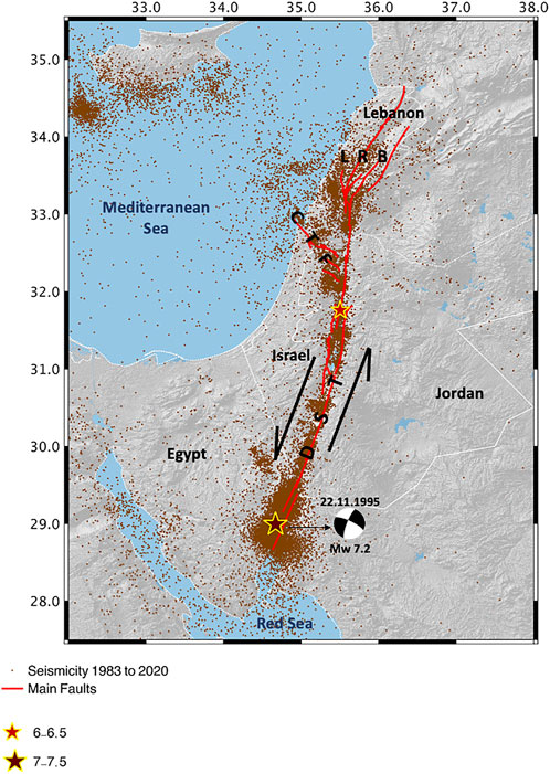
FIGURE 1. Seismic map of the study area showing the main fault segments of the Dead Sea transform (DST) and of the northwest orientated Carmel-Tirza fault system (CTF) system (Sharon et al., 2020); recorded seismicity of 1983–2020 (expansion of Wetzler and Kurzon 2016 catalogue), highlighting the most significant events in the past century: the 1927 M six at the northern Dead Sea, and the M_W 7.2 at the Gulf of Elat (Aqaba). Black arrows denote the relative plate motion along the DST.

The lateral motion on the DST occurs on left-stepping strike-slip and oblique-slip fault segments that delimit a string of en-echelon arranged pull-apart basins (Garfunkel, 1981; Zak and Freund, 1981; Garfunkel and Ben-Avraham, 2001). The DST is topographically expressed by a pronounced 5–25 km wide valley, bordered by normal faults that extend along the valley margins. The north-eastern edge of the study area comprises the Lebanon restraining bend (LRB; Figure 1), where the DST is branched into several segments, transferring the strike-slip motion into the Lebanon area (Gomez et al., 2003, 2007). The northern section of the DST crosses northwest Syria in a N-S orientation, most of it outside our study area.

South of Lebanon, the Sinai sub-plate has several fault systems, associated with Quaternary internal-deformation: the Carmel-Tirza fault zone (CTF; Figure 1) divides the Israel-Sinai sub-plate into two tectonic domains (Neev et al., 1976; Ben-Avraham and Ginzburg, 1990; Sadeh et al., 2012) where the southern part is more rigid, while the northern consists of a set of graben-and-horst structures with E-W-striking normal faults associated with S-N extension (Ron and Eyal, 1985). The CTF consists of SE-NW orientated fault segments, with normal and oblique motions (Freund, 1970). It is associated with coeval motion of ∼0.7 mm/yr left-lateral slip and ∼0.6 mm/yr extension rates (Sadeh et al., 2012), with recent seismicity in its eastern side that sprawl over several parallel fault segments (Hofstetter et al., 1996; Sharon et al., 2020).

To the south of the CTF, several ∼E-W striking faults are associated with mainly dextral slip and some normal faulting (Bentor and Vroman, 1954; Bartov, 1974; Zilberman et al., 1996), which occurred mainly during the Neogene or in earlier periods (Weinberger et al., 2020). An additional fault system of ∼NNE striking faults in southern Israel is associated with normal faulting and minor extension component along the transform system, and was more active during Quaternary times (Bartov et al., 1998; Avni et al., 2000, 2001; Calvo and Bartov, 2001; Marco, 2007).

The potential for strong earthquakes along the DST is demonstrated by the earthquakes of the 1927 M_L 6.2 near Jericho, north of the Dead Sea (Shapira et al., 1993), and the 1995 M_W 7.2 Nuweiba (Hofstetter et al., 2003) in the Gulf of Elat (Aqaba), along with pre-instrumental records, leading to estimations of up to M_W ∼7.5 (Ambraseys, 2009; Agnon, 2014; Marco and Klinger, 2014; Zohar et al., 2016, 2017; Lu et al., 2020). Deep-crust seismicity, correlated with low heat flow areas, particularly in the Dead Sea basin, probably indicates a cold crust, with deep brittle to ductile transition zone (Aldersons et al., 2003; Shalev et al., 2007, 2013; Aldersons and Ben-Avraham, 2014; Wetzler and Kurzon, 2016).

3 Seismological dataset

We analyse an earthquake catalogue from 1 January 1983 until 28 September 2020, recorded by ∼210 stations. The majority of the data originates in the stations of the Israel Seismic Network (ISN), including many new stations deployed under the framework of the TRUAA network, established for the purpose of Earthquake Early Warning System for the state of Israel (Kurzon et al., 2020). In addition, some of the data comes from local CTBT and CNF stations (Comprehensive Nuclear Test-Ban Treaty, and Cooperating National Facility, respectively), and a minority originates in stations of other networks: the GEOFON global network of GFZ, the JSO seismic observatory of Jordan and the CQ seismic network of Cyprus.

In the original catalogue, documented by the ISN, there are 23,316 earthquakes between the latitudes $27.5 ° - 35.5 ° N$ and longitudes $32 ° - 38 ° E$ , referred here as the Rectangular Area (RA; Figure 1). Following Wetzler and Kurzon (2016), we applied similar procedure and methods for earthquake relocation: applying the regional velocity model of Gitterman et al. (2005), earthquakes are located by the genloc library (Pavlis et al., 2004) of the Antelope seismic software package (<www.brtt.com>). Horizontal median errors are 420 m in longitude, 510 m in latitude, and the vertical median error is 750 m, calculated according to Pavlis (1986). The relocated catalogue has ∼23,200 events (Figure 1), with improved locations, and loosing less than 0.5% of the events due to large location errors. The magnitude range of the catalogue is $0.1 \leq M \leq 7.2$ , from which ∼2,900 are with unknown magnitudes (Table 1).

TABLE 1

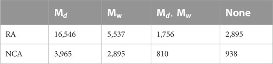
TABLE 1. The number of $M_{d}$ and $M_{w}$ magnitudes, determined for the investigated catalogue. The right-most field is for events that contain no magnitude.

The catalogue includes two magnitude types: duration magnitude (M_d) and the moment magnitude (M_w). Table 1 summarises the two types of magnitude that were determined for the relocated catalogue. The magnitudes of the M_w 7.2 1995 Nuweiba earthquake and the M_w 5.1 2004 Dead Sea earthquake were fixed according to Hofstetter et al. (2003) and Hofstetter et al. (2008), respectively.

The detection sensitivity of the seismic network is primarily dependent on the background noise and the distribution of seismic stations. The seismic network coverage area (NCA; Figure 2) was recently determined by Sharon et al. 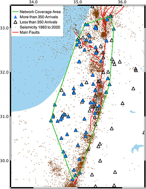(2020) according to the total threshold number of wave arrivals at seismic stations, accounting for their spatial distribution, hence, including hypocentres that are relatively well-constrained, with relatively low magnitude of completeness ( $M_{c})$ . Therefore, determination of the frequency-magnitude parameters within the NCA can be based on more data, consisting of a larger range of magnitudes.

FIGURE 2

FIGURE 2. Seismic stations utilised for recording the earthquakes of the examined catalogue, and the ensuing seismic network coverage area (NCA) delimited by the green polygon.

4 The frequency-magnitude relation

4.1 Magnitude conversion

Earthquake magnitude can be estimated by a wide range of methods and parameters, depending on the spectral properties of the source, the seismic phases, the instrumentation capabilities, and the consideration of path and site effects. Therefore, magnitude estimation does not behave uniformly for all magnitude ranges, and also saturates at different levels (Kanamori, 1977, 1983; Utsu, 2002). Thus, magnitude conversion to a single type of magnitude is vital for seismological analyses that require homogenous earthquake catalogue with consistent magnitude type, such as analysis of the frequency-magnitude relation.

The moment magnitude (M_w) is based on the physical dimensions of the seismic source, does not saturate at extreme rupture size, and hence is more adequate to represent a wide range of magnitudes (Kanamori, 1977; Hanks and Kanamori, 1979; Choy and Boatwright, 1995). Therefore, a common practice is converting other magnitude types to M_w (Scordilis, 2006; Yadav et al., 2009, 2012; Ross et al., 2016; Kumar et al., 2020), which is widely used as a unified magnitude for seismological and hazard-related applications (e.g. Bormann and Di Giacomo, 2011). In the original Israel catalogue, about 70% of the events are assigned only with M_d, without M_w, and less than 10% are estimated by both magnitude types. Therefore, by converting M_d to M_w, we intent to achieve a catalogue of a uniform magnitude type, M_w, that can be the basis for the current seismological analysis, as well as for future investigations.

Considering that many of the magnitude types are determined by a set of parameters, varying according to geological, seismological and instrumentational settings, there is no global formula that converts between $M_{d}$ and $M_{w}$ ; hence, unique formulas are deduced for different regions. A few regression techniques have been suggested and employed for converting magnitudes, and the justification for applying a single method or the other, are based either on theory or empirical observations (e.g. Yadav et al., 2012; Kadirioğlu and Kartal, 2016; Das et al., 2018). In this study we examine M_d to M_w conversion, applying both, ordinary least squares (OLS) regressions, (e.g. Scordilis, 2006; Castello et al., 2007; Ataeva et al., 2015; Ross et al., 2016), and orthogonal regression (OR; e.g., Glaister, 2005; Castellaro et al., 2006; Kane and Mroch, 2020).

Although it is more common to convert magnitudes through linear regressions, Ataeva et al. (2015) added a quadratic regression and obtained better fit to observations in the same region. We examine their approach for M_d to M_w conversion, fitting both linear and quadratic regressions. For comparison, we also examine part of their obtained regressions on the much larger data utilised here.

The regression coefficients published by Ataeva et al. (2015) were deduced in the forms of:

\log [M_{0}] = a * M_{d} + b (2)

and

\log [M_{0}] = a * M_{d}^{2} + b * M_{d} + c (3)

for the linear and quadratic regressions, respectively. We convert M₀ to M_w following the relationship (Hanks and Kanamori, 1979; Aki and Richards, 2002):

M w = \frac{2}{3} [\log [M_{0}] - 9.1] (4)

referring to $M_{0}$ units of N-m (e.g. Shearer, 2009).

In this manner we achieve the standard coefficient correlations summarised in Table 2 along with our current results. Examining the performance of the linear and quadratic fits using Ataeva et al. (2015) regression parameters, in comparison to the fits obtained in the current study, we note a clear improvement in the goodness of fit, observed by the lower values of the Root Mean Square error (RMSE) of the current study (Table 2). This result is not surprising, as Ataeva et al. (2015) results are based only on ∼100 earthquakes, compared with ∼1,800 earthquakes for the current results (Table 1).

TABLE 2

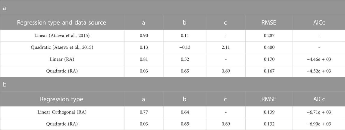
TABLE 2. Coefficient correlation parameters (a, b, c) that correspond to linear and quadratic regressions of the forms $M_{w} = {a * M}_{d} + b$ and $M_{w} = {a * M}_{d}^{2} + {b * M}_{d} + c$ , respectively; RMSE and AICc of these regressions are in respect to earthquakes located within RA; a) The regression coefficients of Ataeva et al. (2015) are from S-wave analysis and the magnitude range of $2.7 \leq M_{d} \leq 5.6$ , and were achieved through Eqs 1–3 (see Methods section); b) Comparison between orthogonal regression and quadratic OLS regresion.

In Figure 3, we compare between two OLS regressions, linear and quadratic, finding a relatively lower RMSE values obtained by the OLS quadratic fit (Figure 3C) compared with the linear OLS fit (Figure 3A). The parameters retain stable residuals around zero throughout the entire magnitude range for both regression types (Figure 3B, D). However, both the lowest and highest magnitude ranges suggest that the quadratic fit (Figure 3D) shows more constrained convergence around the line y=0 in comparison to some bias in the linear fit (Figure 3B). In addition, the total RMSE of the quadratic fit is slightly smaller (Table 2), and also the AICc method (Hurvich and Tsai, 1989), based on the Akaike Information Criteria (Akaike, 1974), shows lower values for the quadratic fit (Table 2). We also examined a linear orthogonal regression (OR), comparing it to the quadratic OLS fit. The quadratic OLS has better fit, reflected in its lower RMSE and AICc values (Table 2).

FIGURE 3

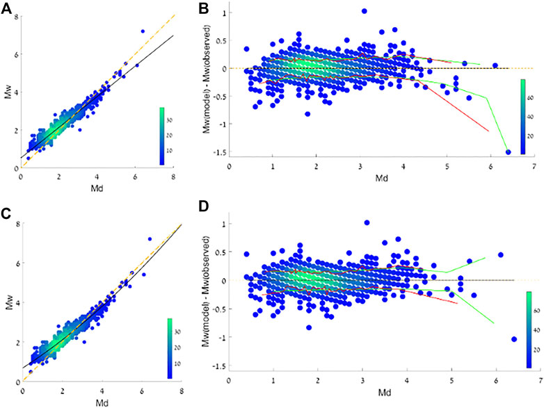
FIGURE 3. Linear and Quadratic fits of the current study, within the RA. Black lines in (A,C) are linear and quadratic fits, respectively, within RA, superimposed on the associated earthquake data. Dashed yellow lines represent 1:1 ratio. Residuals from these fits are scattered for the linear (B) and quadratic (D) fits; where the black line is the linear fit of these residuals, dashed yellow line represents 1:1 ratio; Green and Red lines show the detailed RMSE in intervals of 25 events in an ascending order of magnitudes, and in intervals of a single magnitude, respectively, calculated separately for the negative and positive residuals.

The stability of the regressions and corresponding residuals with detailed RMSE were also tested for earthquakes within NCA (Supplementary Figure S1), showing similar results (Table 2; Supplementary Table S1). For a more robust conversion that is based on a larger number of earthquakes, we choose to use the parameters obtained by the entire research area (RA); hence, our M_d to M_w conversion formula (Table 2) is:

M_{w} = 0.03 {* M}_{d}^{2} + 0.65 {* M}_{d} + 0.69 (5)

4.2 The magnitude of completeness and the b-value

The magnitude of completeness (M_c) is the minimum magnitude of which the seismic network detects all the events. Therefore, it marks the point from which the frequency-magnitude distribution is linear. We apply a few algorithms, by Goebel et al. (2017), following Aki (1965) and Clauset et al. (2009), based on Kolmogorov-Smirnov test, and by Mizrahi et al. (2021), is also based on Clauset et al. (2009), deducing M_c with high statistical robustness. Both algorithms suggest a completeness magnitude of 2.1 for the NCA. Similarly, in a previous work (Sharon, 2020), M_c was estimated as 2.0 for the NCA, for the years 1983–2017. This is in consent with prior estimations of Shapira (1992), obtaining M_c = 2.0 for a region, approximately overlapping the NCA, between the years 1984–1991. The predominant (or even the only) magnitude type in the analyses of Sharon (2020) and Shapira (1992) was M_d. Our conversion formulation (Eq. 5) indicates that M_d=2.0 is approximately equivalent to M_w of 2.1. Thus, we conclude that the magnitude of completeness for our homogenised catalogue is 2.1. As the NCA dataset is the one used later for more detailed analysis, by plotting the moment magnitude as a function of the sequential number of events (e.g., Zhuang et al., 2017; Bustos et al., 2022), we demonstrate that there are no clear short-term periods of magnitude incompleteness, within the NCA dataset (Figure 4).

FIGURE 4

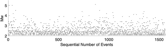
FIGURE 4. Moment magnitudes arranged by the sequential number of events. Mw is set to the obtained magnitude of completeness, Mc=2.1, demonstrating that there is no clear short-term magnitude incompleteness in the data used for the following analysis, within the network coverage area (NCA).

In general, higher M_c is expected for remote seismicity for which the seismic sensitivity decreases. This is demonstrated for earthquakes recorded in the entire research area (RA), where both algorithms of Goebel et al. (2017) and Mizrahi et al. (2021) suggest that M_c = 3.8.

We calculate the b-value through the Maximum Likelihood Estimation by the following equation (Marzocchi and Sandri, 2003; following Fisher, 1950; Utsu, 1966; and Bender, 1983):

b = \frac{1}{\ln [10] [\bar{M} - (M_{c} - ∆ M / 2)]} (6)

where $\bar{M}$ is the sampling average of the magnitudes, M_c is the completeness magnitude, and $Δ M$ is the magnitude bin interval in which the data is examined. The standard error of the b-value is obtained from the following formula (Shi and Bolt, 1982):

σ_{b} = 2.30 b^{2} {(\sum_{i = 1}^{n} {(M_{i} - \bar{M})}^{2} / (n (n - 1)))}^{0.5} (7)

where n is the number of earthquakes.

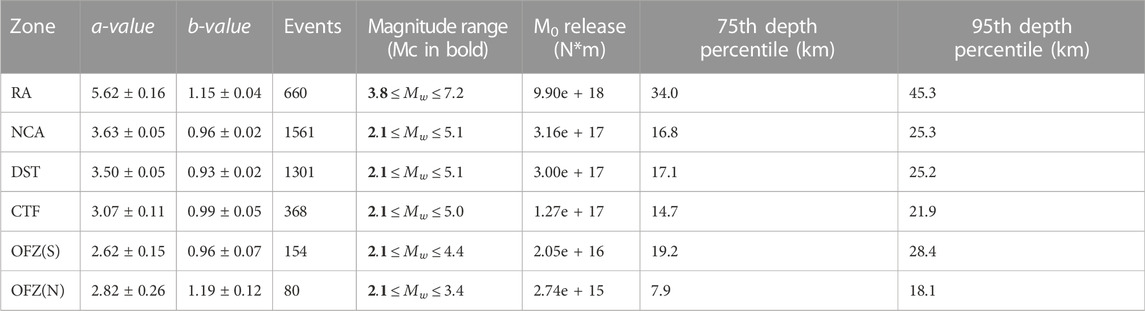
We calculate the frequency-magnitude parameters for several zones (Figures 5, 6): first, for regional zones: RA and NCA, and then for zones that differ in their local tectonics (Figure 5; Table 3). The zone of the DST is defined here by a ∼25-km width polygon representing the deformation zone of the southern section of the DST (excluding the Gulf of Elat due to the lack of seismic coverage). The width of the polygon increases up to 28-km in pull-apart basins, and decreases to 20-km at more localised sections that consist of long straight fault segments. For the rest of the NCA, the polygon of the CTF seismogenic zone (Sharon, 2020) is adopted to divide the off-fault seismicity into southern and northern Off-Fault Zones, OFZ(S) and OFZ(N), respectively (Figure 5). These two zones are also bounded by the DST polygon from the east and hence reflect two local tectonic provinces (Neev et al., 1976; Ben-Avraham and Ginzburg, 1990; Sadeh et al., 2012) that are separated from the main active fault zones. The frequency-magnitude parameters are presented in Table 3 for each of these tectonic zones (Figure 5), and their detailed plots are provided in Figure 6. In addition, the frequency-magnitude parameters of the seismogenic zones (Sharon, 2020) are provided in Supplementary Table S2.

FIGURE 5

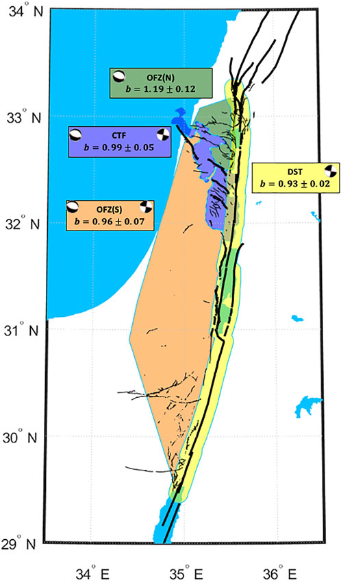
FIGURE 5. Tectonic zones and their b-values, within the NCA. DST is in yellow, CTF is in purple; Off Fault Zones (OFZ) have two sections: south [OFZ (S), in orange], and north [OFZ (N), in green] of the CTF, differing in their prevailing style of faulting. Note the partial overlap between DST and both CTF and OFZ (N). Bold and thin black lines are the main seismic sources and Quaternary faults, respectively (Sharon et al., 2020). Also shown are focal mechanism diagrams, demonstrating the dominant style of faulting in each tectonic zone, inferred from geological, seismological and geodetic observations (see text for further details).

FIGURE 6

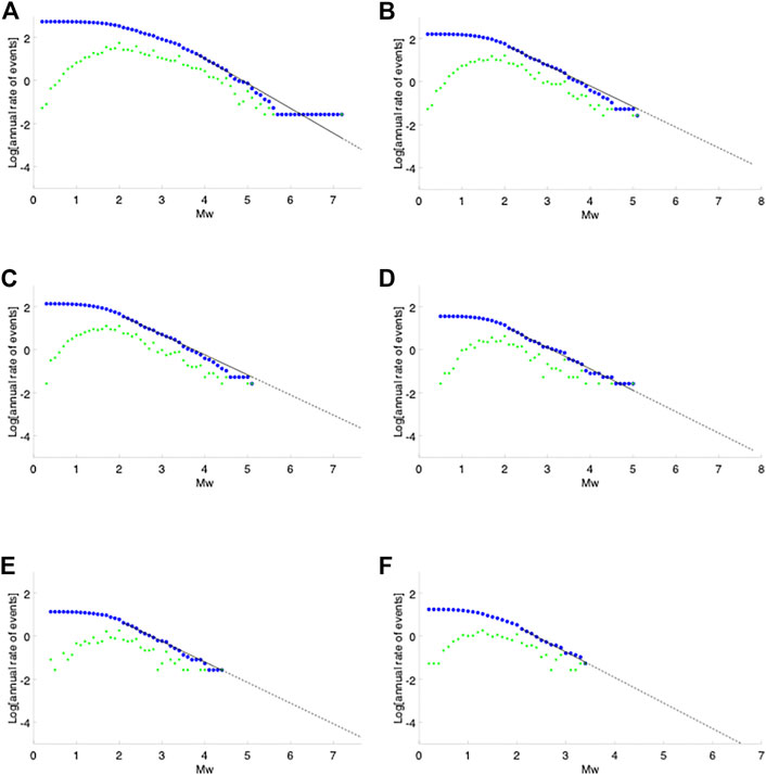
FIGURE 6. The frequency-magnitude relation for all earthquakes recorded between 1983 and 2020, within (A) RA; (B) NCA; (C) DST; (D) CTF; (E) OFZ (S); (F) OFZ (N). Dashed parts are extrapolations. Note that the y-axis marks the annual rate of seismicity, and not the total number of events. The tectonic zones of sub-plots c–f are presented in Figure 5.

TABLE 3

TABLE 3. Seismic characteristics of tectonic zones (Figures 4, 5).

5 Variations of the b-value

5.1 Spatial variations of the b-value

We first examine whether the differences in the b-values between the tectonic zones (Table 3; Figure 5) reflect different style of faulting. We examine only the tectonic zones, within the NCA, all affected by a similar network coverage, reflected also by similar magnitude of completeness values of Mc=2.1 (Figure 5). The strike-slip dominated DST (Garfunkel, 1981, 2014; Hofstetter et al., 2007; Marco and Klinger, 2014) shows a b-value of 0.93. The CTF zone, which accommodates an extensional and strike-slip associated deformation (Freund, 1970; Achmon, 1986; Rotstein et al., 1993; Hofstetter et al., 1996; Sadeh et al., 2012), has a b-value of 0.99. The Galilee area, marked by OFZ(N), is mostly extension-dominated normal faulting (Freund, 1970; Ron et al., 1984; Hofstetter et al., 2007), and shows a b-value of 1.19. The OFZ(S), an area of sparse seismicity associated with strike-slip and extensional structures (Bentor and Vroman, 1954; Bartov, 1974; Zilberman et al., 1996; Avni et al., 2000; Ginat et al., 2000, 2002), shows a b-value of 0.96. These b-values, including their errors (Shi and Bolt, 1982), show a subtle preference of higher b-values for extensional faulting. This trend is most prominent for the OFZ(N) (Figure 5) with a b-value of 1.19. We further explore the significance of this trend through two statistical methods: the Utsu’s method (Utsu, 1999; e.g., Xie et al., 2019) and the Student’s t-test (Gosset, 1908; e.g., Petruccelli et al., 2018). 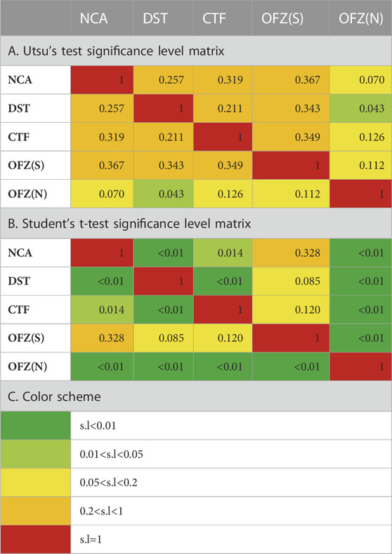In both methods, we test the statistical significance for ten pairs, comprising the relations between the five tectonic zones (including the “parent” NCA zone), and present the results by significance level matrices (Table 4), in which the significance level ( $s . l .$ ) is between 0 and 1; $s . l . < 0.01$ is highly significant and $s . l . = 1$ indicates identical datasets (e.g., Utsu, 1999).

TABLE 4

TABLE 4. Analysis of statistical significance for the Tectonic Zones, showing the significance level ( $s . l .$ ) matrices according to a) Utsu’s test; and b) the Student’s t-test. The statistical significance follows a color scheme (Table 4c) defined by the range of $s . l .$ , in which the green shades show $s . l . \leq 0.05$ threshold required for obtaining statistical significance. While the Utsu’s test show high similarity between the datasets, and therefore except for one pair (DST ←→OFZ(N)) does not indicate statistical significance, the Student’s t-test shows that seven out of 10 pairs are significantly different from each other, with $s . l . \leq 0.05$ . The stages of calculation for the t-test are provided in the Tables A3 and A4 of the Supplementary material.

In Table 4 we present the results obtained by Utsu’s method. In this method, we first compute the AIC (Akaike Information Criteria; Akaike, 1974) for each examined dataset. Then the difference between each dataset-pair ( $Δ A I C$ ) is calculated for each dataset, and the significance level is given by the probability $P = e^{(- \frac{Δ A I C}{2}) - 2}$ (Utsu, 1999); when p $\leq 0.05$ the two examined datasets are significantly different. According to Utsu’s method only one pair shows clear statistical significance (DST←→OFZ(N); Table 4). In Table 4 we present the results obtained by the Student’s t-test method. The type of t-test is chosen according to the ratio between each pair’s b-value standard deviations, $σ_{1} / σ_{2}$ (Rice, 2006) defining whether the variances of the b-values are similar or not between two tectonic zones (Supplementary Table S3). By setting the statistical significance requirement to $s . l . < = 0.05$ (e.g., Utsu, 1999) and by using the Student’s t-distribution table (Supplementary Table S4), we determine whether the observed differences between the b-values of two tectonic zones are statistically significant or a matter of chance, hence insignificant (Table 4). In addition to Utsu’s method, the Student’s t-test method suggests that except for the OFZ(S) related pairs, all the other pairs are significantly different from each other, meaning that the differences between the b-values are not randomly distributed. Hence, they may be attributed to physical causes, such as the predominant faulting style (Schorlemmer et al., 2005). Such differences between the two methods have been observed, for example, by Petruccelli et al. (2018), as the Student’s t-test method has shown more dataset-pairs with statistical significance than the Utsu’s method, for all the intermediate cases (those that do not reflect a pure faulting style; see Tables 3, 4 in Petruccelli et al., 2018).

5.2 Spatial variations of the b-value along the DST

We further explore in detail the spatial variations of the b-value along the main tectonic feature, within the DST polygon (Figure 5), by systematically scanning it in a 60-km long latitudinal bands, at 1-km increments, using the DST’s polygon completeness level of M_c=2.1 (Table 3; Supplementary Figure S2). These spatial bands represent the approximate minimum length to capture at least 100 events at each sample, with only one gap in between the bands (Figure 7). The b-value and its error (Shi and Bolt 1982) are calculated at each sample, where the mean number of events in these spatial bands is 185. An additional sparse-seismicity profile (50–99 events per sample; Figure 7) aligns with the main profile, showing a consistent behaviour of the b-value profile along the DST. In addition, the error bar band around the profile shows that the changes in the b-value are significant, substantially larger than the errors. The same spatial profiling is generated for the 75th and 95th hypocentre depth percentiles, and for the accumulated seismic moment converted from the magnitudes (Figure 7). The depth percentiles mark the depth profiles for which 75% and 95% of the events within the spatial bands are shallower, respectively. The accumulated seismic moment, which is the sum of seismic moments of all events within the spatial bands, is calculated at each sample.

FIGURE 7

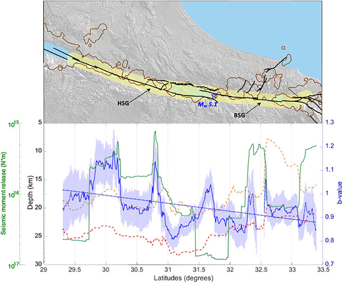
FIGURE 7. Top part: Map showing the DST polygon (yellow), defining the data for the analysis. The black lines show the main sources (see Sharon et al., 2020). Bottom part: Spatial variations of the b-value (in blue), of the 75th and 95th hypocentre depth percentiles (dashed yellow and red lines, respectively) and of the cumulative seismic moment release (in Green). Note the left axes are directed downwards. Solid and dashed lines of the b-value indicate at least 100 events, and 50–99 events per sample, respectively, and are shown with their light blue error bar band surrounding them; the blue linear dashed curve marks the spatial trend of the b-value. Within the Top part, the brown polygon marks zones with high values of seismic density and seismic moment density (see Sharon et al., 2020), overlapping the DST polygon. These zones emphasize two seismic gaps: 1) HSG—Hazeva Seismic Gap (latitudes ∼30.7°–30.8°N), and 2) BSG—Beit She’an Seismic Gap (latitudes ∼32.4°–32.6°N); the latter is prominent enough to also leave a gap within the b-value profile (Bottom Part).

The profiles presented in Figure 7 show rather complex correlations between the b-value and both the seismogenic depth and seismic moment release. We observe an inverse correlation of the b-value with the seismogenic depth along the DST, with lower b-values for deep seismogenic zones (i.e., latitudes 30.3°–30.7°, 30.9°–31.3°). A similar trend is presented in Supplementary Figure S3) for the tectonic (Figure 5) and seismogenic zones (Sharon, 2020; provided also in the Supplementary Figure S4). In addition, the seismic moment release shows at the southern section an inverse correlation with the b-value (latitudes 29.3°–31.0°; Figure 7); for example, this is emphasized at the “quasi-spike” of the b-value in latitude ∼30.8 $°$ . In contrast, the b-value increase at ∼31.7 $°$ , cannot be clearly correlated either to the seismogenic depth or to the seismic moment release, and seems to correspond to the M_w 5.1 mainshock (Hofstetter et al., 2008) with its aftershock sequence (see Figure 7A). This increase may reflect delocalization at the northern Dead Sea basin associated with its structural complexity (e.g., Garfunkel and Ben-Avraham, 1996). Yet, with all the complexity of the b-value profile, the overall trend shows that the b-value decreases northward along the DST (dashed blue linear trend line in Figure 7).

5.3 Temporal variations of the b-value along the DST

Since the relationship between the b-value and the seismic moment release has not been comprehensively studied, it is not clear whether the inverse spatial correlation (southern section, Figure 7) is a typical relationship, or whether it is biased by specific significant seismic activity (e.g., mainshocks, aftershocks, swarms). Therefore, some insights may be obtained by examining the temporal relations between the b-value and the seismic moment release. Statistical methods have been developed for examining high-resolution temporal variations of the b-value (e.g. Wiemer et al., 1998; Mousavi et al., 2017). However, applying them requires focusing on specific sub-zones, reducing to too small datasets in the case of the DST, due to the relatively low-intensity seismicity. Therefore, we investigate the temporal correlation of the b-value with the seismic moment release (Figure 8), by applying a rather simple technique, calculating the b-value in a moving time window, with a fixed number of 100 events per window, and a time interval of five events; also here, the DST’s polygon completeness level of M_c 2.1 is applied (Table 3; Supplementary Figure S5). Similar temporal analysis of the b-value, using a fixed number of events, has been shown and discussed in other studies (e.g., Nuannin et al., 2004; Tormann et al., 2013). In addition, as the catalogue consists of earthquakes recorded continuously by the ISN, we assume the data is inherently homogenous, with no temporal bias that can be caused by data comprising a combination of different catalogues (e.g. Zúñiga and Wiemer, 1999; Tormann et al., 2010).

FIGURE 8

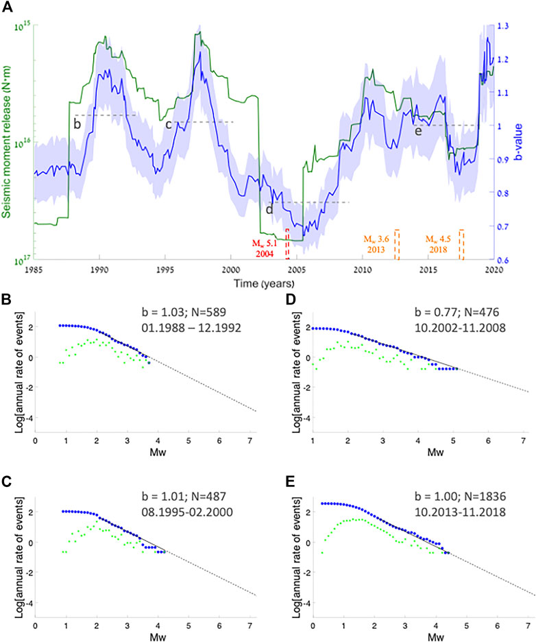
FIGURE 8. (A) Temporal variations of the b-value (in blue) with their light blue error bar band around them, and of the cumulative seismic moment release (in green; note the axis on the left is directed downwards) in the DST (Figures 5, 7), based on 100-event time windows in 5-event intervals. Also marked are the b-values calculated for specific time-windows [(B–E); dashed grey lines], verifying the fluctuations seen in the b-value profile; their frequency magnitude curves are presented in panel 8 (B–E). Two reductions of the b-value can be related to swarm activities at the Sea of Galilee, during 2013 and 2018 (dashed orange rectangles; Wetzler et al., 2019).

The temporal analysis (Figure 8) mainly shows an inverse correlation between the b-value and the seismic moment release (Figure 8A). We also examine the b-value in specific time windows, with a minimum of 450 events per time window, achieving higher statistical confidence. Their frequency-magnitude plots are presented in Figures 8B–E. These time-windows deduce b-values that fit the fluctuating b-value profile obtained by the fixed-amount-of-events method.

6 Discussion

6.1 Relation to the differential stress and faulting mechanism

The seismogenic depth along the DST fluctuates correlatively with the thermal profile (Shalev et al., 2013; Wetzler and Kurzon, 2016). The >25-km deep seismicity in some parts (Figure 7), particularly in the Dead Sea basin, indicates a cold crust with a deep brittle-to-ductile transition zone (Aldersons et al., 2003; Shalev et al., 2013; Aldersons and Ben-Avraham, 2014; Wetzler and Kurzon, 2016), whereas shallow brittle-to-ductile transition occurs in zones of shallower seismogenic depth. The differential stress within the brittle crust increases with depth (e.g. Sibson, 1974, 1984; Llana-Fúnez and Lõpez-Fernández, 2015) as the confining pressure grows (Byerlee, 1968). Hence, deeper seismogenic zones are associated with higher differential stress because they include deeper portion of earth’s (brittle-) crust. We therefore interpret the inverse correlation between the b-value and the seismogenic depth (Figure 7) as related to the differential stress within the brittle crust. This interpretation is consistent with previous laboratory (Amitrano, 2003) and seismic observations (Gerstenberger et al., 2001; Spada et al., 2013; Scholz, 2015; Petruccelli et al., 2019b), which showed inverse correlation between the b-value and the depth of earthquakes, and hence with their corresponding differential stress.

The increase of the b-value in tectonic zones, as the predominant faulting style changes from strike-slip dominated DST to normal faulting dominated OFZ(N) (Figure 5), is interpreted here as another expression of the inverse dependency of b-value with differential stress environments (Schorlemmer et al., 2005; Llana-Fúnez and Lõpez-Fernández, 2015; Petruccelli et al., 2019b). This relation is shown by normal faults that are associated with relatively lower differential stresses and higher b-values, while strike-slip faults that are associated with higher differential stresses, and lower b-values.

We also observe an overall trend of the b-value decreasing northwards, within the DST polygon (Figure 7). This trend may be caused by variations of mechanical parameters such as the internal friction angle and faulting geometry (Amitrano, 2003; Petruccelli et al., 2019a). Such variations can be linked to geometrical changes of the plate boundary (Garfunkel, 1981; Joffe and Garfunkel, 1987) and perhaps a transition from the extensional pull-apart basins of the Gulf of Elat (Reilinger et al., 2006) in the southern end of the DST polygon, closer to the Red Sea rift, to the transpressional LRB in the north (Gomez et al., 2007; Weinberger et al., 2009). Differences in the differential stress associated with these structural variations may also be related to post-Neogene widening of the fault zone along the southern section of the DST in the study area (latitudes<31°; Figure 7), while its northern section (latitudes>33°; Figure 7) underwent convergence and shortening (Avni et al., 2000; Marco, 2007; Weinberger et al., 2009; Garfunkel, 2010).

6.2 The b-value and the seismic moment release

The b-value shows an inverse correlation with the seismic moment release, at least in the southern section of the DST (latitudes<31°; Figure 7), and a clearer inverse correlation is seen in the temporal analysis (Figure 8). The inverse correlation aligns with the theoretical study of Wyss (1973) and with observations from other tectonic domains (e.g., Cao and Gao, 2002; Bora et al., 2018).

Seismic moment release is affected by two main factors: the accumulation of seismic moment of small events, and the addition of seismic moment from more significant events. The latter, when exists, tends to dominate over the former. In many aftershock sequences it has been observed that the b-value increases (Suyehiro, 1966; Gibowicz, 1974; King, 1983; Wiemer and Katsumata, 1999; Gulia et al., 2018), due to the stress relaxation after the mainshock and activation of fault branches at the periphery of the rupture, while some have shown a decrease in the b-value around the mainshock (e.g., Mukhopadhyay et al., 2013). A decrease in b-value prior to the main shock has been observed in other studies, and was associated to an increase of the differential stress (e.g. Schorlemmer and Wiemer, 2005; Rivière et al., 2018).

In the case of the DST, the seismicity observed here is within magnitudes of up to M_w 5.1, consisting of: one significant mainshock of M_w 5.1 in 2004 at the Dead Sea basin, two swarms at the Sea of Galilee of M_w ∼3.5 and ∼4.5, in 2013 and 2018, respectively, and sporadic seismicity of up to M_w 4.4, throughout the DST. Except for the swarms, which show a clear decrease of the b-values (Figure 8), all the main shocks, including the M_w 5.1, are characterised by a relatively short aftershock activity (Hofstetter et al., 2008); for the M_w 5.1 event, the complete aftershock sequence includes 23 events above the M_c of 2.1. The b-value spatial peak, corresponding to this sequence in the spatial b-value profile (Lat ∼31.7; Figure 7), is not aligned with the spatial seismogenic depth profile and the spatial seismic moment release profiles. Therefore, it seems that the temporal variation of the b-value within the DST mainly reflects the effect of moderate seismicity (M_w 3–5) on the whole size distribution, a phenomena that has been observed particularly in small datasets (Marzocchi et al., 2020), and in this case - with low aftershock activity. For the swarms (Figure 8), the reduction in the b-value reflects the repetition of similar size mainshocks, typical for swarms (e.g., Goebel et al., 2016, Wetzler et al., 2019).

6.3 Seismic gaps along the DST

Some of the sections along the DST, which show extremely low seismic activity, were documented by Sharon et al. (2020). The most prominent ones (Figure 7) are the Hazeva Seismic Gap (HSG) and the Beit She’an Seismic Gap (BSG). The HSG contains a “quasi-spike” b-value rise, which correlates to a rather similar “quasi-spike” of low seismic moment release (Figure 7). Since high b-values also relate to weak zones that may be associated with creeping (Schorlemmer et al., 2004; Wyss et al., 2004; Tormann et al., 2013, 2014), the combination of a high b-value with low seismic activity implies that local creeping occurs in this zone. Geodetic data from the BSG has been interpreted to show shallow crustal creep (1.5 ± 1.0 km) in its northernmost part (Hamiel et al., 2016). Sharon et al. (2020) suggested that the relative absence of seismicity in this gap is caused by slip partitioning of the DST activity to the CTF (Sadeh et al., 2012; Hamiel et al., 2018), and to some extent, shallow creeping. Assuming the low b-value in the southern part of the BSG is not an artefact of the small amount of data, it may indicate a particularly locked section (e.g., asperity; Wiemer and Wyss, 1997, 2002; Wyss, 2001; Spada et al., 2013; Tormann et al., 2014). The sparse seismicity observed here and the relative quiescence along the segment in the past centuries, as well as the associated large displacement deficit (Marco and Klinger, 2014; Lefevre et al., 2018), should be accounted for in seismic hazard assessment.

6.4 Comparison to other continental transform plate boundaries

Comparison of b-values between different tectonic domains may be problematic, since some factors can dramatically affect the b-value: the magnitude type (Wyss, 2020) and its calibration (Tormann et al., 2010), changes in the network operating procedures (Zúñiga and Wiemer, 1999), the spatial frame (e. g., Page and Felzer, 2015), and the time window in respect of the seismic cycle (e.g., Raub et al., 2017); that is, assuming a correct choice of the completeness magnitude and well-calculated b-value (i.e., the method used). Thus, although the b-value is expected to vary between regions according to the faulting style (Schorlemmer et al., 2005), such interpretations between different faults of different regions should be made carefully. Here, we compare our results, regarding the DST, with three other major continental transform fault systems (e.g., Gauriau and Dolan, 2021).

A b-value of 1.03 was deduced for a 20-km width spatial zone surrounding the southern San Andreas fault (Page and Felzer, 2015). Rather similar b-values were achieved in a wider zone (0.99–1.01; Hutton et al., 2010). Two zones, comprised of widths of 10 and 20 km off the northern part of the San Andreas fault, California, yielded b-values of 0.99 and 0.93, respectively (Wyss, 2020). In New Zealand, a b-value of 0.98 was obtained for a 20-km wide zone along the central Alpine fault (Wyss, 2020), which accommodates reverse slip rates of approximately 20–40% of its horizontal motion (Norris and Cooper, 2001). A larger zone surrounding the central Alpine fault deduced a b-value of 0.85 (Michailos et al., 2019). Seismicity from the area of the North Anatolian fault, Turkey, divided into three parts, yielded b-values of 1.01–1.02 in its eastern and central parts, and 1.13 in the western part (Öztürk, 2011).

Our results indicate a b-value of 0.93 for the DST with a gentle spatial trend associated with tensional and compressional components in the edges of the study area. Considering that the northern part of the San Andreas fault is somewhat affected by a compression regime (e.g., Schwartz et al., 1990; Williams et al., 2006), and that the western part of the North Anatolian fault accommodates normal faulting components (Reilinger et al., 1997), their corresponding b-values imply also a gentle faulting-style dependency of the b-value, similar to our DST observations. In addition, the b-value of the DST is somewhat lower compared with these other major strike-slip faults, despite reverse component in parts of the San Andreas fault and particularly in the Alpine fault. This might be due to relatively deeper seismicity of the DST (up to 21–27 km), in comparison to the other examined faults, possibly associated with increased differential stress along significant parts of the DST.

7 Conclusions

We analyse ∼20,300 earthquakes along the DST and its periphery and provide a new conversion formula from $M_{d}$ to $M_{w}$ . After converting magnitudes, we determine the frequency-magnitude parameters for the complete catalogue, and to five significant subsets. Our b-value results align with previous studies in the region (Salamon et al., 1996; Shapira and Hofstetter, 2002; Hamiel et al., 2009; Lu et al., 2020), providing a high resolution characterisation of the frequency-magnitude statistical parameters, including within well-defined tectonic zones, consisting the network coverage area.

Variations of the b-value within the tectonic zones correspond to changes in the tectonic regime and presumably to the associated style of faulting, with values that vary from 0.93 in the strike-slip dominated DST to 1.19 in the normal faulting dominated OFZ(N)). In addition, high-resolution spatial profile along the DST reveals a decreasing trend of the b-value towards the north. This trend corresponds to a possible increased differential stress associated with a gradual change in the faulting regime, from an extension component at the south, where the DST shifts from the extensional pull-apart basins of the Gulf of Elat, closer to the Red Sea rift, to a compression component at the north, approaching the LRB. Hence, we propose that these variations reflect the inverse dependency of the b-value with the differential stress as revealed from the Anderson (1905) theory of faulting.

The DST spatial profile reveals an inverse dependency between the b-value and the seismogenic depth as the b-value decreases with the deepening of the seismogenic depth. Considering that deeper seismogenic zones are distributed over depths of higher differential stress, we suggest that this inverse correlation results from variations in the differential stress, which increases with depth within the brittle part of the crust, showing rheological dependency of the b-value.

Our analyses show that within the DST zone, the b-value inversely correlates with seismic moment release, reflecting a weak role of aftershocks within the DST. While the temporal fluctuations of the b-value better reflect this correlation, its spatial variations are linked to both the seismic moment release and the seismogenic depth.

The observations from this study are in line with previously-suggested dependency between the b-value and the differential stress (Scholz, 1968, 2015; Amitrano, 2003; Goebel et al., 2013). Considering this dependency and associated previous observations, we also suggest that anomalous b-values may indicate creeping and locked sections of the fault in two seismic gaps defined here—the Hazeva and Beit She’an seismic gaps, respectively. Our results contribute to the seismo-tectonic understanding of the DST, and should also be considered for seismic hazard evaluation in the region. In addition, as the observed spatio-temporal relations between the b-value and the seismic moment release are not well understood, this relation should be further investigated in higher resolution, and when more detailed data will be available for the region.

7.1 Data and resources

The seismic catalogue used in this study is an updated relocated catalogue, based on what was presented in Wetzler and Kurzon, 2016, and can be downloaded at: <https://www.gov.il/en/Departments/General/seismic-catalogs-files>. Maps were generated using QGIS open source mapping software [(<https://www.qgis.org/>), last accessed November 2022], and the global high resolution population GIS layers were downloaded from <https://www.worldpop.org/>. Many of the figures were generated by Matlab (<https://www.mathworks.com/products/matlab.html>), last accessed November 2022, and all figures were finalized using Microsoft PowerPoint. Naturally, we cannot cover all aspects in the main manuscript, and accordingly, we have added a Supplemental Material section, providing more details and additional supporting analyses.

Data availability statement

Publicly available datasets were analyzed in this study. This data can be found here: https://www.gov.il/en/Departments/General/seismic-catalogs-files.

Author contributions

MS and IK contributed to the conception and the design of the study. MS and IK performed the majority of the data analysis. MS and NW performed additional data analysis. MS wrote the first draft of the manuscript. IK and NW wrote sections of the manuscript. AS and SM provided essential geological and geophysical insights. All authors contributed to manuscript revision, read, and approved the submitted version.

Funding

This study was supported by the Ministry of Energy grants: 214-11-10, 219-11-054 and 222-11-001.

Acknowledgments

We thank Andrey Polozov, Ran Nof, Marina Gorstein, Yuval Tal, Yariv Hamiel and Marcelo Rosensaft for their assistance and their useful comments. We thank the guest associate editor, Guido Adinolfi, and two reviewers for their helpful comments, assisting us in improving the manuscript.

Conflict of interest

The authors declare that the research was conducted in the absence of any commercial or financial relationships that could be construed as a potential conflict of interest.

Publisher’s note

All claims expressed in this article are solely those of the authors and do not necessarily represent those of their affiliated organizations, or those of the publisher, the editors and the reviewers. Any product that may be evaluated in this article, or claim that may be made by its manufacturer, is not guaranteed or endorsed by the publisher.

Supplementary material

The Supplementary Material for this article can be found online at: https://www.frontiersin.org/articles/10.3389/feart.2022.1074729/full#supplementary-material

References

Achmon, M. (1986). The Carmel border fault between yoqneam and nesher. M.Sc. thesis. Jerusalem: Hebrew University of Jerusalem.

Agnon, A. (2014). “Pre-instrumental earthquakes along the Dead Sea rift,”in Dead Sea transform fault system: Reviews. Editors Z. Garfunkel, Z. Ben-Avraham, and E. Kagan (Dordrecht: Springer Netherlands), 207–262.