 Shatakshi Verma
 Shashi Kumar
 Varun Narayan Mishra
 Rahul Raj3
- 1Centre for Climate Change and Water Research, Suresh Gyan Vihar University, Jaipur, India
- 2Photogrammetry and Remote Sensing Department, Indian Institute of Remote Sensing (IIRS), ISRO, India
- 3Institute of Bio- and Geosciences, Agrosphere (IBG-3), Forschungszentrum, Jülich GmbH, Germany
Polarimetric synthetic aperture radar remote sensing extracts the information about the target using decomposition models to separate the polarimetric information into single-bounce (contributed by smooth surfaces), double-bounce (contributed by urban structure), and volume (mainly due to vegetation cover) scattering components. The penetration capacity of the electromagnetic wave into the surface increases with the decrease in its frequency. This study explores and compares the polarimetric decomposition models for scattering-based characterization of land use and cover using multifrequency spaceborne synthetic aperture radar sensor datasets that were acquired over San Francisco, CA, USA. The present work compares the scattering parameters of coherent (Pauli), roll-invariant (Barnes), eigenvalue–eigenvector (Cloude), and compact-polarimetric (Raney) decomposition modeling approaches for scattering-based characterization of urban structures, waterbody, and vegetation cover. The land use/cover classification was performed based on the scattering response of the scatterers using a support vector machine classifier. The outputs of the classification approach on multisensor, multifrequency, and multi-polarization polarimetric synthetic aperture radar data have shown reasonable accuracy in classifying the land use and land cover. The decomposition models fail to characterize the oriented urban structures that cause misclassification of urban structures as vegetation. The higher-order roll-invariant decomposition modeling approaches could improve the interpretation of different targets and accuracy in land use and land cover classification.
Introduction
The development of polarimetric synthetic aperture radar (PolSAR) remote sensing has provided an opportunity to the scientific community and researchers to study the polarimetric properties of the objects on the Earth's surface (Schuler et al., 2003, Schuler et al., 2004; Sato et al., 2012; Chen and Sato, 2013; Chen et al., 2014a; Kumar et al., 2022). The PolSAR remote sensing is based on the concept of electromagnetic (EM) wave polarization. The polarization state of the EM wave is defined by the amplitude, orientation angle, ellipticity, and direction of the electric field vector. The PolSAR sensor emits the EM wave to the ground target in a specific polarization state. The target absorbs some EM energy and reradiates the rest of the EM energy as a new EM wave in a different state of polarization to the sensor. This change in polarization state depends on the shape, size, orientation, and dielectric property of the target (Lee and Pottier, 2009). Therefore, the study of polarimetric properties is essential for the characterization of different targets such as waterbody, buildings, bridges, and forest structures present on the Earth's surface, as each scatter produces a unique scattering response due to the differences in their dielectric and structural properties.
The PolSAR sensor can measure the scattering response of different types of scatterers within a single SAR resolution cell. The PolSAR sensor transmits the EM signal to the ground target in horizontal and vertical polarization mode and receives the backscatter signal horizontally and vertically, thus, providing the information in four polarimetric channels HH, HV, VH, and VV. It has been found that the polarimetric distortions present in the PolSAR data also affect the scattering retrieval contributed by different scatterers (Babu et al., 2021a, Babu et al., 2021b; Maiti et al., 2021). However, this is not a problem in recent days because concerned space agencies provide the data free from the polarimetric distortions, so the user should not get difficulty in accurate scattering retrieval from SAR data (Kumar et al., 2022). The polarimetric responses are sensitive to the dielectric and structural property of the imaged ground target. This polarimetric information can be decomposed into different scattering components such as surface/odd, double-bounce/dihedral, and volume, which describes the scattering mechanisms of the ground target. The odd-bounce scattering response is given by the smooth surfaces or Bragg's scatterers such as waterbody, double-bounce scattering response is produced by the high-rise buildings, and the volume scattering response is generated by the vegetation structures. These scattering components are useful for the characterization of the target within a single SAR resolution cell. Therefore, the decomposition of the PolSAR dataset is essential to retrieve the scattering information. There are various PolSAR-based (Cloude, 1985; Holm and Barnes, 1988; Krogager, 1990; van Zyl, 1993; Freeman and Durden, 1998; Yamaguchi et al., 2005; Freeman, 2007) and PolSAR Interferometry (PolInSAR)-based (Chen et al., 2014b; Agrawal et al., 2016; Shafai and Kumar, 2020; Bhanu Prakash and Kumar, 2021a; Bhanu Prakash and Kumar, 2021b) decomposition modeling approaches for extracting the scattering components from PolSAR datasets to study the different scattering mechanisms of the targets.
The decomposition modeling approaches are categorized as “coherent” and “incoherent,” “model-based” and “eigenvalue/eigenvector” based, and the decomposition based on the dichotomy of the “Kennaugh matrix (
The PolSAR sensor operates in the microwave region of the EM spectrum ranging from 1 mm to 1 m. These long-wavelength microwaves easily penetrate dust, smoke, and water vapor, which enable earth observation in all-weather conditions. The development of active SAR sensors brings the additional advantage that allows continuous monitoring of the Earth's surface, i.e., both day and night. There are different frequencies/wavelength bands used by the PolSAR sensor such as Ka—0.75–1.1 cm, K—1.1–1.67 cm, Ku—1.67–2.4 cm, X—2.4–3.8 cm, C—3.8–7.5 cm, S—7.5–15 cm, L—15–30 cm, and P—30–100 cm. Generally, the penetration capacity of the EM wave increases as the wavelength increases. Thus, each frequency band has their characteristic and applications. The longer wavelengths, such as L-band, can easily penetrate through the surface feature such as soil, ice, or forest canopy, which causes more interaction of emitted EM signal with the subsurface targets, branches, leaves, and tree trunks, and provide subsurface feature information. Therefore, the longer wavelengths are suitable for retrieval of subsurface information such as forest height estimation (Kumar et al., 2020), forest aboveground biomass retrieval (Kumar et al., 2019), mapping land subsidence (Ng et al., 2012; Chaussard et al., 2013), and archaeological studies (Stewart et al., 2013). The shorter wavelengths, such as X-band, have relatively less penetration capacity. The emitted EM wave interacts with the top layer of the soil, ice, or forest canopy and provides less subsurface information. Therefore, the shorter wavelengths are suitable for sea ice monitoring (Scheuchl et al., 2014), flood detection (Mason et al., 2010), oil spill observation (Velotto et al., 2011), and ship detection (Brusch et al., 2011).
In SAR remote sensing, the surface roughness is related to the wavelength used by the SAR sensor (
The scattering mechanism described by the radar target is greatly affected by its shape, size, and frequency or wavelength used by the SAR sensor (Ferro-Famil and Pottier, 2016). The scattering behavior of the target is determined by the ratio of the size of the target and the sensor's wavelength. Therefore, the sensitivity to the surface roughness decreases with an increase in the wavelength. The high-frequency or shorter EM wave can easily scatter from the surface, causing diffuse reflection, and low-frequency or longer EM wave easily penetrates through the surface, causing dominant specular reflection. Thus, an irregular surface may appear smooth in L-band, and a similar surface may appear very rough in X-band.
Many space agencies have launched radar satellites for the polarimetric-based study of the Earth's surface and subsurface features. National Aeronautics and Space Administration (NASA) was a pioneer to launch the first-ever synthetic aperture radar satellite “SeaSAT” in 1978. The SeaSAT's SAR sensor provided L-band HH polarization (HH
The classification of polarimetric datasets has gained wide attention due to its ability to measure the polarimetric response of the ground features. These polarimetric signatures in various polarization bases give a more detailed insight into radar targets (Jafari et al., 2015; Buono et al., 2017). Also, the development of polarimetric decomposition models has intensified its application in land use/land cover (LULC) classification because it provides scattering information associated with the ground targets (Alberga, 2007; Saito et al., 2018; Yin et al., 2018). A comparative study was done by Lardeux et al. (2009) using different polarimetric indicators derived from the decomposition of PolSAR datasets. The result showed that the support vector machine (SVM) algorithm outperforms the conventional Wishart classification approach. Another novel effort was made by Qi et al. (2012) for LULC classification. The combination of polarimetric decomposition and polarimetric SAR interferometric parameters was used to retrieve the information of textural and spatial features. A decision tree classifier was used for the classification. Bai et al. (2021) showed the improvement of the classification approach based on the integration of optical and SAR data to extract the urban and vegetation land cover feature. Niu and Ban (2013) significantly improved the classification accuracy using the polarimetric parameter of decomposition models derived from the multi-temporal SAR dataset.
Over the last few years, various classification methods based on statistical and nonstatistical approaches have been used to classify the Earth observation datasets (Lu, 2007; Kumar et al., 2015; Mishra et al., 2017a). Scientists are exploiting the machine learning approach for image classification practices (Mishra et al., 2017a; Yin et al., 2018, 2020; Chaudhary and Kumar, 2021; Rawat et al., 2021; Garg et al., 2022) due to its ability to handle multiple datasets and shows good accuracy in the classification results than other conventional approaches. Advanced machine learning-based classification algorithms such as SVM, artificial neural network, decision tree, and random forest have been extensively used for the LULC classification of satellite images (Kumar et al., 2015; Mishra et al., 2017b). The SVM algorithm has received substantial attention because of several advantages over the traditional classification method. It is sensitive to the dimensionality of the data accompanied by the size of training datasets (Pal and Foody, 2010; Kumar et al., 2015). It does not assume a probability distribution of the training datasets; as a substitute, it finds a decision from the training data directly based on a kernel function in a suitable space. The potentiality of the SVM method has attracted a great deal and is reported in many studies (Kumar et al., 2015; Kranjčić et al., 2019; Mishra et al., 2019; Orieschnig et al., 2021).
The scattering response of the target depends on the frequency used by the SAR sensor. A surface may appear rough in X-band; the high-frequency EM wave will easily scatter from the surface, causing diffuse reflection; a similar surface may appear smooth in L-band, as the EM wave easily penetrates through the surface, causing specular reflection. Therefore, it is necessary to study the unique polarimetric scattering response of radar targets such as waterbody, vegetation, and urban structure in different frequency ranges using fully polarimetric SAR datasets. The prime focus of this study is to compare the polarimetric parameters of decomposition modeling approaches for scattering-based characterization of LULC using multifrequency spaceborne SAR sensor datasets. The objectives of this study are as follows:
• extraction of the scattering components from multifrequency polarimetric SAR datasets using coherent (Pauli), roll-invariant (Barnes), eigenvalue–eigenvector (Cloude), and compact-polarimetric (CP) (Raney) decomposition modeling approaches.
• comparison of the scattering components of Pauli, Barnes, Cloude, and Raney decomposition models for characterization of the waterbody, urban, and vegetation structures.
• analysis of the accuracy of Pauli, Barnes, Cloude, and Raney scattering components for LULC classification using an SVM classifier.
Study Area and Datasets
The study site is located on San Francisco Peninsula on the west coast of the United States. This area is enclosed by the San Francisco Bay, Pacific Ocean, and the Golden Gate strait (Figure 1). The study site consists of natural and artificial features such as vegetation, forests, parks, buildings, roads, hilly terrain, ponds, and sea surface. The urban features of the study area illustrate both orthogonal and oriented urban structures. The orthogonal urban structure refers to the building structure that is orthogonal to the imagery. The oriented urban structure refers to the building structure oriented at some angle to the imagery. Therefore, the diversity of different land features of the study area is suitable for this work.
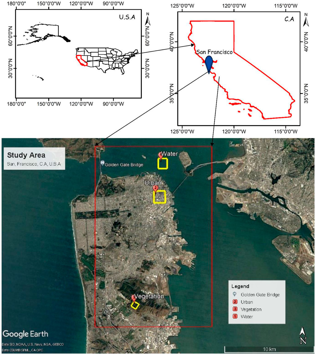
FIGURE 1. Location of study area: San Francisco, CA, USA, on Google Earth Image (historical optical imagery: April 9, 2008); subset of study area (red line); location of water, urban, and vegetation regions.
The objective of this work is the comparison of polarimetric parameters for the scattering-based characterization of LULC using multifrequency PolSAR datasets. The fully polarimetric multifrequency SAR datasets of the study area (San Francisco, C.A, United States) were not available for the same date. Therefore, this study utilizes multifrequency and multi-temporal fully polarimetric spaceborne SAR sensor datasets of ALOS-1 PALSAR-1, ALOS-2 PALSAR-2, RADARSAT-2, RISAT-1, Gaofen-3, and TerraSAR-X that were acquired over San Francisco, C.A, United States. The detailed description of datasets is given in Table 1.
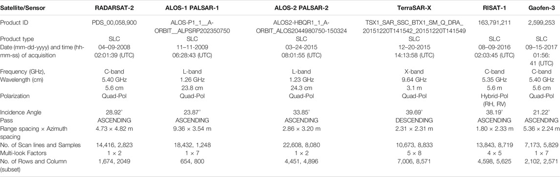
TABLE 1. Description of datasets: SLC—single look complex; Quad-Pol—HH, HV, VH, and VV.
Methodology
The PolSAR datasets were in single look complex (SLC) file format. The SLC SAR pixel represents the associated ground target information in the form of complex numbers—real and imaginary. Firstly, preprocessing (multi-looking, radiometric calibration, and terrain correction) of the polarimetric dataset was performed, then the coherency matrix was generated for polarimetric analysis. After that, scattering components were retrieved using Pauli, Barnes, and Cloude decomposition models on the coherency matrix elements derived from fully polarimetric datasets, and the
For this work, SNAP 8.0 software (SNAP 8.0 released—STEP, 2022) was used for the preprocessing of the polarimetric datasets; ArcGIS 10.5 software (ArcGIS Desktop Download and Documentation, 2022) was used for the geocoding: the coherency matrix generation. The polarimetric decomposition models were utilized using PolSARPro 6.0.3 software (PolSARpro v6.0 Toolbox Download—STEP, 2022). The accuracy assessment was performed using ENVI 5.3 software (ENVI, 2022). The ground reference data for the accuracy assessment were collected from Google Earth Pro version 7.3 (https://www.google.com/intl/en_in/earth/versions/#earth-pro). Figure 2 shows the methodological flowchart.
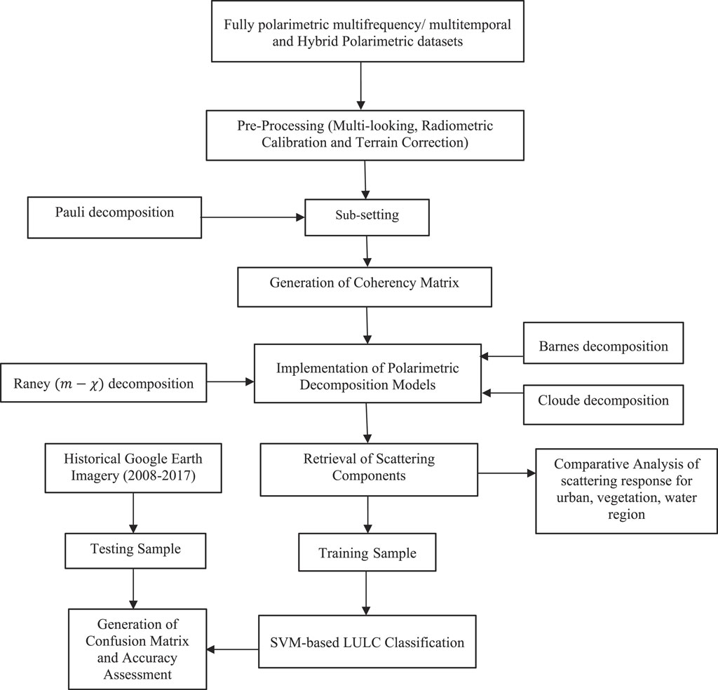
FIGURE 2. Methodology flowchart.
Data Preprocessing
The fully polarimetric multifrequency datasets were in SLC file format. The complex values of four channels—HH, HV, VV, and VH—are represented in a scattering matrix [S] (Eq. 1). In contrast, the CP sensor of RISAT-1 transmits the EM signal in the right circular mode, receives linear coherent backscattering response, and produces CP RH and RV datasets (Misra and Kirankumar, 2014; Babu et al., 2019b). The circular that transmits and linearly receives (CTLR) RH and RV datasets are expressed as complex scattering matrix [S] (Cloude et al., 2012) as of Eq. 2.
Here,
Because the datasets were in SLC file format consisting of slant-range ambiguity, the multi-looking was performed to generate the square pixels; the number of range-looks and azimuth-looks for each dataset is shown in Table 1. The multi-looking process also reduces the speckle noise from the SAR pixels. Then, radiometric calibration was done to remove the ambiguity from the SAR pixels that arise due to fluctuation in transmission and receiving of signal from the radar sensor or due to variation in satellite roll angle and the sensor records errors in the datasets. After that, terrain correction was performed on the radiometrically corrected datasets to eliminate the geometric distortions such as layover, foreshortening, and shadows, which generally occur due to variations in terrain surface height and tilt in SAR sensors position (Lillesand and Kiefer, 1979).
Polarimetric Synthetic Aperture Radar Coherency Matrix
In a subset of the study area comprising forest cover, vegetation, parks, and dense urban structures, the water surface was taken for further processing of the datasets (Figure 1). The details of the number of rows and columns used for the subset are shown in Table 1. A polarimetric coherency matrix was produced from the scattering matrix [S] (Eq. 1), which is based on the Pauli spin matrix. Considering the monostatic SAR system, the following Eq. 3 represents the Pauli feature vector corresponding to the ground target:
Here,
Here,
For the case of a single look CP SAR sensor system (Cloude et al., 2012), the CTRL datasets RH and RV are expressed as complex scattering matrix [S] as in Eq. 3. The stokes vector (
Here,
Here,
Polarimetric Decomposition Models
The polarimetric decomposition models aim to separate the PolSAR datasets into different scattering components. The decomposition models are broadly classified as coherent and incoherent. Pauli, Kroggager, Polar, and Cameron are the coherent decomposition models. The incoherent decomposition is classified as model-based and eigenvalue–eigenvector decompositions.
The model-baseddecomposition is based on fitting the physical scattering mechanism sub-models to the SAR observation to retrieve the scattering components (Freeman and Durden, 1998; Yamaguchi et al., 2005; Yamaguchi et al., 2006; Freeman, 2007; Bhattacharya et al., 2015). The scattering mechanism associated with the cloud of randomly oriented dipoles (such as forest canopy structure) is termed as volume scattering, the even-bounce or double-bounce response was produced by a pair of orthogonal surfaces with two different dielectric constants (such as building and bridges), the moderately rough or Bragg scatter describes the odd-bounce or surface scattering response, and the helix scattering response is associated to the “helix target.” The helix targets do not assume reflection symmetry in backscattering response and produce left- or right-hand circular polarization response for incident radar signal. Recently, two additional scattering mechanism models have been introduced for the oriented-dipole and compound dipole structures (Singh and Yamaguchi, 2018).
Huynen, Holms-Barnes, and Yang decompositions are based on the Kennaugh matrix “K” (Lee and Pottier, 2009). Huynen (1978) was the pioneer in developing the target decomposition theorems using PolSAR datasets. He proposed “phenological theory” to derive the radar scatterer's structural and physical properties. This theory aimed to isolate the radar backscattering response into a single residue target [i.e., the stationary or “pure target” (
Here,
The decomposition models are based on the eigenvalue–eigenvector of 3 × 3 Hermitian coherency
where
Here,
Pauli Decomposition
Pauli decomposition is coherent decomposition based on the Pauli spin matrix, as shown in Eq. 13. Here, the first element 1) corresponds to the odd bounce component associated with the smooth surface, the second elements 2) correspond to the double-bounce component associated with the corner reflectors such as walls and buildings, and the third 3) and fourth elements 4) correspond to the volume component associated with the forests or vegetations (Lee and Pottier, 2009).
where,
Considering the monostatic SAR system following the reciprocity principle,
The Pauli decomposition model was used on the scattering matrix [S] (Eq. 1), and
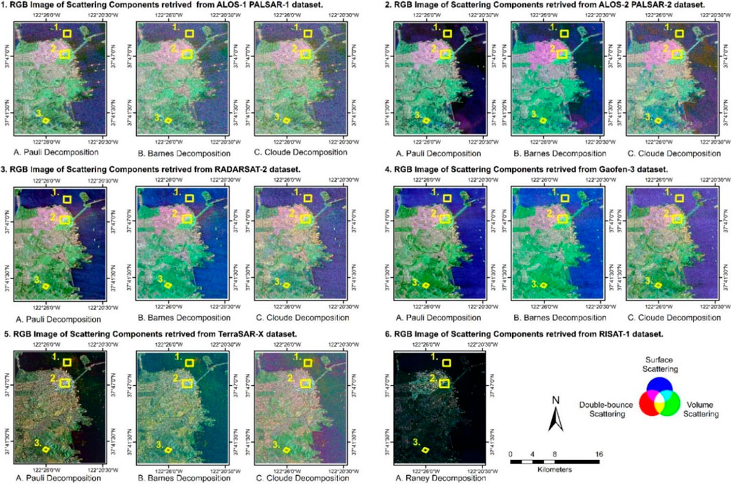
FIGURE 3. Scattering components retrieved from multi-temporal and multifrequency SAR sensor ALOS-1 PALSAR-1, ALOS-2 PALSAR-2, RADARSAT-2, RISAT-1, Gaofen-3, and TerraSAR-X datasets. Color composite RGB image of (A) Pauli, (B) Barnes, (C) Cloude scattering components: red-double-bounce scattering, green-volume scattering, and blue-surface scattering; Location of (1) water, (2) urban, and (3) vegetation regions for analysis of scattering response.
Barnes Decomposition
A roll-invariant decomposition technique was developed based on the Huynen N-target decomposition theorem (Lee and Pottier, 2009; Maghsoudi, 2011). Barnes objected to the theory of Huynen (1978), as the structural property derived from Huynen decomposition was not unique, and other decomposition techniques could present the same structural property. Hence, he proposed a generalized form of Huynen decomposition. The
Here, U (
Hence, the coherency matrix
•
•
The normalized target vectors
The Barnes decomposition model was used on the coherency matrix (Eq. 4) obtained in the previous step from fully polarimetric SAR datasets to retrieve the surface, double-bounce, and volume components. The RGB color composite image of the Barnes scattering components retrieved from multifrequency PolSAR datasets is shown in Figure 3.
Cloude Decomposition
Cloude (1985) made a significant approach for the retrieval of scattering elements based on the eigenvalue/eigenvector of the coherency matrix
Here,
Raney Decomposition
Raney et al. (2012) proposed the
Raneydecomposition was used on the 2 × 2 coherency matrix elements (Eq. 7) retrieved from the CP dataset to extract the surface→
Comparative Analysis of Scattering Response for Urban, Vegetation, and Water Surface
In this study, the mean pixel value of the surface, double-bounce, and volume scattering components derived from different decomposition modeling approaches were measured for the comparative study of scattering response for a waterbody, urban, and vegetation structure. Figures 1 and 3 show the location of the test area on the optical image of Google Earth and the color-coded RGB image of scattering components, respectively. The present work utilizes multifrequency PolSAR datasets of different sensors which were acquired on different dates between the years 2008 and 2017. The historical optical images provided by Google Earth were used for validation. The historical optical images of Google Earth were coordinated to the date of acquisition of SAR imagery for the validation of the test area selected for urban, vegetation, and water regions; there was a very minor or negligible change in the testing area during the span of 9 years (2008–2017). The test area for the waterbody represents the smooth surface. Such targets describe surface scattering response because the emitted SAR signal interacts with a single dielectric surface. The chosen urban test region comprises both orthogonal and oriented urban. The urban structure is termed as corner reflectors or dihedral structures that produce a double-bounce scattering response due to the interaction of transmitted SAR signals with two different dielectric media. The scattering response was measured for both orthogonal and oriented urban structures. The selected vegetation test region comprises distributed vegetation structure over undulating terrain. The vegetation or forest canopy are complex structures that produce a volume scattering response due to the interaction of SAR signal with multiple dielectric media such as branches, leaves, and tree trunks.
Support Vector Machine-based Land Use/Land Cover Classification of Scattering Components.
SVM classifier is based on the statistical learning theory (Vapnik, 1995). This classifier requires small training samples and produces favorable results in the classification. Support vectors are the data points or training data closest to the hyperplane and affect the location of the hyperplane (decision boundary) in the space. In Figure 4, the SVM classifier creates a model based on the maximum margin hyperplane and divides the N-dimensional space into different classes (Boser et al., 1992; Vapnik, 1995; Chaudhary and Kumar, 2021).
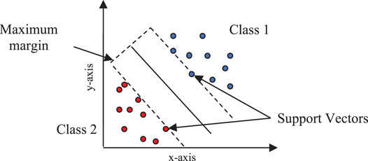
FIGURE 4. Binary support vector machine.
The authors considered a case of binary SVM as in Figure 4 (Chaudhary and Kumar, 2021). Suppose “
where w = weight vector (orthogonal to hyperplane), and b = bias (parameter that maintains the position of hyperplane at the maximum margin). The position of the hyperplane is determined by Eq. 23.
The class of the data points is determined by the following:
The SVM classifier was used for the LULC classification of the waterbody, urban, and vegetation using scattering components retrieved from different decomposition modeling approaches. The scattering response of the scatterers was used to train the SVM classifier. The radial bias function (RBF) was utilized for the classification. It requires less arithmetic calculative efforts and is capable of handling the nonlinear relationship between the input training pixels and the entire pixels of the datasets (Mishra et al., 2017a). The value of the RBF kernel is determined by the distance between the support vector point or the origin. Equation 24 represents the RBF kernel used by the SVM classifier (Chaudhary and Kumar, 2021).
where
The study area is comprised of various LULC features: 1) land use urban features such as residential colonies, road networks, bridges, high-rise buildings, oriented buildings, and industrial area; 2) very few vegetation cover structures such as forest, vegetation, and urban green space; and 3) a small portion of water bodies such as swimming pools, ponds, and sea surface. To achieve better accuracy in the classification of vegetation, urban, and waterbody, the SVM classifier requires the training sample pixels to represent all the different types of features for each class. So, the training sample was collected for each type of feature representing the individual classes. The size of the training sample for each class was different. The multifrequency and multi-temporal SAR datasets were used; the land cover may change from 2008 to 2017. Therefore, training pixel was collected carefully for each class for each sensor's datasets; the spatial resolution of each dataset was different, which caused variation in the training sample size collected for each dataset. The details of the training pixels used for the classification of Pauli, Barnes, Cloude, and Raney scattering components are given in Table 2.
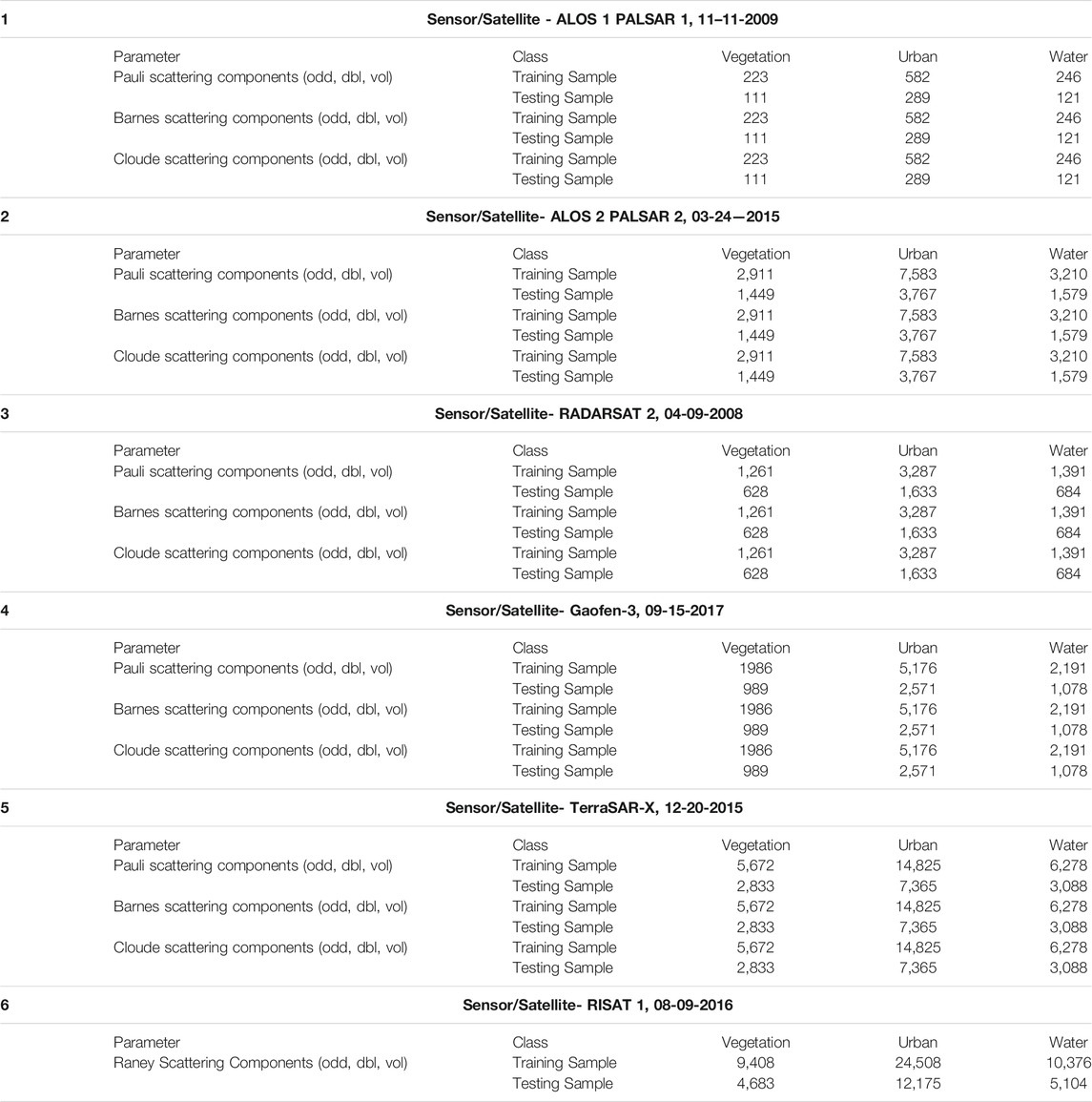
TABLE 2. Description of training sample and testing sample used for SVM classification of surface (odd), double-bounce (dbl), and volume (vol) scattering components retrieved from decomposition models using multi-temporal and multifrequency datasets.
Confusion Matrix and Accuracy Assessments
The accuracy of the LULC classification images was evaluated based on the error matrix approach (Lillesand and Kiefer, 1979; Congalton, 1991). It is the most effective method for analyzing classification accuracy. The error matrix, also referred to as the confusion matrix, compares the data (pixels) of each category/class of the classification result image with the ground reference data (pixels) to evaluate the accuracy. The error matrix provides descriptive measures such as overall accuracy (OA), user's accuracy (U.A), producer's accuracy (P.A), commission error, omission error, and kappa coefficient (
The KAPPA is a multivariate approach for the accuracy assessment, and its results are based on the KHAT statistics (
The ground reference data or testing sample for each class, i.e., vegetation, urban, and waterbody, was collected from the Google Earth platform. The historical optical images of Google Earth were coordinated to the date of acquisition of SAR datasets to collect the ground reference data. The sampling technique and size are important considerations for collecting the testing sample (Lillesand and Kiefer, 1979). The stratified random sampling technique was used to collect the testing samples, representing each land cover as strata. The study area consists of a variety of features. The testing samples were collected for all the features representing each class. The sample size of the testing pixels was half of the training pixels for each class. The description of the testing sample used for the accuracy assessment of each LULC image is shown in Table 2. The confusion matrix was produced to derive overall accuracy (O.A.) and kappa coefficient (
The presence of heterogeneous features in the study area and disproportionate LULC caused an imbalanced number of training pixels for individual classes. This study utilized multifrequency and multi-temporal SAR data of different sensors that caused imbalanced training sample sizes for each sensor's dataset (Table 2). The training sample size (the number of pixels) was significantly reduced for the low spatial resolution PolSAR datasets (i.e., ALOS-1 PALSAR-1) than for high spatial resolution datasets (i.e., TerraSAR-X, RISAT-1). The overall accuracy of the classification is influenced by the training sample size used by the classifier. However, several studies showed (Foody et al., 2006; Qian et al., 2015; Heydari and Mountrakis, 2018; Thanh Noi and Kappas, 2018) that the classification accuracy produced by the SVM classifier is least sensitive to the training sample size. The SVM creates the hyperplane or decision boundary based on support vectors instead of using all the training sample data. Therefore, the training sample size does not affect the SVM classification accuracy. A study by Qian et al. (2015) illustrated that the classification accuracy of the SVM classifier was significantly higher than the decision tree and k-nearest neighbor classifier, even for the small training sample data. Similarly, Thanh Noi and Kappas (2018) compared the effect of different training sample sizes for imbalanced and balanced training sample data using SVM, random forest, and k-nearest neighbor classifiers. They demonstrated that the imbalanced training sample data had the least impact on the SVM classifier's classification accuracy.
Result and Discussion
Comparison of Scattering Response for Vegetation, Urban, and Waterbody
The volume, double-bounce, and surface scattering responses retrieved from decomposition models were measured for the water, urban, and vegetation regions. The selected test area for the analysis is shown in Figures 1 and 3.
Vegetation
Figure 6 shows the scattering response for vegetation structure of decomposition models using multi-temporal and multifrequency datasets. The vegetation or forest canopy structure exhibited the volume scattering response due to multiple interactions with the branches, leaves, and tree trunks for the transmitted EM signals. The Pauli decomposition displayed the highest contribution to surface scattering response. The scattering components were coherent; therefore, it was suitable for the characterization of the homogeneous target within a single SAR resolution cell, hence failing to provide suitable scattering information. The Barnes decomposition displayed favorable results for the vegetation structure. The best volume scattering response was observed for L-band datasets due to its ability to penetrate the vegetation structure. However, the Cloude scattering components based on the eigenvalue–eigenvector approach failed to describe the appropriate scattering mechanism. It displayed a surface scattering response. The Raney decomposition model showed reliable information for vegetation structure. It displayed the highest contribution to volume scattering for CP datasets (Figure 5).
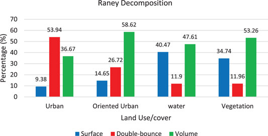
FIGURE 5. Scattering response for urban, oriented urban, and water (smooth) scatterer obtained from Raney decomposition.
The roll-invariant decomposition model was suitable for the study of vegetation structure (Figure 6B). The small contribution to surface scattering response in the vegetation region showed the interaction of emitted radar signal with the ground/smooth surface. Similarly, even-bounce scattering contribution illustrated the interaction between ground and tree trunks. From Figure 6, the volume scattering response associated with the vegetation cover was more intense for the longer wavelength (L-band). The intensity of volume scattering decreased for the shorter wavelength (X-band) because the penetration capacity of EM wave decreases with an increase in frequency. It shows that a low-frequency or longer wavelength dataset is more suitable for the study of vegetation or forest structures.
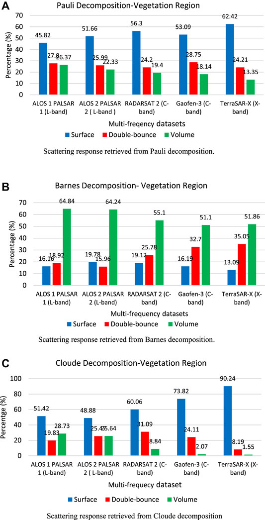
FIGURE 6. Scattering response for vegetation structure obtained from Pauli, Barnes, and Cloude decomposition models. (A) Scattering response retrieved from Pauli decomposition. (B) Scattering response retrieved from Barnes decomposition. (C) Scattering response retrieved from Cloude decomposition.
Urban Region
The urban structure is described as a dihedral structure that produces a double-bounce (even) scattering response for the incoming SAR sensor's EM radiations. In this study, the chosen test area for urban region consists of orthogonal urban structure and oriented urban structure; the scattering response was measured for both types of structures and shown in Figures 7 and 8.
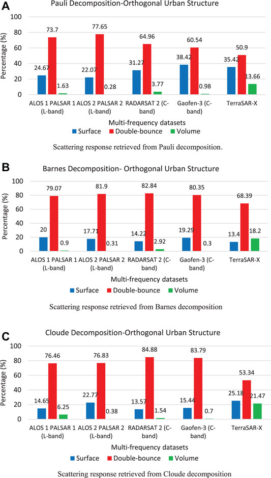
FIGURE 7. Backscattering response for orthogonal urban structure obtained from Pauli, Barnes, and Cloude decomposition models. (A) Scattering response retrieved from Pauli decomposition. (B) Scattering response retrieved from Barnes decomposition. (C) Scattering response retrieved from Cloude decomposition.
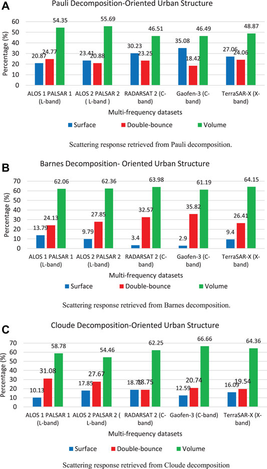
FIGURE 8. Backscattering response for oriented urban structure obtained from Pauli, Barnes, and Cloude decomposition models. (A) Scattering response retrieved from Pauli decomposition. (B) Scattering response retrieved from Barnes decomposition. (C) Scattering response retrieved from Cloude decomposition.
All the decomposition models provided reliable information for the orthogonal urban structure and illustrated the dominance of the double-bounce scattering response. The best double-bounce scattering response was obtained from Cloude and Barnes decomposition models using C-band datasets (RADARSAT-2, Gaofen-3). The Cloude and Barnes scattering components were roll-invariant, useful for characterizing the urban structure using C-band datasets. The Pauli scattering components were coherent, which was favorable for studying homogeneous structures. The Raney decomposition models showed a double-bounce scattering response for the CP RISAT-1 dataset.
For oriented urban structures, all the decomposition models overestimated volume scattering response and displayed the least contribution to double-bounce scattering response. From Figure 8, the Pauli decomposition displayed minimum contribution to the double-bounce scattering power. The Barnes decomposition improved the double-bounce scattering response to some extent, whereas Cloude decomposition reduced the volume scattering contribution. Similarly, the Raney decomposition model displayed volume scattering response for oriented urban structures (Figure 5). All the decomposition models failed to describe the appropriate scattering mechanism for oriented urban structure.
Water Region
The result of the scattering response retrieved from decomposition modeling approaches for water region is displayed in Figure 9. The water surface illustrates smooth or Bragg’s scatterer type, producing odd-bounce or surface scattering response for the transmitted EM wave. All the decomposition models described surface scattering response for water region using L-band and C-band datasets. The Raney decomposition displayed a higher contribution to volume scattering response than surface scattering response for waterbody (smooth surface) using CP datasets (Figure 5). The Cloude and Barnes displayed enhanced surface scattering response for ALOS-2 PALSAR-2 and Gaofen-3 due to an increase in spatial resolution of the datasets (Figure 9).
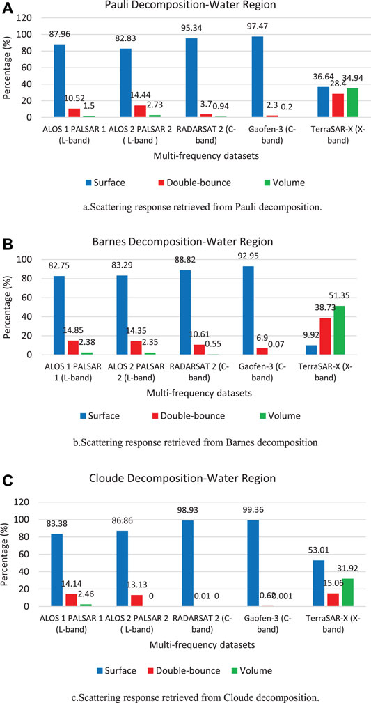
FIGURE 9. Backscattering response for water region obtained from Pauli, Barnes, and Cloude decomposition models.
All the decomposition models displayed the lowest surface scattering contribution for the waterbody using TerraSAR-X datasets. The Pauli and Barnes decomposition underestimated surface scattering mechanism and overestimated volume scattering response, whereas Cloude decomposition displayed surface scattering contribution. The low-frequency dataset provided very less scattering information for the characterization of smooth structures.
Comparison Land Use/Land Cover Classification of Scattering Components
Figure 10 represents the LULC images obtained from the classification of Pauli, Barnes, Cloude, and Raney scattering components (Figure 3), which were retrieved from the multifrequency PolSAR datasets, and Table 3 shows their accuracy assessment.
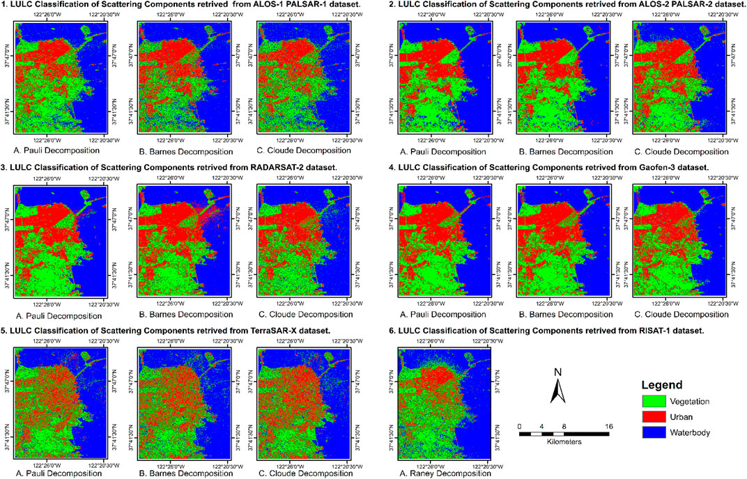
FIGURE 10. LULC images obtained from classification of Pauli, Barnes, Cloude scattering components extracted from multi-temporal and multifrequency datasets; Green—vegetation, Red—urban, and Blue—waterbody.
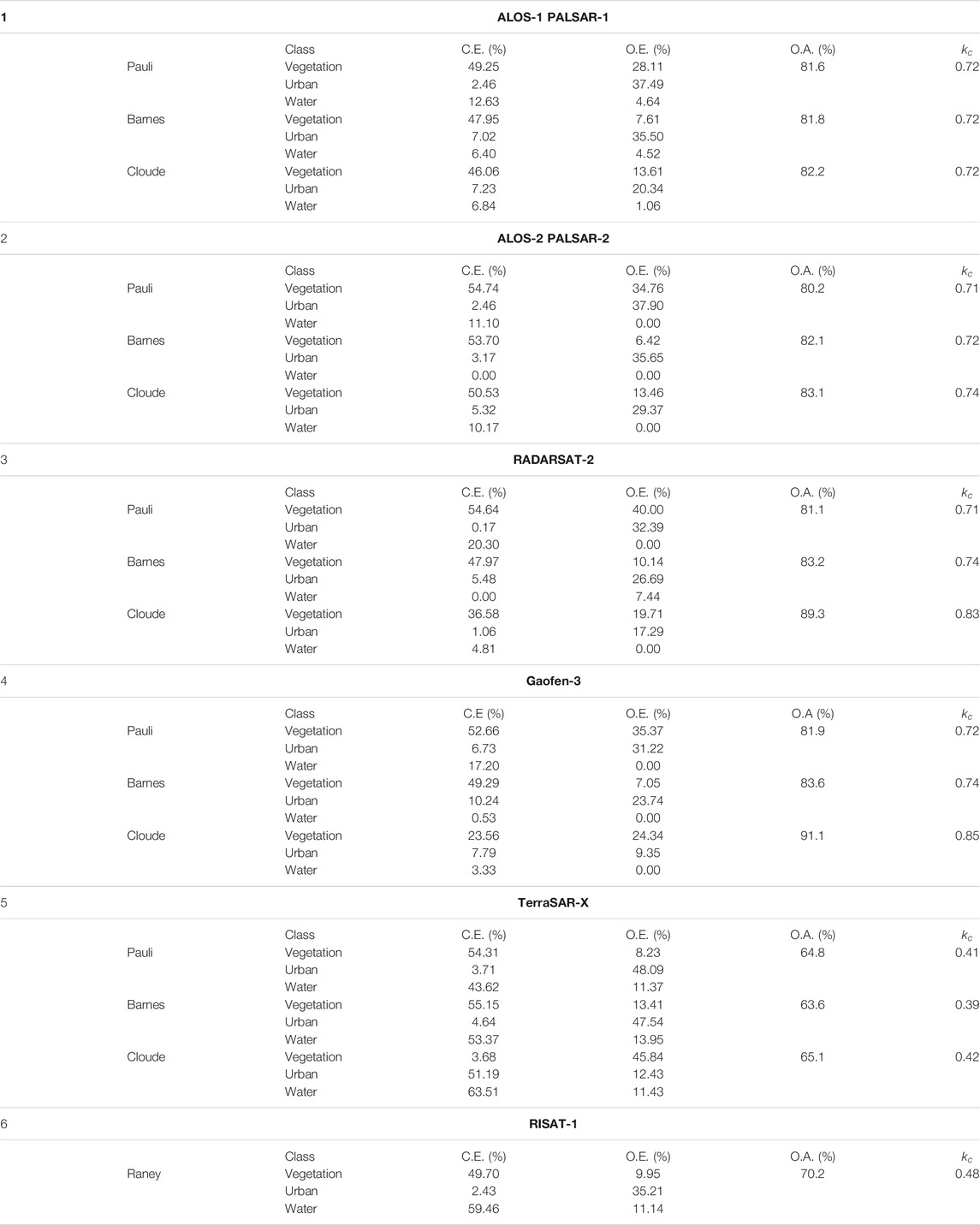
TABLE 3. Overall Accuracy (O.A), kappa coefficient (
Classification of Scattering Components Retrieved From L-Band ALOS-1 PALSAR-1 and ALOS-2 PALSAR-2 Datasets
The classification of the Pauli scattering component displayed O.A. values of 81.6% (
Classification of Scattering Components Retrieved From C-Band RADARSAT-2 and Gaofen-3 Datasets
The targets had demonstrated favorable scattering responses for C-band datasets. The Barnes and Cloude decomposition models displayed relatively good scattering responses to characterize dihedral (orthogonal) structures and smooth surfaces (waterbody) for C-band than the L-band datasets, which eventually increases the O.A. of the LULC classification. The Pauli decomposition displayed a relatively lower double-bounce scattering response for oriented urban structure for the C-band than the L-band datasets; therefore, it presented low accuracy in the classification. The classification of coherent scattering component of Pauli decomposition displayed O.A. values of 81.1% (
Classification of Scattering Components Retrieved From TerraSAR-X Dataset
As shown in Table 3, the classification of Pauli scattering components presented an O.A. of 64.8% (
The Pauli,Barnes, and Cloude decomposition models demonstrated the least reliable scattering information to identify the target for TerraSAR-X datasets. Eventually, the classification of scattering components presented the least overall accuracy in the classification. The Pauli decomposition displayed an underestimation of the volume scattering mechanism for vegetation structure. The Barnes decomposition underestimated surface scattering response for the water region. The Cloude decomposition misinterpreted the vegetation structure as a smooth scatterer. Therefore, the error was highest for each class (Table 3) due to the misinterpretation of the targets.
Classification of Scattering Components Retrieved From Compact-Pol RISAT-1 Dataset
The Raney decomposition model showed suitable scattering information about the orthogonal urban structure and vegetation region. However, it underestimated the surface scattering mechanism for the smooth scatterer (waterbody) and double-bounce scattering response for oriented urban structures. Hence, the accuracy of water and the urban class was low due to misinterpretation of the target. The Raney scattering components presented an O.A. of 70.2% (
The coherent decomposition models are suitable for the study of “pure targets” or homogeneous targets within a single resolution cell, and incoherent decomposition models are favorable for the study of “distributed targets” or heterogeneous targets. The classification of Cloude and Barnes scattering components showed higher O.A. than Pauli scattering components (Figure 11). All the decomposition models overestimated the volume scattering mechanism for oriented urban structure, which led to the misclassification of the urban pixels into vegetation class. Therefore, the omission error was highest for the urban class, and the commission error was highest for the vegetation class in the output LULC images. The water class presented the lowest error in the classification because all the decomposition models appropriately described the surface scattering mechanism for the waterbody (Table 3).
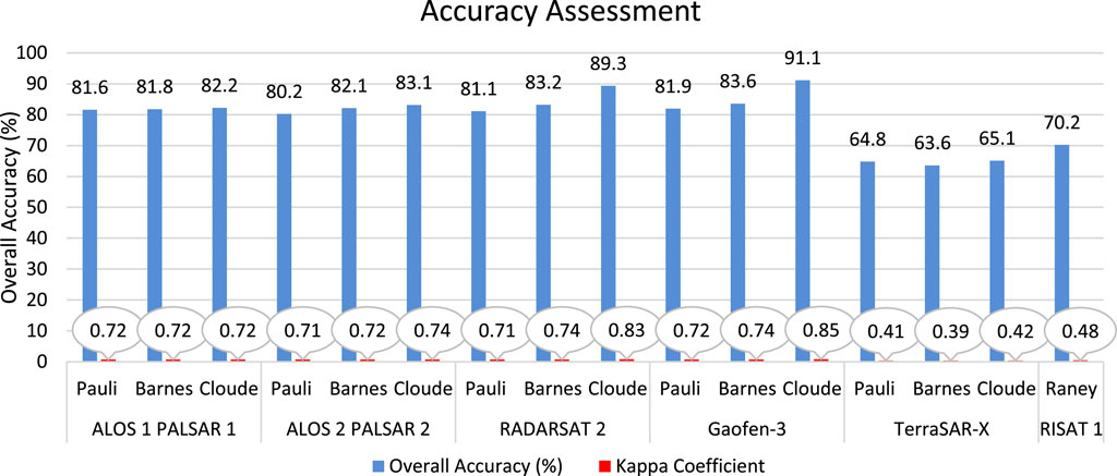
FIGURE 11. Overall accuracy, kappa coefficient (
The roll-invariant Barnes and Cloude decomposition models demonstrated a relatively better double-bounce scattering mechanism for orthogonal structure using C-band datasets than L-band (Figures 7B,C). Therefore, the C-band dataset displayed higher accuracy for the urban class than the L-band datasets (Figure 12A) in the classification. The roll-invariant Barnes decomposition provided desirable scattering information for the characterization of vegetation structure using C-band datasets (Figure 6B), presenting good accuracy for the classification of the vegetation class (Figure 12B).
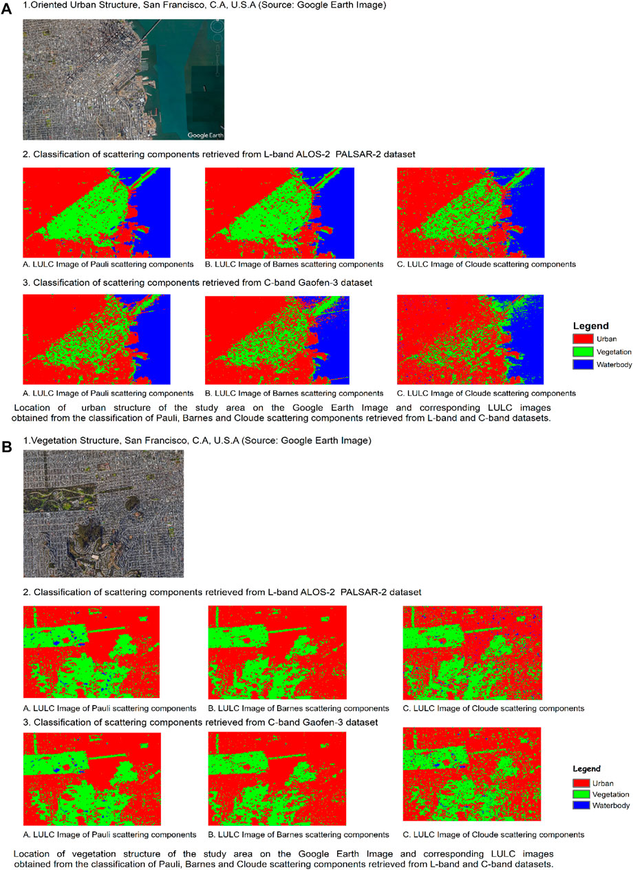
FIGURE 12. Location of vegetation structure and urban structure of study area on Google Earth Image and corresponding LULC images obtained from classification of Pauli, Barnes, and Cloude scattering components retrieved from L-band and C-band datasets.
Conclusion
The main objective of this study was to use multifrequency spaceborne SAR data that were acquired over San Francisco City from the years 2008–2017. This study explored and compared the classification outputs of multifrequency spaceborne PolSAR data. The classification schemes were performed for scattering-based characterization of LULC using multifrequency SAR sensor's ALOS-1 PALSAR-1, ALOS-2 PALSAR-2, RADARSAT-2, Gaofen-3, TerraSAR-X, and RISAT-1 dataset. The coherent-based Pauli decomposition model demonstrated reliable scattering information for “pure target” within a single cell such as a homogeneous waterbody and orthogonal urban structures. The roll-invariant Barnes decomposition provided fruitful scattering information for vegetation and urban structure. The eigenvalue–eigenvector-based Cloude decomposition model described a favorable scattering mechanism for the characterization of urban and waterbody. These decomposition modeling approaches failed to provide reliable scattering information to characterize oriented urban structures. The CP Raney decomposition provided desirable scattering information for vegetation and orthogonal urban structure. The classification of Raney scattering components presented 70.2% (
Data Availability Statement
The original contributions presented in the study are included in the article/Supplementary Material, further inquiries can be directed to the corresponding author.
Author Contributions
Writing—original draft preparation, SV; conceptualization, SK and SV; satellite data acquisition, SK; software, SK; methodology, SK; writing—review and editing, SV, SK, VM, and RR; supervision of the project, SK and VM; visualization SV, SK, VM, and RR.
Conflict of Interest
The authors declare that the research was conducted in the absence of any commercial or financial relationships that could be construed as a potential conflict of interest.
Publisher’s Note
All claims expressed in this article are solely those of the authors and do not necessarily represent those of their affiliated organizations or those of the publisher, the editors, and the reviewers. Any product that may be evaluated in this article, or claim that may be made by its manufacturer, is not guaranteed or endorsed by the publisher.
Acknowledgments
The authors are thankful to the German Aerospace Center (DLR) Oberpfaffenhofen for providing TerraSAR-X data to SK under the Project Id -NTI_POLI6635 on PolInSAR Tomography for above ground biomass estimation. The authors would like to express their sincere gratitude to the whole research team of ESA for providing SNAP 8.0 and the Polarimetric SAR data Processing and Educational Toolbox PolSARPro 6.0.3 (Biomass Edition) tools for polarimetric processing of the SAR data. The authors are grateful to the Institute of Electronics and Telecommunications of Rennes (IETR), Rennes, France, for maintaining the portal to download the PolSAR data (RISAT-1, ALOS-1 PALSAR-1, ALOS-2 PALSAR-2, GAOFEN-3, and RADARSAT-2) for San Francisco City and the software/tool PolSARPro 6.0.3.
References
Agrawal, N., Kumar, S., and Tolpekin, V. (2016). Polarimetric SAR Interferometry-Based Decomposition Modelling for Reliable Scattering Retrieval. SPIE Proceedings,Land Surf. Cryosphere Remote Sensing. 9877, 31–40. doi:10.1117/12.2223977
Alberga, V. (2007). A Study of Land Cover Classification Using Polarimetric SAR Parameters. Int. J. Remote Sensing. 28, 3851–3870. doi:10.1080/01431160601075541
Ali, Z., Kroupnik, G., Matharu, G., Graham, J., Barnard, I., Fox, P., et al. (2014). RADARSAT-2 Space Segment Design and its Enhanced Capabilities with Respect to RADARSAT-1. Can. J. Remote Sensing. 30, 235–245. doi:10.5589/M03-077
ArcGIS Desktop | Download and Documentation (2022). Available at: https://www.esri.com/en-us/arcgis/products/arcgis-desktop/resources (Accessed January 3, 2022).
Awasthi, S., Thakur, P. K., Kumar, S., Kumar, A., Jain, K., and Mani, S. (2020). Snow Density Retrieval Using Hybrid Polarimetric RISAT-1 Datasets. IEEE J. Sel. Top. Appl. Earth Obs. Remote Sens. 13, 3058–3065. doi:10.1109/JSTARS.2020.2991156
Babu, A., Kumar, S., and Agrawal, S. (2021a). Polarimetric Calibration and Spatio‐temporal Polarimetric Distortion Analysis of UAVSAR PolSAR Data. Earth Space Sci. 8, e2020EA001629. doi:10.1029/2020EA001629
Babu, A., Kumar, S., and Agrawal, S. (2021b). Polarimetric Calibration of L-Band UAVSAR Data. J. Indian Soc. Remote Sens. 49, 541–549. doi:10.1007/s12524-020-01241-1
Babu, A., Kumar, S., and Agrawal, S. (2019a). Polarimetric Calibration of RISAT-1 Compact-Pol Data. IEEE J. Sel. Top. Appl. Earth Observations Remote Sensing. 12, 3731–3736. doi:10.1109/jstars.2019.2932019
Babu, A., Kumar, S., and Agrawal, S. (2019b). RISAT-1 Compact Polarimetric Calibration and Decomposition. Proceedings. 18, 3. doi:10.3390/ECRS-3-06189
Bai, Y., Sun, G., Li, Y., Ma, P., Li, G., and Zhang, Y. (2021). Comprehensively Analyzing Optical and Polarimetric SAR Features for Land-Use/land-Cover Classification and Urban Vegetation Extraction in Highly-Dense Urban Area. Int. J. Appl. Earth Observation Geoinformation. 103, 102496. doi:10.1016/j.jag.2021.102496
Bhanu Prakash, M., and Kumar, S. (2021a). Multifrequency Analysis of PolInSAR-Based Decomposition Using Cosine-Squared Distribution. IETE Tech. Rev. 0, 1–8. doi:10.1080/02564602.2021.1892542
Bhanu Prakash, M., and Kumar, S. (2021b). PolInSAR Decorrelation-Based Decomposition Modelling of Spaceborne Multifrequency SAR Data. Int. J. Remote Sensing. 42, 1398–1419. doi:10.1080/01431161.2020.1829155
Bhattacharya, A., Muhuri, A., De, S., Manickam, S., and Frery, A. C. (2015). Modifying the Yamaguchi Four-Component Decomposition Scattering Powers Using a Stochastic Distance. IEEE J. Sel. Top. Appl. Earth Observations Remote Sensing. 8, 3497–3506. doi:10.1109/jstars.2015.2420683
Bole, A., Wall, A., and Norris, A. (2014). “Chapter 3-Target Detection,” in Radar and ARPA Manual. Editors A. Bole, A. Wall, and A. Norris. Third Edition (Oxford: Butterworth-Heinemann), 139–213. doi:10.1016/B978-0-08-097752-2.00003-9
Boser, B. E., Guyon, I. M., and Vapnik, V. N. (1992). “Training Algorithm for Optimal Margin Classifiers,” in Proceedings of the Fifth Annual ACM Workshop on Computational Learning Theory COLT ’92 (New York, NY: Association for Computing Machinery), 144–152. doi:10.1145/130385.130401
Brusch, S., Lehner, S., Fritz, T., Soccorsi, M., Soloviev, A., and van Schie, B. (2011). Ship Surveillance with TerraSAR-X. IEEE Trans. Geosci. Remote Sensing. 49, 1092–1103. doi:10.1109/tgrs.2010.2071879
Buono, A., Nunziata, F., Migliaccio, M., Yang, X., and Li, X. (2017). Classification of the Yellow River delta Area Using Fully Polarimetric SAR Measurements. Int. J. Remote Sensing. 38, 6714–6734. doi:10.1080/01431161.2017.1363437
Chaudhary, V., and Kumar, S. (2021). Dark Spot Detection for Characterization of marine Surface Slicks Using UAVSAR Quad-Pol Data. Sci. Rep. 11, 8975. doi:10.1038/s41598-021-88301-9
Chaudhary, V., and Kumar, S. (2020). Marine Oil Slicks Detection Using Spaceborne and Airborne SAR Data. Adv. Space Res. 66, 854–872. doi:10.1016/j.asr.2020.05.003
Chaussard, E., Amelung, F., Abidin, H., and Hong, S.-H. (2013). Sinking Cities in Indonesia: ALOS PALSAR Detects Rapid Subsidence Due to Groundwater and Gas Extraction. Remote Sensing Environ. 128, 150–161. doi:10.1016/j.rse.2012.10.015
Chen, S.-W., Li, Y.-Z., Wang, X.-S., Xiao, S.-P., and Sato, M. (2014a). Modeling and Interpretation of Scattering Mechanisms in Polarimetric Synthetic Aperture Radar: Advances and Perspectives. IEEE Signal. Process. Mag. 31, 79–89. doi:10.1109/msp.2014.2312099
Chen, S. W., Xue-Song Wang, X. S., Yong-Zhen Li, Y. Z., and Sato, M. (2014b). Adaptive Model-Based Polarimetric Decomposition Using Polinsar Coherence. IEEE Trans. Geosci. Remote Sensing. 52, 1705–1718. doi:10.1109/tgrs.2013.2253780
Chen, S.-W., and Sato, M. (2013). Tsunami Damage Investigation of Built-Up Areas Using Multitemporal Spaceborne Full Polarimetric SAR Images. IEEE Trans. Geosci. Remote Sensing. 51, 1985–1997. doi:10.1109/tgrs.2012.2210050
Chen, S.-W., Wang, X.-S., Xiao, S.-P., and Sato, M. (2018). “Fundamentals of Polarimetric Radar Imaging and Interpretation,” in Target Scattering Mechanism in Polarimetric Synthetic Aperture Radar: Interpretation and Application (Singapore: Springer Singapore), 1–42. doi:10.1007/978-981-10-7269-7_1
Cloude, S. R., Goodenough, D. G., and Chen, H. (2012). Compact Decomposition Theory. IEEE Geosci. Remote Sensing Lett. 9, 28–32. doi:10.1109/lgrs.2011.2158983
Cloude, S. R. (1985). Target Decomposition Theorems in Radar Scattering. Electronics Lett. 21, 22–24. doi:10.1049/el:19850018
Congalton, R. G. (1991). A Review of Assessing the Accuracy of Classifications of Remotely Sensed Data. Remote Sensing Environ. 37, 35–46. doi:10.1016/0034-4257(91)90048-B
ENVI® | Image Processing & Analysis Software (2022). Available at: https://www.l3harrisgeospatial.com/Software-Technology/ENVI (Accessed January 3, 2022).
Ferro-Famil, L., and Pottier, E. (2016). “1 - Synthetic Aperture Radar Imaging,” in Microwave Remote Sensing of Land Surface. Editors N. Baghdadi, and M. Zribi (Oxford: Elsevier), 1–65. doi:10.1016/B978-1-78548-159-8.50001-3
Foody, G. M., Mathur, A., Sanchez-Hernandez, C., and Boyd, D. S. (2006). Training Set Size Requirements for the Classification of a Specific Class. Remote Sensing Environ. 104, 1–14. doi:10.1016/j.rse.2006.03.004
Freeman, A., and Durden, S. L. (1998). A Three-Component Scattering Model for Polarimetric SAR Data. IEEE Trans. Geosci. Remote Sensing 36, 963–973. doi:10.1109/36.673687
Freeman, A. (2007). Fitting a Two-Component Scattering Model to Polarimetric SAR Data from Forests. IEEE Trans. Geosci. Remote Sensing. 45, 2583–2592. doi:10.1109/tgrs.2007.897929
Garg, R., Kumar, A., Prateek, M., Pandey, K., and Kumar, S. (2022). Land Cover Classification of Spaceborne Multifrequency SAR and Optical Multispectral Data using Machine Learning. Adv. Space Res. 69, 1726–1742. doi:10.1016/j.asr.2021.06.028
Heydari, S. S., and Mountrakis, G. (2018). Effect of Classifier Selection, Reference Sample Size, Reference Class Distribution and Scene Heterogeneity in Per-Pixel Classification Accuracy Using 26 Landsat Sites. Remote Sensing Environ. 204, 648–658. doi:10.1016/j.rse.2017.09.035
Holm, W. A., and Barnes, R. M. (1988). “On Radar Polarization Mixed Target State Decomposition Techniques,” in Decomposition Techniques (IEEE), 249–254. doi:10.1109/nrc.1988.10967
Huynen, J. R. (1978). “Phenomenological Theory of Radar Targets,” in Electromagnetic Scattering. Editor P. L. E. Uslenghi (New York: Academic Press), 653–712. doi:10.1016/B978-0-12-709650-6.50020-1
Jafari, M., Maghsoudi, Y., and Valadan Zoej, M. J. (2015). A New Method for Land Cover Characterization and Classification of Polarimetric SAR Data Using Polarimetric Signatures. IEEE J. Sel. Top. Appl. Earth Observations Remote Sensing. 8, 3595–3607. doi:10.1109/jstars.2014.2387374
Jordan, R. (1980). The Seasat-A Synthetic Aperture Radar System. IEEE J. Oceanic Eng. 5, 154–164. doi:10.1109/joe.1980.1145451
Kranjčić, N., Medak, D., Župan, R., and Rezo, M. (2019). Machine Learning Methods for Classification of the Green Infrastructure in City Areas. Ijgi. 8 (8), 463. doi:10.3390/IJGI8100463
Krogager, E. (1990). New Decomposition of the Radar Target Scattering Matrix. Electron. Lett. 26, 1525. doi:10.1049/el:19900979
Kumar, P., Gupta, D. K., Mishra, V. N., and Prasad, R. (2015). Comparison of Support Vector Machine, Artificial Neural Network, and Spectral Angle Mapper Algorithms for Crop Classification Using LISS IV Data. Int. J. Remote Sensing 36, 1604–1617. doi:10.1080/2150704X.2015.1019015
Kumar, S., Babu, A., Agrawal, S., Asopa, U., Shukla, S., and Maiti, A. (2022). Polarimetric Calibration of Spaceborne and Airborne Multifrequency SAR Data for Scattering-Based Characterization of Manmade and Natural Features. Adv. Space Res. 69, 1684–1714. doi:10.1016/j.asr.2021.02.023
Kumar, S., Garg, R. D., Govil, H., and Kushwaha, S. P. S. (2019). PolSAR-Decomposition-Based Extended Water Cloud Modeling for Forest Aboveground Biomass Estimation. Remote Sensing 11 (11), 2287. doi:10.3390/RS11192287
Kumar, S., Govil, H., Srivastava, P. K., Thakur, P. K., and Kushwaha, S. P. S. (2020). Spaceborne Multifrequency PolInSAR-Based Inversion Modelling for Forest Height Retrieval. Remote Sensing 12 (12), 4042. doi:10.3390/RS12244042
Lardeux, C., Frison, P.-L., Tison, C., Souyris, J.-C., Stoll, B., Fruneau, B., et al. (2009). Support Vector Machine for Multifrequency SAR Polarimetric Data Classification. IEEE Trans. Geosci. Remote Sensing 47, 4143–4152. doi:10.1109/tgrs.2009.2023908
Lee, J.-S., and Pottier, E. (2009). Polarimetric Radar Imaging From Basics to Applications. 1st Edn. Boca Raton: CRC Press, Taylor & Fancis Group. doi:10.1201/9781420054989
Lillesand, T. M., and Kiefer, R. W. (1979). Remote Sensing and Image Interpretation. 1st Edn. New York: John Wiley & Sons, Ltd.
Lu, D. (2007). A Survey of Image Classification Methods and Techniques for Improving Classification Performance. Int. J. Remote Sensing 28, 823–870. doi:10.1080/01431160600746456
Maghsoudi, Y. (2011). Analysis of Radarsat-2 Full Polarimetric Data for Forest Mapping. Dep. Geomatics Eng. Univ. Calgary. Degree PhD.
Mahmood, A. (1997). RADARSAT-1 Background Mission for a Global SAR Coverage. Igarss’97. 1997 IEEE Int. Geosci. Remote Sensing Symp. Proc. Remote Sensing - A Scientific Vis. Sustainable Development Vol. 3, 1217. doi:10.1109/IGARSS.1997.606402
Maiti, A., Kumar, S., Tolpekin, V., and Agarwal, S. (2021). A Computationally Efficient Hybrid Framework for Polarimetric Calibration of Quad‐Pol SAR Data. Earth Space Sci. 8, e2020EA001447. doi:10.1029/2020EA001447
Mason, D. C., Speck, R., Devereux, B., Schumann, G. J.-P., Neal, J. C., and Bates, P. D. (2010). Flood Detection in Urban Areas Using TerraSAR-X. IEEE Trans. Geosci. Remote Sensing 48, 882–894. doi:10.1109/tgrs.2009.2029236
Mishra, V. N., Prasad, R., Kumar, P., Gupta, D. K., and Srivastava, P. K. (2017a). Dual-polarimetric C-Band SAR Data for Land Use/land Cover Classification by Incorporating Textural Information. Environ. Earth Sci. 76, 1. doi:10.1007/S12665-016-6341-7
Mishra, V. N., Prasad, R., Kumar, P., Srivastava, P. K., and Rai, P. K. (2017b). Knowledge-based Decision Tree Approach for Mapping Spatial Distribution of rice Crop Using C-Band Synthetic Aperture Radar-Derived Information. J. Appl. Remote Sens. 11, 1. doi:10.1117/1.JRS.11.046003
Mishra, V. N., Prasad, R., Rai, P. K., Vishwakarma, A. K., and Arora, A. (2019). Performance Evaluation of Textural Features in Improving Land Use/land Cover Classification Accuracy of Heterogeneous Landscape Using Multi-Sensor Remote Sensing Data. Earth Sci. Inform. 12, 71–86. doi:10.1007/S12145-018-0369-Z
Misra, T., and Kirankumar, A. S. (2014). “RISAT-1: Configuration and Performance Evaluation,” in 2014 XXXIth URSI General Assembly and Scientific Symposium (URSI GASS) (Beijing: IEEE), 1–4. doi:10.1109/URSIGASS.2014.6929612
Misra, T., Rana, S. S., Desai, N. M., Dave, D. B., Rajeevjyoti, , Arora, R. K., et al. (2013). Synthetic Aperture Radar Payload On-Board RISAT-1: Configuration, Technology and Performance. Curr. Sci. 104, 446–461. Available at: https://www.currentscience.ac.in/Volumes/104/04/0446.pdf.
Morena, L. C., James, K. V., and Beck, J. (2004). V, and Beck, JAn Introduction to the RADARSAT-2 mission. Can. J. Remote Sensing 30, 221–234. doi:10.5589/m04-004
Ng, A. H.-M., Ge, L., Li, X., Abidin, H. Z., Andreas, H., and Zhang, K. (2012). Mapping Land Subsidence in Jakarta, Indonesia Using Persistent Scatterer Interferometry (PSI) Technique with ALOS PALSAR. Int. J. Appl. Earth Observation Geoinformation 18, 232–242. doi:10.1016/j.jag.2012.01.018
Niu, X., and Ban, Y. (2013). Multi-temporal RADARSAT-2 Polarimetric SAR Data for Urban Land-Cover Classification Using an Object-Based Support Vector Machine and a Rule-Based Approach. Int. J. Remote Sensing 34, 1–26. doi:10.1080/01431161.2012.700133
Orieschnig, C. A., Belaud, G., Venot, J.-P., Massuel, S., and Ogilvie, A. (2021). Input Imagery, Classifiers, and Cloud Computing: Insights from Multi-Temporal LULC Mapping in the Cambodian Mekong Delta. Eur. J. Remote Sensing 54, 398–416. doi:10.1080/22797254.2021.1948356
Pal, M., and Foody, G. M. (2010). Feature Selection for Classification of Hyperspectral Data by SVM. IEEE Trans. Geosci. Remote Sensing 48, 2297–2307. doi:10.1109/tgrs.2009.2039484
PolSARpro v6.0 (Biomass Edition) Toolbox Download – STEP (2022). Available at: https://step.esa.int/main/download/polsarpro-v6-0-biomass-edition-toolbox-download/(Accessed January 3, 2022).
Qi, Z., Yeh, A. G.-O., Li, X., and Lin, Z. (2012). A Novel Algorithm for Land Use and Land Cover Classification Using RADARSAT-2 Polarimetric SAR Data. Remote Sensing Environ. 118, 21–39. doi:10.1016/j.rse.2011.11.001
Qian, Y., Zhou, W., Yan, J., Li, W., and Han, L. (2015). Comparing Machine Learning Classifiers for Object-Based Land Cover Classification Using Very High Resolution Imagery. Remote Sensing 7, 153–168. doi:10.3390/rs70100153
Raney, R. K., Cahill, J. T. S., Patterson, G. W., and Bussey, D. B. J. (2012). Them-chidecomposition of Hybrid Dual-Polarimetric Radar Data with Application to Lunar Craters. J. Geophys. Res. 117, a–n. doi:10.1029/2011JE003986
Rawat, A., Kumar, A., Upadhyay, P., and Kumar, S. (2021). Deep Learning-Based Models for Temporal Satellite Data Processing: Classification of Paddy Transplanted fields. Ecol. Inform. 61, 101214. doi:10.1016/j.ecoinf.2021.101214
Rosen, P. A., Kim, Y., Kumar, R., Misra, T., Bhan, R., and Sagi, V. R. (2017). Global Persistent SAR Sampling with the NASA-ISRO SAR (NISAR) mission. 2017 IEEE Radar Conf. RadarConf 2017, 0410–0414. doi:10.1109/radar.2017.7944237
Rosenqvist, A., Shimada, M., Ito, N., and Watanabe, M. (2007). ALOS PALSAR: A Pathfinder mission for Global-Scale Monitoring of the Environment. IEEE Trans. Geosci. Remote Sensing 45, 3307–3316. doi:10.1109/tgrs.2007.901027
Rosenqvist, A., Shimada, M., Suzuki, S., Ohgushi, F., Tadono, T., Watanabe, M., et al. (2014). Operational Performance of the ALOS Global Systematic Acquisition Strategy and Observation Plans for ALOS-2 PALSAR-2. Remote Sensing Environ. 155, 3–12. doi:10.1016/j.rse.2014.04.011
Saito, N., Yamada, H., and Yamaguchi, Y. (2018). “Study on Land Classification of PolSAR Data by Using Support Vector Machine,” in 2018 IEEE International Workshop on Electromagnetics:Applications and Student Innovation Competition (iWEM). doi:10.1109/iWEM.2018.8536619
Sato, M., Chen, S. W., and Satake, M. (2012). Polarimetric SAR Analysis of Tsunami Damage Following the March 11, 2011 East Japan Earthquake. Proc. IEEE 100, 2861–2875. doi:10.1109/JPROC.2012.2200649
Scheuchl, B., Flett, D., Caves, R., and Cumming, I. (2014). Potential of RADARSAT-2 Data for Operational Sea Ice Monitoring. Can. J. Remote Sensing 30, 448–461. doi:10.5589/M04-011
Schuler, D., Lee, J. S., Kasilingam, D., and Pottier, E. (2004). Measurement of Ocean Surface Slopes and Wave Spectra Using Polarimetric SAR Image Data. Remote Sensing Environ. 91, 198–211. doi:10.1016/j.rse.2004.03.008
Schuler, D. L., Jansen, R. W., Lee, J. S., and Kasilingam, D. (2003). Polarisation Orientation Angle Measurements of Ocean Internal Waves and Current Fronts Using Polarimetric SAR. IEE Proc. Radar Sonar Navig. 150, 135. doi:10.1049/ip-rsn:20030492
Shafai, S. S., and Kumar, S. (2020). PolInSAR Coherence and Entropy‐Based Hybrid Decomposition Model. Earth Space Sci. 7, e2020EA001279. doi:10.1029/2020EA001279
Singh, G., and Yamaguchi, Y. (2018). Model-Based Six-Component Scattering Matrix Power Decomposition. IEEE Trans. Geosci. Remote Sensing 56, 5687–5704. doi:10.1109/tgrs.2018.2824322
SNAP 8.0 released – STEP (2022). Available at: https://step.esa.int/main/snap-8-0-released/(Accessed January 3, 2022).
Stewart, C., Lasaponara, R., and Schiavon, G. (2013). ALOS PALSAR Analysis of the Archaeological Site of Pelusium. Archaeol. Prospect. 20, 109–116. doi:10.1002/ARP.1447
Thanh Noi, P., and Kappas, M. (2018). Comparison of Random Forest, K-Nearest Neighbor, and Support Vector Machine Classifiers for Land Cover Classification Using Sentinel-2 Imagery. Sensors 18, 18. doi:10.3390/s18010018
Tomar, K. S., Kumar, S., and Tolpekin, V. A. (2019). Evaluation of Hybrid Polarimetric Decomposition Techniques for Forest Biomass Estimation. IEEE J. Sel. Top. Appl. Earth Observations Remote Sensing 12, 3712–3718. doi:10.1109/jstars.2019.2947088
van Zyl, J. J. (1993). “Application of Cloude's Target Decomposition Theorem to Polarimetric Imaging Radar Data,” in Radar Polarimetry. Editors H. Mott, and W.-M. Boerner (San Diego: SPIE), 184–191. doi:10.1117/12.140615
Vapnik, V. N. (1995). “Introduction: Four Periods in the Research of the Learning Problem,” in The Nature of Statistical Learning Theory (New York, NY: Springer New York), 1–14. doi:10.1007/978-1-4757-2440-0_1
Velotto, D., Migliaccio, M., Nunziata, F., and Lehner, S. (2011). Dual-polarized Terrasar-X Data for Oil-Spill Observation. IEEE Trans. Geosci. Remote Sensing 49, 4751–4762. doi:10.1109/tgrs.2011.2162960
Werninghaus, R., and Buckreuss, S. (2010). The TerraSAR-X mission and System Design. IEEE Trans. Geosci. Remote Sensing 48, 606–614. doi:10.1109/tgrs.2009.2031062
Yamaguchi, Y., Moriyama, T., Ishido, M., and Yamada, H. (2005). Four-component Scattering Model for Polarimetric SAR Image Decomposition. IEEE Trans. Geosci. Remote Sensing 43, 1699–1706. doi:10.1109/tgrs.2005.852084
Yamaguchi, Y., Yajima, Y., and Yamada, H. (2006). A Four-Component Decomposition of POLSAR Images Based on the Coherency Matrix. IEEE Geosci. Remote Sensing Lett. 3, 292–296. doi:10.1109/lgrs.2006.869986
Yin, Q., Cheng, J., Zhang, F., Zhou, Y., Shao, L., and Hong, W. (2020). Interpretable POLSAR Image Classification Based on Adaptive-Dimension Feature Space Decision Tree. IEEE Access 8, 173826–173837. doi:10.1109/access.2020.3023134
Yin, Q., Hong, W., Zhang, F., and Pottier, E. (2018). “Analysis of Polarimetric Feature Combination Based on Polsar Image Classification Performance with Machine Learning Approach,” in IGARSS 2018-2018 IEEE International Geoscience and Remote Sensing Symposium. doi:10.1109/IGARSS.2018.8517585
Keywords: multifrequency spaceborne SAR, eigenvalue-eigenvector, roll-invariant, compact-polarimetric decomposition, support vector machine, land use and land cover classification
Citation: Verma S, Kumar S, Mishra VN and Raj R (2022) Multifrequency Spaceborne Synthetic Aperture Radar Data for Backscatter-Based Characterization of Land Use and Land Cover. Front. Earth Sci. 10:825255. doi: 10.3389/feart.2022.825255
Received: 30 November 2021; Accepted: 14 February 2022;
Published: 24 March 2022.
Edited by:
Christian Bignami, Istituto Nazionale di Geofisica e Vulcanologia (INGV), ItalyReviewed by:
Milad Janalipour, K. N. Toosi University of Technology, IranMukesh Gupta, Catholic University of Louvain, Belgium
Copyright © 2022 Verma, Kumar, Mishra and Raj. This is an open-access article distributed under the terms of the Creative Commons Attribution License (CC BY). The use, distribution or reproduction in other forums is permitted, provided the original author(s) and the copyright owner(s) are credited and that the original publication in this journal is cited, in accordance with accepted academic practice. No use, distribution or reproduction is permitted which does not comply with these terms.
*Correspondence: Shashi Kumar, c2hhc2hpQGlpcnMuZ292Lmlu