 Rasheed Ajala
 Patricia Persaud
 Alan Juarez2
- 1Department of Geology and Geophysics, Louisiana State University, Baton Rouge, LA, United States
- 2Department of Earth Sciences, University of Southern CA, Los Angeles, CA, United States
Accurately predicting the seismic wavefield is important for physics-based earthquake hazard studies and is dependent on an accurate source model, a good model of the subsurface geology, and the full physics of wave propagation. Here, we conduct numerical experiments to investigate the effect of different representations of the Southern California Earthquake Center and Harvard community velocity models on seismic waveform predictions in the vicinity of the San Andreas fault in Salton Trough. We test general preconceptions about the importance of topography, near-surface geotechnical layering, and anelastic attenuation up to a maximum frequency of 0.5 Hz. For the Southern California Earthquake Center model developed without topography, we implement 1D and linear model extensions that preserve the geologic structure and a pull-up approach that adapts the original model to topographic variations and distorts the subsurface. The Harvard model includes an elevation model, so we test the squashed topography representation, which flattens it. For both community models, we modify the top 350 m by partially applying the Ely geotechnical layer using a minimum shear wave velocity of 600 m/s and incorporate an Olsen attenuation model using a ratio of 0.05. We evaluate the resulting 24 model representations using the classical waveform misfit and five moderate-magnitude earthquakes. Only the inclusion of attenuation consistently improves the wavefield predictions. It becomes more impactful at higher frequencies, where it significantly improves the performance levels of the crude 1D and linear extension models close to that of the original version. The pull-up topography representation also enhances the waveform prediction ability of the original model. Squashing the topography of the elevation-referenced Harvard model produces better seismogram fits, suggesting that seismic imagers construct community tomographic models without topography to avoid issues related to missing model parameters near the free surface or discrepancies with a different elevation model. Although full implementation of the Ely geotechnical layer that would permit shear wave velocities as low as 90 m/s proves computationally expensive, our partial implementation provides slightly better results in some cases. Our results can serve as recommendations for implementing these community models for future validation or optimization studies.
1 Introduction
Seismic wavefield simulations are essential for simulation-based earthquake hazard analysis (Graves et al., 2011), imaging the Earth’s interior at various scales (Tromp, 2020), and the exploration of subsurface resources (Virieux & Operto, 2009). In most applications, we desire a comparison of the predicted wavefield with observations, implying that one must utilize the complete physics of seismic wave propagation for accurate results. Moreover, the many open-source implementations capable of simulating wave propagation in arbitrarily complex media facilitate the investigation of Earth and source models (Igel, 2017).
Several studies have considered the effects of viscoelastic rheology and topography on the seismic wavefield. A comprehensive example is the Aagaard et al. (2008) study that validates the Mw6.9 1989 Loma Prieta earthquake in northern California. They consider two source models and four wave propagation solvers that accommodate the earthquake and velocity models differently. For periods >1–2 s, the models that include topography and retain the low near-surface shear-wave velocities produced better waveform predictions than models that strip away the topography and, in the process, remove the low velocities in the shallowest layers. These authors attribute the lack of significantly better forecasts regarding attenuation to the relatively long period and the absence of thick and extensive sedimentary sequences in their study area. Olsen et al. (2003) report significant misfit reductions in peak ground velocities for a similar period (>2 s) when they incorporate attenuation into Los Angeles basin models. Aagaard et al. (2008) note that the spatial variations in the amplitude and duration of shaking correlate with the energy directivity of the source, where a deficit in radiation toward a particular direction can lead to underpredictions in amplitudes and vice versa. Better source parameterization generally produces better waveform predictions (E. Lee, Chen, & Jordan, 2014). Most studies that investigate the effects of topography, for example, in Taiwan (S. Lee, Chan, et al., 2009; S. Lee et al., 2008; S. Lee, Komatitsch, et al., 2009), the Colombian Andes (Restrepo et al., 2016) and United States (Miller, 2014 and references therein; Stone et al., 2022) are theoretical, often considering earthquake scenarios with limited to no comparison to observed data. Nonetheless, they reach similar conclusions that topography should be incorporated in wavefield simulations, particularly at high frequencies. Examining the role of near-surface velocity changes, Juarez and Ben-Zion (2020) showed that velocity reductions in the top 500 m perturb the wavefield up to 20 s period, and the validation exercise of Taborda et al. (2016) indicates that including Ely geotechnical layering (Ely et al., 2010) does, in general, lead to better results.
Here, we focus on the effects of topography, anelasticity, and near-surface velocity changes on ground motion accuracy in Salton Trough (Figure 1), noted to be a probable source region of a large earthquake in California (Jones et al., 2008). To this end, we validate several representations of two Earth models hosted by the Southern California Earthquake Center (SCEC) by measuring local full-waveform misfits between synthetic and observed seismograms at sites with broadband seismometers. The validation methodology in this research follows Ajala and Persaud (2021), including a subset of their earthquakes. Compared to Aagaard et al. (2008), we do not examine source effects and use a single wave propagation solver to investigate all model representations. We perform our analysis over three period bands: 6–30, 3–30, and 2–30 s following Tape et al. (2010). We show the challenges of using topographic models in the simulations that lead to a mischaracterization of the near-surface and deterioration of wavefield predictions. The result regarding topography suggests that some Earth models might be better constructed without topography. In all the cases we consider, incorporating attenuation leads to better forecasts and becomes the most critical factor at higher frequencies. Overall, we show that one should avoid general assumptions about the performance of heterogeneous Earth models without explicit validation.
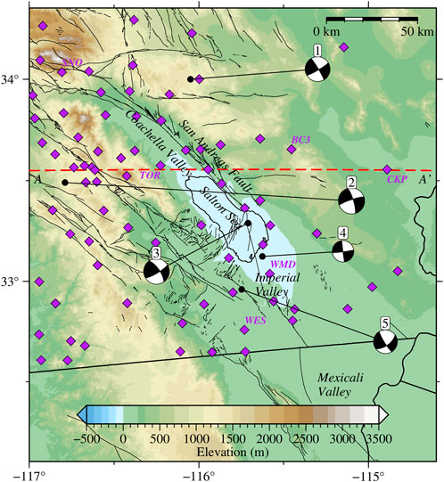
FIGURE 1. Source (black circles)-receiver (purple diamonds) geometry of the numerical experiment in Salton Trough. Beach balls show the focal mechanisms of the earthquakes (Table 1). Red dashed line is the A–A’ profile location in Figure 2. Labeled stations are considered in Figures 6–8.
2 Earth model space
To develop the context behind our approach to the current research and following Fichtner (2010), we give a brief introduction to the underdeveloped theory of the model space
and provide some relevant properties of the space. First, we note that the notion of admissible does not have a clear definition in the geoscience community. It can be a broad and complicated term in Earth science because the space can include models as simple as 1D models used to compute global earthquake locations and theoretical arrival times that would otherwise be impractical for other applications requiring more detail. For completeness, we define an admissible Earth model as geologically reasonable or has a practical use allowed to vary in complexity from global seismic phase identification to ground shaking estimation in earthquake engineering or natural resource exploration.
Each model
where
showing that each model can have different representations. The parameterization works for any given Earth model of differing scales by defining the material properties as zero at spatial locations where they are not available. An Earth model in southern California has model parameters undefined elsewhere, and a model that does not include topography is undefined above zero elevation. Since we use the spectral-element method (Komatitsch & Vilotte, 1998) for our wavefield simulations, the model parameters here are defined on the Gauss-Lobatto-Legendre (GLL) points in the mesh so that
The model space is infinite. Given any model
The models
3 Data and methods
3.1 Community velocity models
The two Earth models we evaluate in Salton Trough are the most recent versions of the community velocity models developed by the Southern California Earthquake Center (SCEC), namely Community Velocity Model—SCEC (CVM-S 4.26) (E. Lee, Chen, Jordan, et al., 2014) and Community Velocity Model—Harvard (CVM-H v15.1) (Tape et al., 2010; Shaw et al., 2015). CVM-S 4.26 was developed from its immediate predecessor through full-3D tomographic inversion using earthquake and noise correlation waveforms with a shortest period of 5 s. CVM-H v15.1 is constructed using earthquake-only adjoint tomography with a minimum period of 2 s. Both models deliver P and S wave velocities. Density is derived empirically from
We abbreviate CVM-S 4.26 and CVM-H v15.1 to cvms and cvmh for the remainder of the paper. We query the models using the Unified Community Velocity Model (UCVM) software (Small et al., 2017).
3.2 Model representations
The CVMs can be modified by including other parameters not in the original versions to enhance their performance. We focus on three add-ons, including topography, near-surface geotechnical layering, and anelastic attenuation. Consideration for these features resulted in 16 and 8 model representations for cvms and cvmh, respectively (Tables 2 and 3).
3.2.1 Topography
Some wave propagation solvers cannot explicitly handle complex spatial domains; thus, models developed with topography need to be flattened (Aagaard et al., 2008). Conversely, to use surface topography in solvers capable of incorporating them, the models without one need to be modified. We can consider both cases here since cvms was developed without topography (Figure 2A) while cvmh includes topography (Figure 2E).
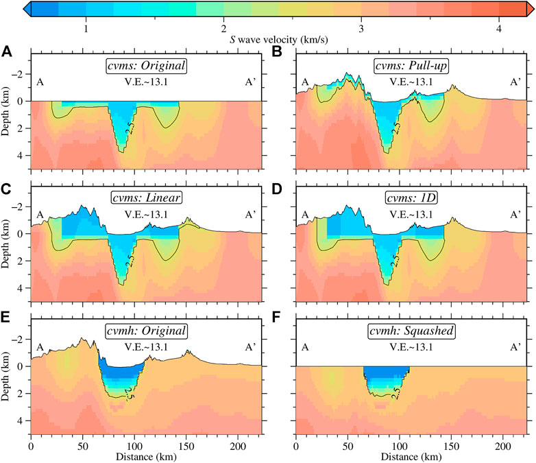
FIGURE 2. S wave velocity profiles of the community models along profile A-A′ in Figure 1 showing topographic representations considered in the study. (A) The original model for cvms developed without topography. (B) Pull-up model for cvms. (C) Linear model for cvms. (D) 1D model for cvms. (E) The original model for cvmh developed with topography. (F). Squashed model for cvmh.
The default method utilized by UCVM to include topography in cvms is to remap the parameters in the model following surface elevation variations (Pull-up in Figure 2B), i.e.,
where we show dependence for a model in
To preserve the shape of the geologic features in cvms when including topography, we experiment with linear (Figure 2C) and 1D (Figure 2D) extension models. These simple implementations fill the model between zero elevation and the free surface. The linear model extends cvms to the surface using an elevation-dependent gradient based on the values at zero depth and a set minimum velocity. The model becomes 1D whenever the zero-depth values or the interpolated model are lower than the predefined minimum velocities:
with
The 1D and linear models are queried with our modified UCVM software (Ajala, 2021), and we set the minimum P and S wave velocities in the implementation to 1,500 m/s and 800 m/s, respectively. As is easily observed, these models can quickly become unrealistic, especially if the original model has low velocities at zero depth in areas with high elevations creating inverted basin-like structures at high elevations (Figures 2C,D). These modifications also introduce sharp velocity contrasts in the model that may have an adverse effect on the wavefield prediction.
For the cvmh model with topography, we use the default UCVM representation to flatten the model by squashing the topographic variations to a planar surface (Figure 2F). This algorithm can be considered the reverse operation of the pull-up model, i.e.,
One drawback of using models developed with topography is differences may exist between the elevation models used in creating the models and any other elevation model that may be subsequently used (Figure 3). In the current case, cvmh was developed using an ∼1 km resolution USGS GTOPO30 model, while the elevation model in UCVM is the ∼30 m resolution USGS National Elevation Dataset. The mismatch between the two elevation models can misrepresent the model at the near surface. Additionally, the model top of cvmh representing the highest elevation at which model parameters are defined in the model does not always correspond to its surface elevation. According to Plesch et al. (2011), who describe the querying interface for the cvmh model, the cvmh free surface is the lower value between the surface elevation and the model top. When the model is queried at elevations with empty voxels, the free surface elevation is recursively reduced by 100–1,000 m until model parameters are found, further contributing to the near-surface artifacts. Figure 3 shows that up to 300 m differences can be found between the elevation models used by UCVM and cvmh.
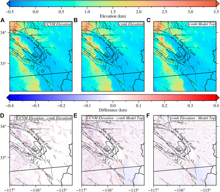
FIGURE 3. Elevation models used in UCVM and cvmh querying program. (A) ∼30 m resolution elevation model from the USGS National Elevation Dataset used by UCVM. (B) ∼1 km resolution elevation model from USGS GTOPO30 used by the cvmh program. (C) cvmh model top representing the highest elevation where elastic parameters are defined in the model. (D) Difference between UCVM elevation and cvmh elevation. (E) Difference between UCVM elevation and cvmh model top. (F) Difference between cvmh elevation and its model top. Black diamonds in (A) indicate the locations of the stations shown in Figure 6.
3.2.2 Near-surface modification
The model parameters in the shallow parts of the model may be modified to reflect the soft soils, sediments, and weathered materials relevant to ground motion studies but are often lost or unresolved during tomography, particularly at lower frequencies. We utilize the
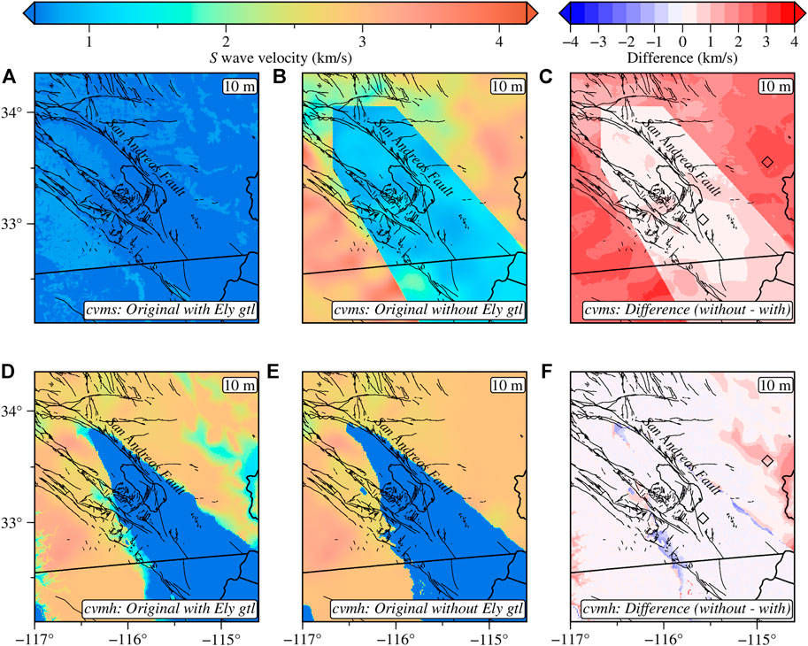
FIGURE 4. S wave velocity slices at 10 m depth showing the effect of partially including Ely geotechnical layer. Original cvms with geotechnical layering (A) and without geotechnical layering (B). (C) Difference between the models in (A) and (B). Original cvmh with geotechnical layering (D) and without geotechnical layering (E). (F) Difference between the models in (D) and (E). The two black diamonds in (C,F) indicate the locations of the stations used in Figure 7. The minimum and maximum S wave velocities shown are 0.6 km/s and 4.2 km/s, respectively.
3.2.3 Anelastic attenuation
Attenuation is imperative for accurate wavefield simulations, especially in areas with thick sedimentary basins where ground motion amplitudes can be overestimated. The developers of the cvmh and cvms models do not invert for anelastic attenuation when developing the models, so we implement a simple frequency-independent attenuation model. Attenuation is incorporated using the empirical Olsen relationship (Olsen et al., 2003) that determines the shear wave quality factor by scaling the S wave velocity,
and we use an Olsen attenuation ratio
3.3 Validation exercise
We conduct a seismic wavefield numerical experiment using past earthquakes to rank the prediction abilities of the different model representations developed. Our focus is on matching the observed waveforms. We refer to Ajala and Persaud (2021) for more details regarding the simulation setup.
3.3.1 Earthquake seismograms
We select five medium-magnitude (Mw3.6–4.4) earthquakes that are well recorded by three-component broadband seismometers in the region (Figure 1) and postdate any event used to develop cvmh and cvms (Table 1) from the updated catalog of Yang et al. (2012). Seismograms at each station are downloaded using the Southern California Earthquake Center (SCEDC) Seismogram Transfer Program (STP) and filtered in three period bands: 6–30, 3–30, and 2–30 s. Waveforms are selected for analysis if the signal-to-noise (SNR) ratio based on the amplitude and energy exceeds three on all components, which resulted in more waveforms with increasing frequency content (Tables 2 and 3).
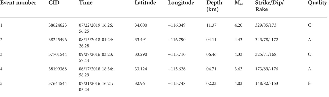
TABLE 1. Source parameters for the earthquakes used in the validation exercise. The event quality is related to nodal plane uncertainty of the focal mechanisms and the ranking scheme is described in Yang et al. (2012).
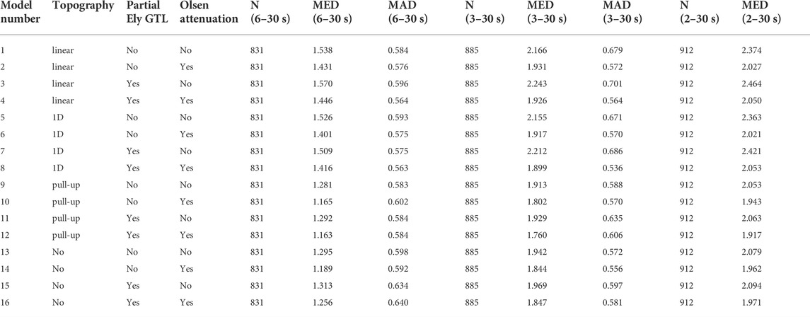
TABLE 2. Description of the model representations for cvms and their waveform misfit statistics. N—number of waveforms. MED—median waveform misfit. MAD—Median absolute deviation.
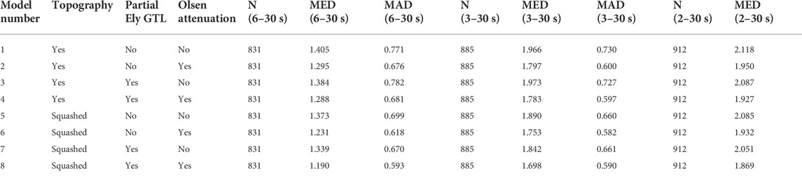
TABLE 3. Description of the model representations for cvmh and their waveform misfit statistics. N—number of waveforms. MED—median waveform misfit. MAD—Median absolute deviation.
3.3.2 Wave propagation simulation
We perform the simulations (Figure 5) using the SPECFEM3D package (Komatitsch & Vilotte, 1998). The earthquakes are represented as moment tensor point sources with focal mechanism parameters from Yang et al. (2012), and we do not perform source inversions. The source time functions are Gaussian, with widths equalling the half-duration of the events. In all models, the minimum S wave velocity is limited to 600 m/s to ensure that the simulations are accurate to a global minimum period of ∼2 s. Due to the velocity cut-off, we refer to our Ely geotechnical layering as partial since the near-surface velocities provided by the model can be as low as 90 m/s (Ely et al., 2010).
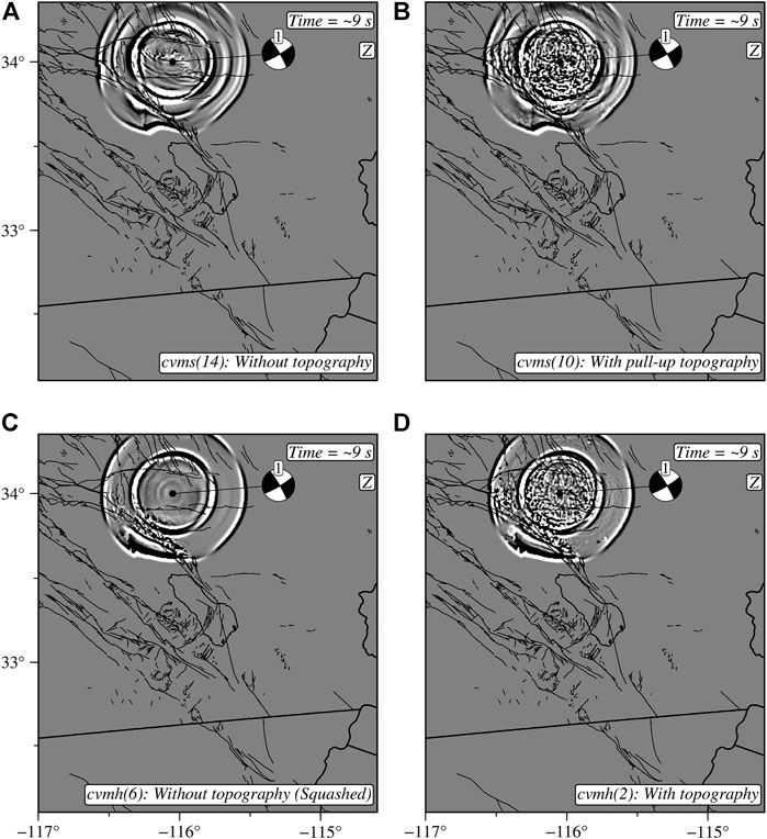
FIGURE 5. Wavefield simulation ∼9 s time step showing the effects of topography in the community models. Snapshot in cvms without topography (A) and with topography (B). Snapshots in cvmh without topography (C) and with topography (D). The models can be identified in Tables 2 and 3 using the numbers in the parenthesis next to model names in the bottom right labels.
3.3.3 Model evaluation
Following each simulation, we compute the misfit between the full waveform predictions made by the models
We use the median WM to determine the models’ performance and rank them.
To measure the sensitivity of the features we incorporate into the models, we compute the percentage change in the median WM between model pairs that differ only in those features. For example, to evaluate the sensitivity of the wavefield predictions for topography in the cvmh model (Table 3), we compute the misfit change for the following model pairs: (5, 1), (6, 2), (7, 3), and (8, 4), with positive percentage changes indicating an improved model. The range of percentage misfit change is used to assess the impact of the modifications or lack thereof on the model performance.
4 Results
As previously noted, a model representation is said to be better than another if it has a lower waveform misfit regardless of the magnitude. Figures 6–8 show waveform examples at different sites to communicate the variability of the simulation results. Figures 9, 10 summarize the validation exercise using the median WM. Each model realization can be considered as belonging to neighborhoods around the community models that non-tomographic modifications can generate. Thus, our goal is to provide insight into the importance of the model modifications using only a few elements of the model space and to avoid excessive computations.
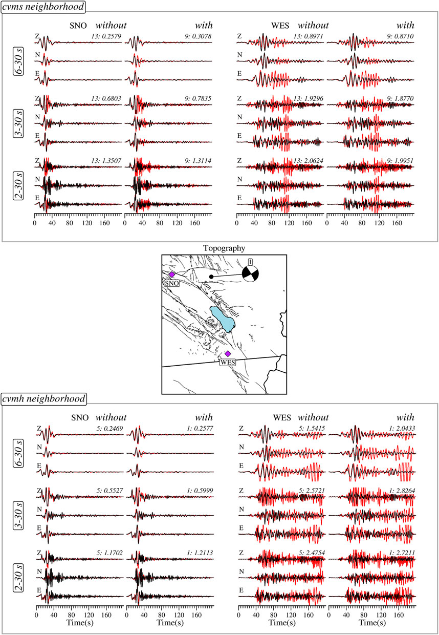
FIGURE 6. Observed (black) and synthetic (red) ground displacement records generated by the community models with (right columns) and without (left columns) topography at sites with (SNO) and without (WES) significant relief for different period bands. The top panel show waveforms for cvms and the bottom panel for cvmh. The middle panel shows the location of the earthquake and stations considered. The models can be identified by the number in the top right corner of each three-component record (Tables 2 and 3); the value following the colon is average waveform misfit over the three components. A lower misfit implies a better waveform prediction. Z—Vertical component. N—North-South component. E—East-West component.
Among other simplifications, since we use empirical relations to determine some of the model vectors such as density and anelastic attenuation and do not invert for source parameters, some of the misfits in the results may be incorrectly attributed to the features in question. We also note that an ideal investigation would utilize sources and receivers almost everywhere in the simulation domain, which is currently intractable. Thus, the results in this section are only valid for our selection of sources and stations where we have computed localized wavefield misfits. Finally, the low-frequency results evaluated at 6–30 s are most reliable because the community models are developed using waveforms in that range which is probably why the waveform misfit is significantly higher for shorter periods. However, the extension of our analysis to 2 s also addresses the common assumption that certain parameters may be more important at higher versus lower frequencies which is often postulated without knowledge of these results.
4.1 Topography effects
Figure 5 shows wavefield snapshots in the cvmh and cvms models, illustrating the scattering effects of topography. The waveform examples in Figure 6 show seismograms at two stations: SNO with an elevation of 2,339 m and WES at around 8 m. Since these two sites represent areas with significant topographic contrast, the results provide insight into the importance of an elevation model. We compare results in the cvmh and cvms representations with and without topography. At SNO, model 13 (Table 2) of cvms without topography has a lower waveform misfit at 6–30 and 3–30 s over model 9, which incorporates the pull-up topography model. However, at 2–30 s period, we see that model 9 performs better, showing our first important point about how validation results that are true at lower frequencies do not necessarily hold at higher frequencies. At station WES, model 9 consistently outperforms model 13. For cvmh models, model 5 (Table 3) without topography, i.e., squashed, has a lower waveform misfit for the three period ranges than model 1, which includes topography. Similar results are observed at station WES where model 5 has better waveform predictions than model 1. One explanation regarding the late spurious arrivals and anomalous amplitudes produced by the cvmh model is a combination of laterally reflected and basin-edge-generated surface waves coupled with the relatively low velocities within the basin (Lai et al., 2020). The waveform misfits here are significant enough to correlate the results to the increased amplification of the surface waves in model 1 that do not seem to be required by the observed data and thus may point to structural artifacts in the model.
The summary of the sensitivity of the wavefield prediction to topography for cvms is found by computing misfit changes between the following model pairs (Table 2) for the linear model: (13, 1), (14, 2), (15, 3), (16, 4), 1D model: (13, 5), (14, 6), (15, 7), (16, 8), and Pull-up model: (13, 9), (14, 10), (15, 11), (16, 12). The ranges of the misfit change for the three period bands are shown in the legends of Figure 9. Including linear or 1D topography remarkably deteriorates the predictions at 6–30 s by ∼20% for the linear model and ∼18% for the 1D model. At 3–30 s, the effect is reduced to ∼14% for the linear model and ∼12% for the 1D model but is higher at 2–30 s. In contrast, the pull-up topography model improves the waveform predictions up to ∼7% at 6–30 s but becomes less impactful at the shorter periods with a maximum improvement of ∼3% at 2–30 s. The lack of improvement of the pull-up topography model at 6–30 and 3–30 s for the Figure 6 example at station SNO shows the spatial variability of the results that cannot be expressed with the median WM alone, and there are always exceptional cases like this. Between the model pairs that include attenuation, the performance of the linear and 1D models gets closer, in performance, to the pull-up topography models and the models without topography. For the cvmh model, we compute the percentage changes between model pairs (5, 1), (6, 2), (7, 3), and (8, 4) (Figure 10). For the three period ranges, the models with topography underperform relative to the squashed models with the most significant increase in misfit of ∼8% at 6–30 s that decreases to ∼3% at 2–30 s. For both CVMs, the impact of topography decreases with increasing frequency.
4.2 Partial Ely geotechnical layering
Here, we compare waveforms at station WMD, where the GTL effect is minimal, and station CKP, where the effect is significant (Figures 4, 7) for both cvmh and cvms models. For cvms at station CKP, model 11 with GTL better matches the observed waveforms than model 9 without GTL for all period ranges. The results at station WMD are inconsistent, with model 9 underperforming at 6–30 s and outperforming at both 3–30 and 2–30 s compared to model 11. Cvmh model 1 without GTL underperforms relative to model 3 with GTL at station CKP for all period ranges. At station WMD, we have a situation opposite to that observed for the cvms model, with model 1 outperforming at 6–30 s but underperforming for the other two period ranges.
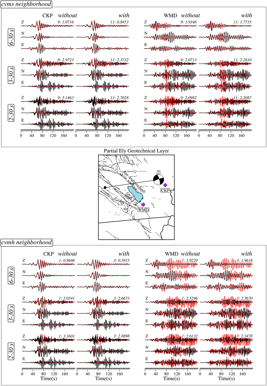
FIGURE 7. Observed (black) and synthetic (red) ground displacement records generated by the community models with (right columns) and without (left columns) Ely geotechnical layering at sites with (WMD) and without (CKP) significant model difference for different period bands. The top panel show waveforms for cvms and the bottom panel for cvmh. The middle panel shows the location of the earthquake and stations considered. The models can be identified by the number in the top right corner of each three-component record (Tables 2 and 3); the value following the colon is average waveform misfit over the three components. A lower misfit implies a better waveform prediction. Z—Vertical component. N—North-South component. E—East-West component.
For the summary results for cvms in Figure 9, we compute the change between pairs (1, 3), (2, 4), (5, 7), (6, 8), (9, 11), (10, 12), (13, 15), and (14, 16). For the three period bands, we have cases where including GTL provides an improved model and cases where it does not. In general, the percentage changes due to GTL is less than 6% for all model pairs, with the most significant deterioration in waveform prediction at 6–30 s. Model pair (10, 12) is the only one that consistently improves with the addition of GTL over all frequency bands and the only pair that improves at 3–30 s. For the cvmh model, we consider the following pairs: (1, 3), (2, 4), (5, 7), and (6, 8). Almost all the models improve when GTL is included, albeit with a relatively small percentage <3.4% besides the model pair (1, 3) at 3–30 s, which gives an ∼0.3% misfit increase.
4.3 Anelasticity
The waveform examples are for station TOR, located in the Coachella Valley basin, and station BC3 in the mountain ranges (Figure 8). Model 16 of cvms that includes Olsen attenuation significantly outperforms model 15 without attenuation at both sites. A similar scenario is observed for cvmh model 7 and model 8, where the effect of the attenuation model in balancing the amplitudes can be appreciated.
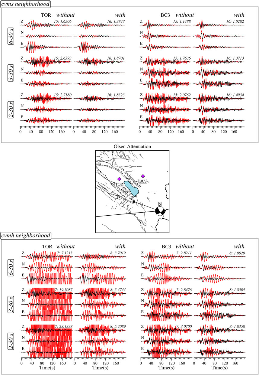
FIGURE 8. Observed (black) and synthetic (red) ground displacement records generated by the community models with (right columns) and without (left columns) attenuation at sites with (TOR) and without (BC3) significant basin sediments for different period bands. The top panel show waveforms for cvms and the bottom panel for cvmh. The middle panel shows the location of the earthquake and stations considered. The models can be identified by the number in the top right corner of each three-component record (Tables 2 and 3); the value following the colon is average waveform misfit over the three components. A lower misfit implies a better waveform prediction. Z—Vertical component. N—North-South component. E—East-West component.
In Figure 9 for cvms, we compute the change for the model pairs (1, 2), (3, 4), (5, 6), (7, 8), (9, 10), (11, 12), (13, 14), (15, 16). In all cases, the inclusion of attenuation provides a better model, with the results becoming more significant at shorter periods. We use the pairs (1, 2), (3, 4), (5, 6), and (7, 8) for cvmh (Figure 10) and get similar results to cvms. Incorporating attenuation improves the wavefield prediction abilities of the models and generally becomes more impactful at the higher frequencies than the other features that we explore in the model space.
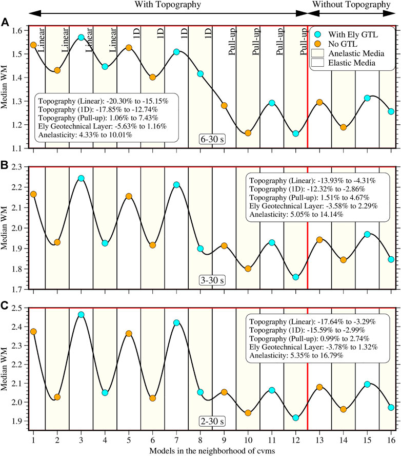
FIGURE 9. Validation result for the cvms models at 6–30 s (A), 3–30 s (B), and 2–30 s (C). Vertical axis represents the median waveform misfit and horizontal axis indicates the model number in Table 2. The red line demarcates the models with and without topography. The type of topographic representation is labeled at the top in (A). The statistics in the legend indicate the range in the waveform misfit percentage changes due to the inclusion of those features. Positive percentage change implies a global improvement in waveform predictions and vice versa.
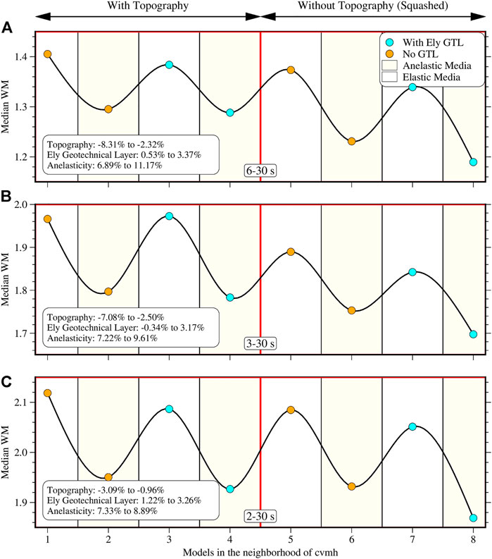
FIGURE 10. Validation result for the cvmh models at 6–30 s (A), 3–30 s (B), and 2–30 s (C). Vertical axis represents the median waveform misfit and horizontal axis indicates the model number in Table 3. The red line demarcates the models with and without topography. The statistics in the legend indicate the range in the waveform misfit percentage changes due to the inclusion of those features. Positive percentage change implies a global improvement in waveform predictions and vice versa.
5 Discussion
From our results, we are reminded that beyond simple models with analytical solutions, predictions about the performance of 3D heterogeneous Earth models should generally be avoided unless the claims are explicitly validated. Due to the complexity of model validation, the results presented are strictly valid only for the earthquakes-station distribution we have used, and our choice of the normalized classical waveform misfit function (Ajala & Persaud, 2021). Other error quantifiers such as Goodness-of-Fit (Olsen & Mayhew, 2010) favored by engineers or time-frequency misfit (Kristekovà et al., 2009) can and should be explored to check if the results are globally equivalent. Finally, modifications of the seismic velocities to construct Earth models with improved waveform predictions may not necessarily translate to geologically representative models. Therefore, the resulting models will require ground truthing for use in geological interpretations. Of all the modifications considered, the 1D and linear model add-ons represent the most geologically unfeasible features.
5.1 Expectations vs. reality
Contrary to previous studies that emphasize the importance of topography on accurate ground motion predictions, especially at higher frequencies, our validation results generally indicate the opposite, particularly for the elevation-referenced cvmh model. These results are not surprising since many of the previous claims are from theoretical studies that use earthquake scenarios and fail to ground truth their findings using actual recordings. At the shorter periods, we noted that the performance of the linear and 1D models for the cvms models that include attenuation began to rival the pull-up model and the models without topography. Intuitively, we expected that including these crude models in the shallow parts of the model, believed to be the most critical for ground motion prediction, with thickness as much as ∼3.5 km, should significantly deteriorate the wavefield. To an extent, they do for the longer periods at 6–30 s, and the most natural claim would suggest that the results would worsen at shorter periods, but Figure 9 shows the opposite. The inclusion of attenuation in these models seems to overshadow the shallow low-resolution layer’s adverse effects on the wavefield prediction and give comparable results to the better models.
Our implementation of the Ely geotechnical layer is partial since we cut off the minimum shear wave velocity in all model representations to 600 m/s even though velocities as low as 90 m/s can be implemented. We do this to reduce the computational cost of our simulations and to be able to consider several models. Therefore, our analysis of the effect of the Ely geotechnical layer is somewhat incomplete. Nevertheless, the results show that modifying the near-surface to reflect better the surface geological conditions do lead to perturbations in the wavefield predictions and, in some cases, lead to better wavefield predictions. If the computational resources are available, the effect of a complete geotechnical layer should be more thoroughly explored. Taborda et al. (2016) studied the effect of Ely GTL for the CVM-H model but had a velocity cutoff of 200 m/s.
Attenuation is the only modification that lives up to the expectations presented in the literature. From the longer periods to the relatively short period (∼2 s) that we consider, including attenuation produces a better model representation with improved waveform prediction ability that became more impactful at the higher frequencies. Although we use the Olsen attenuation model, other attenuation models (Lin, 2014) can and should be tested in the region to study the sensitivity.
5.2 Recommendation for tomography and simulations
Using the pull-up topography model that adapts the otherwise flat cvms model following elevation variations consistently produced better model representations for cvms. Conversely, the original cvmh model with topography consistently underperformed in wavefield prediction compared to the squashed model that flattens the model. Due to elevation discrepancies between topographic models that may cause near-surface artifacts in elevation-referenced models, our results suggest that community tomography models may in some cases be best developed without topography. Flat models do not have the near-surface querying difficulty that models with topography have. Flat models can also be readily adapted to any elevation model if care is taken with the near-surface representation. Other topography models designed to reduce the distortion of the subsurface, such as the squashed tapered model (Thomson et al., 2019) and the representation presented by Stone et al. (2022), where the model is stretched and compressed above a certain depth to match topographic variations remain unexplored in a validation exercise. Based on our results, we suggest that the cvms model in the Salton Trough region be implemented with the pull-up topography model, which is the default elevation query mode utilized by UCVM, and with attenuation. For the cvmh model, we recommend the representation without elevation using the squashed topography model, which is also the default depth query mode utilized by UCVM, with attenuation to reduce the effect of unwanted basin resonance in the model (Figure 8), and with Ely geotechnical layering. This cvmh model (8 in Table 3 and Figure 10) produces the best waveform prediction of the 24 model representations at 3–30 and 2–30 s.
6 Conclusion
We conduct a validation exercise for 24 model representations of two SCEC CVMs using five moderate-magnitude earthquakes in Salton Trough. The models were used to test the effect of topography, Ely geotechnical layering, and attenuation on seismic full waveform prediction over three period bands: 6–30, 3–30, and 2–30 s. The pull-up topography approach that adapts the flat cvms model to the surface elevation produces a better predictive model. However, the elevation-referenced cvmh model performs poorly relative to the flattened version using the squashed topography model. We, therefore, suggest that developing tomographic models without topography just like cvms and then using the pull-up topography model to implement any elevation model is a suitable approach for producing community models. Although the minimum velocity cutoff set in our simulations may have obscured some details in the geotechnical model, the Ely geotechnical layering had inconsistent effects. It led to a better model in some cases for cvms and most cases for the cvmh model. Attenuation is the only feature that behaves as expected by consistently producing better models and becoming more impactful at higher frequencies, where it significantly improves the performance of the cvms model with near-surface representations that use simple 1D and linear models.
Data availability statement
Data and codes to reproduce our results are publicly available on Zenodo (Ajala and Persaud, 2022). Additional statistical information about the study is included in the Supplementary Material.
Author contributions
RA and PP designed the study. RA performed the analysis and wrote the initial draft of the manuscript. All authors read, revised, and approved the final manuscript.
Funding
The research was funded by the NSF award 2105320 and SCEC awards 18074, 19014, 20023, 21059. RA was also supported by the Society of Exploration Geophysicists merit-based scholarship and PP was supported as a 2020-21 fellow of the Radcliffe Institute for Advanced Study at Harvard University.
Acknowledgments
We thank editors, Jonas D. De Basabe and Fernando Lopez-Caballero, and reviewers, Filippo Gatti and Vladimir Tcheverda for their thorough reviews and comments which helped to improve the manuscript. All figures are plotted using the Generic Mapping Tools (Wessel et al., 2019). The SPECFEM3D package (Komatitsch & Vilotte, 1998) is used for the waveform simulations. The SCEC contribution number for this paper is 11904.
Conflict of interest
The authors declare that the research was conducted in the absence of any commercial or financial relationships that could be construed as a potential conflict of interest.
Publisher’s note
All claims expressed in this article are solely those of the authors and do not necessarily represent those of their affiliated organizations, or those of the publisher, the editors and the reviewers. Any product that may be evaluated in this article, or claim that may be made by its manufacturer, is not guaranteed or endorsed by the publisher.
Supplementary material
The Supplementary Material for this article can be found online at: https://www.frontiersin.org/articles/10.3389/feart.2022.964806/full#supplementary-material
References
Aagaard, B. T., Brocher, T. M., Dolenc, D., Dreger, D., Graves, R. W., Harmsen, S., et al. (2008). Ground-motion modeling of the 1906 san francisco earthquake, part I: Validation using the 1989 loma Prieta earthquake. Bull. Seismol. Soc. Am. 98 (2), 989–1011. doi:10.1785/0120060409
Ajala, R. (2021). Modified UCVM software with blending functionality: Zenodo. Retrieved from. doi:10.5281/zenodo.4533337
Ajala, R., and Persaud, P. (2022). Code and data repository for the role of topography, geotechnical layering, and attenuation on ground motion prediction: Zenodo. Retrieved from. doi:10.5281/zenodo.6615706
Ajala, R., and Persaud, P. (2021). Effect of merging multiscale models on seismic wavefield predictions near the southern san Andreas fault. JGR. Solid Earth 126, 1–23. doi:10.1029/2021jb021915
Brocher, T. M. (2005). Empirical relations between elastic wavespeeds and density in the earth’s crust. Bull. Seismol. Soc. Am. 95 (6), 2081–2092. doi:10.1785/0120050077
Ely, G. P., Small, P., Jordan, T. H., Maechling, P. J., and Wang, F. (2010). A Vs30-derived near-surface seismic velocity model. San Francisco, CA: AGU Fall Meeting. Paper presented at the.
Fichtner, A., and Zunino, A. (2019). Hamiltonian nullspace shuttles. Geophys. Res. Lett. 46, 644–651. doi:10.1029/2018gl080931
Graves, R. W., Aagaard, B. T., and Hudnut, K. W. (2011). The ShakeOut earthquake source and ground motion simulations. Earthq. Spectra 27 (2), 273–291. doi:10.1193/1.3570677
Igel, H. (2017). Computational Seismology: A practical introduction. New York, USA: Oxford University Press.
Jones, L. M., Bernknopf, R., Cox, D., Goltz, J., Hudnut, K., Mileti, D., et al. (2008). The ShakeOut scenario. Reston, VA: USGS Open File. Report 2008-1150.
Juarez, A., and Ben-Zion, Y. (2020). Effects of shallow-velocity reductions on 3D propagation of seismic waves. Seismol. Res. Lett. 91, 3313–3322. doi:10.1785/0220200183
Komatitsch, D., and Vilotte, J. (1998). The spectral element method: An efficient tool to simulate the seismic response of 2D and 3D geological structures. Bull. Seismol. Am. 88 (2), 368–392.
Kristekovà, M., Kristek, J., and Moczo, P. (2009). Time-frequency misfit and goodness-of-fit criteria for quantitative comparison of time signals. Geophys. J. Int. 178, 813–825. doi:10.1111/j.1365-246x.2009.04177.x
Lai, V., Graves, R., Yu, C., Zhan, Z., and Helmberger, D. V. (2020). Shallow basin structure and attenuation are key to predicting long shaking duration in Los Angeles basin. J. Geophys. Res. Solid Earth 125, 1–15. doi:10.1029/2020jb019663
Lee, E., Chen, P., Jordan, T. H., Maechling, P. B., Denolle, M. A., and Beroza, G. C. (2014). Full-3-D tomography for crustal structure in Southern California based on the scattering-integral and the adjoint-wavefield methods. J. Geophys. Res. Solid Earth 119 (8), 6421–6451. doi:10.1002/2014jb011346
Lee, E., Chen, P., and Jordan, T. H. (2014). Testing waveform predictions of 3D velocity models against two recent Los Angeles earthquakes. Seismol. Res. Lett. 85 (6), 1275–1284. doi:10.1785/0220140093
Lee, S., Chan, Y., Komatitsch, D., Huang, B., and Tromp, J. (2009). Effects of realistic surface topography on seismic ground motion in the yangminshan region of taiwan based upon the spectral-element method and LiDAR DTM. Bull. Seismol. Soc. Am. 99 (2A), 681–693. doi:10.1785/0120080264
Lee, S., Chen, H., Liu, Q., Komatitsch, D., Huang, B., and Tromp, J. (2008). Three-dimensional simulations of seismic-wave propagation in the Taipei basin with realistic topography based upon the spectral-element method. Bull. Seismol. Soc. Am. 98 (1), 253–264. doi:10.1785/0120070033
Lee, S., Komatitsch, D., Huang, B., and Tromp, J. (2009). Effects of topography on seismic-wave propagation: An example from northern Taiwan. Bull. Seismol. Soc. Am. 99 (1), 314–325. doi:10.1785/0120080020
Lin, G. (2014). Three-Dimensional compressional attenuation model (QP) for the Salton Trough, southern California. Bull. Seismol. Soc. Am. 104 (5), 2579–2586. doi:10.1785/0120140049
Miller, U. (2014). The effect of topography on the seismic wavefield. Alaska: University of Alaska Fairbanks.
Olsen, K. B., Day, S. M., and Bradley, C. R. (2003). Estimation of Q for long-period (> 2 sec) waves in the Los Angeles basin. Bull. Seismol. Soc. Am. 93 (2), 627–638. doi:10.1785/0120020135
Olsen, K. B., and Mayhew, J. E. (2010). Goodness-of-fit criteria for broadband synthetic seismograms, with application to the 2008 Mw 5.4 chino hills, California, earthquake. Seismol. Res. Lett. 81 (5), 715–723. doi:10.1785/gssrl.81.5.715
Plesch, A., Tape, C., Shaw, J. H., Small, P., Ely, G., and Jordan, T. (2011). User guide for the southern California earthquake center community velocity model: Scec cvm-H 11.9.0.
Restrepo, D., Bielak, J., Serrano, R., Gomez, J., and Jaramillo, J. (2016). Effects of realistic topography on the ground motion of the Colombian Andes - a case study at the Aburra Valley, Antioquia. Geophys. J. Int. 204, 1801–1816. doi:10.1093/gji/ggv556
Shaw, J. H., Plesch, A., Tape, C., Suess, M., Jordan, H., Ely, G., et al. (2015). Unified Structural Representation of the southern California crust and upper mantle. Earth Planet. Sci. Lett. 415, 1–15. doi:10.1016/j.epsl.2015.01.016
Small, P., Gill, D., Maechling, P., Taborda, R., Callaghan, S., Jordan, T., et al. (2017). The SCEC unified community velocity model software framework. Seismol. Res. Lett. 88 (6), 1539–1552. doi:10.1785/0220170082
Stone, I., Wirth, E. A., and Frankel, A. (2022). Topographic response to simulated Mw 6.5-7.0 earthquakes on the seattle fault. Bulletin of the Seismological of America, 1–27.
Taborda, R., Azizzadeh-Roodpish, S., Khoshnevis, N., and Cheng, K. (2016). Evaluation of the southern California seismic velocity models through simulation of recorded events. Geophys. J. Int. 205, 1342–1364. doi:10.1093/gji/ggw085
Tape, C., Liu, Q., Maggi, A., and Tromp, J. (2010). Seismic tomography of the southern California crust based on spectral-element and adjoint methods. Geophys. J. Int. 180 (1), 433–462. doi:10.1111/j.1365-246x.2009.04429.x
Thomson, E. M., Bradley, B. A., and Lee, R. L. (2019). Methodology and computational implementation of a New Zealand velocity model (NZVM2.0) for broadband ground motion simulation. N. Z. J. Geol. Geophys. 63, 110–127. doi:10.1080/00288306.2019.1636830
Tromp, J. (2020). Seismic wavefield imaging of Earth’s interior across scales. Nat. Rev. Earth Environ. 1, 40–53. doi:10.1038/s43017-019-0003-8
Virieux, J., and Operto, S. (2009). An overview of full-waveform inversion in exploration geophysics. GEOPHYSICS 74, 1–26. doi:10.1190/1.3238367
Wessel, P., Luis, J. F., Uieda, L., Scharroo, R., Wobbe, F., Smith, W. H. F., et al. (2019). The generic mapping tools version 6. Geochem. Geophys. Geosyst. 20, 5556–5564. doi:10.1029/2019gc008515
Keywords: seismic hazard, computational seismology, waveform prediction, topography, anelastic attenuation, geotechnical layering, model space, model validation
Citation: Ajala R, Persaud P and Juarez A (2022) Earth model-space exploration in Southern California: Influence of topography, geotechnical layer, and attenuation on wavefield accuracy. Front. Earth Sci. 10:964806. doi: 10.3389/feart.2022.964806
Received: 09 June 2022; Accepted: 25 August 2022;
Published: 29 September 2022.
Edited by:
Jonas D. De Basabe, Center for Scientific Research and Higher Education in Ensenada (CICESE), MexicoReviewed by:
Filippo Gatti, Université Paris-Saclay, FranceVladimir Tcheverda, Institute of Petroleum Geology and Geophysics (RAS), Russia
Copyright © 2022 Ajala, Persaud and Juarez. This is an open-access article distributed under the terms of the Creative Commons Attribution License (CC BY). The use, distribution or reproduction in other forums is permitted, provided the original author(s) and the copyright owner(s) are credited and that the original publication in this journal is cited, in accordance with accepted academic practice. No use, distribution or reproduction is permitted which does not comply with these terms.
*Correspondence: Rasheed Ajala, cmFqYWxhMUBsc3UuZWR1