 Aihua Ye
 Zhipeng Zhu
 Ruyi Zhang
 Ziniu Xiao
 Limin Zhou
- 1Key Laboratory of Geographic Information Science, Ministry of Education, East China Normal University, Shanghai, China
- 2State Key Laboratory of Numerical Modelling for Atmospheric Sciences and Geophysical Fluid Dynamics, Institute of Atmospheric Physics, Beijing, China
- 3Institute of Eco-Chongming, Shanghai, China
There is a growing debate regarding the influence of solar activity on climate change as the solar forcing signal on decadal/multidecadal timescales is not robust in long-term reconstructed climate data or numerical simulations. However, solar forcing could be amplified by ocean–atmosphere coupling in sensitive regions, including the North Atlantic Ocean (N.A.). This study assessed the influence of varied total solar irradiance (TSI) due to the effects of solar activity on Atlantic Meridional Overturning Circulation (AMOC) based on an Earth System model with intermediate complexity (PLASIM-GENIE). Three groups of experiments with different TSI series; i.e., constant (NS), decadal varied (DS), and reconstructed whole (AS) for 1610–2000, were conducted and the AMOC response was investigated. The results showed that the internal forcing of the climate system led to quasi-35-year and quasi-65-year AMOC cycles and a significant and stable negative correlation between TSI and AMOC on a multidecadal timescale. The period was significantly extended due to solar forcing. The declining AMOC trend occurred in simulations after 1800. Thus, solar forcing contributed to a weakening AMOC at a rate of 0.41 Sv per century. The decadal variation in TSI was the main contributor to this decline due to solar forcing.
1 Introduction
Evidence from observations and geologic proxies indicates that solar forcing is among the key natural driving forces affecting decadal/multidecadal climate variation (Eddy, 1976; Haigh, 1996; Wang et al., 2005; Liu et al., 2013; Gray et al., 2018; Xu et al., 2019; Kuroda et al., 2022). Although various linking mechanisms have been proposed, such as the “top-down” regime (stratospheric ozone ultraviolet radiation effect) or “bottom-up” regime (total radiation irradiance effect) (Haigh, 1994; Gray et al., 2009; Mann et al., 2009), recent studies based on climate models or reconstructed long-term reanalysis data have challenged the certainty of this linkage. A robust solar signal on decadal climate change was lacking in the long-term reanalysis or modeling data. Previous studies occasionally observed this linkage (Sjolte et al., 2018). Instead of solar forcing, volcanic eruptions or internal driving forces could also induce decadal climate variations (Mann et al., 2021). Consequently, the Sixth Assessment Report of the Intergovernmental Panel on Climate Change (IPCC-AR6) suggested that there exists great uncertainty regarding the influence of solar activity on decadal/multidecadal climate changes (Masson-Delmotte, 2021). The key to addressing this contradiction is to establish robust linking mechanisms between solar activity and climate systems.
Although the total solar irradiance (TSI) only fluctuates by approximately 0.1%–0.2% in the solar cycle of the 11-year Schwabe cycle (Foukal et al., 2006), the changes could accumulate and be amplified in sensitive ocean regions and lead to significant impacts on regional or even global climate. The North Atlantic Ocean region (N.A.) is considered a sensitive region (Gray et al., 2013; Scaife et al., 2013; Andrews et al., 2015; Cheng et al., 2016). Andrews et al. (2015) and Gray et al. (2016) declared that the accumulated solar energy in the mixed layer of the N.A. could generate a response lag of 3–4 years of surface pressure to the decadal solar cycle. In the N.A., the local ocean response could cause a global climate effect due to thermohaline circulation. Many studies have suggested that the Atlantic Meridional Overturning Circulation (AMOC) plays an important role in Atlantic multidecadal variability. Atlantic hurricane activity, frequency of drought events in the United States, and changes in rainfall in Europe and the East Asian summer monsoon are all reportedly related to the AMOC (Delworth et al., 1993; Timmermann et al., 1998; Sutton and Hodson, 2005; Zhang and Delworth, 2006; Yu Lei, 2009; Ting et al., 2011). Thus, the connection between solar forcing and the AMOC seems to be an important part of transmitting solar signals in climate systems (Shindell et al., 2001; Scaife et al., 2013).
Moreover, the AMOC fluctuates on variable timescales; i.e., from decadal to centennial to millennial (Zhang, 2008; Chylek et al., 2012; Park and Latif, 2012). Geological proxy records (Ran Lihua, 2008; Liu Jing, 2014; Zhao Yun, 2015; Li Dongling, 2016) and model simulations (Jiang et al., 2014) reveal the significant relationship between the AMOC and variations in sea surface temperature (SST) and ice sheets in the N.A. on a millennial scale. Lin et al. (2019) claimed that the AMOC shows two groups of decadal/multidecadal oscillations of 10–30 years and 50–80 years and that the formation of these two oscillations accounted for internal oscillation and trans-basin processes in the N.A. Bagatinsky and Diansky (2021) revealed that the Atlantic multidecadal oscillation was associated with the AMOC sinking branch at 60°N latitude and the rising branch at 25°N latitude and was part of a quasi-60-year cycle. Additionally, the multidecadal variation in AMOC would shift with global climate background changes (Cheng et al., 2016).
Various mechanisms of AMOC multidecadal fluctuation due to internal or external forcings have been proposed (Gregory et al., 2005; Yu et al., 2010; Lynch-Stieglitz, 2017). The meridional density gradient (Lee and Wang, 2010; Huang et al., 2014), fresh water flux, and deep convective variation (Sutton and Hodson, 2005) control the variation in AMOC by changing the N.A. SST and salinity. Solar activity could contribute to these factors by impacting the heat capacity, planetary waves (Huck et al., 2001), and melted sea–ice freshwater injections (Yu et al., 2010; Lynch-Stieglitz, 2017).
The relationship between AMOC and TSI, controlled by orbital factors or solar activity, has been studied through observations and model simulations. Paleoclimatic evidence from deep-sea cores indicated that the AMOC decreases with weakened solar radiation on a millennium timescale (Negre et al., 2010). Based on reconstructed N.A. climate data over the past 200 years, Gary et al. (2010) proposed that TSI can affect the AMOC on a decadal time scale through the storage of solar energy in the mixed layer in the N.A. region (Gray et al., 2010; Ineson et al., 2011; Scaife et al., 2013; Andrews et al., 2015). Numerical simulations by Scaife et al. (2013) also concluded that the AMOC could amplify the solar signal and shape the regional response patterns in the N.A. region. Menary and Scaife (2014) operated 150-year experiments with the HadGEM2-ES (Hadley Centre Global Environment Model 2, with Earth System components) model and found that increased TSI could affect atmospheric circulation by changing SST on the multidecadal timescale. Consequently, the impact on seawater evaporation and ocean stratification in the N.A. leads to AMOC enhancement. However, simulations by Muthers et al. (2016) based on the SOCOL-MPIOM model demonstrated that weakened TSI was followed by colder SST and enhanced sea–ice cover, which would increase the N.A. upper water density and speed the AMOC on a multidecadal time scale. However, a weakened TSI could also induce a negative AO phase, which could decrease the AMOC intensity. Other modeling results also revealed that TSI variation could cause either positive or negative effects on the strength of AMOC on different time scales (Zorita et al., 2004; Goosse and Renssen, 2006; Sedlacek and Mysak, 2009; Swingedouw et al., 2011).
The weakening trend of the AMOC has been detected by observations (Holliday et al., 2020) and paleoclimate proxies (Caesar et al., 2021). Although there is an argument for the origin of the weakening of the AMOC, the fluctuation in eddies (Lozier et al., 2019), internal tides (de Lavergne et al., 2017), and wind forcing (Swingedouw et al., 2022), in other words, internal or external forcing, are the main contributors to this weakening trend. Solar forcing with TSI variability on multiple timescales could affect the weakening trend of the AMOC; however, its contribution has not been fully investigated.
Regarding simulation of the AMOC, although the climate model with a high-resolution ocean part, in which eddies are permitted, could simulate key processes of the AMOC, such as the transformation of water masses, strong biases remain due to the possible serious underestimation of some uncertainties (Jackson et al., 2020). The coarse-resolution model could capture the first order of driving the AMOC (Swingedouw et al., 2022), the results of which may be more consistent with the present observations. Therefore, the solar forcing effect on AMOC is still useful for initial testing with the coarse-resolution model.
In this article, we use a coupled intermediate complexity earth system model, PLASIM-GENIE, to explore the influence of varied TSIs with multi-timescale (decadal to centennial) cycles on the AMOC. The model can operate the first order of the driving process and provide the main characteristics of the climate system, in which the ocean and sea–ice modules can well simulate AMOC variability. It is suitable for long-term large-scale ensemble studies.
Concretely, we designed 390-year single-factor forcing simulation experiments with different time scale variations in TSI based on the reconstructed series and investigated the responses of the AMOC. The structure of this article is as follows: the second section describes the climate model and experimental design; the third section provides experimental results and discussion; and the fourth section provides the conclusion.
2 Model and experimental setup
2.1 Model
This study used an Earth system model with intermediate complexity (PLASIM-Genie version 1.0), which coupled the planetary simulator (PLASIM) and ocean (GOLDSTEIN), sea ice (GOLDSTEINSEAICE), and land surface components (GENIE Earth System model), and can reproduce the main feature of the climate system (Marsh et al., 2004; Zorita et al., 2004).
The primitive equation of the atmosphere includes chaotic, three-dimensional (3-D) motion and interactive radiation and cloud cover, and dominates the computational load compared to the relatively simpler frictional geostrophic ocean, which neglects momentum advection. This model is suitable for long-term or global-scale comprehensive simulations. Based on the original slab ocean and sea–ice module with flux correction, the model tuned each module, which allowed the model to improve the prediction of the characteristics of ocean circulation and the climate system. The GOLDSTEIN sub-model can adopt surface wind speed, net energy, and net humidity fluxes provided by PLASIM-GENIE, perform relevant sea–ice correction, and output responses such as SST, salinity, and sea–ice thickness. GOLDSTEIN also improves the vapor transport process, which can not only represent the variability in ocean currents, such as AMOC caused by changes in the ocean interior, but also simulate the variability in AMOC driven by wind.
The PLASIM-GENIE model has a horizontal resolution of T21 (5.6°x5.6°, 32x64) (Lenton et al., 2007). Marsh et al. (2004) successfully investigated the operating pattern of thermohalines on decadal to millennial time scales with the GENIE model. PLASIM has a vertical resolution of 10 layers for the top at the tropopause. GOLDSTEIN has a vertical resolution of 32 layers, from the ocean surface down to the bottom. Compared to other EMICs, such as OSUVic, PLASIM-GENIE performs moisture flux adjustment, and a weak (9Sv) AMOC can be simulated. Holden et al. (2016)provided a more detailed description and model evaluation.
2.2 Experimental design
This study performed three experimental tests with different series of TSI. Figure 1 shows the five series of decomposed TSI reconstructed by Lean (2010) using the empirical mode decomposition (EMD) method. Figure 2 lists the three reconstructed TSI series in the simulations. The gray line represents the constant solar irradiance of 1364.6 W/m2 (NS). The blue line represents the original reconstructed TSI (AS). The red line represents the solar irradiance without 100-year and 22-year fluctuations, which is combined with the decomposed series of EMD1, EMD2, and EMD5 and calibrated with the mean of 1364.6 W/m2 (DS).
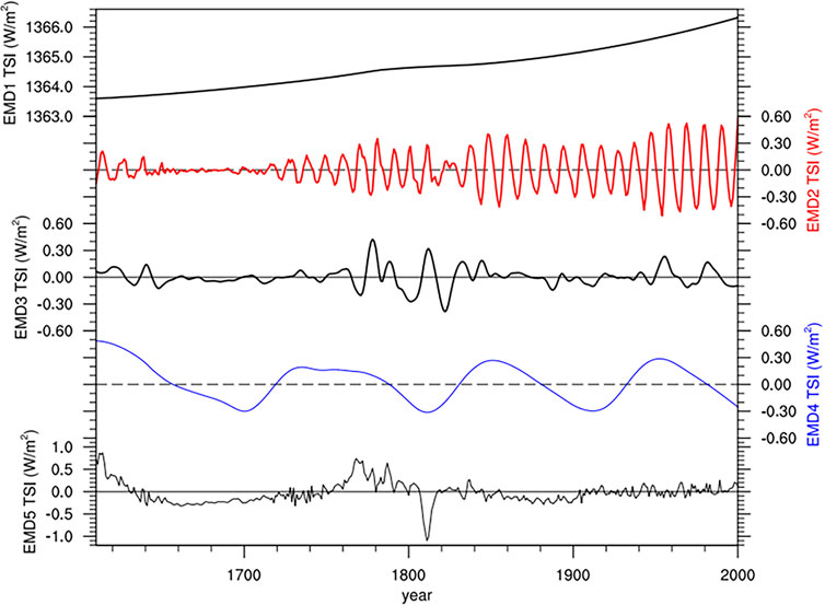
FIGURE 1. Five TSI EMD sequences used for reconstruction. EMD2 has a significant 11-year cycle. EMD4 has a significant 100-year cycle. EMD5 is the random item.
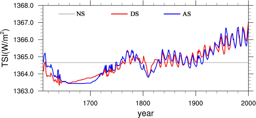
FIGURE 2. Three TSI sequences used for model forcing. NS: constant 1364.66 W/m2 (gray); DS: combination of EMD1, EMD2, and EMD5 (red); AS: combination of the entire sequence, which is the TSI reconstructed by Lean (2010).
Figure 3 shows the results of wavelet analysis of DS (panel a) and AS (panel b) with a significant 11-year period fluctuation in the DS series and significant quasi-11-year and centennial period variations in the AS series.
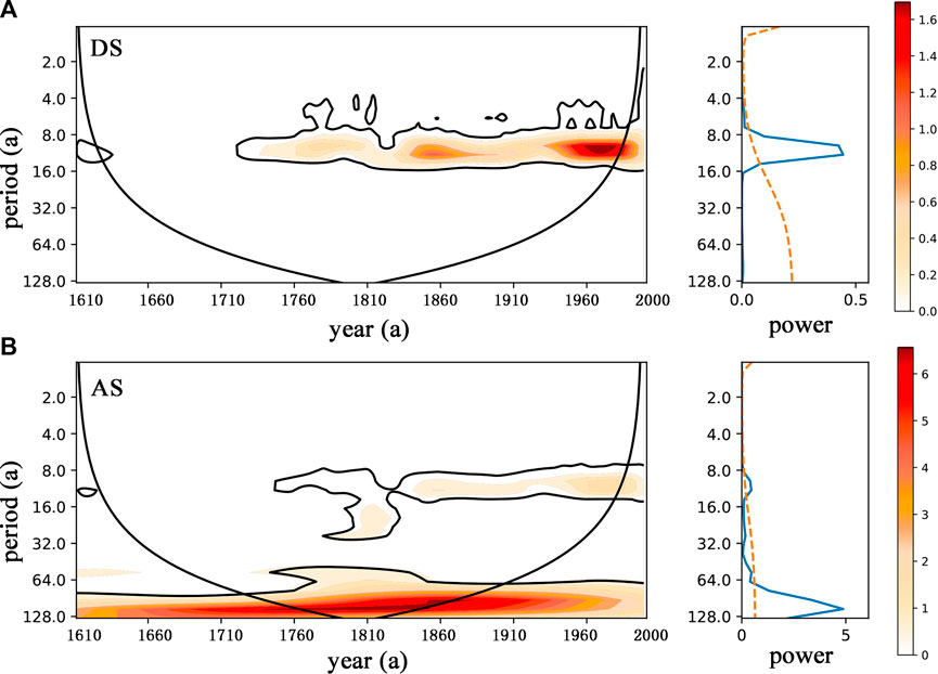
FIGURE 3. Wavelet analysis of TSI for the DS (A) and AS (B) tests. (Data are detrended. The dotted orange line is the 95% significance test).
To exclude the influence of human activity, other initial atmospheric parameters of simulations were kept at a constant value in 1850, i.e., the CO2 concentration was maintained at 280 ppm, which was the atmospheric CO2 concentration during the Holocene interglaciation (Lourantou et al., 2010). This value is often used as the equilibrium concentration of CO2 in idealized experiments (Eby et al., 2013).
Each test used three ensembles. The initial 200 years running with a constant solar irradiance of 1364.6 W/m2 are carried out in each group of simulations to make the model run stably. The annual averaged results of the simulation are output.
3 Results
3.1 Comparison with reanalysis data
The EN4 surface/subsurface temperatures and salinity dataset of the global oceans from the Hadley Center was used to evaluate the simulation results. Since the reanalysis data only cover the period from 1900 to 2022, the 1900–2000 temperature and salinity from the AS test were used for comparison.
Figure 4 shows the comparison of annual mean temperature and salinity at the surface and subsurface layers between the EN4 and AS tests, with SST shown in panels (a) and (c), subsurface sea temperature (300-meter-depth) shown in panels (b) and (d), sea surface salinity shown in panels (e) and (g), and subsurface sea salinity (300-meter-depth) shown in panels (f) and (h). The main spatial patterns of the whole-period averaged sea temperature and salinity were consistent between the reanalysis data and the simulation results. The surface salinity results of the simulation at the middle and low latitudes in the South Atlantic Ocean were lower. Based on previous model assessments (Liu et al., 2013; Holden et al., 2016), the PLASIM-GENIE model used in our work was able to reproduce the main features of the climate system in the Atlantic Ocean.
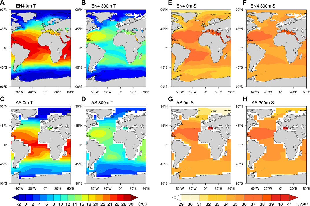
FIGURE 4. Results of the EN4 (top) and AS tests (bottom) from 1900 to 2000. Annual mean sea temperature at the surface (panels (A,C)) and 300 m depth (panels (B,D)). Annual mean sea salinity at the surface (panel (E,G)) and 300 m depth (panel (F,H)).
The temperature and salinity changes in the North Atlantic region from 1900 to 2000 were analyzed, as shown in Figure 5. The regional average temperature and salinity were standardized, which showed that the changes in the SST in the AS test were basically consistent with those observed during the whole period (Figure 5A). However, because the design of the model is not completely consistent with the actual climate change, certain differences in the trend changes of SST were observed in the last 10 years. After correlation analysis, the two sequences had a positive correlation of 0.272 by the 99% significance test for an EN4 SST lag of 3 years. SSS changes over the entire North Atlantic region were simulated poorly compared to temperature, with no significant correlation (Figure omitted). However, we further considered the changes over the small range of the sub-polar North Atlantic region (60oN–90oN, 80oW–30oE) where sea ice influence is significant in the AS test and EN4 datasets, and found a good correlation between the two. As shown in Figure 5B, the SSS changes of the two groups of data are very similar, with a positive correlation of 0.375 that passes the 99% significance test. Therefore, from the perspective of time change, the model well simulated the temperature and salinity changes in the North Atlantic region, which provides a basis for further analysis of AMOC changes.
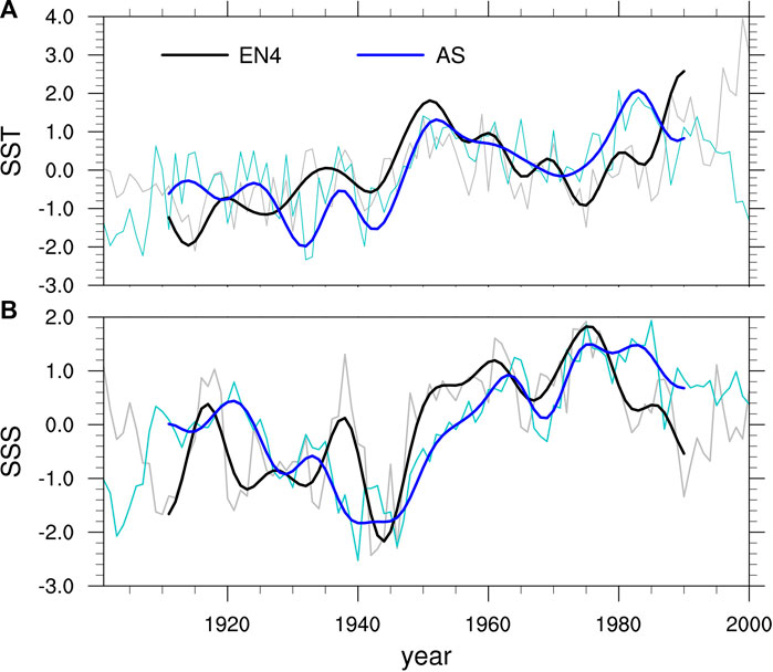
FIGURE 5. SST and SSS time sequences in the North Atlantic region of the AS test and EN4 dataset. (A) SST variation in the North Atlantic region (0oN–90oN, 80oW–30oE). (B) SSS variation in the subpolar North Atlantic region (60oN–90oN, 80oW–30oE). The data were all standardized.
3.2 Long-term response of the AMOC
Lozier et al. (2019) defined the AMOC index (AMOCI) as the maximum value of the overturning stream function in the density space. Other studies also selected the maximum value of the overturning stream function at a certain latitude as the AMOC index (Huang et al., 2014; Menary and Scaife, 2014; Cheng et al., 2016). In our work, the maximum value of the overturning stream function in the depth profile at 48°N was set as the AMOCI. Figure 6 shows the mean AMOCI of the three tests with 11 years of smoothing, with a fitting curve from 1800 to 2000. The gray line is the NS test, the red line is the DS, and the blue line is the AS. The AMOCI of the NS varied between 12.16 Sv and 18.83 Sv (Sv:1 Sverdrup = 1×10⁶ m3/s(−1)), with a mean of 15.3 ± 1.27 Sv. The results of the DS and AS tests showed mean AMOC strengths of 15.21 ± 0.63 Sv and 15.23 ± 0.57 Sv, respectively.
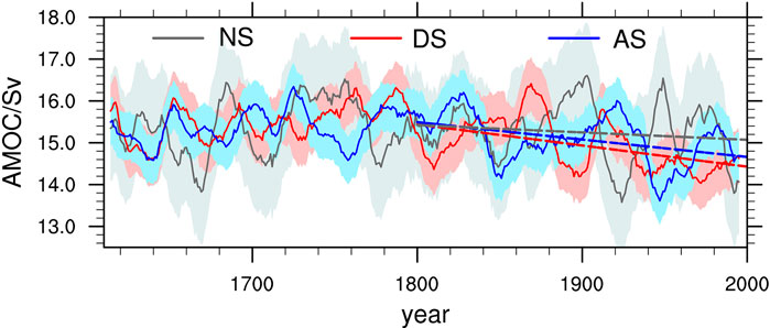
FIGURE 6. Eleven-year smoothed AMOCI for the composite mean of the three groups. NS is represented in gray; DS, in red; and AS, in blue. The shadow is the standard deviation of the AMOCI. The dashed line is the fitting curve of the AMOCI from 1800 to 2000.
The AMOCI of the NS test was consistent with the control run results by the Kiel Climate Model, in which the variation range of the AMOCI was 11–18 Sv (Park and Latif, 2012). The preindustrial control simulation in the HadGEM2-ES climate model had a mean AMOC strength of 13.6 ± 1.0 Sv (Menary et al., 2013). Menary and Scaife (2014) studied the influence of external forcings, such as volcanic eruptions and solar radiation, on the multidecadal AMOC change and found that the AMOC with multidecadal oscillation fluctuated between 12 Sv and 15 Sv during their 140-year experimental period. Compared with the recent observation dataset of the Rapid Climate Change (RAPID) program (AMOC intensity =18 ± 2.1 Sv) (Kanzow et al., 2010), the value of the NS experiment was slightly smaller. This result may be caused by the setting of other experimental conditions; for example, the fixed CO2 concentration, to preindustrial values.
The fitting curve in Figure 6 shows an obviously declining centennial trend after 1800. In the DS test, the largest weakening trend was observed, with a decline rate of 0.51 Sv per hundred years (Sv/100a), while the values were 0.41 Sv/(100a) in the AS test and 0.18 Sv/(100a) in the NS test. That is, the AMOCI in the DS test decreased the most, followed by the AS test, while the NS test decreased the least.
A variable negative correlation between TSI and AMOC was observed during 1610–2000. In the DS test, the AMOCI had a maximum negative correlation of −0.292 with TSI with no lag at the 99% significance level. In the AS test, the correlation coefficient was −0.279 with no lag at the 99% significance level.
Figure 7 shows the results of wavelet analysis on the AMOCI series from the NS, AS, and DS tests. Panel (a) shows the results of the NS test, panel (b) shows the results of the DS test, and panel (c) shows the results of the AS test. In Figure 7A, significant quasi-35-year and quasi-65-year periodic cycles of the AMOCI are observed in the NS test, which should be attributed to the internal fluctuation of the climate system. In Figure 7B, two significant multidecadal periodic cycles of quasi-40 years and quasi-70 years are observed, which are consistent with the two multidecadal variabilities in the AMOC suggested by other works (Delworth et al., 1993; Ortega et al., 2015). Compared with the result in NS, the two periodic cycles in the DS test show a 5-year extension. Figure 7C shows the two significant multidecadal cycles of quasi-40 years and quasi-100 years, in which the 100-year cycle has a larger spectrum power. Compared with the NS test (Figure 7A), in the AS test, the quasi-100 years cycle dominates the variability in AMOCI, which shows an entrainment effect (Park and Latif, 2012).
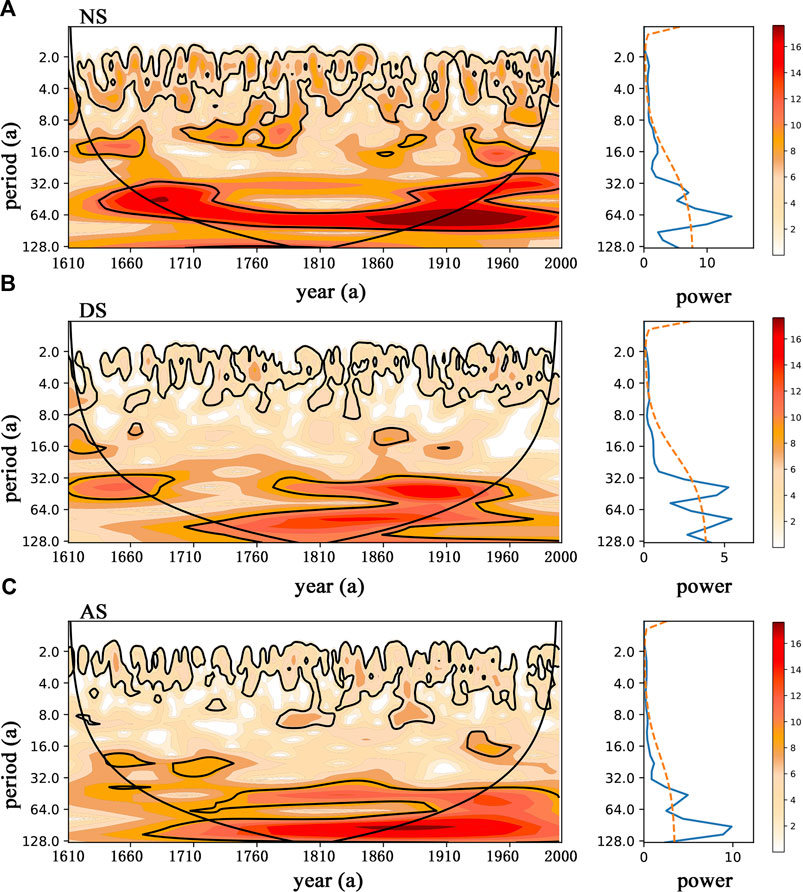
FIGURE 7. Wavelet power spectrum analysis of the composite mean AMOCI in the NS test (A), DS test (B), and AS test (C). The conical lines are wavelet cones, which denote the confidence region. The areas surrounded by the black lines in the wavelet cones are the areas that pass the 95% significance test. The power spectrum is shown on the right, with the dashed line indicating the 95% significance test line.
3.3 Effect of solar forcing
In Section 3.2, on one hand, AMOCI decreased in the three groups during the period from 1800 to 2000 and the decline rate in DS was the largest, followed by the AS test. On the other hand, the AMOCI showed obvious characteristics of two groups of multidecadal cycles, in which the cycle of AMOCI in the AS test was the longest, followed by the DS and NS tests. The AMOC showed an obvious significant response in strength and extended time scale variability to decadal and centennial TSI variations. Since ocean temperature and salinity are key factors influencing the AMOC, we investigated the responses of ocean temperature and salinity.
Figure 8 shows the difference in the ocean temperatures between the DS and NS tests (a–c) and between the AS and NS tests (b–f) at three ocean depths. Panels (a) and (d) show the results at the surface (SST). Panels (b) and (e) show the results at a depth of 300 m. Panels (c) and (f) show the results at a depth of 1,000 m.
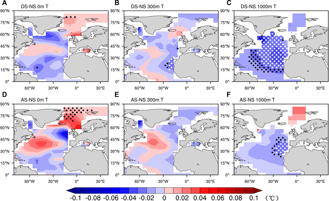
FIGURE 8. Sea temperature differences in the surface layer (A), 300 m depth (B), and 1,000 m depth (C) in DS and NS between 1610 and 2000. (D–F) shows the differences temperature at surface, 300 m, 1000 m depth between AS and NS. The black dotted area is significant at the 95% level for a two-tailed T-test, and the white area is the 99% significance test.
The typical tripolar pattern of the SST in the N.A. region is shown in Figure 8A. The warming SST appears from the polar region to the Greenland–Norway Sea (GNS) with 95% confidence. A significant cooling at a depth of 300 m located on the east side of the Atlantic subtropical gyre was detected, as shown in Figure 8B, which is consistent with Canary cold current flows. Panel (c) shows significant cooling in the whole circulation field in the N.A. at a depth of 1,000 m. In the results showing the difference between AS and NS in Figure 8D, more area with a significant positive response of SST was observed in the GNS.
Figure 9 is similar to Figure 8, but it shows the differences in salinity. Figures 9A, D show a significant negative anomaly in the surface salinity in the Barents Sea (BRS) in the DS and AS tests. The significant westward extension of this negative anomaly was revealed in the DS test.
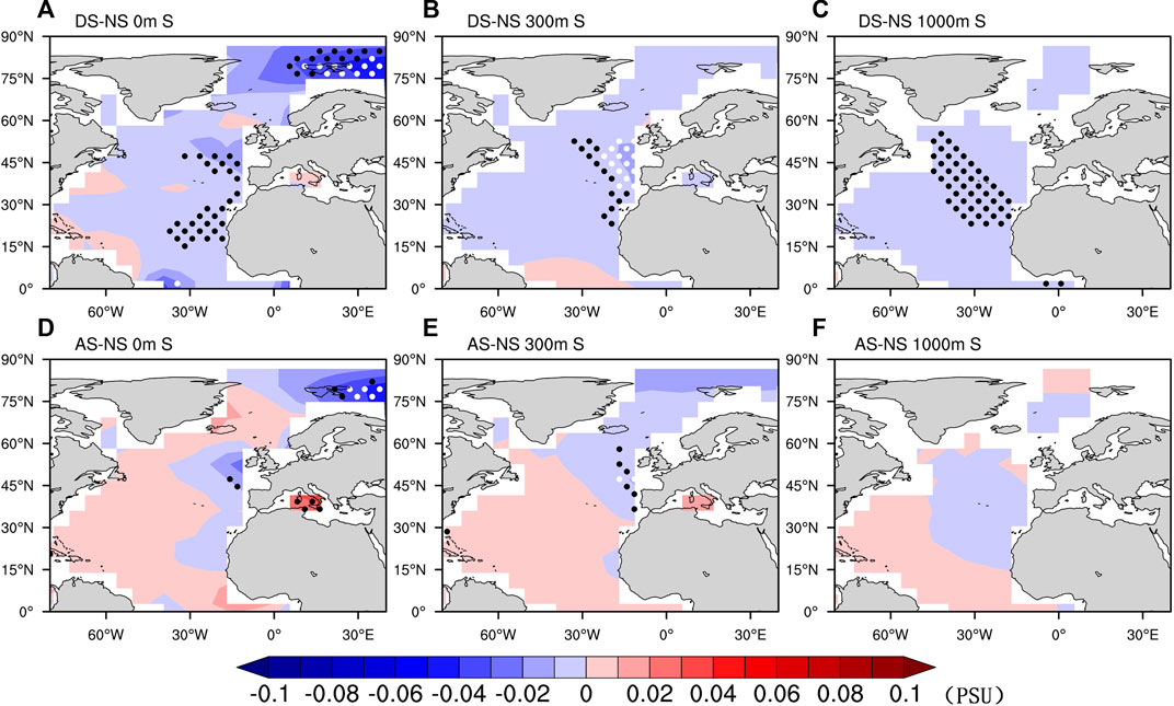
FIGURE 9. Same as Figure 8 but for the difference in salinity.
Figure 10 shows the differences in sea–ice cover (SIC) between the DS and AS tests and the control run (NS). Comparing panels (a) and (b), in the AS test, the full variability in TSI leads to more significant ice melting in the Arctic region.
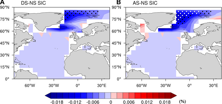
FIGURE 10. ea–ice cover (SIC) difference among DS (A), AS (B), and NS. The black dotted area is significant at the 95% level for a two-tailed T-test, while the white area is significant at the 99% level.
Figure 11 shows the wind stress discrepancy among DS (panel (a)), AS (panel (b)), and NS. With the solar forcing, the wind stress in the Greenland Sea is significantly strengthened. In the DS test, there is a clear southward enhancement of wind stress, which would increase the East Greenland Current (EGC) and transport more melted fresh water from the Arctic to the west subpolar gyre (wSPG). Consequently, the salinity and temperature in the SPG would decline.
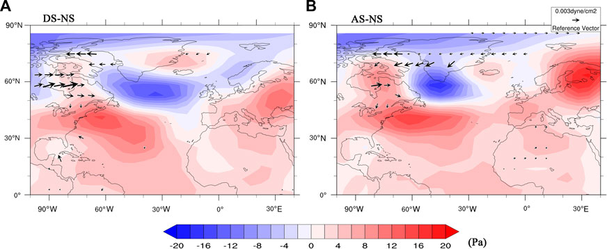
FIGURE 11. Wind stress discrepancy among DS (A), AS (B), and NS. The arrow represents the result with statistical significance at 99%. The contour indicates the difference in surface pressure.
Figure 12 shows the mixed layer depth (MLD) discrepancy among DS (panel (a)), AS (panel (b)), and NS. With solar forcing, the MLD in the wSPG is shallower than that in the NS test. The DS test shows a significant negative response, which is consistent with the intensified EGC shown in Figure 11. This finding could lead to a decline in the AMOC.
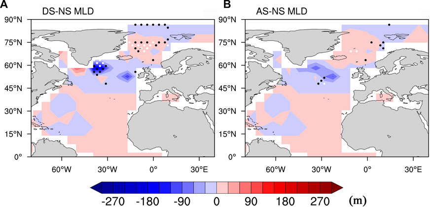
FIGURE 12. Same as Figure 10 but for the difference in MLD.
To understand the accelerated weakening trend of the AMOC since 1800 due to solar forcing, the correlation of SST/sea surface salinity (SSS) with the AMOCI was determined, as shown in Figure 13, in which panels (a–c) show the correlations between the SST and AMOCI, and panels (d–f) show the correlations between the SSS and AMOCI.
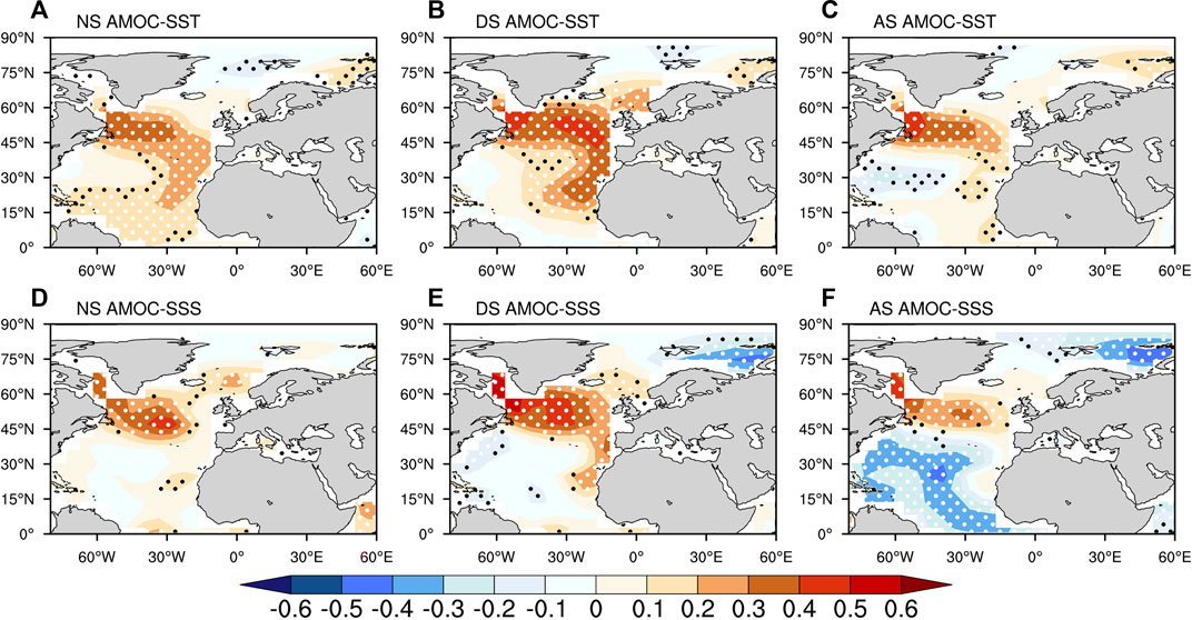
FIGURE 13. Correlation between annual AMOCI and SST (The top panels) and SSS (The bottom panels) in the NS test (A,D), DS test (B,E), and AS test (C,F) from 1800 to 2000. The black dots indicate the 95% significance level for the correlation, while the white indicates the 99% significance level. The contours represent the correlation coefficients.
As shown in Figures 13A, D, with a constant TSI, SST and SSS in the SPG and the Labrador Sea (LAS) have a significant positive correlation with the AMOCI. In the DS and AS tests, the significant negative contribution of SSS in the BRS would be induced by varied TSI, which is shown in panels (e) and (f). The DS test showed more positive contributions to SST and SSS than in the AS test.
Figure 14 reveals the correlation between the TSI of the DS and AS tests and the SST/SSS results. In the DS test, TSI is negatively correlated with SST in the SPG and LAS. TSI was also positively correlated with SSS in the BRS. However, in the AS test, only a positive correlation between TSI and SSS could be found in the BRS, and a weak positive correlation between TSI and SST was detected in SPG and LAS.
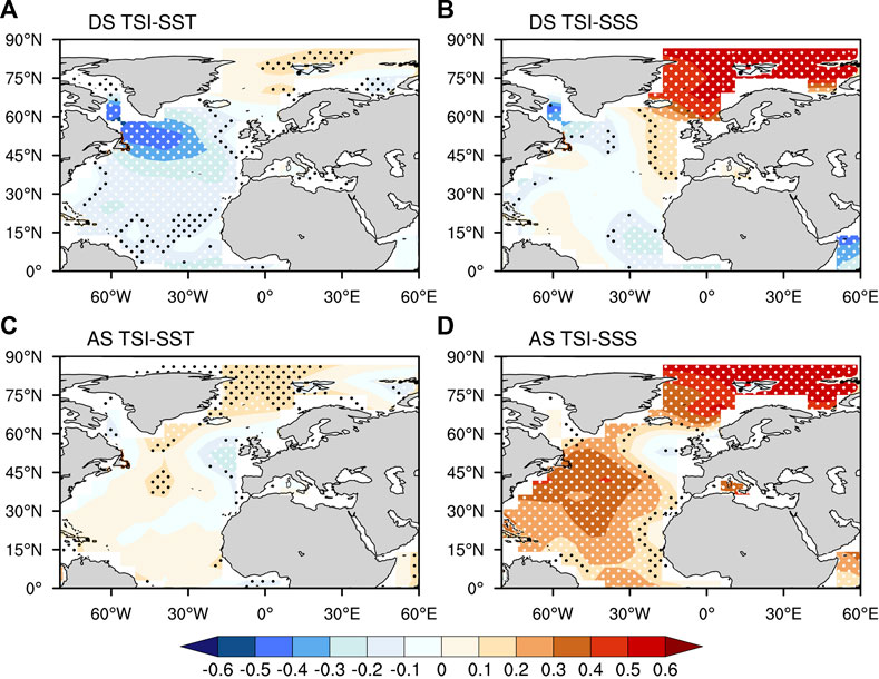
FIGURE 14. Oceanic fields correlated with the annual TSI forcing from 1800 to 2000. (A) SST in the DS test (in °C), (B) SSS in DS (in psu), (C) SST in the AS test, and (D) SSS in AS. The black dots in (A–D) indicate the 95% significance level, while the white dots indicate the 99% significance level. The contours represent correlation coefficients.
By combining the results in Figure 8 with those in Figure 14, the SST in the SPG and the SSS in the BRS may account for the weakening of the AMOC in the DS test. The TSI was negatively correlated with SST in the SPG and positively correlated with SSS in the BRS, which would cause a negative contribution to the AMOC. In the AS test, the negative contribution of the SSS in the BRS to the AMOC could be partly balanced by the positive contribution of the SST in SPG. The Atlantic water heat transport through the BRS Opening and solar heat flux has been proposed to contribute equally to the climate variability in the BRS (Sando et al., 2010). A coupled ice–ocean model simulation by Long and Perrie (2017) revealed that increased lateral heat transport and solar radiation account for the increasing SST in the southern BRS, which is consistent with our simulation.
The branch of Atlantic water transits the BRS, forming BRS Water (BSW) (Harris et al., 1998; Schauer et al., 2002). BSW is entrained in Arctic Intermediate Water (Schauer et al., 1997; Maslowski et al., 2004), which is ultimately exported to the N.A. and in turn contributes to the deeper branch of the AMOC (Aagaard and Woodgate, 2001; Barton et al., 2018). Therefore, SST and SSS in the BRS and SPG were treated as the key factors affecting the AMOC. Figures 15A, B show the regional mean SST and SSS in the BRS, 75°N–90°N, 20–60°E) and Figures 15C, D show those in the Labrador Sea and west SPG (LAS-wSPG, 50°N–70°N, 45°W–65°W) based on the NS (gray line), DS (red line), and AS (blue line) tests. The dashed line is the fitting curve of the results after 1800.
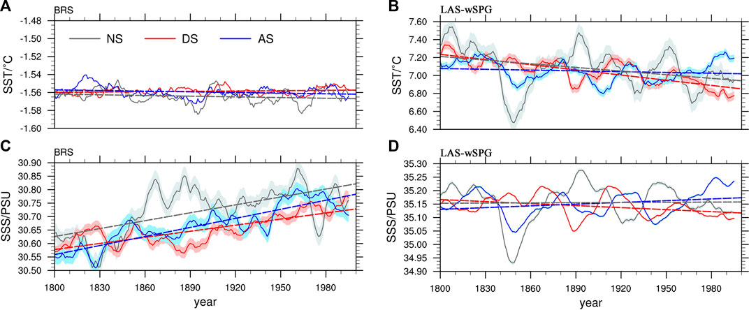
FIGURE 15. Mean values (11-year smoothed) of the sea surface temperature (SST) and sea surface salinity (SSS) in the BRS (75°N–90°N, 20°E−60°E) (A,B) and LAS-wSPG (50°N–70°N, 45°W–65°W) (C,D). Gray line, NS test; red line, DS test; blue line, AS test; dashed lines, fitting curves of the results from 1800 to 2000.
In the BRS, according to all three tests, the long-term trend of SST maintained a very small change and showed continuous increasing trends in SSS. Without the varied TSI forcing, the quantitative values of SST and SSS in the NS test were larger than those in the DS and AS tests. The increasing trend of SSS in the BRS may have contributed to the weakening trend of the AMOC after 1800.
In the LAS-wSPG region, the NS and DS tests showed a decreasing trend in SST. In the DS test, the trend showed a larger decreasing rate than that in the NS test. In the AS test, in the long term, the trend remained nearly constant; even after 1940, the SST showed a continuous increase. For the SSS in LAS-wSPG, the NS and AS tests showed a slight long-term increasing trend. The DS test showed a significant long-term decreasing trend. Thus, in the DS test, the decreased SSS is attributed to the intensified EGC and Greenland ice sheet (GrIS) melting.
Multilinear regression analysis was performed to evaluate the potential effects of the SST and SSS in the BRS and LAS-wSPG. The results are shown in Table 1, in which the SSS in LAS-wSPG accounted for most of the AMOC in all three tests. Compared with the results in Figures 13–15, in both the DS and AS tests with variable TSI, the increased SSS in the BRS led to a weakening of the AMOC. In the DS test, the decreased SSS in LAS-wSPG could strengthen this weakening trend. However, in the AS test, the increased SSS had a positive effect on the AMOC, which partly balanced the negative contribution of the SSS to the BRS.

TABLE 1. Solar forcing response of the AMOCI based on a regression analysis. The regression coefficients (R.C.) for the SST and SSS in the BRS and LAS-wSPG are shown. *95% statistical significance; **99% statistical significance.
4 Discussion and conclusion
Many previous simulations have addressed two kinds of multidecadal variations in AMOC and have reported two main variabilities at 20–30 and 50–70 years, which accounted for the internal interaction of ocean currents or ice–ocean–atmosphere in the N.A. region (Delworth et al., 1993; Timmermann et al., 1998; Ortega et al., 2015). In our simulation, the control simulation of NS reproduced both variabilities. The whole solar forcing in the AS test showed a significantly extended period cycle. The high-frequency part of 30–40 years remained, and a low frequency of 100-year variation appeared due to the centennial variation in TSI, which could contribute to the low frequency (60–100 years) of variability in the AMOC based on the tree ring proxy (Gray et al., 2004).
The DS and AS tests showed that the SPG and BRS are crucial regions and that the SSS in these two regions is the main factor affecting the solar forcing that links to the AMOC. In the DS test, the SSS in SPG dominated the AMOC variability. Although we expected that the variation in GrIS melting due to the solar forcing would dominate the SSS variability in wSPG, the meridional wind was the key factor, which is consistent with other studies, including the study by Li et al. (2021). In the DS and AS tests, the solar forcing led to a significant positive effect on the strength of the southward meridional wind along East Greenland, which controls the EGC intensity. EGC intensity was negatively related to the SSS in SPG and was even considered to account for the phase reversal of a bidecadal ocean mode in the N.A (Escudier et al., 2013). Then, linked by EGC intensity, the decadal variation in TSI was negatively connected to the SSS in SPG. In the BRS, seawater is considered a water source that feeds the AMOC through the Nordic Sea (Lozier et al., 2019). The SIC has been proposed to be negatively related to the AMOC due to “the Barents Sea cooling machine” (øystein Skagseth, 2020), which suggested that the low SIC in the BRS increased the heat loss and weakened the deep thermal convection. The solar forcing in the DS or AS test positively affected the SIC in the BRS, which led to a negative effect on the AMOC due to the Barents Sea cooling machine.
The weakening of the AMOC in recent decades or even in the past few centuries has been reported (Caesar et al., 2018; Collins, 2019); however, this declining trend is controversial (Moat et al., 2020). The origin of the weakening has been attributed to anthropogenic effects (Swingedouw et al., 2022) or natural forcing (Latif et al., 2022). Our work assessed the contribution of solar forcing-modified TSI. With the real TSI in the AS test, the weakening AMOC with a decline rate of −0.41 Sv per century was investigated, which is approximately 24% of the whole AMOC weakening trend assessed by Caesar et al. (2018). Based on the sensitivity tests, the main effect of the TSI on AMOC weakening was attributed to the decadal variation in TSI through its negative effect on salinity in the LAS-wSPG and positive effect on salinity in the BRS. The decline in salinity due to increased freshwater flux from GrIS melting and transportation by strengthened EGC intensity and ice melting water from the LAS was the main contributor to the decline in the AMOC. In addition to TSI variability, which is 0.1%–0.2% of the TSI, solar activity also causes other changes that could directly affect the low atmosphere in the N.A., such as solar irradiance variation in the ultraviolet band (Haigh, 1994), the precipitation flux of energetic particles (Lu et al., 2008), solar wind, and the global electric circuit (Tinsley and Zhou, 2006). These factors could also be the source of the weakening AMOC. For example, solar wind-driven variability in relativistic electron flux could lead to a significant wind stress response in the N.A. region (Mironova et al., 2012; Zhou et al., 2014), and the response of the surface pressure and wind to the fluctuation in the interplanetary magnetic field has been reported (Lam et al., 2014; Zhou et al., 2018; Tinsley et al., 2021). The solar wind-driven global electric circuit has been suggested to lead to a significant atmospheric dynamic response in the N.A. region through electric-cloud microphysics (Tinsley, 2008), which could also contribute to AMOC variability.
This study assessed the effects of different TSI forcings on AMOC multidecadal variability since the Little Ice Age using an Earth System Model with intermediate complexity, PLASIM-GENIE, version 1.0. Although it is a coarse resolution model and the atmospheric part of the model is simplified, the main features of the ocean and atmosphere circulations can be successfully reproduced, including the two multidecadal variabilities in AMOC. According to the simulation results, the effect of GrIS melting through the Labrador Sea on the MLD in the wSPG was also detected.
Data availability statement
The raw data supporting the conclusion of this article will be made available by the authors, without undue reservation.
Author contributions
AY: conceptualization, methodology, software, simulation, data analysis, and writing—original draft; ZZ: data curation and writing—original draft; RZ: visualization; ZX: resources and investigation; LZ: conceptualization, funding acquisition, resources, supervision, and writing—review and editing. All authors contributed to the article and approved the submitted version.
Funding
This work was funded in part by the Strategic Priority Research Program of CAS (Grant No. XBD 41000000) and the National Science Foundation of China (41971020 and 42271027).
Acknowledgments
The authors would like to thank Dr. Philip B. Holden for providing the code for PLASIM-GENIE v1.0.
Conflict of interest
The authors declare that the research was conducted in the absence of any commercial or financial relationships that could be construed as a potential conflict of interest.
Publisher’s note
All claims expressed in this article are solely those of the authors and do not necessarily represent those of their affiliated organizations, or those of the publisher, the editors, and the reviewers. Any product that may be evaluated in this article, or claim that may be made by its manufacturer, is not guaranteed or endorsed by the publisher.
Abbreviations
AMOC, Atlantic meridional overturning circulation; AMOCI, AMOC index; AS, reconstructed whole total solar irradiance forcing test; BRS, Barents Sea; BSW, Barents sea water; DS, decadal varied total solar irradiance forcing test; EGC, East Greenland Current; EMD, empirical mode decomposition; GNS, Greenland–Norway Sea; GrIS, Greenland ice sheet; HadGEM2-ES, Hadley Centre Global Environment Model 2, with Earth System components; IPCC-AR6, the Sixth Assessment Report of the Intergovernmental Panel on Climate Change; LAS, Labrador Sea; LAS-wSPG, Labrador Sea and west subpolar gyre; MLD, mixed layer depth; N.A., North Atlantic; NS, constant total solar irradiance (1,364.5 W/m2) forcing test; PLASIM-GENIE, Earth System model with intermediate complexity used in this research; RAPID, Rapid Climate Change program; SIC, sea–ice cover; SPG, subpolar gyre; SSS, sea surface salinity; SST, sea surface temperature; Sv, Sverdrup, the unit of AMOC. 1 Sv = 1×10⁶ m3/s(−1); TSI, total solar irradiance.
References
Aagaard, K., and Woodgate, R. A. (2001). Some thoughts on the freezing and melting of sea ice and their effects on the ocean. Ocean. Model. 3 (1-2), 127–135. doi:10.1016/S1463-5003(01)00005-1
Andrews, M. B., Knight, J. R., and Gray, L. J. (2015). A simulated lagged response of the North Atlantic Oscillation to the solar cycle over the period 1960-2009. Environ. Res. Lett. 10 (5), 054022. doi:10.1088/1748-9326/10/5/054022
Bagatinsky, V. A., and Diansky, N. A. (2021). Variability of the North Atlantic thermohaline circulation in different phases of the atlantic multidecadal oscillation from ocean objective analyses and reanalyses. Izvestiya. Atmos. Ocean. Phys. 57 (2), 208–219. doi:10.1134/S000143382102002X
Barton, B. I., Lenn, Y., and Lique, C. (2018). Observed atlantification of the Barents Sea causes the polar front to limit the expansion of winter sea ice. J. Phys. Oceanogr. 48 (8), 1849–1866. doi:10.1175/JPO-D-18-0003.1
Caesar, L., Mccarthy, G. D., Thornalley, D., Cahill, N., and Rahmstorf, S. (2021). Current atlantic meridional overturning circulation weakest in last millennium. Nat. Geosci. 14 (3), 118–120. doi:10.1038/s41561-021-00699-z
Caesar, L., Rahmstorf, S., Robinson, A., Feulner, G., and Saba, V. (2018). Observed fingerprint of a weakening Atlantic Ocean overturning circulation. Nature 556 (7700), 191–196. doi:10.1038/s41586-018-0006-5
Cheng, J., Liu, Z., Zhang, S., Liu, W., Dong, L., Liu, P., et al. (2016). Reduced interdecadal variability of atlantic meridional overturning circulation under global warming. Proc. Natl. Acad. Sci. 113 (12), 3175–3178. doi:10.1073/pnas.1519827113
Chylek, P., Folland, C., Frankcombe, L., Dijkstra, H., Lesins, G., and Dubey, M. (2012). Greenland ice core evidence for spatial and temporal variability of the Atlantic Multidecadal Oscillation. Geophys. Res. Lett. 39. doi:10.1029/2012GL051241
Collins, M. M. S. L. (2019). “IPCC special Report on the ocean and cryosphere in a changing climate,” in Chapter 6: Extremes, abrupt changes and managing risks. Reprinted.
de Lavergne, C., Madec, G., Roquet, F., Holmes, R. M., and Mcdougall, T. J. (2017). Abyssal ocean overturning shaped by seafloor distribution. Nature 551 (7679), 181–186. doi:10.1038/nature24472
Delworth, M. L., Syukuro, M., and Ronald, S. (1993). Inter-decadal variations of the thermohaline circulation in a coupled ocean atmosphere model. J. Clim. 6. doi:10.1175/1520-0442(1993)006<1993:IVOTTC>2.0.CO;2
Eby, M., Weaver, A., Alexander, K., Zickfeld, K., Abe-Ouchi, A., Cimatoribus, A., et al. (2013). Historical and idealized climate model experiments: Anintercomparison of Earth system models of intermediate complexity. Clim. Past 9, 1111–1140. doi:10.5194/cp-9-1111-2013
Eddy, J. A. (1976). The maunder minimum. Science 192 (4245), 1189–1202. doi:10.1126/science.192.4245.1189
Escudier, R., Mignot, J., and Swingedouw, D. (2013). A 20-year coupled ocean-sea ice-atmosphere variability mode in the North Atlantic in an AOGCM. Clim. Dyn. 40, 619–636. doi:10.1007/s00382-012-1402-4
Foukal, P., Fröhlich, C., Spruit, H., and Wigley, T. M. L. (2006). Variations in solar luminosity and their effect on the Earth's climate. Nature 443, 161–166. doi:10.1038/nature05072
Goosse, H., and Renssen, H. (2006). Regional response of the climate system to solar forcing: The role of the ocean. Space Sci. Rev. 125 (1-4), 227–235. doi:10.1007/s11214-006-9059-0
Gray, L. J., Anstey, J. A., Kawatani, Y., Lu, H., Osprey, S., and Schenzinger, V. (2018). Surface impacts of the quasi biennial oscillation. Atmos. Chem. Phys. 18 (11), 8227–8247. doi:10.5194/acp-18-8227-2018
Gray, L. J., Beer, J., Geller, M., Haigh, J. D., Lockwood, M., Matthes, K., et al. (2010). Solar influences on climate. Rev. Geophys. 48. doi:10.1029/2009RG000282
Gray, L. J., Rumbold, S. T., and Shine, K. P. (2009). Stratospheric temperature and radiative forcing response to 11-year solar cycle changes in irradiance and ozone. J. Atmos. Sci. 66 (8), 2402–2417. doi:10.1175/2009JAS2866.1
Gray, L. J., Scaife, A. A., Mitchell, D. M., Osprey, S., Ineson, S., Hardiman, S., et al. (2013). A lagged response to the 11 year solar cycle in observed winter Atlantic/European weather patterns. J. Geophys. Res. Atmos. 118 (24), 13,405–13,420. doi:10.1002/2013JD020062
Gray, L. J., Woollings, T. J., Andrews, M., and Knight, J. (2016). Eleven-year solar cycle signal in the NAO and Atlantic/European blocking. Q. J. R. Meteorological Soc. 142 (698), 1890–1903. doi:10.1002/qj.2782
Gray, S. T., Graumlich, L. J., Betancourt, J. L., and Pederson, G. T. (2004). A tree-ring based reconstruction of the atlantic multidecadal oscillation since 1567 A.D. Reconstructed atlantic multidecadal oscillation. Geophys. Res. Lett. 31. doi:10.1029/2004GL019932
Gregory, J. M., Dixon, K. W., Stouffer, R. J., Weaver, A. J., Driesschaert, E., Eby, M., et al. (2005). A model intercomparison of changes in the Atlantic thermohaline circulation in response to increasing atmospheric CO2 concentration. Geophys. Res. Lett. 32 (12), n/a. doi:10.1029/2005gl023209
Haigh, J. D. (1996). The impact of solar variability on climate. Science 272 (5264), 981–984. doi:10.1126/science.272.5264.981
Haigh, J. D. (1994). The role of stratospheric ozone in modulating the solar radiative forcing of climate. Nature 370, 544–546. doi:10.1038/370544a0
Harris, C. L., Plueddemann, A. J., and Gawarkiewicz, G. G. (1998). Water mass distribution and polar front structure in the Western Barents Sea. J. Geophys. Research-Oceans 103 (C2), 2905–2917. doi:10.1029/97JC02790
Holden, P. B., Edwards, N. R., Fraedrich, K., Kirk, E., Lunkeit, F., and Zhu, X. (2016). PLASIM–GENIE v1.0: A new intermediate complexity AOGCM. Geosci. Model Dev. 9 (9), 3347–3361. doi:10.5194/gmd-9-3347-2016
Holliday, N. P., Bersch, M., Berx, B., Chafik, L., Cunningham, S., Florindo-Lopez, C., et al. (2020). Ocean circulation causes the largest freshening event for 120 years in eastern subpolar North Atlantic. Nat. Commun. 11 (1), 585. doi:10.1038/s41467-020-14474-y
Huang, B., Zhu, J., and Yang, H. (2014). Mechanisms of atlantic meridional overturning circulation(AMOC)variability in a coupled ocean – atmosphere GCM. Adv. Atmos. Sci. 31, 241–251. doi:10.1007/s00376-013-3021-3
Huck, T., Vallis, G. K., and de Verdiere, A. C. (2001). On the robustness of the interdecadal modes of the thermohaline circulation. J. Clim. 14 (5), 940–963. doi:10.1175/1520-0442(2001)014<0940:OTROTI>2.0.CO;2
Ineson, S., Scaife, A. A., Knight, J. R., Manners, J. C., Dunstone, N. J., Gray, L. J., et al. (2011). Solar forcing of winter climate variability in the Northern Hemisphere. Nat. Geosci. 4 (11), 753–757. doi:10.1038/NGEO1282
Jackson, L. C., Roberts, M. J., Hewitt, H. T., Iovino, D., Koenigk, T., Meccia, V. L., et al. (2020). Impact of ocean resolution and mean state on the rate of AMOC weakening. Clim. Dyn. 55 (7-8), 1711–1732. doi:10.1007/s00382-020-05345-9
Jiang, Z., Liu, Z., Zhang, X., Eisenman, I., and Liu, W. (2014). Linear weakening of the AMOC in response to receding glacial ice sheets in CCSM3. Geo. Res. Lett. 41, 6252–6258. doi:10.1002/2014GL060891
Kanzow, T., Cunningham, S. A., Johns, W. E., Hirschi, J., Marotzke, J., Baringer, M. O., et al. (2010). Seasonal variability of the atlantic meridional overturning circulation at 26.5°N. J. Clim. 23 (21), 5678–5698. doi:10.1175/2010JCLI3389.1
Kuroda, Y., Kodera, K., Yoshida, K., Yukimoto, S., and Gray, L. (2022). Influence of the solar cycle on the North Atlantic oscillation. J. Geophys. Research-Atmospheres 127 (1). doi:10.1029/2021JD035519
Lam, M. M., Chisham, G., and Freeman, M. P. (2014). Solar wind-driven geopotential height anomalies originate in the Antarctic lower troposphere. Geophys. Res. Lett. 41, 6509–6514. doi:10.1002/2014GL061421
Latif, M., Sun, J., Visbeck, M., and Bordbar, H. (2022). Natural variability has dominated atlantic meridional overturning circulation since 1900. Nat. Clim. Chang. 12, 455–460. doi:10.1038/s41558-022-01342-4
Lean, J. L. (2010). Cycles and trends in solar irradiance and climate. Wiley Interdiscip. Reviews-Climate Change 1 (1), 111–122. doi:10.1002/wcc.18
Lee, S. K., and Wang, C. Z. (2010). Delayed advective oscillation of the atlantic thermohaline circulation. J. Clim. 23 (5), 1254–1261. doi:10.1175/2009JCLI3339.1
Lenton, T. M., Marsh, R., Price, A. R., Lunt, D. J., Aksenov, Y., Annan, J. D., et al. (2007). Effects of atmospheric dynamics and ocean resolution on bi-stability of the thermohaline circulation examined using the Grid ENabled Integrated Earth system modelling (GENIE) framework. Clim. Dyn. 29 (6), 591–613. doi:10.1007/s00382-007-0254-9
Li Dongling, S. L. L. Y. (2016). The influence of the meso-late Holocene cold water mass on disko bay, west Greenland. Oceanol. Limnologia Sinica 47 (06), 1126–1139. doi:10.11693/hyhz20160500101
Li, F., Lozier, M. S., Bacon, S., Bower, A. S., Cunningham, S. A., de Jong, M. F., et al. (2021). Subpolar North atlantic Western boundary density anomalies and the meridional overturning circulation. Nat. Commun. 12, 3002. doi:10.1038/s41467-021-23350-2
Lin, P., Yu, Z., Lü, J., Ding, M., Hu, A., and Liu, H. (2019). Two regimes of atlantic multidecadal oscillation: Cross-basin dependent or atlantic-intrinsic. Sci. Bull. 64 (3), 198–204. doi:10.1016/j.scib.2018.12.027
Liu Jing, S. L. L. Y. (2014). “Middle-late Holocene diatom assemblages and their paleoenvironmental evolution in West Greenland,” in Acta micropalaeontologica sinica. CNKI:SUN:WSGT.0.2014-02-001.
Liu, J., Wang, B., Cane, M. A., Yim, S. Y., and Lee, J. Y. (2013). Divergent global precipitation changes induced by natural versus anthropogenic forcing. Nature 493 (7434), 656–659. doi:10.1038/nature11784
Long, Z., and Perrie, W. (2017). Changes in ocean temperature in the Barents Sea in the twenty-first century. J. Clim. 30 (15), 5901–5921. doi:10.1175/JCLI-D-16-0415.1
Lourantou, A., Chappellaz, J., Barnola, J., Masson-Delmotte, V., and Raynaud, D. (2010). Changes in atmospheric CO2 and its carbon isotopic ratio during the penultimate deglaciation. Quat. Sci. Rev. 29, 1983–1992. doi:10.1016/j.quascirev.2010.05.002
Lozier, M. S., Li, F., Bacon, S., Bahr, F., Bower, A. S., Cunningham, S. A., et al. (2019). A sea change in our view of overturning in the subpolar North Atlantic. Science 363 (6426), 516–521. doi:10.1126/science.aau6592
Lu, H., Clilverd, M., Seppala, A., and Hood, L. (2008). Geomagnetic perturbations on stratospheric circulation in late winter and spring. J. Geophys. Res. 113, D16106. doi:10.1029/2007JD008915
Lynch-Stieglitz, J. (2017). The atlantic meridional overturning circulation and abrupt climate change. Annu. Rev. Mar. Sci. 9 (1), 83–104. doi:10.1146/annurev-marine-010816-060415
Mann, M. E., Steinman, B. A., Brouillette, D. J., and Miller, S. K. (2021). Multidecadal climate oscillations during the past millennium driven by volcanic forcing. Science 371 (6533), 1014–1019. doi:10.1126/science.abc5810
Mann, M. E., Zhang, Z. H., Rutherford, S., Bradley, R. S., Hughes, M. K., Shindell, D., et al. (2009). Global signatures and dynamical origins of the Little ice Age and medieval climate anomaly. Science 326 (5957), 1256–1260. doi:10.1126/science.1177303
Marsh, R., Yool, A., Lenton, T. M., Gulamati, M. Y., Edwards, N. R., Shepherd, J. G., et al. (2004). Bistability of the thermohaline circulation identified through comprehensive 2-parameter sweeps of an efficient climate model. Clim. Dyn. 23 (7-8), 761–777. doi:10.1007/s00382-004-0474-1
Maslowski, W., Marble, D., Walczowski, W., Schauer, U., Clement, J. L., and Semtner, A. J. (2004). On climatological mass, heat, and salt transports through the Barents Sea and Fram Strait from a pan-Arctic coupled ice-ocean model simulation. J. Geophys. Research-Oceans 109 (C3). doi:10.1029/2001JC001039
Masson-Delmotte, V. P. Z. A. (2021). The physical science Basis.Contribution of working group I to the Sixth assessment Report of the intergovernmental panel on climate change: IPCC, climate change 2021. Reprinted.
Menary, M. B., Roberts, C. D., Palmer, M. D., Halloran, P. R., Jackson, L., Wood, R. A., et al. (2013). Mechanisms of aerosol-forced AMOC variability in a state of the art climate model. J. Geophys. Research-Oceans 118 (4), 2087–2096. doi:10.1002/jgrc.20178
Menary, M. B., and Scaife, A. A. (2014). Naturally forced multidecadal variability of the Atlantic meridional overturning circulation. Clim. Dyn. 42 (5-6), 1347–1362. doi:10.1007/s00382-013-2028-x
Mironova, I., Tinsley, B. A., and Zhou, L. (2012). The links between atmospheric vorticity, radiation belt electrons, and the solar wind. Adv. Space Res. 50. doi:10.1016/j.asr.2011.03.043
Moat, B. I., Smeed, D. A., Frajka-Williams, E., Desbruyères, D. G., Beaulieu, C., Johns, W. E., et al. (2020). Pending recovery in the strength of the meridional overturning circulation at 26° N. Ocean Sci. 16, 863–874. doi:10.5194/os-16-863-2020
Muthers, S., Raible, C. C., Rozanov, E., and Stocker, T. F. (2016). Response of the AMOC to reduced solar radiation – The modulating role of atmospheric chemistry. Earth Syst. Dyn. 7 (4), 877–892. doi:10.5194/esd-7-877-2016
Negre, C., Zahn, R., Thomas, A. L., Masque, P., Henderson, G. M., Martinez-Mendez, G., et al. (2010). Reversed flow of atlantic deep water during the last glacial maximum. Nature 468 (7320), 84–88. doi:10.1038/nature09508
Ortega, P., Mignot, J., Swingedouw, D., Sevellec, F., and Guilyardi, E. (2015). Reconciling two alternative mechanisms behind bi-decadal variability in the North Atlantic. Prog. Oceanogr. 137, 237–249. doi:10.1016/j.pocean.2015.06.009
øystein Skagseth, T. E. M. Å., Eldevik, T., Årthun, M., Asbjørnsen, H., Lien, V. S., and Smedsrud, L. H. (2020). Reduced efficiency of the Barents Sea cooling machine. Nat. Clim. Change 10, 661–666. doi:10.1038/s41558-020-0772-6
Park, W., and Latif, M. (2012). Atlantic Meridional Overturning Circulation response to idealized external forcing. Clim. Dyn. 39 (7-8), 1709–1726. doi:10.1007/s00382-011-1212-0
Ran Lihua, J. H. K. K. (2008). Paleomarine environmental records since the middle Holocene in the northern North Atlantic. Mar. Sci. Bull (05), 39–46+7. doi:10.3969/j.issn.1001-6392.2008.05.007
Sando, A. B., Nilsen, J. E. O., Gao, Y., and Lohmann, K. (2010). Importance of heat transport and local air-sea heat fluxes for Barents Sea climate variability. J. Geophys. Research-Oceans 115, C07013. doi:10.1029/2009JC005884
Scaife, A. A., Ineson, S., Knight, J. R., Gray, L., Kodera, K., and Smith, D. M. (2013). A mechanism for lagged North Atlantic climate response to solar variability. Geophys. Res. Lett. 40 (2), 434–439. doi:10.1002/grl.50099
Schauer, U., Loeng, H., Rudels, B., Ozhigin, V. K., and Dieck, W. (2002). Atlantic water flow through the Barents and kara seas. Deep-Sea Res. Part Oceanogr. Res. Pap. 49 (12), 2281–2298. doi:10.1016/S0967-0637(02)00125-5
Schauer, U., Muench, R. D., Rudels, B., and Timokhov, L. (1997). Impact of eastern arctic shelf waters on the Nansen Basin intermediate layers. J. Geophys. Research-Oceans 102 (C2), 3371–3382. doi:10.1029/96JC03366
Sedlacek, J., and Mysak, L. A. (2009). A model study of the Little ice Age and beyond: Changes in ocean heat content, hydrography and circulation since 1500. Clim. Dyn. 33 (4), 461–475. doi:10.1007/s00382-008-0503-6
Shindell, D. T., Schmidt, G. A., Mann, M. E., Rind, D., and Waple, A. (2001). Solar forcing of regional climate change during the maunder minimum. Science 294 (5549), 2149–2152. doi:10.1126/science.1064363
Sjolte, J., Sturm, C., Adolphi, F., Vinther, B. M., Werner, M., Lohmann, G., et al. (2018). Solar and volcanic forcing of North Atlantic climate inferred from a process-based reconstruction. Clim. Past 14 (8), 1179–1194. doi:10.5194/cp-14-1179-2018
Sutton, R. T., and Hodson, D. (2005). Atlantic Ocean forcing of North American and European summer climate. Science 309 (5731), 115–118. doi:10.1126/science.1109496
Swingedouw, D., Houssais, M. N., Herbaut, C., Blaizot, A. C., Devilliers, M., and Deshayes, J. (2022). AMOC recent and future trends: A crucial role for oceanic resolution and Greenland melting? Front. Clim. 4, 838310–838318. doi:10.3389/fclim.2022.838310
Swingedouw, D., Terray, L., Cassou, C., Voldoire, A., Salas-Melia, D., and Servonnat, J. (2011). Natural forcing of climate during the last millennium: Fingerprint of solar variability. Clim. Dyn. 36 (7-8), 1349–1364. doi:10.1007/s00382-010-0803-5
Timmermann, A., Latif, M., Voss, R., and Grotzner, A. (1998). Northern hemispheric interdecadal variability: A coupled air-sea mode. J. Clim. 11 (8), 1906–1931. doi:10.1175/1520-0442-11.8.1906
Ting, M. F., Kushnir, Y., Seager, R., and Li, C. H. (2011). Robust features of Atlantic multi-decadal variability and its climate impacts. Geophys. Res. Lett. 38. doi:10.1029/2011GL048712
Tinsley, B. A. (2008). The global atmospheric electric circuit and its effects on cloud microphysics. Rep. Prog. Phys. 71, 066801. doi:10.1088/0034-4885/71/6/066801
Tinsley, B. A., and Zhou, L. (2006). Initial results of a global circuit model with variable stratospheric and tropospheric aerosols. J. Geophys. Research-Atmospheres 111 (D16), D16205. doi:10.1029/2005JD006988
Tinsley, B. A., Zhou, L., Wang, L., and Zhang, L. (2021). Seasonal and solar wind sector duration influences on the correlation of high latitude clouds with ionospheric potential. J. Geophys. Res. Atmos. 126. doi:10.1029/2020JD034201
Wang, Y. J., Cheng, H., Edwards, R. L., He, Y. Q., Kong, X. G., An, Z. S., et al. (2005). The Holocene asian monsoon: Links to solar changes and North Atlantic climate. Science 308 (5723), 854–857. doi:10.1126/science.1106296
Xu, H. Y., Miyahara, H., Horiuchi, K., Matsuzaki, H., Sun, H. L., Luo, W. J., et al. (2019). High-resolution records of Be-10 in endogenic travertine from baishuitai, China: A new proxy record of annual solar activity? Quat. Sci. Rev. 216, 34–46. doi:10.1016/j.quascirev.2019.05.012
Yu Lei, G. Y. W. H. (2009). Response and mechanism of Atlantic meridional overturning circulation under high latitude freshwater forcing enhancement. Chin. J. Atmos. Sci 33 (01), 179–196. CNKI:SUN:DQXK.0.2009-01-015.
Yu, L., Gao, Y., Wang, H., Guo, D., and Li, S. (2010). The responses of east Asian summer monsoon to the North Atlantic meridional overturning circulation in an enhanced freshwater input simulation. Chin. Sci. Bull. 54, 4724–4732. doi:10.1007/s11434-009-0720-3
Zhang, R. (2008). Coherent surface-subsurface fingerprint of the Atlantic meridional overturning circulation. Geophys. Res. Lett. 35 (20), L20705. doi:10.1029/2008GL035463
Zhang, R., and Delworth, T. L. (2006). Impact of Atlantic multidecadal oscillations on India/Sahel rainfall and Atlantic hurricanes. Geophys. Res. Lett. 33 (17), L17712. doi:10.1029/2006GL026267
Zhao Yun, S. L. L. Y. (2015). “Paleo-environmental records based on diatoms since the last deglaciation of the northern shelf of Iceland,” in Marine geology and quaternary geology. CNKI:SUN:HYDZ.0.2015-03-014.
Zhou, L. M., Tinsley, B. A., and Huang, J. (2014). Effects on winter circulation of short and long term solar wind changes. Adv. Space Res. 54, 2478–2490. doi:10.1016/j.asr.2013.09.017
Zhou, L., Tinsley, B. A., Wang, L., and Burns, G. (2018). The zonal-mean and regional tropospheric pressure responses to changes in ionospheric potential. J. Atmos. Solar-Terrestrial Phys. 171, 111–118. doi:10.1016/j.jastp.2017.07.010
Zorita, E., Von Storch, H., Gonzalez-Rouco, F. J., Cubasch, U., Luterbacher, J., Legutke, S., et al. (2004). Climate evolution in the last five centuries simulated by an atmosphere-ocean model: Global temperatures, the North Atlantic oscillation and the late maunder minimum. Meteorol. Z. 13 (4), 271–289. doi:10.1127/0941-2948/2004/0013-0271
Keywords: solar forcing, AMOC, multidecadal variability, sensitivity test, period
Citation: Ye A, Zhu Z, Zhang R, Xiao Z and Zhou L (2023) Influence of solar forcing on multidecadal variability in the Atlantic meridional overturning circulation (AMOC). Front. Earth Sci. 11:1165386. doi: 10.3389/feart.2023.1165386
Received: 14 February 2023; Accepted: 02 May 2023;
Published: 19 May 2023.
Edited by:
Nicola Scafetta, University of Naples Federico II, ItalyReviewed by:
Anthony Lupo, University of Missouri, United StatesAna G. Elias, Universidad Nacional de Tucumán, Argentina
Copyright © 2023 Ye, Zhu, Zhang, Xiao and Zhou. This is an open-access article distributed under the terms of the Creative Commons Attribution License (CC BY). The use, distribution or reproduction in other forums is permitted, provided the original author(s) and the copyright owner(s) are credited and that the original publication in this journal is cited, in accordance with accepted academic practice. No use, distribution or reproduction is permitted which does not comply with these terms.
*Correspondence: Limin Zhou, bG16aG91QGdlby5lY251LmVkdS5jbg==