Physical quantity characteristics of severe aircraft turbulence near convective clouds over Australia

Using FY–2G satellite data, Aircraft Meteorological Data Relay (AMDAR) downlink data, and the fifth generation European Centre for Medium–Range Weather Forecasts (ECMWF) atmospheric reanalysis of the global climate (ERA5) dataset, we analyzed the circulation, thermal, and dynamic characteristics of the convective aircraft turbulence over Australia in the Southern Hemisphere. The results show that the near-convective clouds turbulence (NCCT) in the Southern Hemisphere mostly occurred in front of deep warm high–pressure ridges in mid–latitude regions and on the left side of the axis of the subtropical westerly jet stream. The isotherms in this area were relatively dense (i.e., large gradients), and the wind speed was high, with strong horizontal and/or vertical cyclonic wind shear. In addition, the NCCT usually occurred near the zero–divergence or zero–vorticity line and in areas with large vertical wind speed gradients. There were also strong vertical and horizontal wind shears in this area, which could easily trigger severe turbulence. Furthermore, the NCCT in the Southern Hemisphere mostly occurred at the intersection of cold and warm temperature advections (i.e., near the zero–temperature advection line), and the turbulence point was located near the high–altitude frontal zone where there was a strong gradient of cold and warm advections. There was temperature inversion with pseudo–equivalent potential temperatures in the middle and lower troposphere on the warmer side of the turbulence point. The unstable stratification of cold air at the top and warm air at the bottom was conducive to triggering convection from the ground, forming strong convective clouds, and causing severe turbulence.

1 Introduction

Aircraft turbulence is a serious threat to flight safety. Statistics show that 30% of flight accidents can be attributed to meteorological conditions, aircraft turbulence and jet streams account for 6% of the meteorological factors (Williams and Joshi, 2013; Mazon et al., 2018). According to the National Aeronautics and Space Administration (NASA) Weather Accident Prevention Project, airlines incur millions of dollars of economic loss each year due to turbulence, especially the severe aircraft turbulence which can even cause casualties (Sharman et al., 2006; Liao and Xiong, 2010; Prosser et al., 2023). Therefore, it is essential to study the severe aircraft turbulence.

Numerous studies have been conducted on aircraft turbulence in recent decades (Wang, 2006; Huang et al., 2010; Kim et al., 2011; Prosser et al., 2023). A general conclusion is that aircraft turbulence is directly caused by airflow disturbance, and the occurrence and intensity of aircraft turbulence are closely related to meteorological conditions (Kim and Chun, 2016). The airflow disturbance which can trigger the aircraft turbulence usually occurs near the upper jet stream area and the frontal zone, the isotherm dense zone near the high-pressure ridge and the upper trough, and the cumulus clouds area (Kim et al., 2011; Lane et al., 2012). According to the specific meteorological conditions, turbulence can be divided into five types: frontal turbulence, terrain turbulence or mountain wave turbulence, jet stream turbulence, clear–air turbulence, and convective turbulence (Lane et al., 2012; Meneguz et al., 2016; Bramberger et al., 2020; Sharman and Bernstein, 2022).

Many studies have focused on the characteristics and mechanism of these five types of aircraft turbulence. Richardson derived equations based on atmospheric motion principles that reflect the atmospheric conditions during aircraft turbulence, and introduced the Richardson number as a metric to characterize the strength of aircraft turbulence (Wang, 2006; Huang et al., 2010). Other studies have explored the relationship between vertical wind shear, frontogenesis function, and the intensity of turbulence, leading to the development of forecast indices for clear-air turbulence and frontal turbulence (Colson and Panofsky, 1965; Ellrod and Knox, 2010). Additionally, some research has emphasized the importance of thermal and dynamic conditions during aircraft turbulence events, highlighting that the occurrence of aircraft turbulence is caused by the vertical motion of the temperature advection through the edge of the dense isotherm near the upper jet stream (Zhu, 1997). And flying over high altitude plateau routes, the effect of terrain on aircraft turbulence is crucial. A series of studies have revealed the physical mechanism of aircraft turbulence during flight in atmospheric turbulence on the lee side of mountains. The breaking of mountain gravity waves generated by airflow over mountains can also lead to strong downslope winds, lee rotor circulation, and low-level turbulence on the lee side of the mountains, causing severe aircraft turbulence (Li and Huang, 2008; Bramberger et al., 2020). At the same time, meteorologists began focusing on the connection between gravity waves and aircraft turbulence. Research revealed that under stable atmospheric wave conditions, minor wind shear can trigger gravity waves; however, as wind shear increases, stable gravity waves can quickly transition to instability, eventually evolving into atmospheric turbulence that affects aircraft flight (Wang and Zhu, 2001). Furthermore, other studies have confirmed that instability in gravity waves near the tropopause can induce aircraft turbulence in the vicinity of the tropopause (Wang, 2006; Kim and Chun, 2016).

Numerous factors (e.g., jet streams, wind shear, upper-level lows, mountain waves, fronts, etc.) contribute to turbulence, impacting the safety of flight, thus the convective clouds are one of the most important, and convective turbulence is mostly severe and can easily cause casualties and damage to an aircraft (Lane et al., 2012). Convectively induced turbulence is commonly observed in convective clouds; the vertical motion associated with convective processes, such as updrafts and downdrafts, creates varying wind speeds and directions within the cloud. These rapid changes in wind patterns lead to turbulent airflow, which can result in hazardous conditions for aircraft flying through or near convective clouds (Lane et al., 2012; Meneguz et al., 2016). Additionally, specific cloud features like mammatus and anvil regions further contribute to the development of turbulence within convective systems. For instance, a Boeing 777 flying from Washington, D.C. to Los Angeles encountered severe turbulence near a convective cloud system over Missouri on 20 July 2010; the aircraft was diverted to Denver to treat 17 passengers and 4 injured crew members (Lane et al., 2012). For these turbulence processes, avoidance of cloudy air through visual identification or remote sensing with radar and satellite imagery is usually effective (Schultz et al., 2006).

Turbulence generated outside of convective clouds but ultimately caused by convective clouds is also an important factor affecting flight safety that has been appreciated for some time. Because this near-convective clouds turbulence (NCCT) is invisible to pilots and cannot be detected by ground-based radar and standard onboard, although NCCT is usually weaker than turbulence inside convective cores, it is arguably more dangerous (Schultz et al., 2006; Lane et al., 2012). Because the outflow induced by convection is usually stronger and lasts for a long time, an anticyclone can change the wind speed tens of kilometers away by 20–40 m·s^–1, increasing the vertical wind shear and causing aircraft turbulence (Ellrod and Knox, 2010; Yoshimura et al., 2022). Moreover, since the positions of the updraft and downdraft airflow may differ from the positions indicated by radar, many aircraft can be affected by abnormal vertical and horizontal gusts near convective clouds (Trier and Sharman, 2016). Similarly, Lane et al. (2006) have indicated that gravity waves generated by convection are a significant factor contributing to NCCT, ultimately playing a role in the turbulent processes that occur away from the core of the convective cell. For example, because the signal of a large–scale mesoscale strong convective system over southern Missouri in the United States was not displayed on the radar echo, although it avoided the center of the strong convection, a flight at an altitude of 40,000 feet above St. Louis went through severe turbulence at the edge of convective clouds. At present, relatively little is known about the meteorological environment, large-scale circulation features, thermal and dynamic characteristics of near-convective cloud turbulence, especially in the southern hemisphere which has the specific coastal and terrestrial distribution characteristics. Previous studies have shown that further warming of the Southern Ocean throughout the 21st century and the wind-evaporation feedback in the tropical southeastern Indian Ocean can sustain enhanced precipitation and anomalous convection near the Australia (Sekizawa et al., 2018; Cai et al., 2023). Thus, the near-convective clouds turbulence will be likely to increase significantly as the number of the Southern Hemisphere flights increases in the future.

Therefore, an in–depth and detailed analysis of the large-scale circulation, thermal and dynamic characteristics of near convective clouds is critical for further understanding the causes of near-convective clouds turbulence. In this study, based on the typical events of aircraft turbulence in winter over Australia, this article explored the large–scale circulation that caused convective turbulence over Australia. By analyzing such variables as the vertical speed, divergence and vorticity, vertical and horizontal wind shear, temperature advection, and pseudo–equivalent potential temperature, the thermal and dynamic characteristics of aircraft turbulence near convective clouds were quantified.

2 Data and methods

2.1 Data

The data used in this article include 1) hourly mean equivalent black–body temperature products (TBB) of FY–2G satellite in 9,210 format provided by the National Meteorological Information Center (NMIC) of China Meteorological Administration (CMA) at 0200 UTC 5 December 0000 and 0100 UTC 9 December, and 2300 UTC 30 December 2016 (http://data.cma.cn/; only available in Chinese) (Wen et al., 2019); 2) Aircraft Meteorological Data Relay (AMDAR) data provided by the International Civil Aviation Organization and the World Meteorological Organization, which includes information such as time, latitude and longitude, flight altitude, wind direction, wind speed, Derived Equivalent Vertical Gust (DEVG), and Eddy Dissipation Rate (EDR), covering the period from 1 December to 31 December 2016 (Sherman, 1985; Kim et al., 2020; Cai et al., 2023); 3) The European Centre for Medium–Range Weather Forecasts (ECMWF) ERA5 hourly reanalysis data during 1–31 December 2016 with a spatial resolution of 0.25 × 0.25, including specific humidity (g·g⁻¹), zonal and meridional wind (m·s⁻¹), geopotential height (gpm), and surface air temperature (K), etc (Lee et al., 2023).

2.2 Methods

As mentioned above, the near-convective clouds turbulence (NCCT) is closely related to wind shear (Schultz et al., 2006). Localized weather phenomenon, wind shear, can be categorized into three types: 1) vertical wind shear, characterized by changes in horizontal wind speed and/or direction with altitude, 2) horizontal wind shear, which involves changes in horizontal wind speed and/or direction within horizontal space, and 3) downdrafts (microbursts), representing variations in vertical wind speed in horizontal space. As a result, this study aims to diagnose and analyze the characteristics of vertical wind shear, horizontal wind shear, and vertical velocity during the NCCT events, which will help to understand the causes of NCCT.

The vertical wind shear (hereafter referred as vws) has been found to play an important role in the occurrence of aircraft turbulence, so vws is calculated here to examine its effect on near-convective clouds turbulence (Ellrod and Knox, 2010; Prosser et al., 2023). Previous studies have defined the vertical wind shear vector in different ways, and the calculation method of vws used in this study is the widely adopted method internationally (Palmer and Barnes, 2002; Yu et al., 2010), which utilises the vector difference of the regional average wind at 850 hPa and 200 hPa levels to represent the vws. The calculation formula is as follows:

$\mathit{v}\mathit{w}\mathit{s}=\sqrt{{\left({\mathit{u}}_{\mathbf{200}}-{\mathit{u}}_{\mathbf{850}}\right)}^{\mathbf{2}}+{\left({\mathit{v}}_{\mathbf{200}}-{\mathit{v}}_{\mathbf{850}}\right)}^{\mathbf{2}}}.(1)$

where vws (vertical wind shear) represents the change (with altitude) in the speed and/or direction of horizontal wind component; u₂₀₀ and u₈₅₀ are the zonal wind at 200 hPa and 850 hPa levels respectively; and v₂₀₀ and v₈₅₀ are the meridional wind at 200 hPa and 850 hPa levels respectively. Vertical wind shear is considered an important meteorological parameter that has a significant impact on the development and intensity of weather phenomena. This expression can quantify the differences in wind speed at different heights and assess the vertical variation of wind field (Yu et al., 2010). It is important to note that the vertical wind shear here represents the vertical shear of the horizontal wind, not the shear of the vertical wind component.

In order to compare with the results of vertical wind shear calculated in Eq. 1, this study also use another method to calculate vertical wind shear (hereafter referred as vws2), that is, by calculating the vertical derivative of flight height (Kaluza et al., 2022; Rodriguez et al., 2023), to characterize the vertical shear of horizontal wind

$\mathit{v}\mathit{w}\mathit{s}\mathbf{2}=\sqrt{{\left(\partial \mathit{u}/\partial \mathit{z}\right)}^{\mathbf{2}}+{\left(\partial \mathit{v}/\partial \mathit{z}\right)}^{\mathbf{2}}}(2)$

where u and v are the zonal and meridional wind components.

In addition, apart from analyzing the characteristics of vertical wind shear, this study also aims to investigate the characteristics of horizontal wind shear (hereafter referred as hws), which represents the change in the horizontal wind speed and/or direction in the horizontal space (Misaka et al., 2008). The calculation formula for horizontal wind shear is as follows:

$\mathit{h}\mathit{w}\mathit{s}=\frac{\mathit{u}}{\mathit{s}}\frac{\partial \mathit{s}}{\partial \mathit{y}}-\frac{\mathit{v}}{\mathit{s}}\frac{\partial \mathit{s}}{\partial \mathit{x}}(3)$

where hws (horizontal wind shear) represents the magnitude of horizontal wind shear, u and v are the zonal wind component and meridional wind component respectively, and s is the composite wind speed ($\mathit{s}=\sqrt{{\mathit{u}}^{\mathbf{2}}+{\mathit{v}}^{\mathbf{2}}}$).

Similarly, another equation for calculating horizontal wind shear (hereafter referred as hws2) was selected here to compare with the results of horizontal wind shear defined in Eq. 3. The horizontal wind shear can be calculated as the square root of the sum of squares of the partial derivatives of the horizontal wind components (u and v) with respect to their spatial x and y coordinates (Li and Huang, 2008). The concept of horizontal wind shear essentially describes the variation of wind speed and/or direction in the horizontal space. And the gradient notion precisely describes the rate of change of a variable in space. The calculation formula of the hws2 is as follow:

$\mathit{h}\mathit{w}\mathit{s}\mathbf{2}=\sqrt{{\left(\partial \mathit{u}/\partial \mathit{x}\right)}^{\mathbf{2}}+{\left(\partial \mathit{v}/\partial \mathit{y}\right)}^{\mathbf{2}},}(4)$

where u and v are the zonal and meridional wind components.

3 Results

3.1 Cases of severe aircraft turbulence near convective clouds in the southern hemisphere

The cases of aircraft turbulence selected in this study were all severe or greater turbulence. The World Meteorological Organization (WMO) has presented the relationship between the derived equivalent vertical gust (DEVG) and the turbulence intensity, and a wind speed of 9.0 m·s^–1 is regarded as the threshold for severe turbulence (Gill, 2014; Huang et al., 2019). When the DEVG reaches 9.0 m·s^–1 or greater, an aircraft will encounter severe turbulence.

Based on this threshold, the selection criteria of typical convective turbulence cases were as follows: 1) DEVG ≥9.0 m·s^–1; 2) in order to eliminate terrain and frontal turbulence at low altitudes, the flight altitude was limited to ≥28,000 feet; and 3) the black–body temperature (TBB) was ≤ −32°C (241.15 K). Based on these criteria, 192 cases of severe aircraft turbulence at different longitudes and latitudes over Australia were identified, and four of the 192 cases were included for analysis in this study.

The occurrence time (universal time), longitude and latitude, altitude, and turbulence intensity (i.e., DEVG) of these four cases are presented in Table 1. A TBB cloud map for the four turbulence cases is shown in Figure 1. The black dots represent the longitude and latitude of the turbulence. As can be seen from Figure 1, all four turbulence cases were located in the area where the TBB was less than 241.15 K, which meet the conditions of convective turbulence.

Table 1

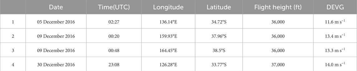
Table 1. The occurrence time (universal time), longitude and latitude, altitude, and turbulence intensity (i.e., DEVG) of these four cases.

Figure 1

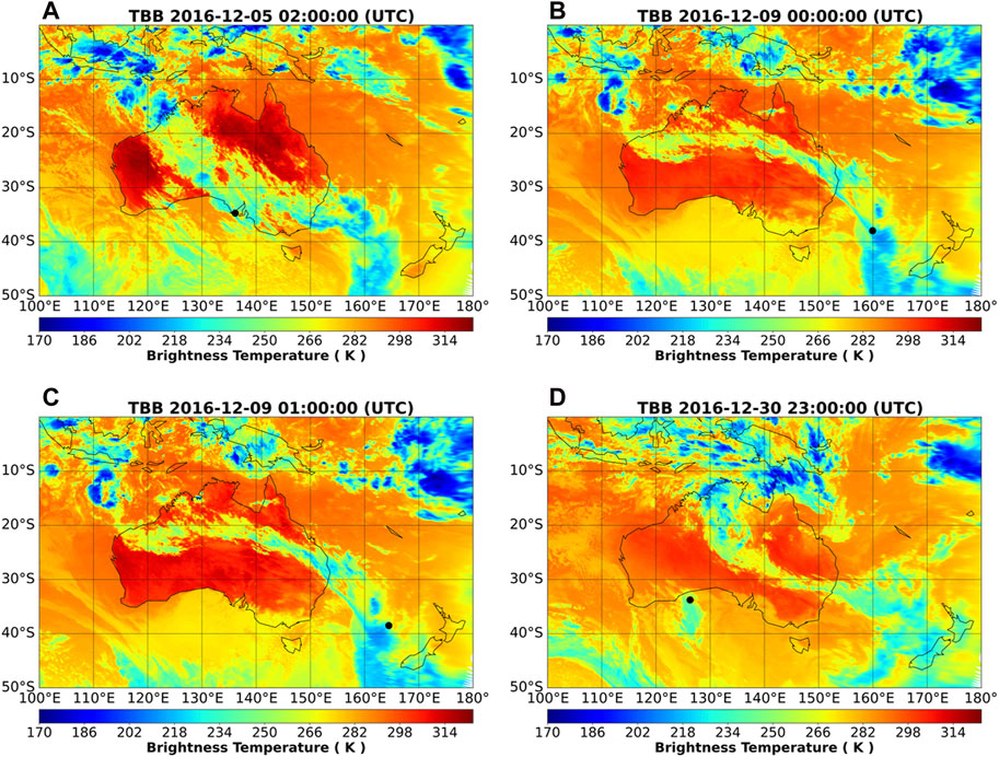
Figure 1. Black–body temperature (TBB) cloud map (unit: K) at the time of the four cases [(A): 0200 UTC 5 December 2016; (B): 0000 UTC 9 December 2016; (C): 0100 UTC 9 December 2016; (D): 2300 UTC 30 December 2016], where the black dots indicate the locations of the aircraft turbulence.

3.2 Analysis of circulation and physical characteristics of convective turbulence

For the four typical cases selected, analysis of the thermal and dynamic variables was performed to determine the characteristics of the convective turbulence and the key factors impacting aircraft turbulence near convective clouds.

3.2.1 Circulation characteristics of convective turbulence

In this section, the large–scale circulation characteristics of connective turbulence are analyzed, including the pressure field (geopotential height field), temperature field, and vector wind field in the low, middle, and upper troposphere. Exploring the key circulation systems and circulation factors at each level of the troposphere provides a large–scale circulation background for the subsequent analysis of the convective turbulence variables (Wang et al., 2018).

Figure 2 shows the distributions of the surface pressure field, temperature field, and vector wind field for the four cases of connective aircraft turbulence. It can be seen that during the turbulence event, there was always a warm high–pressure center south of Australia or in the southwest ocean, which has been discussed in other articles (Miyasaka and Nakamura, 2010). In particular, the high–pressure systems related to Cases 2 and 3 were very strong (Figures 2B, C). Moreover, the ocean southeast of Australia and west of New Zealand was mainly controlled by cold low–pressure systems on the ground, and aircraft turbulence often occurred between the high–and low–pressure systems. Additionally, it can be seen from the characteristics of the isotherms that aircraft turbulence occurred over areas with relatively large isotherm gradients, suggesting that the turbulence points were likely located near the front line.

Figure 2

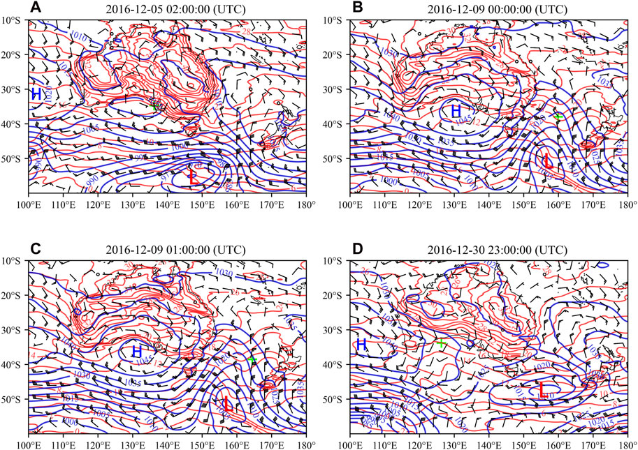
Figure 2. Distribution of sea level pressure (blue contours; unit: hPa), surface air temperature (red contours; unit: °C), and surface wind fields (barbs; unit: m·s⁻¹) at the time of the four cases [(A): 0200 UTC 5 December 2016; (B): 0000 UTC 9 December 2016; (C): 0100 UTC 9 December 2016; (D): 2300 UTC 30 December 2016]; The green plus sign indicates the location of the aircraft turbulence, and the letters “H” and “L” indicate the high– and low–pressure centers, respectively.

In the middle troposphere (500 hPa), the mid–to low–latitude areas in the Southern Hemisphere usually exhibit a weather pattern of two ridges and one trough during aircraft turbulence, with the high–pressure ridge on the west side is located over the area near 110∼120°E. During Cases 2 and 3, the high–pressure ridge on the east side was located between 150 and 160°E, and the intensity of the ridge was relatively strong. During Cases 1 and 4, the high–pressure ridge was located farther to the east, within 170∼180°E near New Zealand Island, and its intensity was relatively weak. Additionally, the subtropical high during Case 1 (588 geopotential line) was stronger and wider than those during the other three cases, and it controlled the weather over the northern part of Australia. During Cases 2, 3, and 4, the low–pressure troughs were all located near 140°E, whereas during Case 1, it was located near 160°E. A cut–off low pressure system can also be found on the east side of the trough during case 4, which were usually closed circulations in the middle and upper troposphere (Pinheiro et al., 2017). Furthermore, it can be seen from Figure 3 that convective turbulence mostly occurred in the northwest stream in front of the ridge behind the trough. The contours and isotherms in this area were relatively dense and the wind speed was high.

Figure 3

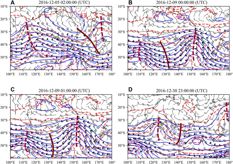
Figure 3. Distributions of 500 hPa geopotential height field (blue contours; unit: dagpm), air temperature field (red contours; unit: °C), and wind fields (barbs; unit: m·s⁻¹) at the time of the four cases [(A): 0200 UTC 5 December 2016; (B): 0000 UTC 9 December 2016; (C): 0100 UTC 9 December 2016; (D): 2300 UTC 30 December 2016]; The green plus sign indicates the location of the aircraft turbulence.

According to the altitudes of the turbulence points in Table 1, all four cases of aircraft turbulence occurred in the upper troposphere, that is, at ∼250 hPa. Figure 4 shows the geopotential height field, zonal wind field, and vector wind field in the upper troposphere (250 hPa) during the four cases. There was a significant high–pressure system in the upper troposphere. Compared with the high–pressure system in the lower troposphere, the location of the upper troposphere high–pressure system was slightly farther east and close to the locations of the high–pressure ridges on the east and west sides in the middle troposphere, indicating that the high–pressure system was a deep warm high–pressure system. All four cases of connective aircraft turbulence occurred in front of a deep warm high–pressure ridge where the contours (isotherms) were dense (i.e., large gradients) and there were strong northeasterly winds.

Figure 4

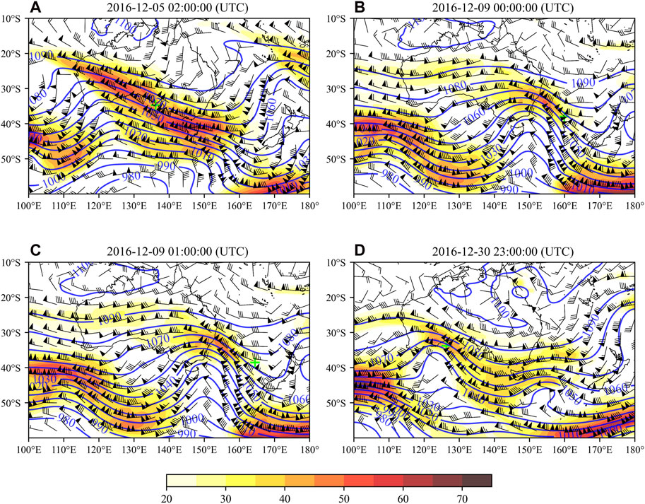
Figure 4. Distributions of 250 hPa geopotential height field (blue contours; unit: dagpm), zonal wind field (shadings; unit: m·s⁻¹), and wind fields (barbs; unit: m·s⁻¹) at the time of the four cases [(A): 0200 UTC 5 December 2016; (B): 0000 UTC 9 December 2016; (C): 0100 UTC 9 December 2016; (D): 2300 UTC 30 December 2016]; The green plus sign is the location of the aircraft turbulence.

In addition, the four cases all occurred near the subtropical westerly jet stream in the Southern Hemisphere, with wind speeds of ≥20 m·s^–1. In particular, the jet wind speed during Case 1 reached 60–70 m·s^–1. As can be seen from Figure 4, the turbulence point was located slightly to the left of the axis of the westerly jet stream where there was strong cyclonic wind shear and significant horizontal or vertical wind shear, which easily caused the occurrence of aircraft turbulence (Sharman et al., 2012).

3.2.2 Dynamic characteristics of convective turbulence

Aircraft turbulence is caused by atmospheric turbulence (Kim et al., 2018; Tenenbaum et al., 2022). The generation of atmospheric turbulence is governed by large–scale atmospheric motions. Atmospheric conditions that can easily trigger the occurrence and development of atmospheric turbulence are key factors that need to be considered when predicting aircraft turbulence.

The vorticity field, divergence field, and vertical speed field are fundamental dynamic fields that define atmospheric motion, and they describe the rotation speed and direction of the airflow, the change in volume, and the speed and direction of the vertical motion, respectively. In this section, the dynamic characteristics of convective turbulence are studied by analyzing the vorticity field, divergence field, vertical speed, horizontal wind shear, and vertical wind shear during the four cases of turbulence. As can be seen from Figure 5, the turbulence points of all four cases were not located in the extreme (positive or negative) divergence area but at the junction of the positive and negative divergence fields (i.e., near the zero–divergence line). That is, the turbulence occurred when the aircraft was passing through the transition area between the positive and negative divergence values, and the contours of the divergence field in this area were dense. According to the 250 hPa vorticity field, the aircraft avoided the high vorticity area in all four cases, yet the turbulence points were relatively close to the extreme (positive or negative) vorticity area where there was obvious vertical wind shear, which provided favorable conditions for the occurrence of aircraft turbulence. Therefore, the above results indicate that in the transition area between positive and negative divergence and vorticity areas, atmospheric turbulence is likely to develop due to the reversal of the motion and direction of the airflow. In particular, in the area with extreme (positive or negative) vorticity and nearly zero divergence, severe aircraft turbulence is likely to occur.

Figure 5

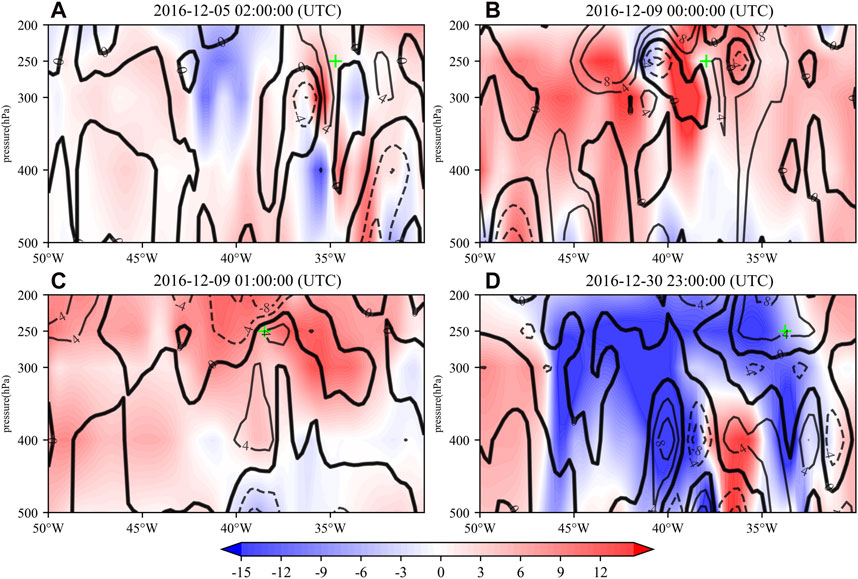
Figure 5. Longitude–pressure cross–section of divergence (contours; unit: 10⁻⁵ s⁻¹, bold line is the zero line) and vorticity (shadings; unit: 10⁻⁵ s^–1) along the latitudes of the turbulence locations in Table 1 at the time of the four cases [(A): 0200 UTC 5 December 2016; (B): 0000 UTC 9 December 2016; (C): 0100 UTC 9 December 2016; (D): 2300 UTC 30 December 2016]; The green plus sign indicates the location of the aircraft turbulence.

In addition, vertical airflow is a key factor that triggers atmospheric turbulence or aircraft turbulence (Sharman et al., 2012). Studies have shown that flying into vertical airflow and turbulence zones at a certain speed is one of the causes of aircraft turbulence. When an aircraft flies in an area of atmospheric turbulence, the speed and direction of the vertical wind changes significantly, resulting in drastic changes in the lift and causing aircraft turbulence. Next, we continue to explore the relationship between aircraft turbulence and the vertical airflow near convective clouds. Figure 6 shows a longitude–altitude profile of the vertical speed and specific humidity at 250 hPa along the latitude at which the turbulence point is located.

Figure 6

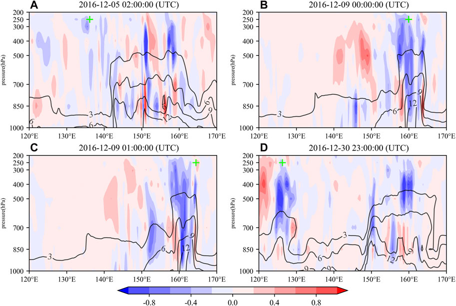
Figure 6. Longitude–pressure cross–section of 250 hPa vertical velocity (shadings; unit: Pa·s⁻¹) and specific humidity (contours; unit: g·kg^–1) along the latitudes of the turbulence locations in Table 1 at the time of the four cases [(A): 0200 UTC 5 December 2016; (B): 0000 UTC 9 December 2016; (C): 0100 UTC 9 December 2016; (D): 2300 UTC 30 December 2016]; The green plus sign indicates the location of the aircraft turbulence.

As shown in Figure 6, it can be seen that the turbulence points in all four cases were located near the area with strong ascending motions, and there was a thick moist layer in the middle and lower troposphere. This further validates that the cases in this study were all near-convective clouds turbulence events. In Cases 2, 3, and 4, the turbulence occurred next to the region with a prominently negative vertical speed, in the transition area between the positive and negative vertical speeds, indicating that the turbulence point was in the area with a strong vertical speed gradient, which is consistent with the above results based on the vorticity and divergence fields (Figure 6). Therefore, the positions of the four cases of aircraft turbulence were not only located to the left of the axis of the subtropical high–altitude jet stream but also in an area with a strong vertical speed gradient, that is, strong vertical wind shear and horizontal wind shear occurred in this area. As a result of the significant changes in the wind speed or direction, it was easy for aircraft turbulence to occur. In Case 1 (Figure 6A), the turbulence point was located on the west side of the ascending stream of the convective clouds and the deep moist layer. Despite of the large distance, the convective motion and the moist layer had a relatively wide influence, such that in Case 1, the aircraft was still in the transition area between the positive and negative vertical speeds, and there was also a certain vertical speed gradient.

3.2.3 Thermal characteristics of convective turbulence

By analyzing the temperature advection field around the turbulence point, the relationship between the temperature gradient, wind direction and speed, and aircraft turbulence was explored. Temperature advection is the phenomenon of the horizontal transport of temperature by the wind. It occurs when a warm or cold air mass moves into an area with a different temperature. The equation for calculating temperature advection is as follows:

$-\mathit{V}\bullet {\nabla }_{\mathit{h}}\mathit{T}=-\left(\mathit{u}\frac{\partial \mathit{T}}{\partial \mathit{x}}+\mathit{v}\frac{\partial \mathit{T}}{\partial \mathit{y}}\right)(5)$

where $-\mathit{V}\bullet {\nabla }_{\mathit{h}}\mathit{T}$ is the horizontal temperature advection, u and v are the zonal wind and meridional wind, respectively; T is the temperature, $\frac{\partial T}{\partial x}$ is the gradient of temperature in the latitudinal (east-west) direction, and $\frac{\partial T}{\partial y}$ is the gradient of temperature in the longitudinal (north-south) direction (Clark and Feldstein, 2020). The flow of air from a low–temperature area to a high–temperature area is referred to as cold advection, $-V·\nabla T<0$, and the air mass moves downward. The flow of air from a high–temperature area to a low–temperature area, which causes the temperature in the cold area to rise, which is called warm advection, $-V·\nabla T>0$, and the air mass moves upward. The occurrence of aircraft turbulence is caused by the vertical motion stimulated by the temperature advection at the edge of dense isotherms near the high–altitude jet streams. The frequency of aircraft turbulence is higher at the edge of dense isotherms near high–altitude jet streams than in other parts of the jet stream.

Figure 7 shows the distribution of the temperature advection at 250 hPa during the four near-convective clouds turbulence cases. It can be seen that the turbulence points during Cases 1, 2, and 3 were not located in the extreme area of temperature advection, but at the intersection or the boundary between the warm and cold advections, i.e., near the zero–temperature advection line. In the area, there was a large gradient between the warm and cold advections, which likely stimulated alternating upward and downward streams, and there were transition areas between the updraft and downdraft on both sides of the turbulence point. According to the route of the aircraft, it would pass the zero–temperature advection line, which is consistent with the above results based on the vertical speeds (Zhu, 1997). Moreover, during Cases 1, 2, and 3, positive and negative temperature advection occurred alternately near the turbulence points. Hence, the aircraft passed the zero–temperature advection line multiple times during its flight. Due to the different thermal properties of the air masses on both sides of the zero–temperature advection line, there was frequent vertical airflow in this area, making it easy for aircraft turbulence to occur. This is consistent with the conclusion based on the vertical speed (Figure 2). In conclusion, the turbulence cases 1, 2, and 3 corresponded well with the location of the zero–temperature advection line, and the temperature advection alternated between positive and negative values. The turbulence point during Case 4 was located in the positive temperature advection area, yet it was found that there were significant negative temperature advection areas both upstream and downstream of this area, indicating that positive and negative temperature advection also alternated near the turbulence point, resulting in significant vertical wind shear or vertical gusts and causing aircraft turbulence. Figure 8 illustrates the vertical wind shear and 250 hPa horizontal wind shear distribution during the four near-convective cloud turbulence events, calculated using Eqs 2, 4, respectively. It is evident that there was significant vertical wind shear during typical cases 1, 2, and 4, and noticeable horizontal wind shear during typical cases 2, 3, and 4, creating favorable conditions for the occurrence of aircraft turbulence. The conclusion remains consistent when examining the results of vertical and horizontal wind shear calculated using Formulas 2 and 4 (Figure 9).

Figure 7

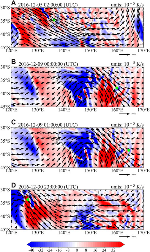
Figure 7. The 250 hPa temperature advection calculated from the Eq. 5 (shadings; unit: 10⁻⁵ K·s⁻¹) and wind field (vector; unit: m·s⁻¹) at the time of the four cases [(A): 0200 UTC 5 December 2016; (B): 0000 UTC 9 December 2016; (C): 0100 UTC 9 December 2016; (D): 2300 UTC 30 December 2016]; The green dots indicate the locations of the aircraft turbulence.

Figure 8

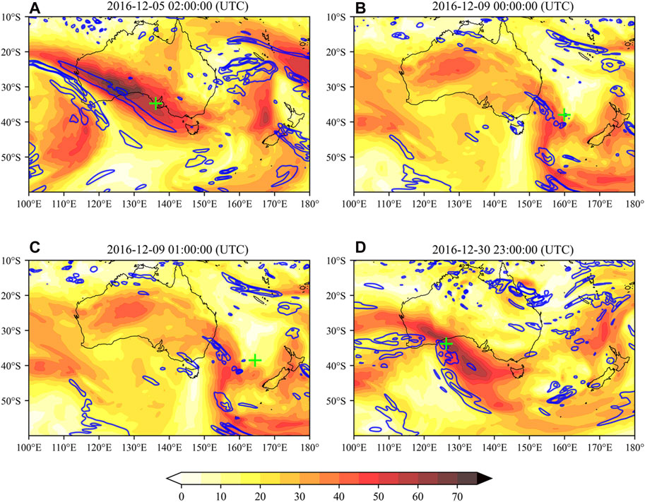
Figure 8. Distribution of vertical wind shear calculated from the Eq. 1 (shadings; units: m·s⁻¹) and 250 hPa horizontal wind shear calculated from the Eq. 4 (contours are 2, 4, 6 s⁻¹) during the four turbulence cases [(A): 0200 UTC 5 December 2016; (B): 0000 UTC 9 December 2016; (C): 0100 UTC 9 December 2016; (D): 2300 UTC 30 December 2016]; The green plus sign indicates the location of aircraft turbulence.

Figure 9

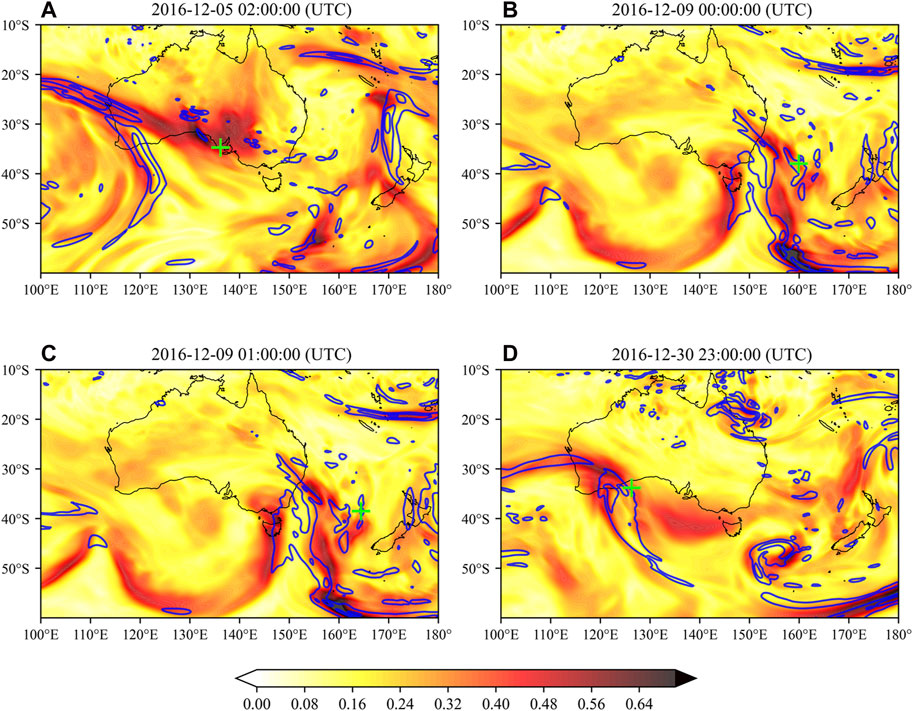
Figure 9. Distribution of vertical wind shear calculated from the Eq. 2 (shadings; units: s⁻¹) and 250 hPa horizontal wind shear calculated from the Eq. 4 (contours are 8, 14, 20 s⁻¹) during the four turbulence cases [(A): 0200 UTC 5 December 2016; (B): 0000 UTC 9 December 2016; (C): 0100 UTC 9 December 2016; (D): 2300 UTC 30 December 2016]; The green plus sign indicates the location of aircraft turbulence.

Next, the European Centre for Medium–Range Weather Forecasts (ECMWF) ERA5 climate reanalysis data were used to calculate the vertical profiles of the pseudo–equivalent potential temperature (${\theta }_{se}$) along the latitude (longitude) of the turbulence points for the four cases so as to further analyze the atmospheric stability characteristics around the turbulence locations. As shown in Figures 10, 11, the pseudo–equivalent potential temperature near the convective clouds shifted towards the cold area with increasing altitude, and the turbulence point was located in the area with large pseudo–equivalent potential temperature gradients. The results suggest that the horizontal temperature gradient in the frontal zone was much larger than that of the air masses on both sides of the frontal zone, and there were dense isotherms near the frontal zone (Yuan and Talley, 1996; June 2007). The frontal zone is the area containing dense isotherms on the isobaric surface map. Therefore, the four cases of aircraft turbulence may have occurred near the high–altitude frontal zone, which is consistent with the conclusion illustrated in Figure 2. Since the warm air obliquely covered the cold air, the vertical temperature gradient was much smaller in the frontal zone than in the air masses on both sides, and sometimes, there was even a temperature inversion phenomenon, that is, the temperature increased with altitude. As shown in Figure 10, in all four cases, inversion of the pseudo–equivalent potential temperature (i.e., the convective unstable stratification $\partial {\theta }_{se}⁄\partial p>0$, occurred in the middle and lower troposphere near the turbulence locations (warm air side) and distributed in the range of 10∼30°S. The unstable stratification of cold air at the top and warm air at the bottom was conducive to triggering convection from the ground, forming strong convective clouds and causing severe turbulence (Murakami et al., 2003; Liu et al., 2020). In addition, in Cases 1 and 3, the southerlies in the lower troposphere and the northerlies in the upper troposphere induced strong vertical wind shear, resulting in a certain degree of baroclinicity and promoting the development of convective turbulence. This is consistent with the findings illustrated Figure 8. In Cases 2, 3, and 4, significant vertical airflow occurred on the cold side of the turbulence points, and the wind speeds on both sides of the turbulence point were significantly different at the same altitude, indicating the occurrence of strong horizontal wind shear in this area, which was conducive to the occurrence of aircraft turbulence (Figures 10B–D, 11B–D).

Figure 10

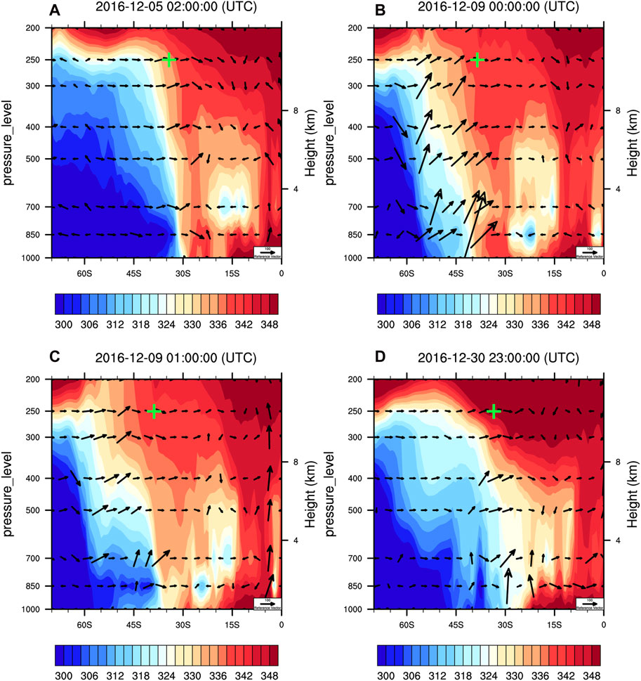
Figure 10. Latitude–pressure cross section of the pseudo–equivalent potential temperature (shadings; unit: K) and the wind field (the arrows represent the composite wind vectors of u and ω×250) along the longitudes of the turbulence locations at the time of the four cases [(A): 0200 UTC 5 December 2016; (B): 0000 UTC 9 December 2016; (C): 0100 UTC 9 December 2016; (D): 2300 UTC 30 December 2016]; The green plus sign indicates the location of aircraft turbulence (Flight altitude was selected at 250 hPa).

Figure 11

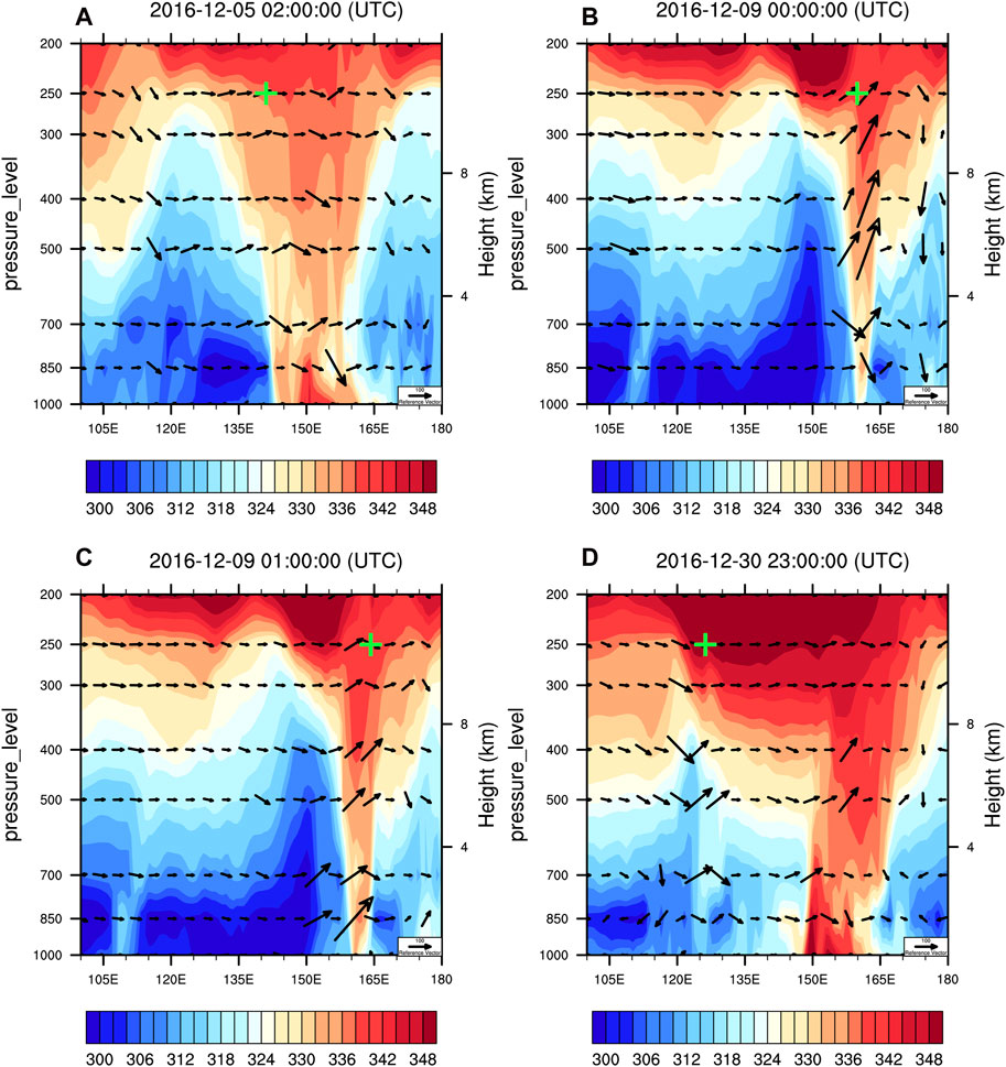
Figure 11. Longitude–pressure cross section of the pseudo–equivalent potential temperature (shadings; unit: K) and the wind field (the arrows represent the composite wind vectors of u and ω×250) along the latitudes of the turbulence locations at the time of the four cases [(A): 0200 UTC 5 December 2016; (B): 0000 UTC 9 December 2016; (C): 0100 UTC 9 December 2016; (D): 2300 UTC 30 December 2016]; The green plus sign indicates the location of aircraft turbulence (Flight altitude was selected at 250 hPa).

4 Conclusion

Based on four typical cases of near-convective clouds turbulence over Australia, this study analyzed the large–scale circulation background of these convective turbulence events. By analyzing such variables as the vertical speed, divergence and vorticity, vertical and horizontal wind shear, temperature advection, and pseudo–equivalent potential temperature, the thermal and dynamic characteristics of the aircraft turbulence near convective clouds were quantified. The conclusions of this study are as follows.

(1) During near-connective clouds turbulence, the middle to low–latitude areas in the Southern Hemisphere usually exhibit a weather pattern characterized by two ridges and one trough. In the four cases analyzed in this study, convective turbulence mostly occurred in the northwest stream in front of the ridge behind the trough. This area was in front of a deep warm high–pressure ridge where the contours (isotherms) were dense (i.e., large gradients) and there were strong northeasterly winds. Additionally, the turbulence points of all four cases were located slightly to the left of the axis of the westerly jet stream where there was strong cyclonic wind shear and significant horizontal or vertical wind shears, which easily caused the occurrence of aircraft turbulence.

(2) The turbulence points of all four cases were located at the junction between the positive and negative divergence or vorticity fields (i.e., near the zero–divergence/vorticity line). That is, the turbulence occurred when the aircraft was passing through the transition area between the positive and negative divergence and vorticity areas. In the transition area, atmospheric turbulence was likely to develop due to the reversal of the motion and direction of the airflow. In particular, in the area with extreme (positive or negative) vorticity and nearly zero divergence, severe aircraft turbulence is likely to occur. In addition, convective turbulence usually occurs in an area with a large vertical speed gradient where there are strong vertical and horizontal wind shears that can easily trigger aircraft turbulence.

(3) The turbulence points were located at the intersection or boundary between warm and cold advections, i.e., near the zero–temperature advection line. In this area, there was a large gradient between the warm and cold advection, which likely stimulated alternating upward and downward airstreams. Moreover, turbulence occurred near the high–altitude frontal zones, and inversion of the pseudo–equivalent potential temperature occurred in the middle and lower troposphere near the turbulence point (on the warm air side). The unstable stratification pattern of cold air at the top and warm air at the bottom occurred in the upper part of the frontal zone, which was conducive to triggering convection from the surface, forming strong convective clouds, and causing aircraft turbulence.

5 Discussion

Four typical severe near-convective clouds turbulence events over the Australia have been examined in present study. Expanding the analysis to more events and other regions in the following study can significantly strengthen the above conclusions. A deeper exploration of the possible physical mechanisms behind the observed relationships in present study will be conducted in the future work. For example, the formation mechanism of the significant vertical and horizontal wind shear near these turbulence points will be revealed by analyzing the gravity wave breaking or other external forcing factors.

Data availability statement

The datasets presented in this study can be found in online repositories. The names of the repository/repositories and accession number(s) can be found in the article/Supplementary Material.

Author contributions

YW: Software, Writing–original draft. CW: Funding acquisition, Methodology, Writing–review and editing. RW: Formal Analysis, Writing–review and editing. RN: Data curation, Writing–review and editing.

Funding

The authors declare that financial support was received for the research, authorship, and/or publication of this article. This research was jointly Supported by Sichuan Science and Technology Program, grant number 2022NSFSC1149, and the Fundamental Research Funds for the Central Universities, grant number J2020–083 and TS–06.

Acknowledgments

Special thanks to the reviewers for their valuable comments.

Conflict of interest

The authors declare that the research was conducted in the absence of any commercial or financial relationships that could be construed as a potential conflict of interest.

Publisher’s note

All claims expressed in this article are solely those of the authors and do not necessarily represent those of their affiliated organizations, or those of the publisher, the editors and the reviewers. Any product that may be evaluated in this article, or claim that may be made by its manufacturer, is not guaranteed or endorsed by the publisher.

References

Bramberger, M., Drnbrack, A., Wilms, H., Ewald, F., and Sharman, R. (2020). MountainWave turbulence encounter of research aircraft HALO above Iceland. J. Appl. Meteorology Climatol. 59 (3), 567–588. doi:10.1175/JAMC–D–19–0079.1

CrossRef Full Text | Google Scholar

Cai, W. J., Gao, L. B., Luo, Y. Y., Li, X. C., Zheng, X. T., Zhang, X. B., et al. (2023b). Sourn Ocean warming and its climatic impacts. Sci. Bull. 68 (9), 946–960. doi:10.1016/j.scib.2023.03.049

CrossRef Full Text | Google Scholar

Cai, X. W., Wan, Z. W., Wu, W. H., Yang, B., and Yi, Z. H. (2023a). An ensemble prediction method of aviation turbulence based on energy dissipation rate. Chin. J. Atmos. Sci. (in Chinese) 47 (4), 1085–1098. doi:10.3878/j.issn.1006–9895.2112.21147

CrossRef Full Text | Google Scholar

Clark, J. P., and Feldstein, S. B. (2020). What drives north atlantic oscillation’s temperature anomaly pattern? Part I: growth and decay of surface air temperature anomalies. Journal of Atmospheric Science 77, 185–198. doi:10.1175/JAS–D–19–0027.1

CrossRef Full Text | Google Scholar

Colson, D., and Panofsky, H. A. (1965). An index of clear air turbulence. Quarterly Journal of Royal Meteorological Society 91, 507–513. doi:10.1002/qj.49709139010

CrossRef Full Text | Google Scholar

Ellrod, G. P., and Knox, J. A. (2010). Improvements to an operational clear-air turbulence diagnostic index by addition of a divergence trend term. Wear and Forecasting 25 (2), 789–798. doi:10.1175/2009WAF2222290.1

CrossRef Full Text | Google Scholar

Gill, P. G. (2014). Objective verification of world area forecast centre clear air turbulence forecasts. Meteorological Applications 21 (1), 3–11. doi:10.1002/met.1288

CrossRef Full Text | Google Scholar

Huang, R. S., Sun, H. B., Wu, C., Wang, C., and Lu, B. B. (2019). Estimating eddy dissipation rate with QAR flight big data. Applied Sciences 9 (23), 5192. doi:10.3390/app9235192

CrossRef Full Text | Google Scholar

Huang, Y. F., Sun, Z. B., Xiao, H. Q., and Xu, W. (2010). The large–scale cloud system and its distribution that makes airplane turbulence in plateau of China. Plateau and Mountain Meteorology Research 30 (2), 42–45. (in Chinese). doi:10.3969/j.issn.1674-2184–2010.02.009

CrossRef Full Text | Google Scholar

Jun, M. (2007). Large–scale features associated with frontal zone over east asia from late summer to autumn. Journal of Meteorological Society of Japan 66 (4), 565–579. doi:10.2151/jmsj1965.66.4_565

CrossRef Full Text | Google Scholar

Kaluza, T., Kunkel, D., and Hoor, P. (2022). Analysis of turbulence reports and ERA5 turbulence diagnostics in a tropopause-based vertical framework. Geophysical Research Letters 49, e2022GL100036. doi:10.1029/2022GL100036

CrossRef Full Text | Google Scholar

Kim, J. H., Chun, H. Y., Sharman, R. D., and Keller, T. L. (2011). Evaluations of upper-level turbulence diagnostics performance using graphical turbulence guidance (GTG) system and pilot reports (PIREPs) over east asia. Journal of Applied Meteorology and Climatology 50 (9), 1936–1951. doi:10.1175/JAMC–D–10–05017.1

CrossRef Full Text | Google Scholar

Kim, J. H., Sharman, R., Strahan, M., Scheck, J. W., Bartholomew, C., Cheung, J. C. H., et al. (2018). Improvements in nonconvective aviation turbulence prediction for world area forecast system. Bulletin of American Meteorological Society 99, 2295–2311. doi:10.1175/BAMS–D–17–0117.1

CrossRef Full Text | Google Scholar

Kim, S. H., and Chun, H. Y. (2016). Aviation turbulence encounters detected from aircraft observations: spatiotemporal characteristics and application to Korean Aviation Turbulence Guidance. Meteorological Applications 23 (4), 594–604. doi:10.1002/met.1581

CrossRef Full Text | Google Scholar

Kim, S. H., Chun, H. Y., Kim, J. H., Sharman, R., and Strahan, M. (2020). Retrieval of eddy dissipation rate from derived equivalent vertical gust included in Aircraft Meteorological Data Relay (AMDAR). Atmospheric Measurement Techniques 13 (3), 1373–1385. doi:10.5194/amt–13–1373–2020

CrossRef Full Text | Google Scholar

Lane, T. P., Sharman, R. D., Trier, R. G., and Williams, J. (2012). Recent advances in understanding of near–cloud turbulence. Bulletin of American Meteorological Society 93, 499–515. doi:10.1175/BAMS–D–11–00062.1

CrossRef Full Text | Google Scholar

Lee, J. H., Kim, J. H., Sharman, R. D., and Son, S. (2023). Climatology of clear-air turbulence in upper troposphere and lower stratosphere in Norrn Hemisphere using ERA5 reanalysis data. Journal of Geophysical Research Atmospheres 128 (1), e2022JD037679. doi:10.1029/2022JD037679

CrossRef Full Text | Google Scholar

Li, Z. L., and Huang, Y. F. (2008). Gravity wave and inertial instability—possible mechanism of atmospheric turbulence and airplane bumps. Plateau Meteorology 27 (4), 859–865. (in Chinese). doi:10.3724/SP.J.1047.2008.00014

CrossRef Full Text | Google Scholar

Liao, J., and Xiong, A. Y. (2010). Introduction and quality analysis of Chinese aircraft meteorological data. Chinese Journal of Applied Meteorological Science 21 (2), 206–213. (in Chinese). doi:10.3724/SP.J.1084.2010.00199

CrossRef Full Text | Google Scholar

Liu, Z. Y., Yu, H. P., Sheng, X., Zhu, C. Q., Zhao, Q. Y., Ma, Y. X., et al. (2020). Mechanism analysis of a rare “thunder snow” process in semi–arid area. Meteorological Monthly 46 (12), 1596–1607. (in Chinese). doi:10.7519/j.issn.1000–0526.2020.12.007

CrossRef Full Text | Google Scholar

Mazon, J. B., Rojas, J. I. G., Lozano, M., Pino, D., Prats, X., and Miglietta, M. M. (2018). Influence of meteorological phenomena on worldwide aircraft accidents in period 1967–2010. Meteorlogical Applications 24 (5), 236–245. doi:10.1002/met.1686

CrossRef Full Text | Google Scholar

Meneguz, E., Wells, H., and Turp, D. (2016). An automated system to quantify aircraft encounters with convectively induced turbulence over europe and norast atlantic. Journal of Applied Meteorology and Climatology 55, 1077–1089. doi:10.1175/JAMC–D–15–0194.1

CrossRef Full Text | Google Scholar

Misaka, T., Obayashi, S., and Endo, E. (2008). Measurement–Integrated simulation of clear air turbulence using a four–dimensional variational method. Journal of Aircraft 45 (4), 1217–1229. doi:10.2514/1.34111

CrossRef Full Text | Google Scholar

Miyasaka, T., and Nakamura, H. (2010). Structure and mechanisms of sourn hemisphere summertime subtropical anticyclones. Journal of Climate 23, 2115–2130. doi:10.1175/2009JCLI3008.1

CrossRef Full Text | Google Scholar

Murakami, M., Yamada, Y., Matsuo, T., Iwanami, K., Marwits, J., and Gordon, G. (2003). Precipitation process in convective cells embedded in deep snow bands over sea of Japan. Journal of Meteorological Society of Japan 81 (3), 515–531. doi:10.2151/jmsj.81.515

CrossRef Full Text | Google Scholar

Palmer, C. K., and Barnes, G. M. (2002). Effect of vertical wind shear as diagnosed by NCEP/NCAR Reanalysis data on Norast Pacific hurricane intensity. San Diego, CA: Preprints, AMS, 25th Hurricane and Tropical Meteorology, 122–123.

Google Scholar

Pinheiro, H. R., Hodges, K. I., Gan, M. A., and Ferreira, N. J. (2017). A new perspective of climatological features of upper–level cut–off lows in Sourn Hemisphere. Climate Dynamics 48, 541–559. doi:10.1007/s00382–016–3093–8

CrossRef Full Text | Google Scholar

Prosser, M. C., Williams, P. D., Marlton, G. J., and Harrison, R. G. (2023). Evidence for large increases in clear–air turbulence over past four decades. Geophysical Research Letters 50 (11), e2023GL103814. doi:10.1029/2023GL103814

CrossRef Full Text | Google Scholar

Rodriguez, I. P., Mininni, P. D., Godoy, A., Rivaben, N., and Dörnbrack, A. (2023). Not all clear air turbulence is Kolmogorov— fine-scale nature of atmospheric turbulence. Journal of Geophysical Research Atmospheres 128 (2), e2022JD037491. doi:10.1029/2022JD037491

CrossRef Full Text | Google Scholar

Schultz, D. M., Kanak, K. M., Straka, J. M., Trapp, R. J., Gordon, B. A., Zrnić, D. S., et al. (2006). Mysteries of mammatus clouds: observations and formation mechanisms. J. Atmos. Sci. 63, 2409–2435. doi:10.1175/JAS3758.1

CrossRef Full Text | Google Scholar

Sekizawa, S., Nakamura, H., and Kosaka, Y. (2018). Interannual variability of Australian summer monsoon system internally sustained through wind-evaporation feedback. Geophysical Research Letters 45, 7748–7755. doi:10.1029/2018GL078536

CrossRef Full Text | Google Scholar

Sharman, R., and Bernstein, B. C. (2022). “Climatology study of aircraft turbulence versus cloud cover [poster],” in 10th conference on aviation, range, and aerospace meteorology (Portland, OR, US: American Meteorological Society).

Google Scholar

Sharman, R., Tebaldi, C., Wiener, G., and Wolff, J. (2006). An integrated approach to mid–and upper–level Turbulence forecasting. Wear Forecasting 21 (3), 268–287. doi:10.1175/WAF924.1

CrossRef Full Text | Google Scholar

Sharman, R. D., Trier, S. B., Lane, T. P., and Doyle, J. D. (2012). Sources and dynamics of turbulence in upper troposphere and lower stratosphere: a review. Geophysical Research Letters 39 (12), L12803. doi:10.1029/2012GL051996

CrossRef Full Text | Google Scholar

Sherman, D. J. (1985). Australian implementation of AMDAR/ACARS and use of derived equivalent gust velocity as a turbulence indicator. Aeronautical Research Laboratories Structures Rep, 1–42.

Google Scholar

Tenenbaum, J., Williams, P. D., Turp, D., Buchnan, P., Coulson, R., Gill, P. G., et al. (2022). Aircraft observations and reanalysis depictions of trends in North Atlantic winter jet stream wind speeds and turbulence. Quarterly Journal of Royal Meteorological Society 148 (747), 2927–2941. doi:10.1002/qj.4342

CrossRef Full Text | Google Scholar

Trier, S. B., and Sharman, R. D. (2016). Mechanisms influencing cirrus banding and aviation turbulence near a convectively enhanced upper–level jet stream. Monthly Wear Review 144 (8), 3003–3027. doi:10.1175/MWR–D–16–0094.1

CrossRef Full Text | Google Scholar

Wang, L. J., Wang, C., and Guo, D. (2018). Evolution mechanism of synoptic–scale EAP teleconnection pattern and its relationship to summer precipitation in China. Atmospheric Research 214, 150–162. doi:10.1016/j.atmosres.2018.07.023

CrossRef Full Text | Google Scholar

Wang, Y. Z. (2006). Effect of air turbulence on airplane turbulence. Journal of Southwest Jiaotong University 19 (3), 279–283. (in Chinese).

Google Scholar

Wang, Y. Z., and Zhu, W. J. (2001). A formation mechanism of air turbulence jet stream ravitational wave of boundary layer. Transactions of Atmospheric Sciences 24 (3), 429–432. (in Chinese).

Google Scholar

Wen, Y., Zhang, Q. L., and Xu, J. Y. (2019). Propagation characteristics of mesospheric concentric gravity waves excited by a thunderstorm. Chinese Journal of Geophysics 62 (4), 1218–1229. doi:10.6038/cjg2019M0186

CrossRef Full Text | Google Scholar

Williams, P. D., and Joshi, M. M. (2013). Intensification of winter transatlantic aviation turbulence in response to climate change. Nature Climate Change 3 (7), 644–648. doi:10.1038/NCLIMATE1866

CrossRef Full Text | Google Scholar

Yoshimura, R., Suzuki, K., Ito, J., Kikuchi, R., Yakeno, A., and Obayashi, S. (2022). Large–Eddy and flight simulations of a clear–air turbulence event over Tokyo on 16 december 2014. Journal of Applied Meteorology and Climatology 61 (5), 503–519. doi:10.1175/JAMC–D–21–0071.1

CrossRef Full Text | Google Scholar

Yu, J. H., Tan, Z. M., and Wang, Y. Q. (2010). Effects of vertical wind shear on intensity and rainfall asymmetries of strong Tropical Storm Bilis (2006). Advances in Atmospheric Sciences 27 (3), 552–561. doi:10.1007/s00376-009-9030-6

CrossRef Full Text | Google Scholar

Yuan, X., and Talley, L. D. (1996). Subarctic frontal zone in North Pacific: characteristics of frontal structure from climatological data and synoptic surveys. Journal of Geophysical Research Oceans 101 (C7), 16491–16508. doi:10.1029/96jc01249

CrossRef Full Text | Google Scholar

Zhu, Z. Y. (1997). Analysis of a formation mechanism on airplane turbulence in upper jet stream. Journal of Chengdu Institute of Meteorology 12 (4), 21–26. (in Chinese).

Google Scholar