Full waveform inversion based on deep learning and the phase-preserving symplectic partitioned Runge-Kutta method

To obtain more accurate full waveform inversion results, we present a forward modeling method with minimal phase error, low numerical dispersion, and high computational efficiency. To solve the 2D acoustic wave equation, we utilize a finite-difference (FD) scheme with optimized coefficients for spatial discretization, combined with a phase-preserving symplectic partitioned Runge-Kutta method for temporal discretization. This results in the development of the optimized symplectic partitioned Runge-Kutta (OSPRK) forward modeling method. We further apply the OSPRK method in conjunction with a recurrent neural network (RNN) for full waveform inversion (FWI). Our study explores the impact of various loss functions, Nadam optimizer parameters, and the incorporation of physical information operators on inversion performance. Numerical experiments demonstrate that the OSPRK method significantly reduces numerical dispersion compared to traditional FD methods. The Log-Cosh loss function offers superior stability across different learning rates, while the Nesterov-accelerated Adaptive Moment Estimation (Nadam) optimizer with optimized parameters greatly enhances convergence speed and inversion accuracy. Furthermore, the inclusion of physical information operators markedly improves inversion outcomes.

1 Introduction

Full waveform inversion (FWI) is widely used in oil and gas exploration, geotectonic research, and infrastructure development. This technique relies on the analysis of seismic waveforms, which propagate through subsurface media and are recorded by receivers, to infer the material properties of the Earth’s interior (Tarantola, 1984; Virieux and Operto, 2009; Tong et al., 2014). In this process, the wave equation is typically employed to simulate the propagation of seismic waves through the medium, producing synthetic waveform data. An optimization algorithm is then applied to iteratively refine the subsurface parameters, improving the accuracy of the inversion with each iteration.

In FWI, solving the wave equation represents the primary computational burden. As a result, the development of numerical methods that can solve wave equations with both high accuracy and efficiency has been a key area of research. Numerical methods for wave equation solutions involve spatial discretization, time discretization, and boundary condition handling. Spatial discretization methods include the traditional finite difference (FD) method (Virieux, 1986; Moczo et al., 2002; Saenger et al., 2004), the finite element method (Eriksson and Johnson, 1991; Yang et al., 2008), the nearly analytic discrete (NAD) method (Yang et al., 2003), the optimized finite difference format (Zhang and Yao, 2013), the optimized expansion method (Wu and Alkhalifah, 2014), among others. The FD method tends to perform well when using a fine mesh but suffers from significant numerical dispersion when applied with a coarse mesh (Yang et al., 2006; Ma et al., 2020; Wu and Alkhalifah, 2018). The NAD method improves on this by utilizing both displacement and gradient information from grid points and their neighbors to approximate higher-order spatial derivatives, thereby reducing numerical dispersion. However, this method requires substantial computational resources, which limits its efficiency. Zhang and Yao (2013) introduced an optimized FD method that minimizes wave number errors using the maximum norm. The optimized coefficients for this method are obtained via the simulated annealing technique (Kirkpatrick et al., 1983), resulting in lower numerical dispersion and greater computational efficiency. For temporal discretization, methods include the symplectic partitioned Runge-Kutta (SPRK) method (Qin and Zhang, 1990), the phase-preserving SPRK (Ma and Yang, 2017), and the modified SPRK format (Liu et al., 2017). Each method has distinct advantages depending on the application. For instance, Liu et al. (2017) introduced a modified SPRK method that achieves higher-order accuracy with reduced computational cost. Ma and Yang, (2017) developed optimized coefficients for the phase-preserving SPRK format, which significantly reduces phase errors and improves overall accuracy.

In recent years, with the rapid advancement of deep learning technologies, researchers have begun integrating deep learning with forward modeling and inversion techniques in geophysics. Richardson (2018) was the first to combine forward modeling with the recurrent neural network (RNN) framework in deep learning. His numerical experiments showed that the Adam optimizer in deep learning outperformed the traditional L-BFGS-B optimizer for inversion tasks. Wu and McMechan (2019) applied convolutional neural networks (CNNs) to generate initial velocity models by utilizing a weighting parameter, resulting in inverted velocity models that were more accurate than those produced by conventional FWI methods. Raissi et al. (2019) introduced Physics-Informed Neural Networks (PINN) to tackle both forward and inverse problems involving nonlinear partial differential equations, a method later extended by Song and Alkhalifah (Song and Alkhalifah, 2021). Lu et al. (2021) further refined this approach by integrating high-precision operators into the RNN framework and enhancing the loss function of FWI through the incorporation of physical information operators, leading to improved inversion accuracy. Li et al. (2021) improved the resolution of the elastic full waveform inversion (EFWI) by using a deep neural network to learn the statistical relationship between selected features in the inversion model and the lithology interpreted from downhole logs. Li et al. (2023) designed a deep learning (DL) framework that combines full waveform inversion (FWI) on seismic data and downhole logging information to construct a subsurface model, which ultimately improves the resolution and accuracy of the velocity model.

The innovation of this study lies in the use of the OSPRK method as the forward modeling approach for FWI, along with the Log_Cosh function enhanced by physically informed operators as the loss function. In cases involving coarse grids, traditional FD methods tend to introduce significant numerical dispersion, resulting in greater numerical errors with each iteration of the inversion process. In contrast, the OSPRK method is characterized by its low numerical dispersion and minimal phase error, making it superior to the FD method. The Log_Cosh loss function combines the advantages of both the Mean Squared Error (MSE) and Mean Absolute Error (MAE) loss functions. By incorporating a physical information operator that adheres to the wave equation into this loss function, we impose a constraint based on physical principles, thereby improving the accuracy of the inversion results.

2 OSPRK method

2.1 OSPRK for solving the two-dimensional acoustic equation

A 2n-dimensional linear separable Hamiltonian system can be written in the following form (Feng and Qin, 2010):

$\left\{\begin{array}{l}\frac{\mathrm{\partial }u}{\mathrm{\partial }t}=f\left(v\right)\\ \frac{\mathrm{\partial }v}{\mathrm{\partial }t}=g\left(u\right)\end{array}\right.,(1)$

where $u$ and $v$ are the generalized coordinate and momentum, respectively, and $f$ and $g$ are linear functions of $v$ and $u$, respectively.

Solving Equation 1 in kth order SPRK format (Ma and Yang, 2017) can be expressed as:

$\left\{\begin{array}{l}{u}_0=u^n,v_0=v^n\\ u_i=u_{i-1}+c_i\Delta tf\left(v_{i-1}\right)\\ v_i=v_{i-1}+d_i\Delta tg\left(u_i\right),i=1,2,\cdots ,k\\ u^{n+1}=u_k,v^{n+1}=v_k\end{array}\right.,$

where $\Delta t$ is the time increment, and $c_i\left(i=1,2,\cdots ,k\right)$ and $d_i\left(j=1,2,\cdots ,k\right)$ are the system coefficients of the SPRK. $v^n$ and $u^n$ are numerical solutions for the nth time step of the system, and $v_i$ and $u_i$ are intermediate variables of the format.

In a two-dimensional isotropic medium with constant density, the acoustic wave equation can be expressed as:

$\frac{{\mathrm{\partial }}^{2}u}{\mathrm{\partial }{t}^2}=s^2\left(x,z\right)\left(\frac{{\mathrm{\partial }}^{2}u}{\mathrm{\partial }{x}^2}+\frac{{\mathrm{\partial }}^{2}u}{\mathrm{\partial }{z}^2}\right),(2)$

where $s$, $u$ and $t$ denotes the velocity of the acoustic wave propagating in the medium, displacement, and time, respectively. By introducing the variable $v=\frac{\mathrm{\partial }u}{\mathrm{\partial }t}$, we can transform Equation 2 into a linearly differentiable Hamiltonian system (Qin and Zhang, 1990). The transformed equation is written as:

$\left\{\begin{array}{l}\frac{du}{dt}=v\\ \frac{dv}{dt}=Lu\end{array}\right.,(3)$

where $v$ is the velocity, and $L=s^2\left(\frac{{\mathrm{\partial }}^2}{\mathrm{\partial }{x}^2}+\frac{{\mathrm{\partial }}^2}{\mathrm{\partial }{z}^2}\right)$ is the spatial operator of the wave equation. Then Equation 3 conforms to the form of Equation 1. The linear separable Hamiltonian system of wave equation can be written in the following form:

$\left\{\begin{array}{l}{u}_0=u^n,v_0=v^n\\ u_i=u_{i-1}+c_i\Delta t{v}_{i-1}\\ v_i=v_{i-1}+d_i\Delta tL{u}_i,i=1,2\cdots k\\ u^{n+1}=u_k,v^{n+1}=v_k\end{array}\right.,(4)$

We employ the fourth-order SPRK format for temporal discretization. Equation 4 is then expressed as:

$\left\{\begin{array}{l}{u}_1=u_n+c_1\Delta t{v}^n\\ v_1=v^n+d_1\Delta tL{u}_1\\ u_2=u_1+c_2\Delta t{v}_1\\ v_2=v_1+d_2\Delta tL{u}_2\\ u_3=u_2+c_3\Delta t{v}_2\\ v_3=v_2+d_3\Delta tL{u}_3\\ u^{n+1}=u_3+c_4\Delta t{v}_3\\ v^{n+1}=v_3+d_4\Delta tL{u}^{n+1}\end{array}\right.,(5)$

For the temporal discretization, Ma and Yang, (2017) derived a vector of coefficients corresponding to the fourth-order phase-preserving SPRK for the individual coefficients of $c_i\left(i=1,2,3,4\right)$ and $d_i\left(i=1,2,3,4\right)$:

$\left\{\begin{array}{l}{c}_1=0.263343\\ c_2=-0.048643\\ c_3=0.412664\\ c_4=0.372618\end{array}\right.,\left\{\begin{array}{l}{d}_1=-0.359822\\ d_2=0.751499\\ d_3=0.469686\\ d_4=0.138837\end{array}\right..$

For second-order derivatives in $L$, the optimized finite difference format for its sixth-order can be written as follows:

${\left.\frac{{\mathrm{\partial }}^{2}u}{\mathrm{\partial }{x}^2}\right|}_{x=x_0}={\displaystyle \sum _{j=-3}^3}{b}_{j}u\left(x_0+j\Delta x\right),$

where the coefficients of the sixth-order optimized finite difference operator (Zhang and Yao, 2013) are as follows:

$\left\{\begin{array}{l}{b}_0=-2.821545\\ b_1=1.576632\\ b_2=-0.183472\\ b_3=0.017613\\ b_j=b_{-j}\left(j=1,2,3\right)\end{array}\right.,$

To prevent unwanted reflections at the edges of the simulation domain, we incorporate the perfectly matched layer (PML) (Wang, 2003) into Equation 5. Consequently, the complete process for solving the wave equation involves temporal discretization, spatial discretization, and the implementation of the PML to absorb outgoing waves effectively.

2.2 OSPRK-RNN method for seismic inversion

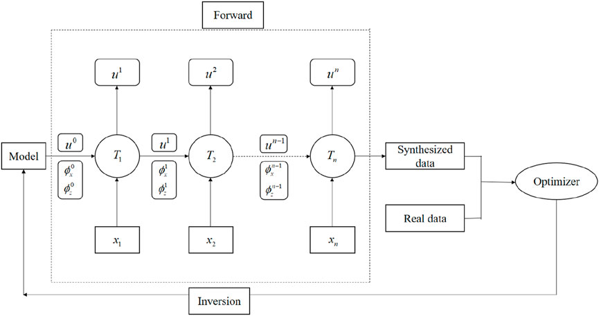
FWI is essentially an optimization problem that aims to minimize the discrepancy between the seismic waveform data recorded by the receiver and the synthetic waveform data generated by forward modeling. Typically, FWI consists of three key components: the forward modeling method, the choice of the loss function, and the selection of the optimizer. In this study, we combine the OSPRK method with an RNN for forward modeling, creating the OSPRK-RNN method for FWI. This approach leverages the similarity between traditional forward modeling algorithms and the computational process of RNNs (Richardson, 2018). Figure 1 illustrates the flowchart for the OSPRK-RNN method for full waveform forward and inverse modeling, where $x_i\left(i=1,2,\cdots ,n\right)$ represents the source data at the moment $T_i$, ${\varphi }_x^i\left(i=0,1,\cdots ,n\right)$ and ${\varphi }_z^i\left(i=0,1,\cdots ,n\right)$ are the auxiliary wavefield information, and $u^i\left(i=1,2\cdots n\right)$ is the output wavefield information. For the forward process in Figure 1, we take the nth moment as an example. By adding the iterative equations of the OSPRK method of PML, $u^n$ at the current moment is determined by the $x_n$ and the $\left(u^{n-1},{\varphi }_x^{n-1},{\varphi }_z^{n-1}\right)$. At the same time, the $\left(u^n,{\varphi }_x^n,{\varphi }_z^n\right)$ can be obtained and used for the next iteration. In this way, $u^n$ (the observed data) can be obtained for each discrete position at each discrete moment. For the inversion process in Figure 1. When the initial velocity model is determined, the computation of the forward method is able to obtain the waveform information at the nth moment. The error between the synthesized waveform information and the real waveform information is calculated by the loss function, and then the initial velocity model is updated using the optimizer in deep learning. When the change in the value of the loss function is smooth, the velocity model at this point is used as the output model.

Figure 1

Figure 1. Full waveform forward and inverse for OSPRK-RNN method.

2.3 Log_Cosh loss function and nadam optimizer

In this paper, we introduce the Log_Cosh loss function and compare its performance in inversion results with that of the MAE and MSE loss functions through numerical experiments (Peng et al., 2022). The Log_Cosh loss function is defined as follows:

$L\left(y,y^p\right)={\displaystyle \sum _{i=1}^n}\ln \left(\cosh \left(y_i-y_i^p\right)\right),$

where $\cosh \left(x\right)=\frac{e^x+e^{-x}}{2}$, $y_i$ is the true value and $y_i^p$ is the predicted value. For smaller $x$, $\log \left(\cosh \left(x\right)\right)$ is approximately equal to $x^2/2$, and for larger $x$, $\ln \left(\cosh \left(x\right)\right)$ is approximately equal to $\left|x\right|-\log \left(2\right)$. This means that the Log_Cosh loss function offers the smoothness of MSE for small prediction errors and the robustness of MAE for larger errors. This adaptive behavior allows the Log_Cosh loss function to better accommodate the data distribution, thereby improving both the accuracy and robustness of the model (Peng et al., 2022; Saleh and Saleh, 2022). In this study, we employ the Nadam optimizer to update the velocity model. The Nadam optimizer is an adaptive learning rate optimization algorithm widely used in deep learning and machine learning tasks. It combines the benefits of the Adaptive Moment Estimation (Adam) optimizer with those of Nesterov Accelerated Gradient (NAG) descent (Dozat, 2016). The Adam optimizer adjusts the learning rate adaptively (Kingma and Ba, 2014), while the NAG method reduces oscillations through predictive updating (Bubeck et al., 2015). This combination allows the Nadam optimizer to effectively address a wide range of complex optimization problems. The update rules for the Nadam optimizer are as follows:

$\left\{\begin{array}{l}{m}_k={\beta }_1{m}_{k-1}+\left(1-{\beta }_1\right)g_k\\ v_k={\beta }_2{v}_{k-1}+\left(1-{\beta }_2\right){g_k}^2\\ {\widehat{m}}_k=\frac{m_k}{1-{{\beta }_1}^k}\\ {\widehat{v}}_k=\frac{m_k}{1-{{\beta }_1}^k}\\ {\overline{m}}_k={\beta }_1{\widehat{m}}_k+\frac{\left(1-{\beta }_1\right)g_k}{1-{{\beta }_1}^k}\\ {\theta }_{k+1}={\theta }_k-\frac{\alpha }{\sqrt{{\widehat{v}}_k}+\epsilon }{\overline{m}}_k\\ m_0=0,v_0=0\end{array}\right.,$

where ${\beta }_1$ and ${\beta }_2$ are the decay coefficients of the two exponentially weighted averages, ${\widehat{m}}_k$ and ${\widehat{v}}_k$ are the bias-corrected moving averages of the gradient terms, ${\theta }_{k+1}$ is the updated model parameter, $\alpha$ is the learning rate, $g_k$ is the gradient of the loss function at step $k$, and $\epsilon$ is a very small constant used to avoid division by zero. In Tensorflow, the default parameters for ${\beta }_1$ and ${\beta }_2$ are 0.9 and 0.999, respectively.

By identifying these three components, we establish a foundational framework for FWI based on deep learning. To further enhance experimental results, we also incorporate additional deep learning techniques, including the use of a small batch strategy, regularization, and grid search for hyperparameter optimization. These techniques help to improve model performance, reduce overfitting, and fine-tune parameters, ultimately leading to more accurate and reliable numerical outcomes.

2.4 Loss function with physical information

In a previous study, Rassi et al. (2019) introduced physical information operators into the loss function to guide the training process, yielding promising results. In this study, we also incorporate physical differential operators into the loss function. Specifically, we define the physical differential operator for the two-dimensional acoustic equation as: $N={\mathrm{\partial }}_{tt}/s^2-{\nabla }^2$ ( ${\nabla }^2=\left(\frac{{\mathrm{\partial }}^2}{\mathrm{\partial }{x}^2}+\frac{{\mathrm{\partial }}^2}{\mathrm{\partial }{z}^2}\right)$. This operator reflects the difference between the predicted and true velocity models. As the velocity model approaches the true model, the value of the differential operator $N$ approaches 0. Based on this, we define the loss function incorporating physical information as follows:

$Loss\left(s\right)={\displaystyle \sum _{t=1}^n}(loss\left(u^t,d^t\right)+N\left(d^t\right))$

where $s$ denotes the speed parameter to be optimized by the model, $d^t$ denotes the real waveform data, and $u^t$ denotes the synthetic waveform data. This loss function will be used to evaluate its effectiveness in the inversion process.

3 Numerical simulation

In this section, we present five numerical experiments to evaluate the effectiveness of combining the OSPRK method with RNN for full waveform forward and inverse modeling. The first experiment demonstrates the accuracy and efficiency of the OSPRK method in forward modeling. The second and third experiments investigate the impact of different loss functions and various Nadam optimizer parameters on FWI performance. In the fourth experiment, we compare the inversion results obtained using the traditional FD method with those from the OSPRK method. Finally, in the fifth experiment, we illustrate the capability of the OSPRK-RNN method in inverting complex velocity models, and we show how the inclusion of physically informed operators significantly improves inversion accuracy.

3.1 Forward modeling of the homogeneous model

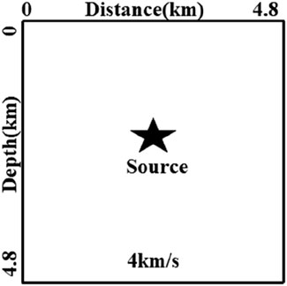
In this numerical experiment, we evaluate the effectiveness of combining the OSPRK method with RNN and compare it to the conventional sixth-order FD method combined with RNN for forward modeling. The computational domain for the homogeneous velocity model is set to 4.8 km × 4.8 km, with a spatial step of $\Delta x$ = $\Delta z$ = 24 m, a time step of $\Delta t$ = 0.001 s, and a velocity of 4,000 m/s. The source is a Ricker wavelet with a peak frequency of 10 Hz, located at the center of the model. Figure 2 shows the model, where a PML is applied as the absorbing boundary condition.

Figure 2

Figure 2. Schematic of the homogeneous velocity model.

We then compare the forward simulation results of the OSPRK method with those of the traditional FD method combined with RNN. As shown in Figure 3, the wavefield snapshot in Figure 3B, obtained using the FD method, displays significant numerical dispersion, whereas the snapshot in Figure 3A, produced by the OSPRK method, exhibits minimal numerical dispersion. Furthermore, the wavefield snapshots in Figures 3C, D confirm that the added PML effectively absorbs boundary-reflected waves as the wave propagates out of the region. In terms of computational efficiency, the time required to compute the entire wavefield is 2.57 s for the OSPRK method and 2.61 s for the conventional FD method. These results demonstrate that the OSPRK method significantly reduces numerical dispersion, while the PML effectively mitigates boundary reflections.

Figure 3

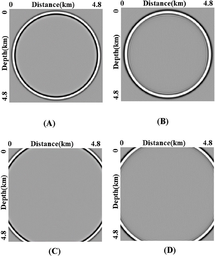
Figure 3. (A, C) and (B, D) Snapshots of the wavefields at t = 0.319 s and t = 0.469 s by OSPRK and FD, respectively.

3.2 Inverse simulation based on a two-layer velocity model

In this experiment, we apply FWI using the OSPRK method combined with RNN, focusing on the effects of three different loss functions and varying learning rates on the inversion results. The two-layer velocity model has a computational domain of 0.25 km × 0.25 km, with a spatial step of $\Delta x$ = $\Delta z$ = 5 m and a time step of $\Delta t$ = 0.001 s. The velocities in Region I and Region II are set to 1800 m/s and 2,400 m/s, respectively. In Figure 4, the black triangle represents the receiver location, and the black pentagram marks the source position. Ricker wavelet sources with a frequency of 10 Hz are located at the bottom of the model and are distributed horizontally across 51 grid points. Receivers are positioned on the surface of the model at 5-meter intervals. In total, there are 51 sources, of which 40 are selected for training, while the remaining 11 are reserved for testing. The mini-batch size is set to 5, and each epoch (defined as a complete pass through the entire training data) consists of 6 iterations. This results in 48 batch iteration steps (one batch iteration step represents one pass through a mini-batch of the training data) for the inversion process.

Figure 4

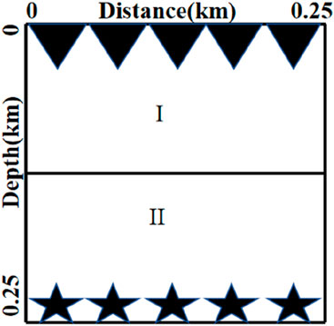
Figure 4. Layered velocity model with [0 km, 0.125 km] × [0 km, 0.25 km] for region I and [0.125 km, 0.25 km] × [0 km, 0.25 km] for region II.

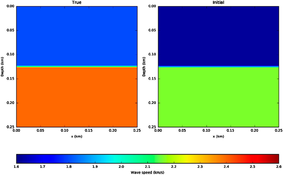
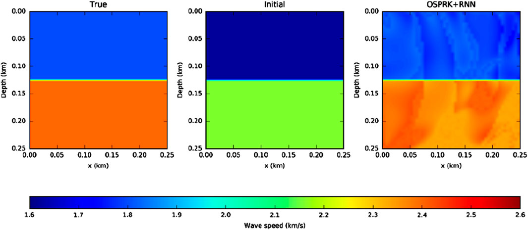
For the initial velocity model used in the inversion, we reduce the velocity by a factor of 0.9. The real velocity model and the initial velocity model are shown in Figure 5. We then perform FWI using three commonly used loss functions—MAE, MSE, and Log_Cosh—across different learning rates. Figure 6 presents the inversion results obtained using these loss functions at learning rates of 10, 20, 30, 50, and 70. Since the magnitudes of the three loss functions differ, we define the relative error $E$ as the $L_1$-norm between the inverted velocity values and the real velocity values at each grid point. Smaller $E$ values indicate a closer match between the inversion results and the true velocity model. The expression for the relative error is given as:

$E=\frac{{\displaystyle \sum _{i=0}^N}{\displaystyle \sum _{j=0}^M}\left|c_{i,j}-c_{i,j}^p\right|}{{\displaystyle \sum _{i=0}^N}{\displaystyle \sum _{j=0}^M}{c}_{i,j}}\times 100\%,$

where N and M are the numbers of rows and columns of the mesh, respectively. $c_{i,j}$ and $c_{i,j}^p$ are the velocities at the ith row and jth column of the mesh point in the inverse velocity model and real velocity model, respectively.

Figure 5

Figure 5. Left: real model; right: initial model.

Figure 6

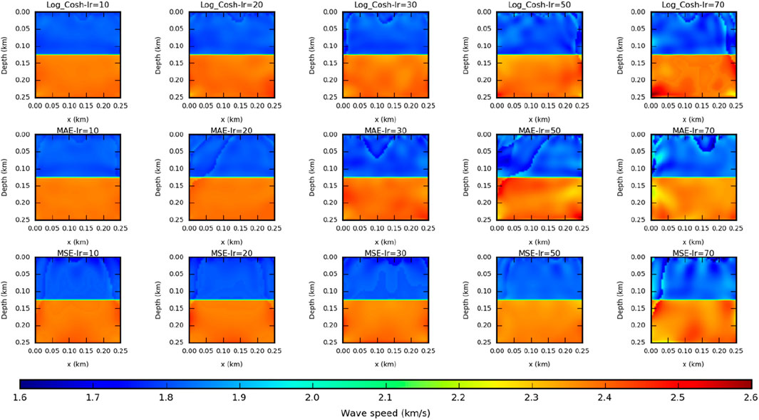
Figure 6. Inversion results obtained by Log_Cosh, MAE, and MSE loss functions at different learning rates.

Table 1 presents the relative errors for the three loss functions at the specified learning rates of 10, 20, 30, 50, and 70. Figure 7 illustrates the line graphs of the relative errors for each loss function across the different learning rates, highlighting the characteristics of each loss function and the influence of learning rates on the inversion results. When $lr\le 30$, the relative errors of the three loss functions show minimal differences, and all yield satisfactory inversion outcomes. However, when $lr\ge 30$, the relative errors for the MAE and MSE loss functions increase significantly, while the relative error for the Log_Cosh loss function rises more gradually. This suggests that the Log_Cosh loss function provides better stability at higher learning rates. Moreover, for all three loss functions, the relative error initially decreases as the learning rate increases, but then begins to rise after surpassing a certain threshold. Based on these observations, it can be concluded that the optimal learning rate for inversion using the OSPRK method falls between 10 and 30.

Table 1

Table 1. Relative error of the three loss functions at five learning rates (%).

Figure 7

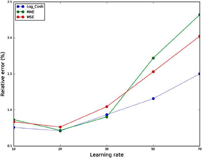
Figure 7. The relative error of the Log_Cosh, MAE, and MSE loss functions at different learning rates in the coordinate system.

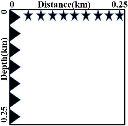
In the following, we will consider the placement of receivers and seismic sources under real full-waveform inversion conditions. We place the receivers vertically every 5 m on the leftmost side of the model area and the sources horizontally every 5 m on the surface, for a total of 51 receivers and 51 sources. Figure 8 shows a schematic diagram of the placement of the seismic sources and receivers.

Figure 8

Figure 8. Schematic diagram of the source and receiver.

In the training process, we choose 40 sources as the training set and the remaining 11 sources are used as the test set. We set the batch size to 3, the learning rate to 20, and the number of traversals to 5, for a total of 65 iterations. As can be seen in Figure 9, the OSPRK method also gives good inversion results in real receiver and seismic source placement scenarios.

Figure 9

Figure 9. Schematic representation of the inversion results.

3.3 Inverse simulation based on the central velocity model

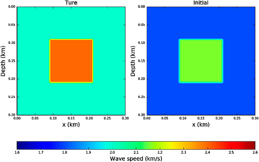
In this experiment, we conduct FWI using the OSPRK method combined with RNN, focusing on the effects of the parameters ${\beta }_1$ and ${\beta }_2$ in the Nadam optimizer on the inversion results. For the central velocity model, the computational domain is set to 0.3 km × 0.3 km, with a spatial step of $\Delta x$ = $\Delta z$ = 6 m and a time step of $\Delta t$ = 0.001 s. The region centered at coordinates [0.09 km, 0.21 km] × [0.09 km, 0.21 km] has a velocity of 2,400 m/s, while the velocity in the surrounding region is 2000 m/s. For the initial velocity model used in the inversion process, we select 0.9 times the real velocity values to generate the starting model. Figure 10 shows a schematic of the initial velocity model versus the actual velocity model.

Figure 10

Figure 10. Schematic diagram of the true and initial velocity models.

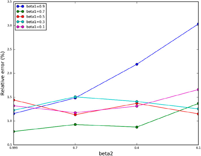
First, the values of the parameters are detailed in Table 2, with β₁ ranging from 0.9 to 0.1 in steps of 0.2, and β₂ ranging from 0.999 to 0.1 in steps of 0.3. This results in a total of 20 sets of inverse numerical simulations.

Table 2

Table 2. Different values of ${\beta }_1$ and ${\beta }_2$.

The Ricker wavelet sources, with a frequency of 10 Hz, are positioned at the bottom of the model and distributed horizontally across 51 grid points. Receivers are placed on the surface of the model at 6-meter intervals. Out of the 51 sources, 39 are selected for training, while the remaining 12 are used for testing. The mini-batch size is set to 3, with an epoch count of 4. This configuration results in a total of 52 batch iteration steps to complete the inversion process. The relative errors for these 20 sets of inverse numerical simulations are displayed in Figure 9.

From Figure 11, it is clear that the default Nadam parameters are not optimal. Among the various parameter configurations, the lowest relative error is achieved with ${\beta }_1=0.7,{\beta }_2>=0.4$. In the following section, we will compare the performance of the loss functions using this optimized parameter configuration (${\beta }_1=0.7,{\beta }_2=0.999$) against the default configuration (${\beta }_1=0.9,{\beta }_2=0.999$).

Figure 11

Figure 11. The relative errors obtained for different values of ${\beta }_1$ and ${\beta }_2$.

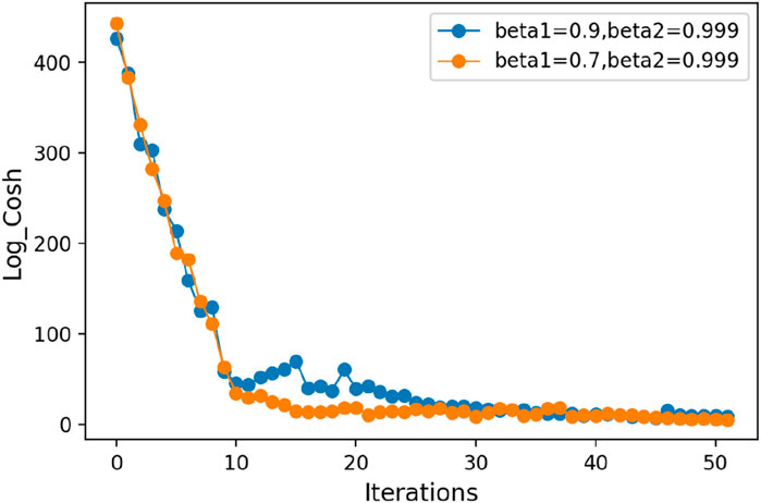
As shown in Figure 12, the loss function curves with the optimized parameters are relatively smooth throughout the descent process and converge after 20 iterations. In contrast, the loss function curves with the default parameters exhibit significant oscillations during the descent process and only converge after 30 iterations.

Figure 12

Figure 12. Loss function comparison between optimized and default parameters.

3.4 Inverse simulation based on a three-layer velocity model

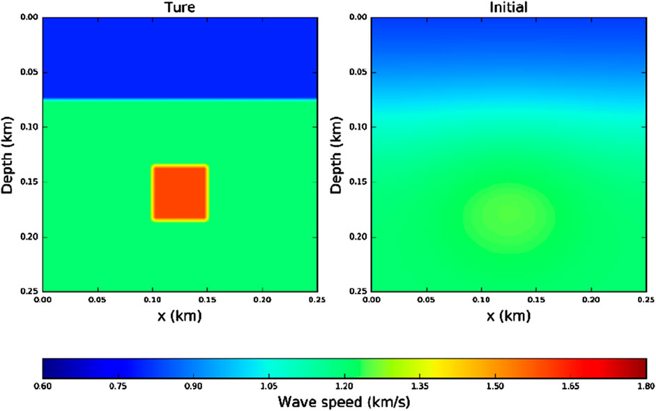
In this experiment, we will use OSPRK-RNN and FD-RNN for full waveform inversion and then compare the inversion results of the two methods. For the three-layer velocity model, the computational domain is 0.25 km × 0.25 km, the spatial step is $\Delta x$ = $\Delta z$ = 5 m, and the time step is $\Delta t$ = 0.001 s. The black triangle in Figure 13 represents the receiver and the black pentagram represents the source. For the locations of receivers and sources, we place receivers horizontally at intervals of 5 m on the ground surface, and we place sources horizontally at intervals of 5 m in a 0.25 km subsurface, with a total of 51 receivers and 51 sources. In the training process, we select 39 sources as the training set and the remaining 12 sources as the test set. For the inversion strategy, we use the Nadam optimizer with optimized parameters and the Log_Cosh loss function with a mini-batch size of 3, an epoch of 5, and a learning rate of 20.

Figure 13

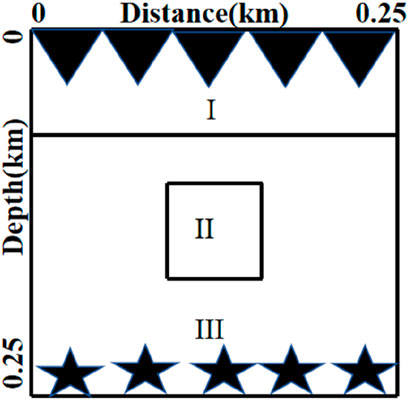
Figure 13. The location of region I is [0 km, 0.075 km] × [0 km, 0.25 km] and the location of region II is [0.14 km, 0.19 km] × [0.1 km, 0.15 km].

For the initial velocity model of the inversion, we choose a Gaussian perturbation of 10% of the true velocity model to generate the initial velocity model. In Figure 14, we give the true velocity model and the initial velocity model. Figure 15 gives a comparison of the inversion between the OSPRK method and the FD method after 65 iterations. From the inversion results in Figure 15, both methods are able to roughly invert the basic shape of the real velocity model. However, the inversion result of the OSPRK method is closer to the real velocity model in terms of the dividing line between regions I and III and the shape of region II. For the relative errors of the velocity model after inversion, the relative errors of the OSPRK method and the FD method are 1.275% and 2.137%, respectively. As a result, our proposed OSPRK will be more accurate than the FD method in the inversion results.

Figure 14

Figure 14. Real velocity model and initial velocity model for three-layer media.

Figure 15

Figure 15. Comparison of the inversion results of the FD method with the OSPRK method.

3.5 Inverse simulation based on complex sigsbee model

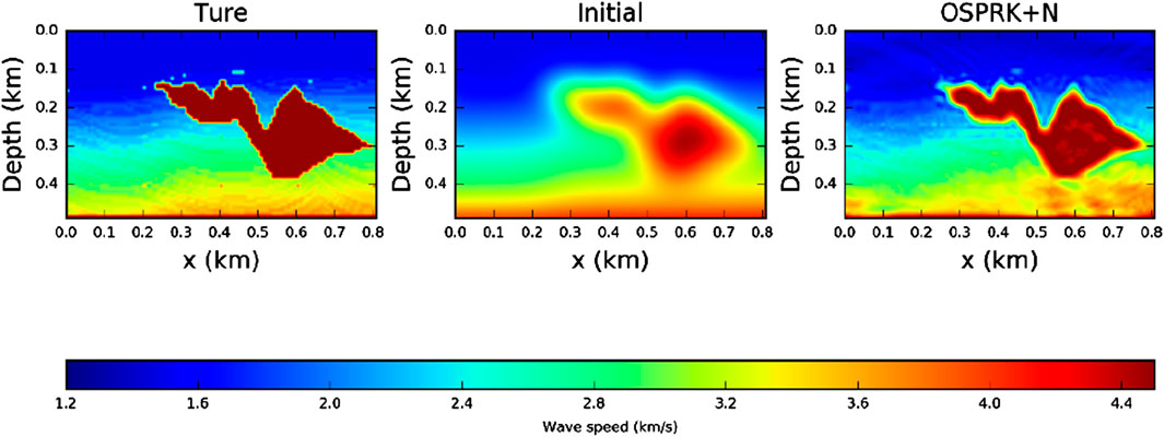
In the final numerical experiment, we perform an inversion on a complex Sigsbee velocity model. The computational domain is 0.488 km × 0.808 km, with velocities ranging from 1,400 m/s to 4,500 m/s. The model features a high-velocity anomaly of 4,500 m/s in the central region. The spatial step is $\Delta x$ = $\Delta z$ = 8 m, and the time step is $\Delta t$ = 0.001 s. Ricker wavelet sources with a frequency of 10 Hz are placed at the bottom of the model and distributed horizontally across 101 grid points. Receivers are located on the surface of the model at 8-meter intervals. Of the 101 sources, 80 are used for training, while the remaining 21 are reserved for testing. The learning rate is set to 30, the mini-batch size is 5, and each epoch consists of 10 iterations, resulting in a total of 160 batch iteration steps for the inversion process.

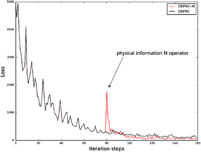
For the first 80 iterations, we use only the data information in the loss function. In the last 80 iterations, we incorporate physical information into the loss function. As shown in Figure 16, the value of the loss function with physical information added during the final 80 iterations is significantly lower than that of the loss function without physical information. This demonstrates that incorporating physical information into the loss function enhances the inversion accuracy. Figure 17 shows that the OSPRK method, when augmented with physical information, successfully inverts the high-velocity anomalies, indicating that this approach is highly effective for inverting complex velocity models.

Figure 16

Figure 16. Loss function decline curves with and without physical information added.

Figure 17

Figure 17. Inversion results of the OSPRK method with added physical information.

4 Conclusion

In this study, we combined the OSPRK forward modeling method with an RNN for full waveform forward and inverse modeling. Additionally, we introduced the Log_Cosh loss function and the Nadam optimizer from deep learning, conducting one forward modeling and four inverse numerical simulations to demonstrate the effectiveness of our approach. The first experiment, which involved uniform medium forward modeling, showed that the OSPRK method effectively suppresses numerical dispersion compared to the conventional FD method. In the second experiment, using a two-layer velocity model for inversion, we confirmed that the Log_Cosh loss function offers greater stability across various learning rates compared to MSE and MAE. The third experiment, which focused on a central velocity model, demonstrated that optimized Nadam parameters result in faster convergence and higher inversion accuracy compared to default settings. The fourth experiment revealed that the OSPRK method yields more accurate inversion results than the FD method. Finally, in the inversion of a complex Sigsbee velocity model, we utilized an optimized Nadam optimizer and a loss function incorporating physical operators, highlighting the high efficacy of combining deep learning techniques with the OSPRK method. All these numerical simulations are based on the acoustic wave equation, a simplified mathematical-physical model of seismic wave propagation. In future research, we plan to integrate deep learning techniques with more complex elastic wave equations. Additionally, since the RNN framework may face challenges such as gradient vanishing and explosion, another key focus of our future work will be exploring neural network frameworks with improved performance.

Data availability statement

The original contributions presented in the study are included in the article/supplementary material, further inquiries can be directed to the corresponding author.

Author contributions

YZ: Writing–review and editing. XL: Methodology, Validation, Writing–original draft, Writing–review and editing. XuH: Writing–review and editing. XiH: Writing–review and editing. TC: Writing–review and editing.

Funding

The author(s) declare that financial support was received for the research, authorship, and/or publication of this article. This work was supported by the National Natural Science Foundation of China under Grant 42330801, and Grant 42374143.

Acknowledgments

We thank Alan Richardson for providing his open-source code at https://arxiv.org/abs/1801.07232. His code provides an important basis for the progress of this study.

Conflict of interest

The authors declare that the research was conducted in the absence of any commercial or financial relationships that could be construed as a potential conflict of interest.

Publisher’s note

All claims expressed in this article are solely those of the authors and do not necessarily represent those of their affiliated organizations, or those of the publisher, the editors and the reviewers. Any product that may be evaluated in this article, or claim that may be made by its manufacturer, is not guaranteed or endorsed by the publisher.

References

Bubeck, S., Lee, Y. T., and Singh, M. (2015). A geometric alternative to nesterov's accelerated gradient descent. Mathematics. doi:10.48550/arXiv.1506.08187

CrossRef Full Text | Google Scholar

Dozat, T. (2016). Incorporating nesterov momentum into Adam.

Google Scholar

Eriksson, K., and Johnson, C. (1991). Adaptive finite element methods for parabolic problems. I.: a linear model problem. Soc. Industrial Appl. Math. 28, 43–77. doi:10.1137/0728003

CrossRef Full Text | Google Scholar

Feng, K., and Qin, M. (2010). Symplectic geometric algorithms for Hamiltonian systems. Germany: Springer. doi:10.1007/978-3-642-01777-3

CrossRef Full Text | Google Scholar

Kingma, D., and Ba, J. (2014). Adam: a method for stochastic optimization. Comput. Sci. doi:10.48550/arXiv.1412.6980

CrossRef Full Text | Google Scholar

Kirkpatrick, S., Gelatt, C. D., and Vecchi, M. P. (1983). Optimization by simulated annealing. Science 220, 671–680. doi:10.1126/science.220.4598.671

PubMed Abstract | CrossRef Full Text | Google Scholar

Li, Y. Y., Alkhalifah, T., Huang, J., and Li, Z. (2023). Self-supervised pretraining vision transformer with masked autoencoders for building subsurface model. Trans. Geoscience Remote Sens. 6, 11–10. doi:10.1109/TGRS.2023.3308999

CrossRef Full Text | Google Scholar

Li, Y. Y., Alkhalifah, T., and Zhang, Z. (2021). Deep-learning assisted regularized elastic full waveform inversion using the velocity distribution information from wells. Geophys. J. Int. 226, 1322–1335. doi:10.1093/gji/ggab162

CrossRef Full Text | Google Scholar

Liu, S. L., Yang, D. H., and Ma, J. (2017). A modified symplectic PRK scheme for seismic wave modeling. Comput. and Geosciences 99, 28–36. doi:10.1016/j.cageo.2016.11.001

CrossRef Full Text | Google Scholar

Lu, F., Zhou, Y. J., He, X. J., Ma, X., and Huang, X. Y. (2021). Full waveform inversion based on deep learning and optimal nearly analytic discrete method. Appl. Geophys. 18 (4), 483–498. doi:10.1007/s11770-021-0912-4

CrossRef Full Text | Google Scholar

Ma, S., Li, D., Hu, T., Xing, Y., and Nai, W. (2020). Huber loss function based on variable step beetle antennae search algorithm with Gaussian direction. Int. Conf. Intelligent Human-Machine Syst. Cybern. (IHMSC) 1, 248–251. doi:10.1109/IHMSC49165.2020.00062

CrossRef Full Text | Google Scholar

Ma, X., and Yang, D. H. (2017). A phase-preserving and low-dispersive symplectic partitioned Runge-Kutta method for solving seismic wave equations. Geophys. J. Int. 209, 1534–1557. doi:10.1093/gji/ggx097

CrossRef Full Text | Google Scholar

Moczo, P., Kristek, J., Vavrycuk, V., Archuleta, R. J., and Halada, L. (2002). 3d heterogeneous staggered-grid finite-difference modeling of seismic motion with volume harmonic and arithmetic averaging of elastic moduli and densities. Bull. Seismol. Soc. Am. 92 (8), 3042–3066. doi:10.1785/0120010167

CrossRef Full Text | Google Scholar

Peng, K., Guo, H. Y., and Shang, X. Y. (2022). Microseismic source location using the Log-Cosh function and distant sensor-removed P-wave arrival data. J. Central South Univ. 29 (2), 712–725. doi:10.1007/s11771-022-4943-7

CrossRef Full Text | Google Scholar

Qin, M. Z., and Zhang, M. Q. (1990). Multi-stage symplectic schemes of two kinds of Hamiltonian systems for wave equations. Comput. Math. Appl. 19 (10), 51–62. doi:10.1016/0898-1221(90)90357-P

CrossRef Full Text | Google Scholar

Raissi, M., Perdikaris, P., and Karniadakis, G. E. (2019). Physics-informed neural networks: a deep learning framework for solving forward and inverse problems involving nonlinear partial differential equations. J. Comput. Phys. 378, 686–707. doi:10.1016/j.jcp.2018.10.045

CrossRef Full Text | Google Scholar

Richardson, A. (2018). Seismic full-waveform inversion using deep learning tools and techniques. doi:10.48550/arXiv.1801.07232

CrossRef Full Text | Google Scholar

Saenger, E. H., Krüger, O. S., and Shapiro, S. A. (2004). Effective elastic properties of randomly fractured soils: 3d numerical experiments. Geophys. Prospect. 52 (3), 183–195. doi:10.1111/j.1365-2478.2004.00407.x

CrossRef Full Text | Google Scholar

Saleh, R. A., and Saleh, A. K. M. E. (2022). Statistical properties of the Log_Cosh loss function used in machine learning. Arxiv. doi:10.48550/arXiv.2208.04564

CrossRef Full Text | Google Scholar

Song, C., and Alkhalifah, T. (2021). Wavefield reconstruction inversion via physics-informed neural networks. IEEE Trans. Geoscience Remote Sens. 60, 1–12. doi:10.1109/TGRS.2021.3123122

CrossRef Full Text | Google Scholar

Tarantola, A. (1984). Inversion of seismic reflection data in the acoustic approximation. Geophysics 49 (8), 1259–1266. doi:10.1190/1.1441754

CrossRef Full Text | Google Scholar

Tong, P., Zhao, D., Yang, D. H., Liu, Q., and Chen, J. (2014). Wave-equation based traveltime seismic tomography – part 1: method. Solid Earth Discuss. 6 (2), 2523–2566. doi:10.5194/sed-6-2523-2014

CrossRef Full Text | Google Scholar

Virieux, J. (1986). P-sv wave propagation in heterogeneous media velocity-stress finite-difference method. Geophysics 51, 889–901. doi:10.1190/1.1442147

CrossRef Full Text | Google Scholar

Virieux, J., and Operto, S. (2009). An overview of full-waveform inversion in exploration geophysics. Geophysics 74 (6), WCC1–WCC26. doi:10.1190/1.3238367

CrossRef Full Text | Google Scholar

Wang, S. D. (2003). Absorbing boundary condition for acoustic wave equation by perfectly matched layer. Oil Geophys. Prospect. 38 (1), 31–34. doi:10.1007/BF02873153

CrossRef Full Text | Google Scholar

Wu, Y. L., and McMechan, G. A. (2019). Parametric convolutional neural network-domain full-waveform inversion. Geophysics 84 (6), R881–R896. doi:10.1190/geo2018-0224.1

CrossRef Full Text | Google Scholar

Wu, Z. D., and Alkhalifah, T. (2014). The optimized expansion based low-rank method for wavefield extrapolation. Geophysics 79 (2), T51–T60. doi:10.1190/GEO2013-0174.1

CrossRef Full Text | Google Scholar

Wu, Z. D., and Alkhalifah, T. (2018). A highly accurate finite-difference method with minimum dispersion error for solving the Helmholtz equation. J. Comput. Phys. 365, 350–361. doi:10.1016/j.jcp.2018.03.046

CrossRef Full Text | Google Scholar

Yang, D. H., Liu, E., and Zhang, Z. (2008). Evaluation of the u-W finite method in anisotropic porous media. J. Seismic Explor. 17 (2-3), 273–299. doi:10.1093/petrology/egn007

CrossRef Full Text | Google Scholar

Yang, D. H., Peng, J. M., Lu, M., and Terlaky, T. (2006). Optimal nearly analytic discrete approximation to the scalar wave equation. Bull. Seismol. Soc. Am. 96, 1114–1130. doi:10.1785/0120050080

CrossRef Full Text | Google Scholar

Yang, D. H., Teng, J., Zhang, Z., and Liu, E. (2003). A nearly analytic discrete method for acoustic and elastic wave equations in anisotropic media. Bull. Seismol. Soc. Am. 93 (2), 882–890. doi:10.1785/0120020125

CrossRef Full Text | Google Scholar

Zhang, J. H., and Yao, Z. X. (2013). Optimized explicit finite-difference schemes for spatial derivatives using maximum norm. J. Comput. Phys. 250, 511–526. doi:10.1016/j.jcp.2013.04.029

CrossRef Full Text | Google Scholar