Comparison of ECHAM6-wiso near-surface water vapour isotopic composition with in situ measurements at Neumayer Station III

Water isotope records from polar ice cores are crucial proxies for reconstructing past Antarctic climate and temperature changes. For such task, a robust understanding and accurate quantification of the temporal changes between ${\delta }^{18}O$ and temperature is necessary. One option to facilitate this is employing simulations from atmospheric general circulation models that incorporate stable water isotopes. In this context, we assess in this study the results of the isotope-enabled AGCM ECHAM6-wiso model. We analyse results from a high-resolution simulation covering the period 2017–2020, where the atmospheric dynamics is nudged to ERA5 reanalysis data from the European Centre for Medium-Range Weather Forecasts (ECMWF). Our investigation evaluates the agreement between different observed and simulated key physical and isotope quantities, including temperature, humidity, and the isotopic composition of surface water vapour (${\delta }^{18}{O}_v$ and $\delta D_v$), at Neumayer Station III in East Antarctica. Additionally, our study evaluates the skill of the ECHAM6-wiso model in simulating stable water isotope ratios in snow (${\delta }^{18}{O}_{\mathit{snow}}$ and $\delta D_{\mathit{snow}}$) at Neumayer Station III for the recent past. The ECHAM6-wiso model exhibits skill in replicating the daily, monthly, and seasonal fluctuations of temperature, humidity, surface water vapour ${\delta }^{18}{O}_v$, and $\delta D_v$. However, it demonstrates limitations in accurately simulating d-excess values on the different time scales. While the model does not precisely reproduce the observed surface ${\delta }^{18}{O}_v$-temperature relationship on a daily scale, it closely approximates this relationship on a monthly scale. For snow, the model slightly underestimates the ${\delta }^{18}{O}_{\mathit{snow}}$-temperature relationship when compared to observational data. To test if the ECHAM6-wiso model correctly simulates the water vapour sources and transport pathways to Neumayer Station III, we have performed related back trajectory studies. Based on simulation results of the FLEXPART model, we find that the water vapour back-trajectory results with ECHAM6-wiso are consistent with those based on ERA5 data. This result leads to the conclusion that ECHAM6-wiso is a very useful tool for analysing atmospheric moisture sources and transport pathways to East Antarctica under present climate conditions.

1 Introduction

Temperature is a critical variable for understanding the Earth’s climate system, discerning climatic patterns, and investigating climatic changes. A predominant technique for inferring historical temperature fluctuations is the analysis of water stable isotopes in ice cores, which can be used as a reliable climate indicator (Dansgaard, 1964; Lorius and Merlivat, 1975). To this end, ${\delta }^{18}O$ and $\delta D$ measurements in polar ice cores have been used in numerous studies for reconstructing temperature variations over glacial and interglacial periods (e.g., Jouzel et al., 2007; NEEM community members, 2013). For such reconstructions a linear relationship between past temperature and water stable isotope changes, which are preserved in ice cores, was previously assumed (e.g., Petit et al., 1999). However, the previous assumption that the contemporary spatial temperature-isotope relation mirrors the temporal relation required for past temperature reconstructions is currently being questioned. It is now widely accepted that such relation is not universally applicable, and different temporal temperature-isotope gradients have been suggested for climate changes at different ice core drilling sites in East Antarctica (e.g., Sime et al., 2009; Buizert et al., 2021; Kino et al., 2021; Cauquoin et al., 2023; Casado et al., 2023).

For the principal understanding of water isotope changes in relation to different climate quantities, measurements of water stable isotopes in precipitation and water vapour have been systematically conducted since the 1950s (Dansgaard, 1953). These measurements have been proven pivotal for characterizing and comprehending the atmospheric hydrological cycle and the usage of stable water isotopes as a paleothermometer (e.g., Yoshimura, 2015; Galewsky et al., 2016). The stable water isotopic composition of both precipitation and vapour, altered by isotopic fractionation during water phase transitions, is a cumulative record of the physical processes within the atmospheric hydrological cycle. The fractionation coefficients and molecular diffusivities of individual water stable isotopes have been quantified through laboratory experiments concerning ice-vapour exchange and liquid-vapour exchange (Merlivat and Nief, 1967; Barkan and Luz, 2007; Ellehoj et al., 2013). Subsequent theoretical work has yielded isotopic exchange parameterizations for processes like precipitation, snow crystal formation, ocean evaporation and supersaturation under very cold conditions (Stewart, 1975; Jouzel and Merlivat, 1984; Bolot et al., 2013; Merlivat and Jouzel, 1979; Wang and Yakir, 2000). Despite this gain of knowledge on the microphysical scale, the calibration of an isotopic paleothermometer is still complex, though, due to many influencing factors on a larger macrophysical scale. For Antarctica, key factors include the variability in temperature inversion strength, the seasonality and intermittency of snowfall, changes in the elevation of glacial ice sheets, sea ice coverage, and alterations in moisture sourcing and transport to Antarctica (Masson-Delmotte et al., 2011; Sime et al., 2013; Werner et al., 2018; Kino et al., 2021; Casado et al., 2023; Cauquoin et al., 2023).

An alternative option to improve the calibration of an isotopic paleothermometer is to utilise general circulation models (GCMs) with explicit diagnostics of water stable isotopes, so-called isotope-enabled GCMs. These models offer a mechanistic understanding of the physical processes influencing the isotopic composition of different water bodies in the climate system. They permit the explicit simulation of isotopic fractionation processes during any phase changes in a water mass within the model’s hydrological cycle. Examples of such processes include evaporation of water from the land or ocean surface, cloud droplet formation, and re-evaporation of droplet water below the cloud base. In such an isotope-enabled GCM, all the relevant factors determining the strength and variability of isotopic fractionation are known. Since the pioneering work of Joussaume et al. (1984), several isotope-enabled GCMs have been built for the atmosphere, such as LMDZiso (Risi et al., 2010), ECHAM5-wiso (Werner et al., 2011), isoGSM (Yoshimura and Kanamitsu, 2008), iCAM5 (Nusbaumer et al., 2017), MIROC5-iso (Okazaki and Yoshimura, 2019) and ECHAM6-wiso (Cauquoin et al., 2019; Cauquoin and Werner, 2021). These models are extremely helpful because they enable a direct comparison between measured and modelled isotope values and can reduce the uncertainties that exist in interpreting measured isotope values in terms of past temperature changes.

To evaluate the accuracy of these isotope-enabled models, a robust comparison with ice core records and present-day isotope measurements is imperative. During the last decade, isotope-enabled models have been thoroughly assessed through several comparisons of observed and simulated isotopic compositions in precipitation within different Arctic and Antarctic regions (e.g., Steen-Larsen et al., 2011; Masson-Delmotte et al., 2015; Goursaud et al., 2018). These comparisons, however, are constrained by the timing and duration of precipitation events and might not fully cover the models’ response to swift meteorological changes (Kino et al., 2021). Moreover, recent research, including studies conducted in Greenland (Steen-Larsen et al., 2014; Steen-Larsen et al., 2013; Madsen et al., 2019) and Antarctica (Casado et al., 2018; Ritter et al., 2016) and by wind tunnel experiments (Ebner et al., 2017; Wahl et al., 2024), has provided insights into isotopic exchanges between surface snow and the overlying vapour. These studies suggest the occurrence of post-depositional effects, which implies that the isotopic changes in ice cores might represent a continuous record of paleoclimatic changes, even during dry intervals without precipitation events. Such findings indicate that comparisons between measured isotope changes in snow or ice and isoAGCM simulation values of isotope changes in Antarctic precipitation might be biased if isotopic exchanges between snow and water vapour are neglected in these simulations.

In addition, the interpretation of the water isotope records in the Antarctic coastal zone is more difficult because distillation is not the only dominant influence on the water isotope signal. Local effects, such as ocean evaporation influenced by the presence of sea ice, katabatic wind direction and speed, surface snow remobilization, sublimation, and wind-blown snow metamorphism can significantly impact the isotopic composition of deposited snow and, consequently, the archived signal (Ekaykin et al., 2002; Casado et al., 2018). For an improved model assessment it is therefore necessary to extend the existing evaluations of isoAGCM results to the isotopic composition of water vapour (Ollivier et al., 2025).

In this study, we compare the simulated isotopic composition of water vapour of the isotope-enabled AGCM ECHAM6-wiso with in-situ measurements of isotope changes in surface water vapour at Neumayer Station III in Antarctica. Continuous water vapour isotope measurements have been performed over 3 years at this location. This comparative analysis allows for an evaluation of the model’s ability to accurately represent stable water isotopes in near-surface water vapour. To link the results of analysed isotope changes in near-surface vapour with isotope changes in surface snow, the study also compares the modeled water stable isotope changes in snowfall at Neumayer Station with observational data from two recent decades.

The main aims of this study include: (i) assessing the performance of ECHAM6-wiso in modelling water vapour and precipitation at the coastal Antarctic location of Neumayer III Station; (ii) evaluating the ability of the ECHAM6-wiso model to simulate the primary transport pathways and source regions of water reaching Neumayer Station; (iii) investigating the correlation between simulated meteorological and isotopic variables in water vapour and their relationship with observed precipitation, and determining the agreement of the model results with prior findings on the temperature–${\delta }^{18}O$ and ${\delta }^{18}O$–$\delta D$ gradients in surface snow and water vapour at Neumayer Station; and (iv) comparing the results of a nudged versus non-nudged ECHAM6-wiso simulation setup.

2 Methods and data

2.1 The study site: Neumayer Station III

Neumayer Station III (hereinafter also referred to simply as Neumayer Station), a German research base operated by the Alfred Wegener Institute (AWI), Helmholtz Centre for Polar and Marine Research, stands at coordinates 70°40S, 8°16′W in Antarctica. Since 1981, AWI has been conducting continuous meteorological and glaciological observations in this region, initially at the original Georg-von-Neumayer Station located at 70°37′S, 8°22′W until March 1992, followed by operations at Neumayer Station II at 70°39′S, 8°15′W, and transitioning to the current Neumayer Station III in February 2009 (König-Langlo and Loose, 2007). Placed atop the 200-meter-thick Ekström Ice Shelf, approximately 42 m above sea level, Neumayer Station III is characterized by a uniform, gently southward-sloping terrain. The flowing Ekström Ice Shelf, exhibiting a significant thickness gradient towards its grounding line, changes the location of the station at a pace of approximately 200 m annually towards the northern open sea, about 16 km from the station, with the nearest edge of the ice shelf lying 6.2 km to the east-northeast (König-Langlo and Loose, 2007). Seasonally, the sea ice around the station reaches its minimum extent in February and peaks in September, with the coastal regions becoming partially ice-free during the summer months (König-Langlo and Loose, 2007).

Like many coastal Antarctic stations, the climatic conditions at Neumayer Station are dominated by high-velocity winds averaging 8.7 m/s annually, with daily values oscillating by an average of $\pm$ 5.7 m/s. These winds, which are characterized by strong variations in both speed and direction, are an expression of complicated dynamical processes that are influenced by transient cyclones and katabatic air flows near the station (Kottmeier and Fay, 1998). There are two primary wind directions observed at Neumayer Station: the predominant easterlies, driven by cyclonic systems migrating eastward above the Antarctic coastal zone within the circumpolar trough, and the less frequent southerly to south-westerly winds, which arise from a combination of damped katabatic winds and synoptic patterns, typically having speeds under 10 m/s (König-Langlo and Loose, 2007; Rimbu et al., 2014).

Snowfall at the Neumayer Station is often accompanied by strong winds that mobilize and elevate ground snow, resulting in a turbulent mix of fresh precipitation and re-entrained surface snow, termed blowing snow (Schlosser, 1999). The initiation of drifting or blowing snow events at Neumayer Station is sensitive to the prevailing snow surface conditions, typically occurring when wind speeds reach between 6 and 12 m/s. These phenomena are noted in 40% of all visual meteorological recordings (König-Langlo and Loose, 2007). Direct measurement of precipitation is complicated by such pervasive influence of drifting and blowing snow, necessitating glaciological methods to estimate mean annual accumulation, which is estimated as approximately 340 mm w. e. (water equivalent) per year. Since the onset of temperature recordings in 1981, the mean annual near-surface air temperature at Neumayer Station has been maintained at −16.1 °C, with a 1-sigma standard deviation of $\pm$ 1.1 °C for annual mean temperatures over the period until 2018, with no discernible long-term trend in air temperature being detected (Medley et al., 2018).

2.2 Meteorological and isotope measurements at Neumayer Station

Meteorological data for this study were taken from the routinely collected weather station data at Neumayer Station, with the instrumentation positioned 50 m from the main structures of the station and 2 m above the ground surface. The data used include hourly mean atmospheric temperature, relative humidity, and barometric pressure throughout the study period, which spanned from February 2017 to January 2020 (Schmithüsen et al., 2019; Schmithüsen and Jörss, 2021).

The isotopic composition of water vapour was monitored using a high-precision laser spectrometer, with air samples drawn from an inlet situated on the station’s roof, at an elevation of 24 m. For this task, Neumayer Station was equipped with a Picarro L2140-i isotope analyzer in January 2017, enabling continuous monitoring of atmospheric water vapour isotopic ratios. The initial 2 years of water vapour isotope data, covering the period from February 2017 to January 2019, were already documented by Bagheri Dastgerdi et al. (2021). This study extends the dataset by adding an additional year of observations, covering the period from February 2019 to January 2020. Calibration of the isotopic measurements followed the protocol described by Bagheri Dastgerdi et al. (2021), addressing four main challenges specific to the polar environment of Neumayer Station:

Low Humidity Issues: The Picarro instrument is specified by the manufacturer to operate optimally within a humidity range of 1,000 ppm–50,000 ppm, equivalent to a specific humidity of 0.6–31.1 g/kg. However, during the austral winter, the humidity at Neumayer station often falls below this range. To mitigate systematic errors arising from these dry conditions, a humidity response correction was applied to measurements when water vapour concentrations were below 2000 ppm (1.2 g/kg).

Instrumental Drifts: Over time, or subsequent to each restart, the spectrometer is susceptible to various forms of drift. The calibration protocol includes adjustments for such potential long-term instrumental drifts.

Offsets: Discrepancies between the isotopic ratios measured by the Picarro instrument and the actual values, which are determined with higher precision in a laboratory setting, were corrected through the application of an offset adjustment.

Extraneous Data: The calibration routine also incorporates a filtration system that flags and excludes data from periods when measurements might be compromised, such as instances when station exhaust gases could contaminate vapour samples, or during technical malfunctions.

Taking all these effects into account, the post-calibration precision of the Picarro isotopic measurements across the duration of the observational period is quantified as having a mean uncertainty of 0.4‰for ${\delta }^{18}{O}_v$, 3.0‰for $\delta D_v$, and 3.0‰for $d_v$ values. This level of uncertainty accounts for the combined influence of the enumerated corrective measures on the data integrity, ensuring the reliability of the isotopic composition results derived from this study (for details see Bagheri Dastgerdi et al., 2021).

2.3 ECHAM-wiso model description

The ECHAM model is an advanced atmospheric general circulation model (GCM) developed at the Max Planck Institute for Meteorology. Originally derived from the ECMWF weather prediction model, it has undergone substantial evolution, incorporating sophisticated parameterizations for atmospheric dynamics, radiation, cloud microphysics, and hydrology. The ECHAM model employs a spectral-transform dynamical core to solve the primitive equations governing atmospheric motion. It consists of a dry hydrostatic spectral model for advection and pressure tendencies, as well as a semi-Lagrangian transport model for non-dynamic quantities such as moisture (Lin and Rood, 1996). Cloud processes are simulated using a two-moment microphysics scheme, differentiating between liquid, ice, and mixed-phase clouds (Mauritsen et al., 2019). The most recent version, ECHAM6, includes significant improvements in radiative transfer, convection schemes, and cloud formation as compared to the previous model release ECHAM5 (Stevens et al., 2013).

A major enhancement to the ECHAM model is the explicit incorporation of the two stable water isotopes ($H_2^{16}O$, $H{D}^{16}O$, and $H_2^{18}O$), which serve as tracers for hydrological and climatic processes (Werner et al., 2011; Cauquoin et al., 2019). Within the model framework, water isotopes are treated similarly to their standard $H_{2}O$ counterparts, except during phase transitions, such as condensation, evaporation, and sublimation, as well as supersaturation effects during freezing processes at very low temperatures, where isotopic fractionation processes occur. These processes lead to isotopic equilibrium or disequilibrium, depending on the rate of phase change, with kinetic fractionation processes also taken into account (IAEA, 1998). The transport of both ordinary water and isotopic variants is independently modeled across all phases - vapour, liquid, and ice - using the ECHAM flux-form semi-Lagrangian transport scheme (Lin and Rood, 1996). This isotope-enabled variant of the ECHAM model, which has been labelled as ECHAM5-wiso and ECHAM6-wiso respectively, enables the simulation of isotopic compositions across various hydrological reservoirs, providing an improved understanding of isotope variations both in the modern hydrological cycle and related to paleoclimate changes. Both ECHAM5-wiso and ECHAM6-wiso have been applied in numerous model-data comparison studies, such as Antarctica, Siberia, and Greenland (e.g., Goursaud et al., 2018; Butzin et al., 2014; Steen-Larsen et al., 2017; Dietrich et al., 2023; Dreossi et al., 2024) and have contributed to various paleoclimate research studies (Werner et al., 2018; Cauquoin et al., 2023).

The ECHAM6-wiso model is typically configured with a spectral resolution of T63 (approximately $1.9°\times 1.9°$) or T127 (approximately $0.94°\times 0.94°$), with 47 or 95 vertical levels extending into the stratosphere. Higher spatial resolutions (T127L95) yield improved temperature and precipitation patterns, and a more realistic representation of cloud cover and topographic influences. Simulated values of d18O and dD are also in better agreement with various observations for a higher spatial ECHAM model resolution (Werner et al., 2011; Cauquoin and Werner, 2021).

To align simulated atmospheric circulation with observations, the ECHAM6-wiso model in this study was nudged to the ERA5 reanalysis datasets (Hersbach et al., 2020). In this case, modeled three-dimensional fields of temperature, vorticity, and divergence, as well as surface pressure, were nudged every 6 hours towards the reanalysis data (Rast et al., 2013). In contrast to the atmospheric flow, the hydrological cycle and its isotopic variations is still fully prognostic and not nudged to any reanalysis data.

For analysing the dependency of ECHAM6-wiso model results on prescribed boundary conditions (see Chapter 4.5 below), we compare this ECHAM6-wiso simulation to a previously performed ECHAM5-wiso simulation (Werner et al., 2011). This ECHAM5-wiso simulation was run with a spatial resolution of T106L31, corresponding to a horizontal grid size of approximately 1.1$◦$ $\times$ 1.1$◦$, and included 31 vertical levels from the surface to the top of the atmosphere. It was nudged to the older ERA-interim reanalysis data set (Dee et al., 2011). Both setups for ECHAM5-wiso and ECHAM6-wiso, including the applied nudging technique to the different ECMWF reanalyses data sets, are described in detail in Cauquoin and Werner (2021).

2.4 Moisture source diagnostics

Back trajectory models trace air parcels arriving at specific locations. By incorporating meteorological data into such models, it becomes possible to identify key evaporation areas, which serve as origins for water vapour, and water vapour transport pathways. Both are primary factors influencing the isotopic composition of the water vapour (${\delta }^{18}{O}_v$, $\delta D_v$, and $d_v$) at a final target location.

The Lagrangian particle dispersion model FLEXPART, as described by (Brioude et al., 2013), possesses the capability to simulate the back trajectories of air masses, tracing the pathways and origins of atmospheric flow. Coupled with a Lagrangian moisture source diagnostic (Sodemann et al., 2008), FLEXPART is capable of analyzing the provenance of moisture arriving at specific locations by monitoring the variations in humidity content along simulated back trajectories.

Bagheri Dastgerdi et al. (2021) utilized the FLEXPART model, enhanced by the Lagrangian moisture source diagnostic, to investigate seasonal differences in the main moisture uptake areas for vapour transported to Neumayer Station. For this task, Bagheri Dastgerdi et al. (2021) used the ERA5 reanalysis dataset (Hersbach et al., 2020) to derive the forcing data for the FLEXPART model.

This research study explores the potential of using ECHAM6-wiso as an alternative data source for the FLEXPART model. To achieve this, we compare FLEXPART results obtained using two different input datasets: one based on the ERA5 reanalysis dataset and the other one utilizing ECHAM6-wiso simulation results. This approach is employed in our study to investigate two primary aspects: firstly, to identify the source regions and transport pathways of water vapour reaching Neumayer Station for the investigated 3-year observation period between February 2017 and January 2020; and secondly, to evaluate the ability of the ECHAM6 model in simulating the same water vapour sources and transfer pathways as identified for the ERA5 forcing data.

The FLEXPART model requires a comprehensive set of meteorological forcing data across all vertical layers (61 in total), including horizontal wind components (U and V) in $m{s}^{-1}$, vertical velocity in $Pa{s}^{-1}$, temperature in K, surface pressure in Pa, and specific humidity in $kgk{g}^{-1}$. Additionally, it requires a suite of surface variables, such as snow depth data in meters of water equivalent mean sea level pressure in Pa, 10-meter wind components in $m{s}^{-1}$, near-surface air and dew point temperatures in K, large-scale and convective precipitation in meters, surface sensible heat flux in $J{m}^{-2}$, surface net solar radiation in $J{m}^{-2}$, and both eastward and northward turbulent surface stress in $N{m}^{-2}s$. Other essential inputs include total cloud cover on a scale from 0 to 1, geopotential height in $m^2{s}^{-2}$, the land-sea mask ranging from 0 to 1, and the standard deviation of orography. These data fields required for FLEXPART were retrieved from both ECMWF’s ERA5 reanalysis dataset (Hersbach et al., 2020) and the nudged ECHAM6-wiso simulation used in this study. The ERA5 data were retrieved and formatted for the FLEXPART application utilizing the software package Flex-extract v7.1.2 (Tipka et al., 2020). Simulation outputs from ECHAM6-wiso were adapted in a comparable manner to fulfill the input requirements for the FLEXPART model.

Back trajectory analyses with FLEXPART were conducted using both the ERA5 and ECHAM6-derived datasets for the years 2017 through 2019. Following the methodology established by Sodemann et al. (2008), air parcels were tracked in reverse chronological order from Neumayer Station every 3 hours for a duration of 10 days. The Lagrangian moisture source diagnostic, based on these back-trajectories, quantifies “moisture uptake” in $mmda{y}^{-1}$ across a spatial resolution of $1°\times 1°$. This metric quantifies the volume of moisture absorbed by air masses within each grid cell that subsequently contributes to the humidity observed at Neumayer Station.

3 Results

3.1 Neumayer Station model-data comparisons

First, we compare the continuously monitored water vapour isotopic composition at Neumayer Station III with the related model results of the nudged ECHAM6-wiso simulation. For this task, we extend the observational Neumayer Station data set covering the years 2017 and 2018, which was already presented by Bagheri Dastgerdi et al. (2021), by measurements performed in the year 2019.

We compare the observed and modeled annual mean values of temperature, humidity, ${\delta }^{18}{O}_v$, $\delta D_v$, and the second-order parameter Deuterium excess $d_v$ (defined as $d_v=\delta D_v-8{\delta }^{18}{O}_v$) for each year of the observations in Table 1. The model exhibits a cold and dry bias in all 3 years. The yearly averaged temperature is approximately 1 $°C$ lower in the simulations, and the simulated specific humidity is about 0.1 $gk{g}^{-1}$ lower than the observed one in all 3 years. In agreement with this cold and dry bias, the ECHAM6-wiso model underestimates ${\delta }^{18}{O}_v$ values in all 3 years, resulting in around 1 ‰more depleted values for each year. We find this underestimation also for $\delta D_v$ for all years (around 19 ‰for each year). For the Deuterium excess, the model consistently underestimates $d_v$ as compared to the observed values. While the yearly mean value for observed $d_v$ varies between 13.6 ‰ and 9.4 ‰for the period 2017–2019, the corresponding simulation results show less variations, with annual mean values between 4.6 ‰ and 6.6‰.

Table 1

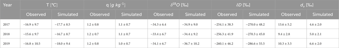
Table 1. Observed and modeled yearly mean ($\pm$ 1$\sigma$ standard deviation, derived from monthly values) of temperature $T$, specific humidity $q$, and isotope values in vapour ${\delta }^{18}O$, $\delta D$, $d_v$ at Neumayer Station III.

Next, we study daily changes of all these variables. Figure 1 compares the daily averaged outputs from the ECHAM6-wiso model and the corresponding measurements over the 3 years (from February 2017 to January 2020) of observations at Neumayer Station. The model successfully reproduces the daily observed variations, synoptic events, and seasonal cycles for (a) temperature, (b) humidity, (c) ${\delta }^{18}{O}_v$, and $\delta D_v$ (not shown) in the vapour phase. However, in the case of $d_v$ (Figure 1d), the model fails to fully capture the observed values on the daily time scale.

Figure 1

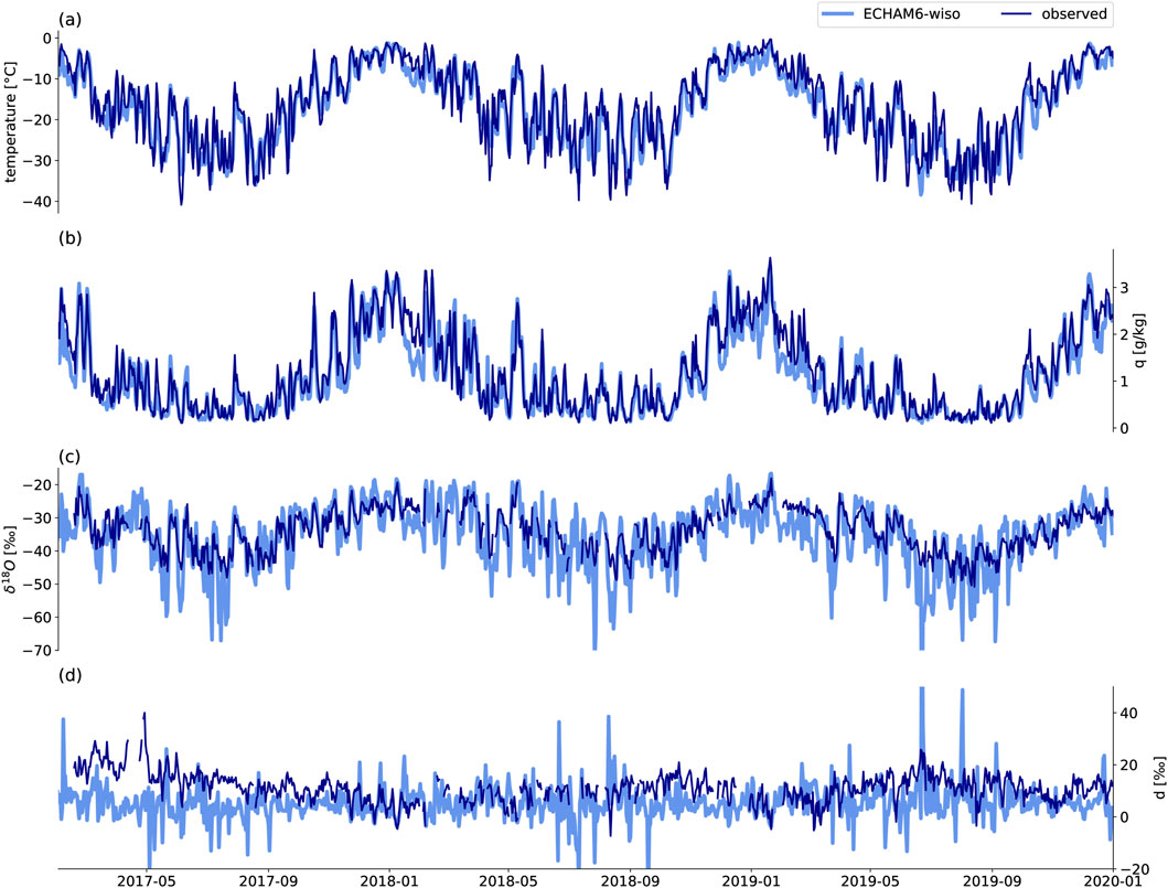
Figure 1. Observed (dark blue) vs. ECHAM6-wiso (light blue) daily variations at Neumayer Station from February 2017 to January 2020 for (a) 2-m temperature [$°$C], (b) specific humidity [ $gk{g}^{-1}$], (c) ${\delta }^{18}{O}_v$ [‰], and (e) $d_v$ [‰].

Given that the ECHAM6-wiso simulation is nudged to the ERA5 temperature data, one could expect that the model accurately reproduces the daily temperature values at Neumayer Station. The overall average temperature at Neumayer Station over the complete 3-years period is −16.4 °C for the observations, and −17.4 °C for the ECHAM6-wiso simulation. This agrees with the cold bias found for each individual year (Table 1). For mean winter (JJA) values, the simulated temperature is 0.6 °C lower than the observed one (−26.5 °C vs. −25.9 °C). Thus, the cold bias of the ECHAM6-wiso model is somewhat smaller in winter than for the annual mean. However, Figure 1a reveals that there is also an opposite warm model bias in simulated daily temperatures during extreme cold winter conditions. For days with a mean temperature less than −26.2 °C (this threshold value is the average of simulated and observed mean winter temperature values) the average observed daily temperature is −31.7 °C, while the average simulated daily temperature is −30.3 °C. Thus, for these extreme cold winter days, the ECHAM6-wiso model reveals a 1.4 °C warm bias as compared to the observations.

For ${\delta }^{18}{O}_v$, the overall mean annual observation value is −34.0‰, and the corresponding simulation value is −35.3‰. The mean winter (JJA) value of ${\delta }^{18}{O}_v$ is −40.1‰for the observations, and −43.2‰for the ECHAM6-wiso simulation. These negative isotope biases in the model results can be related to the found cold temperature bias. Interestingly, for winter days with extreme depleted isotope values this model bias is not reversed for ${\delta }^{18}{O}_v$. Considering only the days with ${\delta }^{18}{O}_v$ values less than −41.7‰(which is the average of simulated and observed winter ${\delta }^{18}{O}_v$ means), the average observed daily ${\delta }^{18}{O}_v$ value is −44.3‰, while the average simulated daily ${\delta }^{18}{O}_v$ value is −49.1‰. Thus, for these winter days with extreme low ${\delta }^{18}{O}_v$ values, which correspond well with days with extreme low temperatures (Figure 1), model ${\delta }^{18}{O}_v$ are 4.8‰lower than the observations, opposite to the found +1.4 °C warm model bias. A comparable result is found for the comparison of observed and simulated daily $\delta D_v$ values (not shown).

Next, we examine the differences between the simulation results and observations by analysing the linear relationship between the simulated and observed daily values (Figure 2a). Our analysis reveals a notable linear agreement between the observed and simulated daily temperatures, as manifested by a high correlation coefficient of 0.95 and a slope of 0.88$\pm$ 0.01 °C/°C. This slope indicates that simulated daily temperature variations during the investigated 3-years time period are slightly dampened as compared to the observations.

Figure 2

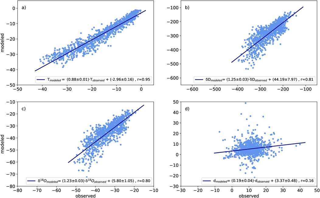
Figure 2. Observed vs. simulated daily average values for the observational period (February 2017 - January 2020) for (a) 2-meter temperature [$°$C]; (b) $\delta D_v$ [‰]; (c) ${\delta }^{18}{O}_v$ [‰]; and (d) $d_v$ [‰]. For each variable, we computed the best-fitted line, encompassing its slope, intercept, and respective uncertainties, employing the least-squares methodology for comparing observations and simulations. Subsequently, this fitted line is graphically represented as a dark blue line. We also calculated the corresponding correlation coefficient.

The simulated variables ${\delta }^{18}{O}_v$ and $\delta D_v$ align well with the observed data, with linear correlation coefficients of 0.80 and 0.81, respectively (Figures 2b,c). Despite the overall good agreement, the model amplifies daily variations of ${\delta }^{18}{O}_v$ $(\delta D_v)$ as compared to the observations, as evidenced by a slope of 1.23$\pm$ 0.03‰/‰(1.25$\pm$ 0.03‰/‰) between the observed and simulated isotope values. This tendency for amplified fluctuations can also be seen in Figure 1, where the simulated ${\delta }^{18}{O}_v$ values follow the observed ones but often exhibit larger variations on the daily time scale. Taking into consideration the known strong influence of local temperature and specific humidity on the observed fluctuations in ${\delta }^{18}{O}_v$ and $\delta D_v$ at Neumayer Station III, as already reported in Bagheri Dastgerdi et al. (2021), as well as the slightly dampened simulation of daily temperature variations by the ECHAM6-wiso model, we conclude that the influence of daily temperature variations on the daily ${\delta }^{18}{O}_v$ variations is amplified in ECHAM6-wiso as compared to the observations.

Our analysis reveals a weak correlation coefficient (r = 0.16) between the observed and simulated daily $d_v$ values (Figure 2d), which supports the found deficit of ECHAM6-wiso to correctly simulate daily variations of $d_v$ (Figure 1d). To further assess the model’s capability in capturing $d_v$ over shorter time series, we compute the correlation coefficients between observed and simulated data for a 10-day rolling interval, spanning from 5 days preceding to 5 days following the target day, for the whole 3-years observation period. This rolling correlation analysis reveals that nearly 45% of the rolling 10-day intervals have a correlation coefficient exceeding 0.5, implying that the ECHAM6-wiso model is at least partially capable of simulating $d_v$ changes over shorter periods of 10-days. An assessment of the correlation coefficient across different seasons reveals that during summer (DJF), 65% of the 10-day-intervals have a correlation coefficient above 0.5, while during winter, this value drops to 34%. This seasonal difference in the model’s ability to simulate daily $d_v$ variations may be attributed to the varying uncertainties associated with $d_v$ during different seasons. An examination of the seasonal average $d_v$ uncertainty indicates that the simulated $d_v$ has greater uncertainties during winter compared to summer. The average monthly uncertainties of simulated $d_v$ during summer and winter are 5.49‰and 9.61‰, respectively. Chapter 4 will delve into the factors contributing to the suboptimal performance of the ECHAM6-wiso model in simulating $d_v$, particularly during the winter season.

3.1.1 ${\delta }^{18}{O}_v$ vs. temperature

Next, we study the relationship between daily 2-meter temperature and ${\delta }^{18}{O}_v$ changes at Neumayer Station for both the observational data and the simulation results (Figure 3). From the observational dataset, we detect a strong correlation between the 2-meter temperature and ${\delta }^{18}{O}_v$, with a slope of 0.56$\pm$ 0.01‰/°C and a correlation coefficient of 0.87. For the simulated 2-meter temperature and ${\delta }^{18}{O}_v$ values, a steeper slope of 0.81$\pm$ 0.02‰/°C and a slightly lower correlation coefficient of 0.77 are found. Furthermore, as clearly seen in Figure 3, the simulated ${\delta }^{18}{O}_v$-temperature relation shows an increased variability as compared to the observed relationship between these two variables.

Figure 3

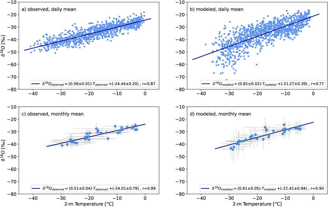
Figure 3. 2-meter air temperature [$°$C] vs. ${\delta }^{18}O$ [‰]. (a) Observed data, daily mean values; (b) simulated data, daily mean values; (c) observed data, monthly humidity-weighted mean values; (d) simulated data, monthly humidity-weighted mean values. For each plot, a best fitted line, using the least-squares approach, for 2-meter temperature vs. ${\delta }^{18}O$ is shown as a dark blue line and corresponding correlation coefficients are given.

To achieve a more comprehensive understanding between the observed and simulated temperature-${\delta }^{18}{O}_v$-relationship, we also look at humidity-weighted monthly mean ${\delta }^{18}{O}_v$ values as part of our analyses. This approach yields a slope of 0.51$\pm$ 0.04‰/°C for the relationship between 2-m temperature and ${\delta }^{18}{O}_v$ for observed monthly values, close to the slope of 0.56‰/°C calculated for the observed daily temperature and ${\delta }^{18}{O}_v$ values. For the ECHAM6-wiso simulation results we find a temperature-${\delta }^{18}{O}_v$-relationship with a slope of 0.61$\pm$ 0.05‰/°C, which is in good agreement with the observed one. To better understand the cause behind this difference in slopes between simulated daily and humidity-weighted monthly means, we additionally analyse the relationship between modeled monthly mean temperatures and the arithmetic (not humidity-weighted average) monthly mean ${\delta }^{18}{O}_v$ values. For this case we calculate a slope of 0.72$\pm$ 0.05‰/°C, closer to the slope of 0.81$\pm$ 0.02‰/°C based on daily ${\delta }^{18}{O}_v$ values. This indicates that more than half of the strong decrease in the temperature-${\delta }^{18}{O}_v$-slope for humidity-weighted monthly ${\delta }^{18}{O}_v$ values is caused by the applied humidity-weighting approach, and a lesser part by the averaging of daily to monthly ${\delta }^{18}{O}_v$ data.

In a next step, we have looked closer at the ECHAM6-wiso ${\delta }^{18}{O}_v$ bias for days characterized by relatively low humidity levels. Based on the daily data, the difference between the humidity-weighted monthly mean and arithmetic monthly mean ${\delta }^{18}{O}_v$ values is 1.17‰on average for the summer months (DJF). In contrast, this difference rises to an average of 3.82‰for the winter months (JJA). To estimate the effect of this bias on the temperature-${\delta }^{18}{O}_v$-relationship, we have calculated the (humidity-weighted) ${\delta }^{18}{O}_v$-T relationship not only for the complete dataset (shown in Figure 3), but also for the daily ${\delta }^{18}{O}_v$ and T data of the driest/wettest 20th percentile of daily vapour data. For such subset of observed dry vapour values, we retrieve a similar temperature-${\delta }^{18}{O}_v$ slope (0.65$\pm$ 0.19) as for the complete data set (0.51$\pm$ 0.04). The uncertainty of the estimated slope is higher due to the lower number of dry months available for the calculation. Similar results are found for the ECHAM6-wiso data with a slope of 0.67$\pm$ 0.40 for dry days (as compared to 0.61$\pm$ 0.05 for all days). We retrieve similar results if we analyse the 10th percentile or 25th percentile of daily vapour data instead of the 20th percentile (not shown). From these results we conclude that the found improved model-data agreement due to humidity-weighting is also valid for extremely arid days. Interestingly, our analyses yield very different, unphysical negative temperature-${\delta }^{18}{O}_v$ slopes for the wettest 20th-percentile data (not shown). At this point we do not have a full explanation for this finding but we assume that extremely wet days might be related to moist, warm air intrusions (similar to cases in the Arctic studied in Brunello et al. (2024) which might lead to a different temperature-${\delta }^{18}{O}_v$ relationsship.

3.1.2 Snow

During the observation period of 2017–2020, no snow samples were collected in parallel with the vapour measurements. Therefore, for a comparative analysis of observed and simulated values of the isotope ratio of snow $({\delta }^{18}{O}_{\mathit{snow}})$ falling at Neumayer Station, we analyze snowfall samples from an earlier period. Between the years 1981 and 2000, fresh snow samples were sampled at the Neumayer Station following significant snowfall events (Schlosser, 1999). These snowfall occurrences are associated with pronounced wind activity. Consequently, the acquired snow samples represent a mixture of freshly precipitated snow and airborne or ‘blowing’ snow (Schlosser, 1999). For the model-data comparison, we use the ECHAM6-wiso monthly values of ${\delta }^{18}{O}_{\mathit{snow}}$ and 2-meter temperature covering the same 2 decades (1981–2000) as the observation values.

The average ${\delta }^{18}{O}_{\mathit{snow}}$ value calculated from all snow samples collected during the period 1981–2000 is −20.5‰. The mean ECHAM6-wiso simulation value of ${\delta }^{18}{O}_{\mathit{snow}}$ for the same period is −22.10‰. From the observational data, we calculate a 2-meter temperature-${\delta }^{18}{O}_{\mathit{snow}}$-relation with a slope of 0.59$\pm$ 0.05 $\text{‰}°C^{-1}$ $(r=0.71)$ for the aforementioned period (Figure 4). The corresponding slope based on simulated 2-meter temperature and ${\delta }^{18}{O}_{\mathit{snow}}$ values is only 0.44$\pm$ 0.02 $\text{‰}°C^{-1}$ $(r=0.82)$. This disagreement of observed and simulated 2-meter temperature-${\delta }^{18}O$-slopes for monthly snow samples is in clear contrast to the found agreement of observed and simulated 2-meter temperature-${\delta }^{18}O$-slopes for monthly humidity-weighted vapour values.

Figure 4

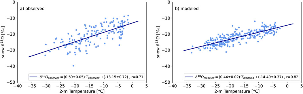
Figure 4. 2-meter air temperature [$°$C] vs. ${\delta }^{18}{O}_{\mathit{snow}}$ [‰] for years 1980–2000. (a) Observed data, monthly mean values; (b) simulated data, monthly mean values. For each sub-figure, a best fitted line, using the least-squares approach, for 2-meter temperature vs. ${\delta }^{18}{O}_{\mathit{snow}}$ is plotted as a dark blue line and corresponding correlation coefficients are calculated.

3.1.3 Transport pathway and water source origins

Focusing on the full observational period 2017–2019, we examine the main moisture uptakes for water vapour transported to Neumayer Station, as simulated by the FLEXPART model. Figure 5 illustrates the seasonal means of moisture uptake for the last 10 days of air parcel trajectories ending at Neumayer Station. Comparing the general patterns of FLEXPART results based on either the ECHAM6-wiso or the ERA5 forcing data, both simulations indicate similar origins for the water vapour transported to Neumayer Station. In spring, the primary moisture uptakes are from ocean areas northwest of the station, situated at high to mid-latitudes. During summer and autumn, the primary water uptake mainly occurs in coastal regions close to Neumayer Station, but minor additional moisture uptakes occur from the Southern Ocean at mid-latitudes. In winter, the moisture flow to Neumayer Station substantially decreases compared to other seasons; however, source regions still span a wide area of the Southern Ocean, with some contributions even from the Pacific. Bagheri Dastgerdi et al. (2021) already showed that the season-dependent moisture origin variations for Neumayer Station are influenced by several factors such as sea ice extent, 6-month semi-annual atmospheric oscillation, and temperature changes in the source regions.

Figure 5

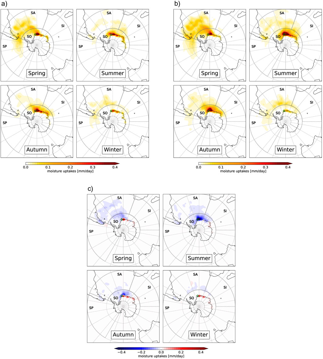
Figure 5. Simulated mean moisture uptake occurring within the boundary layer $[mmda{y}^{-1}]$ in the pathway to Neumayer Station during last 10 days modelled by FLEXPART for spring (SON), summer (DJF), autumn (MAM), and winter (JJA), considering the mean values of the years of 2017, 2018, and 2019 using (a) ECHAM6 output; (b) ECMWF, ERA5 data set. (c) shows the anomaly plot (ECHAM6-wiso based simulations minus ERA5 based simulations). The dotted lines mark the borders of the four defined source regions Southern Ocean (SO), Southern Atlantic (SA), Southern Pacific (SP), and Southern Indian Ocean (SI).

While FLEXPART simulations based on ECHAM6-wiso (Figure 5a) successfully reproduce the seasonal patterns retrieved when using FLEXPART in combination with the ERA5 dataset (Figure 5b), the anomaly plot in Figure 5c reveals some differences in the amount of moisture uptake between the two approaches. Specifically, in spring, autumn, and winter, the FLEXPART simulation based on ECHAM6-wiso data exhibits more water evaporating from coastal land areas tranported to Neumayer Station as compared to the FLEXPART simulation based on the ERA5 dataset. Conversely, FLEXPART simulation results based on ECHAM6-wiso show less water evaporating from the other ocean source regions transported to Neumayer Station as compared to the FLEXPART simulation forced by ERA5 data.

For a more quantitative analyses of the FLEXPART results, we have defined four major evaporation regions of water vapour transported to Neumayer III Station: the nearby coastal Southern Ocean (80S-60S, 68W-120E), the Southern Atlantic (60S-30S, 68W-20E), Southern Pacific (80S-30S, 150W–68W) and Southern Indian Ocean (60S-30S, 20E-90E). For each of these regions we have calculated for all four seasons the total amount of moisture uptaken from the surface to the atmospheric boundary layer (Table 2). Our analyses reveal that more than 98% of all vapour transported to Neumayer Station III stems from these four regions with a clear dominance of the Southern Ocean region in all seasons. Our FLEXPART analyses also show that the ECHAM6-wiso simulation captures the percentage of distributions in agreement with results obtained from ERA5, but the ECHAM6-wiso model underestimates the absolute amount of moisture uptake by approximately 10%–50% as compared to the ERA5 results.

Table 2

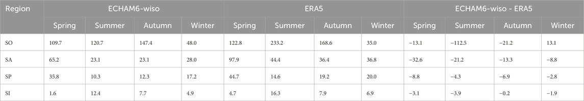
Table 2. Seasonal mean moisture uptake fluxes integrated over key vapour source regions as derived from the FLEXPART model based on either ERA5 or ECHAM6-wiso forcing. Austral seasons are different by calendar months (spring SON, summer DJF, autumn MAM, winter JJA). Key vapour source regions are the Southern Ocean SO, Southern Atlantic SA, Southern Pacific SP, and Southern Indian Ocean SI (see details in the text for the geopgrahic extent of these regions). The differences between the ERA5 and ECHAM6-wiso fluxes are shown on the right hand of the table. All moisture uptake values are given mm/day.

4 Discussion

In the past years, the ECHAM-wiso model performance related to isotope values has been thoroughly tested for its sensitivity against some key parameters, e.g., model resolution (Werner et al., 2011; Cauquoin and Werner, 2021), fractionation during supersaturation (Werner et al., 2011), evaporation from open ocean and sublimation over sea ice (Bonne et al., 2019; Gao et al., 2025) and source region dependencies (Gao et al., 2024). It has been shown in several recent studies that the ECHAM6-wiso model shows a very good performance when compared to ${\delta }^{18}O$ measurements in Antarctic snow and vapour, in general (e.g., Servettaz et al., 2020; Leroy-Dos Santos et al., 2023; Dreossi et al., 2024; Ollivier et al., 2025). From these earlier studies, we conclude that the model bias observed at Neumayer Station III is most likely caused by the station’s location near the coast, and we analyse this bias in detail in the following.

4.1 Temperature and humidity

Our analyses reveal clear deviations between observed and ECHAM6-wiso modeled temperature and humidity values (Chapter 3.1, Table 1), leading to a cold and dry model bias. To better understand these deviations we look at potential differences, how the 2-m temperature and near-surface humidity values are derived in the observational data set and in ECHAM6-wiso.

At Neumayer Station, continuous temperature measurements at a 2-meter are taken in the close vicinity of the station (Chapter 2.2). On the contrary, simulated ECHAM6-wiso temperatures are primarily controlled by the 3D temperature fields of the ERA5 data set, which are used for the 6-hourly nudging of the ECHAM6 simulation (Chapter 2.3). These ECHAM6 nudging adjustments are made to align with ERA5 temperature data on model level values, but not directly with the ERA5 2-meter temperature data. Consequently, the 2-meter temperature data for both ERA5 and ECHAM6 are derived independently, by further calculation.

In Figure 6, we compare the daily and monthly mean 2-meter temperatures as recorded in observations from Neumayer Station, ECHAM6 simulations, and the ERA5 reanalysis dataset. Both the ERA5 and ECHAM6 dataset are highly correlated with the observed 2-meter temperature at the station (correlation coefficient of 0.98 and 0.96, respectively). However, the ERA5 dataset shows a positive warm bias, especially for the winter season, while the ECHAM6 data shows a slight negative bias in all months. On average, the ERA5 2-meter temperature (−14.74 °C) is 1.69 °C higher than the observed temperature (−16.43 °C), and the ECHAM6 mean 2-meter temperature (−17.46 °C) is 1.03 °C lower than observed. On a day-to-day basis, ERA5 temperatures are higher than the directly measured temperatures at Neumayer Station for 82% of all days during our 3-years observational period, while simulated ECHAM6 temperatures are lower in 67% of all days.

Figure 6

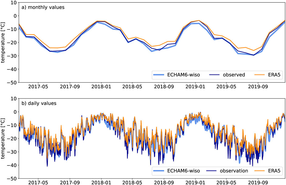
Figure 6. 2-meter temperature [°C] derived from direct station measurements, ECHAM6-wiso simulation results, and ECMWF-ERA5 reanalysis data at Neumayer Station from February 2017 to January 2020; (a) monthly mean values; (b) daily mean values.

The deviation between observed 2m-temperatures and ERA5 values can be explained by the fact that ERA5 computes these near-surface air temperatures through a process of interpolation between the surface temperature and the temperature at the lowest model atmospheric level. This interpolation might be erroneous under certain meteorological and coastal surface conditions, e.g., varying sea ice cover in the vicinity of Neumayer Station. Furthermore, the ERA5 reanalysis data represent averaged values over the spatial extent of a grid cell, in contrast to the location-specific point measurements conducted at Neumayer Station (Xie et al., 2014; Zhang et al., 2018). At the geographic coordinates of the Neumayer Station, situated at a latitude of 70°S, the east-west span of an ERA5 grid cell is approximately 9.52 km. This difference might also partly explain the deviations between the ERA5 data and the direct temperature measurements at the station.

For the simulation used in this study, the ECHAM6 model is nudged towards the three-dimensional fields of temperature, vorticity, divergence, and surface pressure fields of the ERA5 dataset. Therefore, it was expected that the 2m-temperature values of the ECHAM6-wiso simulation are highly correlated with the 2-meter temperatures of the ERA5 dataset. However, clear discrepancies between the ERA5 and ECHAM6-wiso temperature values exist (Figure 6). These differences might be caused by the different vertical and horizontal resolution of the two datasets: The ERA5 data includes temperature values across 137 atmospheric model levels and a horizontal grid resolution of approximately 0.25° by 0.25°, whereas the ECHAM6-wiso data includes only 95 vertical model levels, and also a coarser horizontal grid resolution of approximately 0.9° by 0.9°.

In contrast to atmospheric temperatures, the ECHAM6-wiso model is not nudged to ERA5 humidity data in our simulation. Thus, simulated specific humidity data at the 2-meter level is an ERA5-independent ECHAM6-wiso model variable, which we compare with the observed specific humidity at Neumayer Station. To ensure a comprehensive analysis, we also include the 2-meter ERA5 specific humidity, which is calculated from the 2-meter surface dew point temperature and surface pressure. As shown in Figure 7, both ERA5 and ECHAM6 values closely match the directly measured specific humidity at Neumayer Station, with high correlation coefficients (0.98 and 0.96, respectively). The ERA5 data shows a slightly higher agreement with and smaller offset from the observed specific humidity as compared to the ECHAM6-wiso values. The mean specific humidity at Neumayer Station over the complete observational period was 1.18 g/kg for the direct measurements, 1.19 g/kg for ERA5, and 1.10 g/kg for ECHAM6-wiso. ECHAM6-wiso underestimates the specific humidity in 91% of all months, while the ERA5 reanalyses data underestimates the measured specific humidity at Neumayer Station only during the summer months, but overestimates it in most other months. The reason for this ECHAM6-wiso model mismatch remains unclear. It may be due to an insufficiently resolved vertical humidity gradient in the lowest ECHAM model layers, or to biases in the prescribed meteorological and coastal surface conditions for the ECHAM6-wiso simulation.

Figure 7

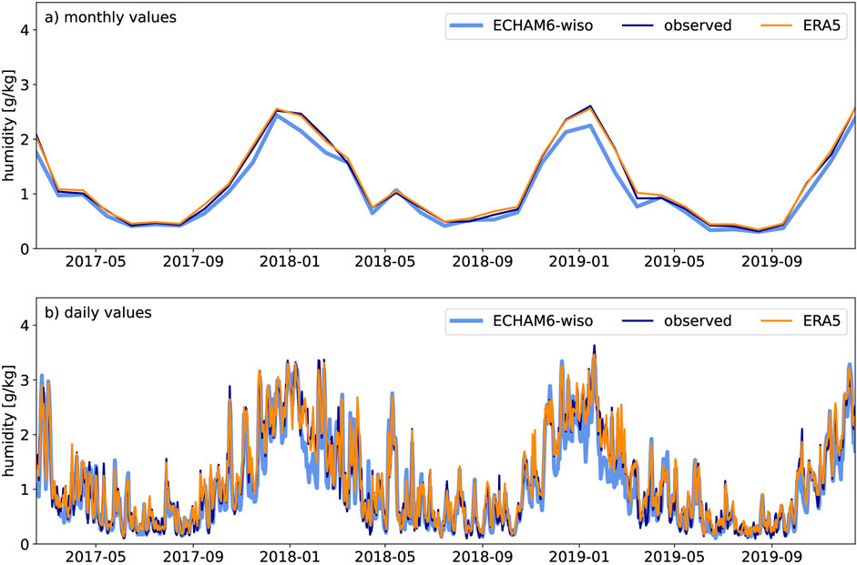
Figure 7. 2-meter specific humidity [g/kg] derived from direct station measurements, ECHAM6-wiso simulation results, and ECMWF-ERA5 reanalysis data at Neumayer Station from February 2017 to January 2020; (a) monthly mean values; (b) daily mean values.

4.2 ${\delta }^{18}O$ in water vapour

Bagheri Dastgerdi et al. (2021) demonstrated that local temperature is the primary factor influencing variations in ${\delta }^{18}{O}_v$ at Neumayer Station. Although there is a strong correlation (r = 0.80) between simulated and observed daily ${\delta }^{18}{O}_v$ values, simulated day-to-day ${\delta }^{18}{O}_v$ variability is substantially larger in ECHAM6-wiso as compared to the observations. As the large-scale circulation of our ECHAM6-wiso simulation is nudged towards ERA5 data every 6 h, these deviations cannot be explained by an erroneous higher model variability of vapor transport to the Neumayer Station III. The relatively large grid cell of the ECHAM6-wiso model, which covers the location of Neumayer Station III and extends over approximately 1 ° × 1 °, should smooth rather than distort the modelled day-to-day ${\delta }^{18}{O}_v$ variability. One process which might lead to a higher modelled ${\delta }^{18}{O}_v$ variability as compared to observations is a potential post-depositional exchange of water isotopes between snow and the near-surface vapor. Recent studies (e.g., Steen-Larsen et al., 2014; Casado et al., 2016; Casado et al., 2018; Dietrich et al., 2023) suggest that such exchange processes are non-negligible. These exchange processes can occur on a daily time scale (Ritter et al., 2016) and could dampen the observed ${\delta }^{18}{O}_v$ signal at Neumayer Station III. As these processes are not yet included in the ECHAM6-wiso model, such post-depositional vapor-snow ${\delta }^{18}{O}_v$ exchange could explain the deviations in observed and modelled ${\delta }^{18}{O}_v$ variability.

Differences between simulated and observed ${\delta }^{18}{O}_v$ values are found particularly under extreme cold conditions. These differences can be seen in Figure 1, with extreme low simulated ${\delta }^{18}{O}_v$ values during numerous cold days. A detailed analysis of the coldest 5% of days of our 3-years observation period yields a clear difference between observed and simulated ${\delta }^{18}{O}_v$ values. The average observed daily ${\delta }^{18}{O}_v$ value is −43.76‰, whereas the simulated average is −49.60‰. Notably, no observed value is below −51‰, yet the simulation contains 72 daily ${\delta }^{18}{O}_v$ values below this threshold, including 15 days with ${\delta }^{18}{O}_v$ values below −60‰, indicating a clear ${\delta }^{18}{O}_v$ bias of ECHAM6-wiso under extreme conditions. These findings are in line with similar ${\delta }^{18}{O}_v$ deficits reported for ECHAM6-wiso in the Arctic winter (Brunello et al., 2023) and might indicate an insufficient representation of boundary layer moisture transport (Sigmund et al., 2023).

We move in our analysis from a daily to a monthly view in order to analyse the dynamics of ${\delta }^{18}{O}_v$ changes on a coarser time scale. The monthly average values of both the simulated and observed ${\delta }^{18}{O}_v$ values are shown in Figure 8. Standard deviations of the simulated and observed monthly mean ${\delta }^{18}{O}_v$ values are calculated from the time series of daily values. The simulation results display a more pronounced day-to-day variation in ${\delta }^{18}{O}_v$ as compared to the observations, especially in the austral winter season, as visualized in Figure 8a.

Figure 8

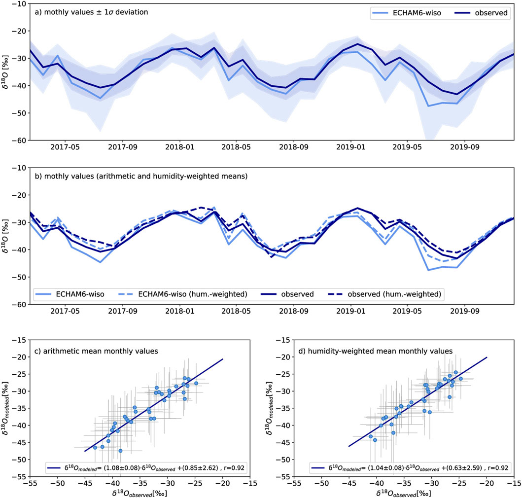
Figure 8. Monthly mean simulated ${\delta }^{18}{O}_v$ vs. observed ${\delta }^{18}{O}_v$ values at Neumayer Station from February 2017 to January 2020; (a) time series of monthly mean values $\pm 1$ standard deviation. (b) Time series of arithmetic (solid lines) and humidity-weighted (dashed lines) monthly mean values. (c) Scatter plot of observed vs. simulated arithmetic mean monthly ${\delta }^{18}{O}_v$ values with a best-fitted line, using the least-squares approach and calculated correlation coefficient; (d): as (c), but for humidity-weighted mean values.

A comparison of normal arithmetic monthly averages and humidity-weighted averages show strong agreement between simulated and observed monthly ${\delta }^{18}{O}_v$ values, with correlation coefficients over 0.90 for both methods (Figures 8b,c). The linear relationship between the observed and simulated humidity-weighted monthly averages has a slope of 1.04$\pm$ 0.08, suggesting an adequate model performance in capturing monthly fluctuations. The slope for normal monthly averages is 1.08$\pm$ 0.08, which is slightly higher than the one calculated for the humidity-weighted values. The same is true for the y-intercept, where the intercept for humidity-weighted averages is 0.63$\pm$ 2.59, which is again slightly lower than the intercept value for normal monthly averages (0.85$\pm$ 2.62).

Despite some improved agreement between the observations and the ECHAM6-wiso results for monthly ${\delta }^{18}{O}_v$ data, as compared to the daily data, the model results still reveal the strongest bias for extremely cold and dry conditions. Considering the influence of the specific humidity on the simulated isotope values by looking at humidity-weighted ${\delta }^{18}{O}_v$ values, partially resolves this bias. Regarding the temperature-${\delta }^{18}{O}_v$ relation, the observed agreement of the modeled and observed slope (0.51 compared to 0.61) and intercept (−24.01 compared to −22.41) emphasises the ability of the ECHAM6-wiso model to accurately represent the temperature-${\delta }^{18}{O}_v$ relationship at monthly time scale. However, it’s important to acknowledge the model’s constraints, particularly under conditions of extremely dry and cold environments.

4.3 ${\delta }^{18}O$ in snow

We used the analysis of 20 years of temperature and ${\delta }^{18}{O}_v$ data (1980–2000) collected at Neumayer Station (Schlosser, 1999). The observed slope is 0.59‰/°C, whereas the slope derived from simulated values is 0.44‰/°C. To better understand these results, we investigated the relationship between simulated monthly mean ${\delta }^{18}{O}_v$ and 2-meter temperature. We find here a slope of 0.61‰/°C, which is in better agreement with the observed ${\delta }^{18}{O}_v$-temperature slope (0.51‰/°C for the years 2017–2020), but which also agrees well with the observed ${\delta }^{18}{O}_{\mathit{snow}}$-temperature slope of 0.59‰/°C (for the period 1980–2020).

One possible explanation for these differences is that the model does not take into account the isotopic exchanges between the surface snow and the water vapour above it. Recent studies reported such isotopic exchanges, especially for regions like Greenland (Steen-Larsen et al., 2014; Madsen et al., 2019; Dietrich et al., 2023) and Antarctica (Casado et al., 2016; Casado et al., 2018). Specifically, Steen-Larsen et al. (2014) found in a field study on Greenland that the isotope ratio of surface snow between snowfall events tends to align closely with that of water vapour above the snow surface. Steen-Larsen et al. (2014) proposed that changes in the surface snow isotopic composition might thus be linked to fluctuations in related water vapour isotopic concentrations. Drifting snow also undergoes further isotopic fractionation processes which might alter the isotopic composition of near-surface water vapour (Wahl et al., 2024). Such post-depositional vapour-snow isotope exchange is currently not implemented in the ECHAM6-wiso model, but the process could be crucial for an improved simulation of the ${\delta }^{18}{O}_{\mathit{snow}}$-temperature relationship at Neumayer Station, as well as for other locations in both Antarctica and Greenland.

Our analyses might also be hampered by the different time period of the taken snow samples (1981–2000) and the measured vapour values (2017–2019) as environmental conditions might have changed between the two periods. Temperatures at the precipitation site and sea ice coverage around Antarctica are among the key controlling factors of the isotope signals both in snow and vapour at Neumayer Station. Therefore we have analysed 2 m air temperature measurements at Neumayer, which are available since March 1982 (Schmithüsen, 2023), and total Antarctic sea ice concentration, which are available since January 1973 (Spreen et al., 2008; Melsheimer and Spreen, 2019). For the two periods of interest, no substantial changes were identified in either 2 m temperatures (1981–200: −15.77 $\pm$ 1.32 °C; 2017–2019: −16.03 $\pm$ 0.61 °C) or Antarctic sea ice concentration (1981–200: 11.51 $\pm$ 0.19 Mio.$k{m}^2$; 2017–2019: 10.83 $\pm$ 0.10 Mio.$k{m}^2$). We conclude that the time lag between the analysed snow samples and vapour measurements can be neglected for our analyses results.

4.4 Model deficits in simulating $d_v$

The uncertainty of the measured $d_v$ values at Neumayer Station is very high for a large period due to the low humidity at Neumayer Station (Section 2.1) and the limited precision of the Picarro instrument for such low humidity values. This deficit of our measurements was already discussed in more detail by Bagheri Dastgerdi et al. (2021), who showed that the monthly average uncertainty for $d_v$ in austral winter at Neumayer Station is up to 4.5‰. Bagheri Dastgerdi et al. (2021) reported a negative correlation between specific humidity and $d_v$ during spring (r = −0.50), summer (r = −0.71), and autumn (r = −0.24), whereas a slight positive correlation was observed in winter (r = 0.13). In our study the observed correlation coefficient between specific humidity and $d_v$ across all months is −0.43, in agreement with the previous findings. However, the ECHAM6-wiso simulation results show a correlation of only −0.17 for $d_v$ and specific humidity, indicating that the ECHAM6-wiso model fails to capture the relationship between $d_v$ and specific humidity in a correct manner.

In a previous study, (Steen-Larsen et al., 2017), have already compared model results of different isotope-capable AGCMs for the simulation of $d_v$ in the marine boundary layer. They were able to show that the $d_v$ signal depends primarily on the model parameterisations for kinetic fractionation effects during the evaporation of water from the ocean surface and less on the simulation of the absolute humidity values themselves. Assuming that the $d_v$ signal generated by evaporation processes above the ocean surface is transported to Neumayer Station without major changes, then this model-dependent parameterisation of kinetic fractionation processes will also play an important role for the model-data comparison of $d_v$ at Neumayer Station. In addition, it remains open if the suggested post-depositional isotopic exchange between vapour and surface snow, which is not included in the ECHAM6-wiso model yet, might also change the $d_v$ signal.

4.5 Dependency of ECHAM6-wiso model results on prescribed boundary conditions

In this study, the ECHAM6-wiso model is used for the various model-data comparisons with the isotope measuremets performed at Neumayer Station. At the beginning of our study, initial ECHAM6-wiso simulation results did not agree with the isotope measurements at Neumayer Station well. The model exhibited a tendency to clearly overestimate the absolute ${\delta }^{18}{O}_v$ values by several permill and also to underestimate the seasonal amplitude of ${\delta }^{18}{O}_v$ changes (Figure 9). This result was surprising given the fact that older simulations results from the previous model release ECHAM5-wiso agreed well in general with observations from Neumayer Station. It was expected that the ECHAM6-wiso model would perform at least as well as, if not better than its predecessor. To understand this unexpected ECHAM6-wiso model deficit, a comparison from an older ECHAM5-wiso simulation, which was nudged to the older ERA-Interim dataset (available up to 2018), with the new ECHAM6-wiso/ERA5 simulation was performed. The ${\delta }^{18}{O}_v$ values simulated by ECHAM5-wiso were cleary in much better agreement with the ${\delta }^{18}{O}_v$ measurements at Neumayer Station, as compared to the ECHAM6-wiso results (Figure 9).

Figure 9

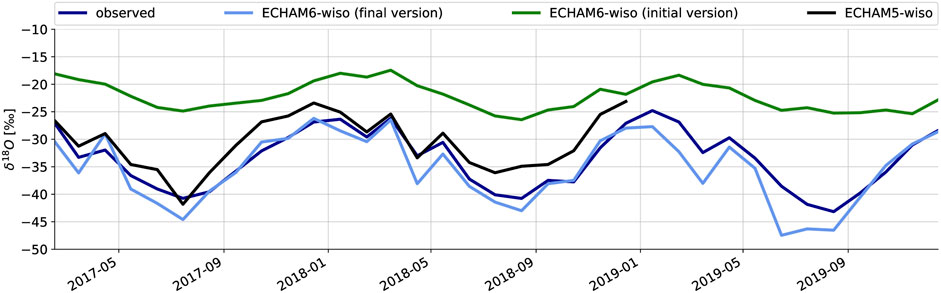
Figure 9. Monthly mean ${\delta }^{18}{O}_v$ at Neumayer Station III from February 2017 to January 2020 as measured by the Picarro analyzer (dark blue line), simulated by ECHAM6-wiso, final version (light blue line), ECHAM6-wiso, initial version (green line), and ECHAM5-wiso, until 12/2018 (black line).

Taking into account that the relevant physical processes and mechanisms are implemented in the ECHAM5-wiso and ECHAM6-wiso model in a very similar manner (Cauquoin and Werner, 2021), we examined both the used boundary conditions and forcing fields of our ECHAM6-wiso simulation, as both differ from the previous ECHAM5-wiso simulation.

For the different forcing fields used for nudging (ECHAM5-wiso: ERA-interim; ECHAM6-wiso: ERA5), no notable difference between the two data sets was found. For both the 2m-temperature and the surface pressure, the ERA5 values are in a bit better agreement with the observational data at Neumayer Station as compared to the older ERA-interim data. This finding is in agreement with a more global comparison of ERA5 vs. ERA-interim nudging fields used for the ECHAM-wiso model (Cauquoin and Werner, 2021). The result indicated that the discrepancies in the simulated ${\delta }^{18}{O}_v$ signal between ECHAM5-wiso and ECHAM6-wiso can not be attributed to the prescribed ERA5 forcing fields.

Further investigation into the different performances of ECHAM5-wiso and ECHAM6-wiso simulations included the examination of different prescribed boundary conditions, namely, the land-sea mask, the glacier mask, and variations in prescribed sea ice fraction. At the same time, simulated key variables directly influenced by these boundary conditions, namely, evaporation rates, near-surface vapour, and ${\delta }^{18}{O}_v$, were closely examined.

We found a noticeable difference between the simulated evaporation flux (Figures 10f,g,i,j) and specific humidity values (not shown) in the vicinity of the Neumayer Station for the ECHAM5-wiso and ECHAM6-wiso simulation results. We could show that these differences are not caused by a change of open ocean and sea ice covered regions, as the prescribed sea ice fraction in both simulations was comparable (Figures 10a–d).

Figure 10

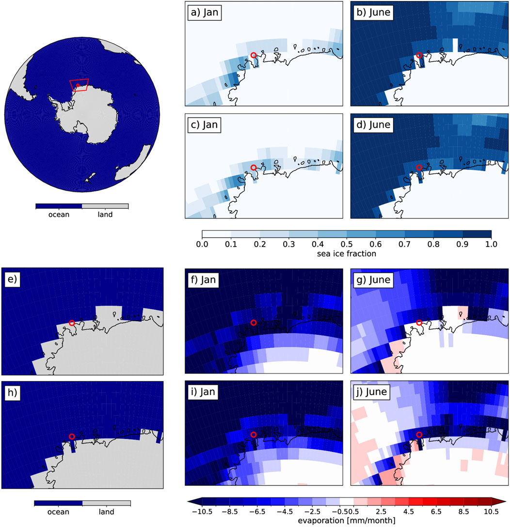
Figure 10. (1) Model results of ECHAM5-wiso vs. ECHAM6-wiso initial version. Prescribed sea ice fraction in ECHAM5-wiso for (a) January 2017, (b) June 2017, and in ECHAM6-wiso for (c) January 2017, (d) June 2017. Evaporation fluxes simulated by ECHAM5-wiso for (f) January 2017, (g) June 2017, and by ECHAM6-wiso for (i) January 2017, (j) June 2017. Prescribed land-sea-mask of (e) ECHAM5-wiso and (h) ECHAM6-wiso.

However, a clear difference impacting the simulation of near-surface water vapour around Neumayer Station in ECHAM5-wiso and ECHAM6-wiso was found to be the prescribed land-sea mask. The ECHAM6-wiso land-sea mask classified the grid box which encompasses the location of Neumayer Station as an ocean region (Figure 10h), while it was classified as a land region in ECHAM5-wiso (Figure 10e). In reality, the station is located on the 200-meter thick Ekström Ice Shelf, which is neither a “typical” ocean or land point. Adjusting the land-sea mask in ECHAM6-wiso, by reclassifying the grid cell enclosing Neumayer Station and a few grid cells to the east affected by predominant easterly winds as land grid points instead of ocean grid points, resulted in an ECHAM6-wiso simulation of ${\delta }^{18}{O}_v$ nuch more consistent with the observations and the former ECHAM5-wiso results (Figure 9). In Figure 11 the revised land-sea mask tailored for improved simulations at Neumayer Station, alongside the resulting changes in the evaporation flux for January and June 2017 are shown. This improved land-sea mask has been used for the ECHAM6-wiso simulation results presented and discussed in this study.

Figure 11

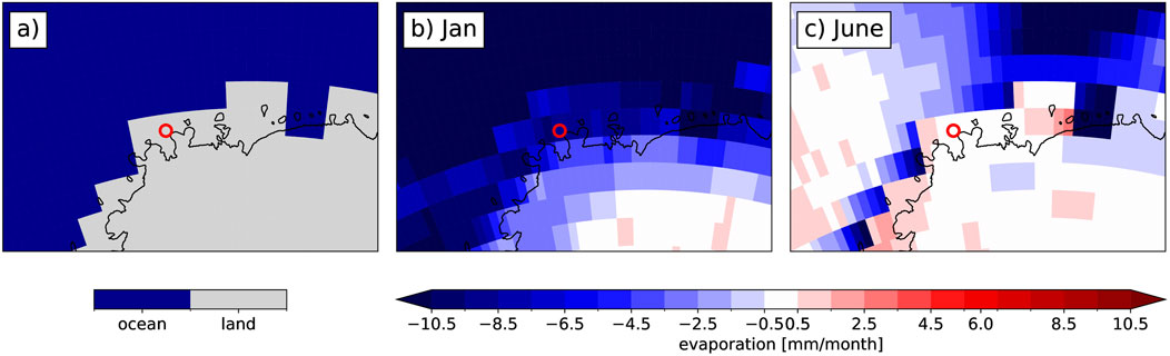
Figure 11. ECHAM6-wiso, final model version: (a) modified prescribed land sea mask, (b) simulated evaporation flux in January 2017, (c) as (b) but for June 2017.

5 Summary

This study evaluated the performance of the isotope-enabled AGCM ECHAM6-wiso against new in-situ observations of the isotopic composition of water vapour measured at Neumayer Station III, Antarctica, covering the 3-years period February 2017- February 2020.

ECHAM6-wiso successfully simulates temperature, specific humidity, and isotopic variations in water vapour (${\delta }^{18}{O}_v$, and $\delta D_v$) at daily, seasonal, and annual time scales. While the modeled annual and seasonal temperature values tend to be lower than the observed ones, the model results reveal a positive warm bias for extremely cold conditions. Simulated daily variations of ${\delta }^{18}{O}_v$ and $\delta D_v$ show a reduced sensitivity with respect to temperature changes as compared to the observations. On the monthly time scale, a better agreement between the simulated absolute isotope values in vapour and the corresponding observations can be achieved by considering humidity-weighted monthly means instead of arithmetic mean values. Such humidity-weighting also leads to a better agreement between the simulated and observed ${\delta }^{18}{O}_v$-temperature relationship. Simulated key water vapour source areas and flow paths for humidity transported from different oceanic regions to the Neumayer Station location are also in agreement with observational-based findings.

Our study also highlights some shortcomings of the analysed ECHAM6-wiso simulation, namely, in simulating water vapour d-excess variations at Neumayer Station and in simulating the observed ${\delta }^{18}O$-temperature relationship in snow in the vicinity of the station for the period 1980–2000. Post-depositional vapour-snow isotope exchange processes, which have not been implemented in the ECHAM6-wiso model yet, are identified as one potential cause for this model-data mismatch.

Overall, the results of this study strengthen our confidence in the investigation of stable water isotopes, e.g., those recorded in Antarctic ice cores, using the ECHAM6-wiso model. However, they also show that there is still room for improvement in the interpretation of ice core data using isotope-enabled climate models such as ECHAM6-wiso. If exchange processes between water vapour and snow after deposition significantly influence the isotope signal in certain ice cores, these should definitely be taken into account for a robust estimation of paleotemperatures from isotope data. Our study indicates that model refinements should include an improved simulation of vapour transport processes in the boundary layer, an explicit simulation of snow drift, and the addition of multi-layer surface snow and firn models, including isotope fractionation processes between water vapour and ice crystals in these near-surface layers. Such new model components could then lead to further advances in the interpretation of ice core data using isotope models such as ECHAM6-wiso in the future.

Data availability statement

The raw data supporting the conclusions of this article are available on the Zenodo database: https://doi.org/10.5281/zenodo.17581501, and upon request by the authors of this study, without undue reservation.

Author contributions

MW: Conceptualization, Data curation, Formal Analysis, Funding acquisition, Methodology, Resources, Supervision, Validation, Visualization, Writing – review and editing. SB: Conceptualization, Data curation, Formal Analysis, Investigation, Methodology, Visualization, Writing – original draft, Writing – review and editing. AC: Methodology, Resources, Writing – review and editing.

Funding

The author(s) declare that financial support was received for the research and/or publication of this article. This research was funded by the Helmholtz Climate Initiative REKLIM (Regional Climate Change), a joint research initiative of the Helmholtz Association of German Research Centres (HGF).

Conflict of interest

The authors declare that the research was conducted in the absence of any commercial or financial relationships that could be construed as a potential conflict of interest.

Publisher’s note

All claims expressed in this article are solely those of the authors and do not necessarily represent those of their affiliated organizations, or those of the publisher, the editors and the reviewers. Any product that may be evaluated in this article, or claim that may be made by its manufacturer, is not guaranteed or endorsed by the publisher.

References

Bagheri Dastgerdi, S., Behrens, M., Bonne, J.-L., Hörhold, M., Lohmann, G., Schlosser, E., et al. (2021). Continuous monitoring of surface water vapour isotopic compositions at neumayer station iii, east Antarctica. Cryosphere 15, 4745–4767. doi:10.5194/tc-15-4745-2021

CrossRef Full Text | Google Scholar

Barkan, E., and Luz, B. (2007). Diffusivity fractionations of Ho/Ho and Ho/Ho in air and their implications for isotope hydrology. Rapid Commun. Mass Spectrom. 21, 2999–3005. doi:10.1002/rcm.3180

PubMed Abstract | CrossRef Full Text | Google Scholar

Bolot, M., Legras, B., and Moyer, E. J. (2013). Modelling and interpreting the isotopic composition of water vapour in convective updrafts. Atmos. Chem. Phys. 13, 7903–7935. doi:10.5194/acp-13-7903-2013

CrossRef Full Text | Google Scholar

Bonne, J.-L., Behrens, M., Meyer, H., Kipfstuhl, S., Rabe, B., Schönicke, L., et al. (2019). Resolving the controls of water vapour isotopes in the Atlantic sector. Nat. Commun. 10, 1632. doi:10.1038/s41467-019-09242-6

PubMed Abstract | CrossRef Full Text | Google Scholar

Brioude, J., Arnold, D., Stohl, A., Cassiani, M., Morton, D., Seibert, P., et al. (2013). The lagrangian particle dispersion model flexpart-wrf version 3.1. Geosci. Model Dev. 6, 1889–1904. doi:10.5194/gmd-6-1889-2013

CrossRef Full Text | Google Scholar

Brunello, C. F., Meyer, H., Mellat, M., Casado, M., Bucci, S., Dütsch, M., et al. (2023). Contrasting seasonal isotopic signatures of near-surface atmospheric water vapor in the central arctic during the mosaic campaign. J. Geophys. Res. Atmos. 128, e2022JD038400. doi:10.1029/2022jd038400

CrossRef Full Text | Google Scholar

Brunello, C., Gebhardt, F., Rinke, A., Dütsch, M., Bucci, S., Meyer, H., et al. (2024). Moisture transformation in warm air intrusions into the arctic: process attribution with stable water isotopes. Geophys. Res. Lett. 51, e2024GL111013. doi:10.1029/2024gl111013

CrossRef Full Text | Google Scholar

Buizert, C., Fudge, T. J., Roberts, W. H. G., Steig, E. J., Sherriff-Tadano, S., Ritz, C., et al. (2021). Antarctic surface temperature and elevation during the last glacial maximum. Science 372, 1097–1101. doi:10.1126/science.abd2897

PubMed Abstract | CrossRef Full Text | Google Scholar

Butzin, M., Werner, M., Masson-Delmotte, V., Risi, C., Frankenberg, C., Gribanov, K., et al. (2014). Variations of oxygen-18 in West Siberian precipitation during the last 50 years. Atmos. Chem. Phys. 14, 5853–5869. doi:10.5194/acp-14-5853-2014

CrossRef Full Text | Google Scholar

Casado, M., Landais, A., Masson-Delmotte, V., Genthon, C., Kerstel, E., Kassi, S., et al. (2016). Continuous measurements of isotopic composition of water vapour on the east antarctic Plateau. Atmos. Chem. Phys. 16, 8521–8538. doi:10.5194/acp-16-8521-2016

CrossRef Full Text | Google Scholar

Casado, M., Landais, A., Picard, G., Münch, T., Laepple, T., Stenni, B., et al. (2018). Archival processes of the water stable isotope signal in east antarctic ice cores. Cryosphere 12, 1745–1766. doi:10.5194/tc-12-1745-2018

CrossRef Full Text | Google Scholar

Casado, M., Hébert, R., Faranda, D., and Landais, A. (2023). The quandary of detecting the signature of climate change in Antarctica. Nat. Clim. Change 13, 1082–1088. doi:10.1038/s41558-023-01791-5

CrossRef Full Text | Google Scholar

Cauquoin, A., and Werner, M. (2021). High-resolution nudged isotope modeling with echam6-wiso: impacts of updated model physics and era5 reanalysis data. J. Adv. Model. Earth Syst. 13, e2021MS002532. doi:10.1029/2021MS002532

CrossRef Full Text | Google Scholar

Cauquoin, A., Werner, M., and Lohmann, G. (2019). Water isotopes – climate relationships for the mid-holocene and preindustrial period simulated with an isotope-enabled version of mpi-esm. Clim. Past 15, 1913–1937. doi:10.5194/cp-15-1913-2019

CrossRef Full Text | Google Scholar

Cauquoin, A., Abe-Ouchi, A., Obase, T., Chan, W. L., Paul, A., and Werner, M. (2023). Effects of last glacial maximum (Lgm) sea surface temperature and sea ice extent on the isotope–temperature slope at polar ice core sites. Clim. Past 19, 1275–1294. doi:10.5194/cp-19-1275-2023

CrossRef Full Text | Google Scholar

Dansgaard, W. (1953). The abundance of o18 in atmospheric water and water vapour. Tellus 5, 461–469. doi:10.1111/j.2153-3490.1953.tb01076.x

CrossRef Full Text | Google Scholar

Dansgaard, W. (1964). Stable isotopes in precipitation. Tellus 16, 436–468. doi:10.3402/tellusa.v16i4.8993

CrossRef Full Text | Google Scholar

Dee, D. P., Uppala, S. M., Simmons, A. J., Berrisford, P., Poli, P., Kobayashi, S., et al. (2011). The era-interim reanalysis: configuration and performance of the data assimilation system. Q. J. R. Meteorological Soc. 137, 553–597. doi:10.1002/qj.828

CrossRef Full Text | Google Scholar

Dietrich, L. J., Steen-Larsen, H. C., Wahl, S., Jones, T. R., Town, M. S., and Werner, M. (2023). Snow-atmosphere humidity exchange at the ice sheet surface alters annual mean climate signals in ice core records. Geophys. Res. Lett. 50, e2023GL104249. doi:10.1029/2023GL104249

CrossRef Full Text | Google Scholar

Dreossi, G., Masiol, M., Stenni, B., Zannoni, D., Scarchilli, C., Ciardini, V., et al. (2024). A decade (2008–2017) of water stable isotope composition of precipitation at concordia station, east Antarctica. Cryosphere 18, 3911–3931. doi:10.5194/tc-18-3911-2024

CrossRef Full Text | Google Scholar

Ebner, P. P., Steen-Larsen, H. C., Stenni, B., Schneebeli, M., and Steinfeld, A. (2017). Experimental observation of transient δ18o interaction between snow and advective airflow under various temperature gradient conditions. Cryosphere 11, 1733–1743. doi:10.5194/tc-11-1733-2017

CrossRef Full Text | Google Scholar

Ekaykin, A. A., Lipenkov, V. Y., Barkov, N. I., Petit, J. R., and Masson-Delmotte, V. (2002). Spatial and temporal variability in isotope composition of recent snow in the vicinity of vostok station, Antarctica: implications for ice-core record interpretation. Ann. Glaciol. 35, 181–186. doi:10.3189/172756402781816726

CrossRef Full Text | Google Scholar

Ellehoj, M. D., Steen-Larsen, H. C., Johnsen, S. J., and Madsen, M. B. (2013). Ice-vapor equilibrium fractionation factor of hydrogen and oxygen isotopes: experimental investigations and implications for stable water isotope studies. Rapid Commun. Mass Spectrom. 27, 2149–2158. doi:10.1002/rcm.6668

PubMed Abstract | CrossRef Full Text | Google Scholar

Galewsky, J., Steen-Larsen, H. C., Field, R. D., Worden, J., Risi, C., and Schneider, M. (2016). Stable isotopes in atmospheric water vapor and applications to the hydrologic cycle. Rev. Geophys. 54, 809–865. doi:10.1002/2015RG000512

PubMed Abstract | CrossRef Full Text | Google Scholar

Gao, Q., Sime, L. C., McLaren, A. J., Bracegirdle, T. J., Capron, E., Rhodes, R. H., et al. (2024). Evaporative controls on antarctic precipitation: an echam6 model study using innovative water tracer diagnostics. Cryosphere 18, 683–703. doi:10.5194/tc-18-683-2024

CrossRef Full Text | Google Scholar

Gao, Q., Sime, L. C., McLaren, A. J., and Werner, M. (2025). Moisture source controls on water isotopes in antarctic Precipitation—Insights from water tracers in echam6-wiso. J. Geophys. Res. Atmos. 130, e2024JD043047. doi:10.1029/2024jd043047

CrossRef Full Text | Google Scholar

Goursaud, S., Masson-Delmotte, V., Favier, V., Orsi, A., and Werner, M. (2018). Water stable isotope spatio-temporal variability in Antarctica in 1960–2013: observations and simulations from the echam5-wiso atmospheric general circulation model. Clim. Past 14, 923–946. doi:10.5194/cp-14-923-2018

CrossRef Full Text | Google Scholar

Hersbach, H., Bell, B., Berrisford, P., Hirahara, S., Horányi, A., Muñoz-Sabater, J., et al. (2020). The era5 global reanalysis. Q. J. Roy. Meteor. Soc. 146, 1999–2049. doi:10.1002/qj.3803

CrossRef Full Text | Google Scholar

IAEA (1998). Deuterium excess record from central Greenland: modelling and observations. Vienna: IAEA.

Google Scholar

Joussaume, S., Sadourny, R., and Jouzel, J. (1984). A general circulation model of water isotope cycles in the atmosphere. Nature 311, 24–29. doi:10.1038/311024a0

CrossRef Full Text | Google Scholar

Jouzel, J., and Merlivat, L. (1984). Deuterium and oxygen 18 in precipitation: modeling of the isotopic effects during snow formation. J. Geophys. Res. Atmos. 89, 11749–11757. doi:10.1029/JD089iD07p11749

CrossRef Full Text | Google Scholar

Jouzel, J., Masson-Delmotte, V., Cattani, O., Dreyfus, G., Falourd, S., Hoffmann, G., et al. (2007). Orbital and millennial antarctic climate variability over the past 800,000 years. Science 317, 793–796. doi:10.1126/science.1141038

PubMed Abstract | CrossRef Full Text | Google Scholar

Kino, K., Okazaki, A., Cauquoin, A., and Yoshimura, K. (2021). Contribution of the southern annular mode to variations in water isotopes of daily precipitation at dome fuji, east Antarctica. J. Geophys. Res. Atmos. 126, e2021JD035397. doi:10.1029/2021JD035397

CrossRef Full Text | Google Scholar

König-Langlo, G., and Loose, B. (2007). The meteorological observatory at Neumayer Stations (GvN and NM-II) Antarctica. Polarforschung 76, 25–38. doi:10.2312/polarforschung.76.1-2.25

CrossRef Full Text | Google Scholar

Kottmeier, C., and Fay, B. (1998). Trajectories in the antarctic lower troposphere. J. Geophys. Res. Atmos. 103, 10947–10959. doi:10.1029/97JD00768

CrossRef Full Text | Google Scholar

Leroy-Dos Santos, C., Fourré, E., Agosta, C., Casado, M., Cauquoin, A., Werner, M., et al. (2023). From atmospheric water isotopes measurement to firn core interpretation in adélie land: a case study for isotope-enabled atmospheric models in Antarctica. Cryosphere 17, 5241–5254. doi:10.5194/tc-17-5241-2023

CrossRef Full Text | Google Scholar

Lin, S.-J., and Rood, R. B. (1996). Multidimensional flux-form semi-lagrangian transport schemes. Mon. Weather Rev. 124, 2046–2070. doi:10.1175/1520-0493(1996)124<2046:mffslt>2.0.co;2

CrossRef Full Text | Google Scholar

Lorius, C., and Merlivat, L. (1975). Distribution of mean surface stable isotopes values in east Antarctica; observed changes with depth in coastal area. Tech. rep. Grenoble, France: General Assembly of the International Union of Geodesy and Geophysics.

Google Scholar

Madsen, M. V., Steen-Larsen, H. C., Hörhold, M., Box, J., Berben, S. M. P., Capron, E., et al. (2019). Evidence of isotopic fractionation during vapor exchange between the atmosphere and the snow surface in Greenland. J. Geophys. Res. Atmos. 124, 2932–2945. doi:10.1029/2018JD029619

PubMed Abstract | CrossRef Full Text | Google Scholar

Masson-Delmotte, V., Buiron, D., Ekaykin, A., Frezzotti, M., Gallee, H., Jouzel, J., et al. (2011). A comparison of the present and last interglacial periods in six antarctic ice cores. Clim. Past. 7, 397–423. doi:10.5194/cp-7-397-2011

CrossRef Full Text | Google Scholar

Masson-Delmotte, V., Steen-Larsen, H. C., Ortega, P., Swingedouw, D., Popp, T., Vinther, B. M., et al. (2015). Recent changes in north-west Greenland climate documented by neem shallow ice core data and simulations, and implications for past-temperature reconstructions. Cryosphere 9, 1481–1504. doi:10.5194/tc-9-1481-2015

CrossRef Full Text | Google Scholar

Mauritsen, T., Bader, J., Becker, T., Behrens, J., Bittner, M., Brokopf, R., et al. (2019). Developments in the mpi-m Earth system model version 1.2 (Mpi-esm1.2) and its response to increasing co2. J. Adv. Model. Earth Syst. 11, 998–1038. doi:10.1029/2018MS001400

PubMed Abstract | CrossRef Full Text | Google Scholar

Medley, B., McConnell, J. R., Neumann, T. A., Reijmer, C. H., Chellman, N., Sigl, M., et al. (2018). Temperature and snowfall in Western Queen Maud Land increasing faster than climate model projections. Geophys. Res. Lett. 45, 1472–1480. doi:10.1002/2017GL075992

CrossRef Full Text | Google Scholar

[Dataset] Melsheimer, C., and Spreen, G. (2019). AMSR2 ASI sea ice concentration data, antarctic, version 5.4 (NetCDF) (july 2012 - december 2019). doi:10.1594/PANGAEA.898400

CrossRef Full Text | Google Scholar

Merlivat, L., and Jouzel, J. (1979). Global climatic interpretation of the deuterium-oxygen 18 relationship for precipitation. J. Geophys. Res. Oceans 84, 5029–5033. doi:10.1029/JC084iC08p05029

CrossRef Full Text | Google Scholar

Merlivat, L., and Nief, G. (1967). Fractionnement isotopique lors des changements d‘état solide-vapeur et liquide-vapeur de l’eau à des températures inférieures à 0°c. Tellus 19, 122–127. doi:10.1111/j.2153-3490.1967.tb01465.x

CrossRef Full Text | Google Scholar

NEEM community members (2013). Eemian interglacial reconstructed from a Greenland folded ice core. Nature 493, 489–494. doi:10.1038/nature11789

PubMed Abstract | CrossRef Full Text | Google Scholar

Nusbaumer, J., Wong, T. E., Bardeen, C., and Noone, D. (2017). Evaluating hydrological processes in the community atmosphere model version 5 (cam5) using stable isotope ratios of water. J. Adv. Model. Earth Syst. 9, 949–977. doi:10.1002/2016MS000839

CrossRef Full Text | Google Scholar

Okazaki, A., and Yoshimura, K. (2019). Global evaluation of proxy system models for stable water isotopes with realistic atmospheric forcing. J. Geophys. Res. Atmos. 124, 8972–8993. doi:10.1029/2018JD029463

CrossRef Full Text | Google Scholar

Ollivier, I., Steen-Larsen, H. C., Stenni, B., Arnaud, L., Casado, M., Cauquoin, A., et al. (2025). Surface processes and drivers of the snow water stable isotopic composition at dome c, east Antarctica – a multi-dataset and modelling analysis. Cryosphere 19, 173–200. doi:10.5194/tc-19-173-2025

CrossRef Full Text | Google Scholar

Petit, J. R., Jouzel, J., Raynaud, D., Barkov, N. I., Barnola, J. M., Basile, I., et al. (1999). Climate and atmospheric history of the past 420,000 years from the vostok ice core, Antarctica. Nature 399, 429–436. doi:10.1038/20859

CrossRef Full Text | Google Scholar

Rast, S., Brokopf, R., Cheedela, S.-K., Esch, M., Gayler, M., Kirchner, I., et al. (2013). User manual for ECHAM6, reports on Earth system science 13. Tech. rep. Hamburg: Max Planck Institute for Meteorology.

Google Scholar

Rimbu, N., Lohmann, G., König-Langlo, G., Necula, C., and Ionita, M. (2014). Daily to intraseasonal oscillations at antarctic research station neumayer. Antarct. Sci. 26, 193–204. doi:10.1017/S0954102013000540

CrossRef Full Text | Google Scholar

Risi, C., Bony, S., Vimeux, F., and Jouzel, J. (2010). Water-stable isotopes in the lmdz4 general circulation model: model evaluation for present-day and past climates and applications to climatic interpretations of tropical isotopic records. J. Geophys. Res. Atmos. 115. doi:10.1029/2009JD013255

CrossRef Full Text | Google Scholar

Ritter, F., Steen-Larsen, H. C., Werner, M., Masson-Delmotte, V., Orsi, A., Behrens, M., et al. (2016). Isotopic exchange on the diurnal scale between near-surface snow and lower atmospheric water vapor at kohnen station, east Antarctica. Cryosphere 10, 1647–1663. doi:10.5194/tc-10-1647-2016

CrossRef Full Text | Google Scholar

Schlosser, E. (1999). Effects of seasonal variability of accumulation on yearly mean δ¹⁸o values in antarctic snow. J. Glaciol. 45, 463–468. doi:10.3189/S0022143000001325

CrossRef Full Text | Google Scholar

Schmithüsen, H. (2023). Continuous meteorological observations at Neumayer station (1982-03 et seq). doi:10.1594/PANGAEA.962313

CrossRef Full Text | Google Scholar

Schmithüsen, H., and Jörss, A.-M. (2021). Continuous meteorological observations at neumayer station (2021-01).

Google Scholar

Schmithüsen, H., König-Langlo, G., Müller, H., and Schulz, H. (2019). Continuous meteorological observations at neumayer station (2010-2018), reference list of 108 datasets. doi:10.1594/PANGAEA.908826

CrossRef Full Text | Google Scholar

Servettaz, A. P. M., Orsi, A. J., Curran, M. A. J., Moy, A. D., Landais, A., Agosta, C., et al. (2020). Snowfall and water stable isotope variability in east Antarctica controlled by warm synoptic events. J. Geophys. Res. Atmos. 125, e2020JD032863. doi:10.1029/2020JD032863

CrossRef Full Text | Google Scholar

Sigmund, A., Chaar, R., Ebner, P. P., and Lehning, M. (2023). A case study on drivers of the isotopic composition of water vapor at the Coast of east Antarctica. J. Geophys. Res. Earth Surf. 128, e2023JF007062. doi:10.1029/2023jf007062

CrossRef Full Text | Google Scholar

Sime, L., Wolff, E., Oliver, K., and Tindall, J. (2009). Evidence for warmer interglacials in east antarctic ice cores. Nature 462, 342–345. doi:10.1038/nature08564

PubMed Abstract | CrossRef Full Text | Google Scholar

Sime, L. C., Risi, C., Tindall, J. C., Sjolte, J., Wolff, E. W., Masson-Delmotte, V., et al. (2013). Warm climate isotopic simulations: what do we learn about interglacial signals in Greenland ice cores? Quat. Sci. Rev. 67, 59–80. doi:10.1016/j.quascirev.2013.01.009

CrossRef Full Text | Google Scholar

Sodemann, H., Masson-Delmotte, V., Schwierz, C., Vinther, B. M., and Wernli, H. (2008). Interannual variability of Greenland winter precipitation sources: 2. Effects of north atlantic oscillation variability on stable isotopes in precipitation. J. Geophys. Res. Atmos. 113. doi:10.1029/2007JD009416

CrossRef Full Text | Google Scholar

Spreen, G., Kaleschke, L., and Heygster, G. (2008). Sea ice remote sensing using amsr-e 89-ghz channels. J. Geophys. Res. Oceans 113, 2005JC003384. doi:10.1029/2005jc003384

CrossRef Full Text | Google Scholar

Steen-Larsen, H. C., Masson-Delmotte, V., Sjolte, J., Johnsen, S. J., Vinther, B. M., Bréon, F.-M., et al. (2011). Understanding the climatic signal in the water stable isotope records from the neem shallow firn/ice cores in northwest Greenland. J. Geophys. Res. Atmos. 116, D06108. doi:10.1029/2010JD014311

CrossRef Full Text | Google Scholar

Steen-Larsen, H. C., Johnsen, S. J., Masson-Delmotte, V., Stenni, B., Risi, C., Sodemann, H., et al. (2013). Continuous monitoring of summer surface water vapor isotopic composition above the Greenland ice sheet. Atmos. Chem. Phys. 13, 4815–4828. doi:10.5194/acp-13-4815-2013

CrossRef Full Text | Google Scholar

Steen-Larsen, H., Masson-Delmotte, V., Hirabayashi, M., Winkler, R., Satow, K., Prié, F., et al. (2014). What controls the isotopic composition of Greenland surface snow? Clim. Past. 10, 377–392. doi:10.5194/cp-10-377-2014

CrossRef Full Text | Google Scholar

Steen-Larsen, H. C., Risi, C., Werner, M., Yoshimura, K., and Masson-Delmotte, V. (2017). Evaluating the skills of isotope-enabled general circulation models against in situ atmospheric water vapor isotope observations. J. Geophys. Res. Atmos. 122, 246–263. doi:10.1002/2016JD025443

CrossRef Full Text | Google Scholar

Stevens, B., Giorgetta, M., Esch, M., Mauritsen, T., Crueger, T., Rast, S., et al. (2013). Atmospheric component of the mpi-m earth system model: Echam6. J. Adv. Model. Earth Syst. 5, 146–172. doi:10.1002/jame.20015

CrossRef Full Text | Google Scholar

Stewart, M. K. (1975). Stable isotope fractionation due to evaporation and isotopic exchange of falling waterdrops: applications to atmospheric processes and evaporation of lakes. J. Geophys. Res. (1896-1977) 80, 1133–1146. doi:10.1029/JC080i009p01133

CrossRef Full Text | Google Scholar

Tipka, A., Haimberger, L., and Seibert, P. (2020). Flex_extract v7. 1.2–a software package to retrieve and prepare ecmwf data for use in flexpart. Geosci. Model Dev. 13, 5277–5310. doi:10.5194/gmd-13-5277-2020

CrossRef Full Text | Google Scholar

Wahl, S., Walter, B., Aemisegger, F., Bianchi, L., and Lehning, M. (2024). Identifying airborne snow metamorphism with stable water isotopes. Cryosphere 18, 4493–4515. doi:10.5194/tc-18-4493-2024

CrossRef Full Text | Google Scholar

Wang, X.-F., and Yakir, D. (2000). Using stable isotopes of water in evapotranspiration studies. Hydrol. Process. 14, 1407–1421. doi:10.1002/1099-1085(20000615)14:8⟨1407::AID-HYP992⟩3.0.CO;2-K

CrossRef Full Text | Google Scholar

Werner, M., Langebroek, P. M., Carlsen, T., Herold, M., and Lohmann, G. (2011). Stable water isotopes in the echam5 general circulation model: toward high-resolution isotope modeling on a global scale. J. Geophys. Res. Atmos. 116, D15109. doi:10.1029/2011JD015681

CrossRef Full Text | Google Scholar

Werner, M., Jouzel, J., Masson-Delmotte, V., and Lohmann, G. (2018). Reconciling glacial antarctic water stable isotopes with ice sheet topography and the isotopic paleothermometer. Nat. Commun. 9, 3537–10. doi:10.1038/s41467-018-05430-y

PubMed Abstract | CrossRef Full Text | Google Scholar

Xie, A., Allison, I., Xiao, C., Wang, S., Ren, J., and Qin, D. (2014). Assessment of air temperatures from different meteorological reanalyses for the east antarctic region between zhonshan and dome a. Sci. China Earth Sci. 57, 1538–1550. doi:10.1007/s11430-013-4684-4

CrossRef Full Text | Google Scholar

Yoshimura, K. (2015). Stable water isotopes in climatology, meteorology, and hydrology: a review. J. Meteorological Soc. Jpn. Ser. II 93, 513–533. doi:10.2151/jmsj.2015-036

CrossRef Full Text | Google Scholar

Yoshimura, K., and Kanamitsu, M. (2008). Dynamical global downscaling of global reanalysis. Mon. Weather Rev. 136, 2983–2998. doi:10.1175/2008MWR2281.1

CrossRef Full Text | Google Scholar

Zhang, Y., Wang, Y., Huai, B., Ding, M., and Sun, W. (2018). Skill of the two 20th century reanalyses in representing antarctic near-surface air temperature. Int. J. Climatol. 38, 4225–4238. doi:10.1002/joc.5563

CrossRef Full Text | Google Scholar