Quantitative matching of CO2 amounts via seismic attributes in the Sleipner field

The Sleipner field in the North Sea has been a cornerstone in the study of aquifer CO₂ sequestration, with over 20 years of monitoring through time-lapse seismic analysis. This world-class project has provided critical insights into CO₂ storage by detecting anomalous events in seismic imagery, confirming CO₂ migration and stabilization within the subsurface. The study observed the growth of the CO₂ plume within the storage aquifer layer by analyzing the seismic amplitude differences between baseline and subsequent monitoring data. The availability of precise seismic datasets in the Sleipner Project has not only facilitated monitoring validation but also spurred further research into CO₂ quantification. This study focused on verifying the correlation between the amounts of stored CO₂ and seismic attributes. Reflection data previously acquired revealed seismic anomalies attributed to the subsurface CO₂ plume. The trace envelope attribute, which only registers positive values, was found to be particularly effective in delineating the primary boundary of the CO₂-affected region. To advance quantitative monitoring, a new CO₂ indicator attribute was developed, derived from the trace envelope and similarity variance. The application of this attribute resulted in an improvement in regression estimation accuracy, increasing from 0.9895 to 0.9906. The successful matching of CO₂ storage data with seismic attributes demonstrates that fluid substitution can be quantitatively assessed using seismic data manipulation over time, underscoring the potential of seismic analysis for accurate CO₂ monitoring in subsurface storage projects.

1 Introduction

Carbon capture and storage (CCS) is an essential technique that requires continuous research to be beneficial in mitigating the climate crisis. The completion of storing CO₂ in a geological subsurface has been validated in an enhanced oil recovery field and an aquifer formation (Gozalpour et al., 2005; Bachu, 2015). CCS involves a challenging process requiring critical technological procedures, such as capturing at source, transportation, subsurface storage, and confirming stabilization (IPCC, 2005). Comprehensive offshore and onshore CCS projects have demonstrated the feasibility of storing millions of tons of carbon annually (Hannis et al., 2015; Rassool et al., 2020); however, monitoring this in the subsurface is crucial for public safety and social awareness (Benson et al., 2012; Romanak and Dixon, 2022). Regulations require detailed monitoring to confirm the need for stabilization of the injected CO₂. Therefore, high-quality monitoring data are necessary to succeed in CCS projects.

The Sleipner Project provides a high-resolution, time-lapse seismic dataset for monitoring subsurface CO₂ (Sleipner 4D Seismic Dataset, 2020). This project is a large-scale demonstration of CCS on an aquifer formation that was monitored by time-lapse 2D and 3D seismic and historical matching analyses (Arts et al., 2003; Chadwick and Noy, 2010; Chadwick, 2013). Because the data are high quality, various applications in seismic analysis have contributed to the geology and geophysics research in this area. Thin layers were modeled and analyzed using the amplitude of the seismic wiggles corresponding to each CO₂ plume layer (Boait et al., 2012; Williams and Chadwick, 2012). Amplitude variation with offset was used to invert the geophysical properties from basic impedance to compressibility and shear compressibility (Haffinger et al., 2016; Dupuy et al., 2017a). The characteristics of high-quality seismic data made it possible to derive velocity information, which is difficult to calculate inside the CO₂ storage layer, in various ways (Raknes et al., 2015; Chadwick et al., 2019; Cho and June, 2021). The CO₂ storage volume divided into layers is becoming so specific that 4D inversion and simulated annealing are being attempted to overcome the thin-bed tuning effect and to quantify plume amount (Hema et al., 2024; Izadian, 2024). Subsurface characterization also estimates physical properties such as saturation, migration, and trapping of CO₂ at a fine scale in the Sleipner field (Rubino et al., 2011; Ghosh et al., 2015; Ahmadinia et al., 2020). To date, Sleipner data have been used in numerous geological and geophysical research projects.

The estimation of CO₂ boundaries and the volumes of CO₂ injected into the Sleipner reservoir are important for understanding Sleipner data. Compressibility and shear compliance have been proven to be more effective for describing CO₂ plumes than conventional impedance because they are more closely related to saturation (Haffinger et al., 2017). The boundary of the Sleipner CO₂ plume must be continuously updated for the simulation, which can markedly affect the quantification results (Zhu et al., 2015). An effective quantification method is to monitor CO₂ stored in the geologic storage using noble gases. For example, He/Ar isotopes have contributed significantly to the elucidation of the constraints of the crust and mantle (Buttitta et al., 2020). Introducing these geochemical methods to CCS studies will facilitate the tracking of CO₂ stabilization and migration (Roberts et al., 2017). An alternative method, if the tracer injection method cannot be applied, is to use the seismic data. Seismic attributes, a method for identifying plume boundaries, have been used to interpret a hydrocarbon reservoir by focusing on the amplitude of an anomaly event. The application of seismic attributes has evolved into a reservoir analysis technique (Taner et al., 1979; Taner et al., 1994). Some researchers have used advanced seismic attribute analysis to track fluid front movement so that it can be used to characterize and monitor reservoirs (Chen and Sidney, 1997; Behrens et al., 1998). The physical properties of rocks are major seismic attributes (Hart, 2002; Goloshubin et al., 2008), and although these attributes are easy to calculate and analyze, their utility should be handled with caution to avoid incorrect interpretation (Chopra and Marfurt, 2005; Marfurt and Alves, 2015). Regarding the advantages of seismic attributes, monitoring CO₂ in the subsurface would be improved by using a Sleipner time-lapse dataset to obtain more detail.

Here, we present a validation of whether specific attributes, rather than the seismic amplitudes from vintage surveys, are more effective at recognizing the plume boundary of subsurface CO₂. For this purpose, we display an amplitude envelope to define the CO₂ plume boundaries using time-lapse data. Based on these boundaries, the area and volume of the CO₂ plume were calculated and correlated with the injected volume of CO₂. To achieve a higher correlation, we combined conventional attributes and derived a new optimized seismic attribute. The time-lapse volumes calculated by the new attribute have an increased correlation value with the injected volume of CO₂. The crossplot between the CO₂ plume volumes and the amount of injected CO₂ quantified the validation of the seismic attribute application in CCS assessment. The availability of a high-quality dataset motivates the application of seismic attribute analysis to match CO₂ amounts with time-lapse data.

2 Methodology

2.1 Sleipner Project and time-lapse seismic data

The Sleipner Project is a demonstration of successful CCS for aquifer formation since the first CO₂ injection was implemented in October 1996. Located in the North Sea, the Sleipner field is associated with the Miocene–Pliocene Utsira Formation, with an estimated 51.6 billion cubic meters of gas reserves in the adjacent area (Figure 1). The Utsira Formation is a sand unit overlain by Pliocene shale. Internally, Utsira contains interlayered shale units (∼1 m thick) that show low permeability, which inhibits CO₂ flow, in contrast with a thick upper shale layer that may assist flow (Zweigel et al., 2004). The Sleipner reservoir is an open system with relatively well-known flow paths and active pressure dissipation mechanisms (e.g., lateral brine migration). In contrast, natural CO₂ and He accumulations form over millions of years in closed or semi-closed systems, where fluid movement is far more constrained. These systems are heavily influenced by caprock integrity, fault sealing, burial history, and diagenetic processes, all of which can profoundly affect gas migration and trapping. Various studies show that natural analogs exhibit behavior shaped by long-term lithological evolution and tectonic regimes, which means gases can accumulate as a function of temperature-dependent diffusion and trapping efficiency (Buttitta et al., 2020; Buttitta et al., 2023; Gori et al., 2023). Monitoring techniques, therefore, compensated for site-specific thermal, lithological, and structural conditions, and the Sleipner Project also conducted such studies (Karstens et al., 2017; Massarweh and Abushaikah, 2024).

Figure 1

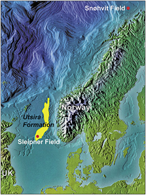
Figure 1. Location map of Sleipner Project showing the Utsira formation extent (after Arts et al., 2008).

The Sleipner Project injected supercritical CO₂ at a depth of 1,012 m into the saline aquifer of the Utsira Formation Sandstone (Arts et al., 2008), which has a favorable porosity of 35%–40% to store CO₂, adequate for applying seismic monitoring techniques (Eiken et al., 2011). Under favorable conditions, CO₂ monitoring has been successful in the Sleipner Project (Arts et al., 2003; Arts et al., 2008; Chadwick et al., 2010). Additional quantitative analyses of time-lapse seismic data are ongoing using a wide-scope approach. Time-lapse seismic data, also known as 4D seismic imaging, represents a sophisticated geophysical monitoring technique that captures sequential seismic surveys of the same geological formation over multiple time intervals. This method enables the detection and quantification of subtle changes in subsurface characteristics, particularly crucial in CCS and hydrocarbon reservoir monitoring. The depth interval of CCS storage on time-lapse seismic data that includes some heterogeneities with thin layers is of particular interest for developing research that would be valuable to the post-injection stages (White et al., 2018a; Izadian, 2024).

Seven vintage seismic surveys were conducted, starting with a baseline survey in 1994 and continuing in 1999, 2001, 2004, 2006, 2008, and 2010 (Furre et al., 2017). Time-lapse data were released in January 2020 (Sleipner 4D Seismic Database, 2020), consisting of migrated volumes and velocity maps that can be converted into depth-domain data. The seismic volume and acquisition parameters used here are listed in Table 1, which shows consistency with the vintage surveys.

Table 1

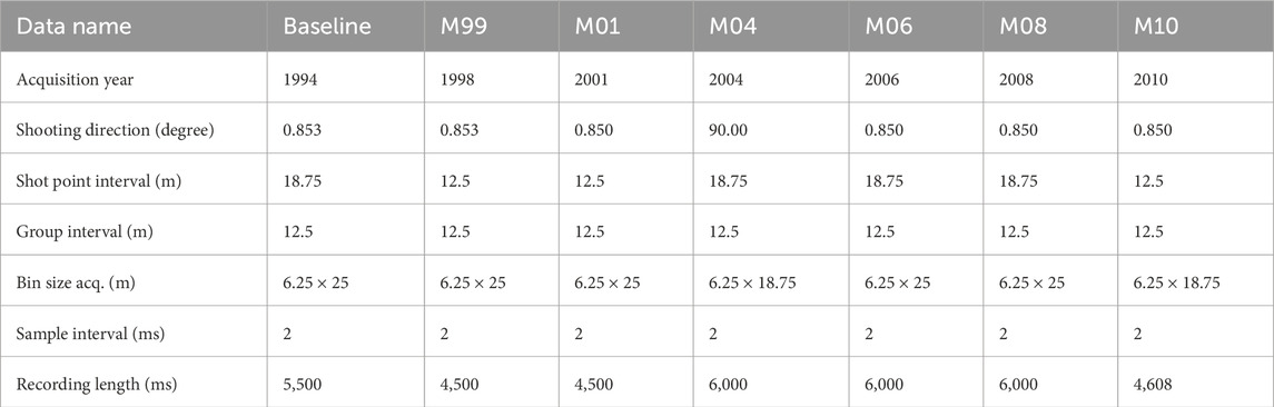
Table 1. Survey data list and acquisition parameters.

All time-lapse seismic datasets show sufficient resolution to enable imaging of the amplitude difference from 4D processing (Williams and Chadwick, 2012). The bin size along the survey was 6.25 m and less than 25 m across, which enabled 4D seismic monitoring with a good resolution. The frequency range of seismic data is between 15 Hz and 55 Hz, centered at 35 Hz, with a tuning thickness of 14 ms in two-way travel time. This resolution enhances layer heterogeneity decomposition and derives confident velocity information (Chadwick et al., 2019). To further validate the seismic data, additional information contained in the seismic attributes was utilized to obtain more amplitude-varying features.

2.2 Attribute analysis and volume calculation

There are various seismic attributes in the Sleipner dataset. To analyze these, the IHS Kingdom™ Suite software was used, which provides intrinsic attributes in four categories: wavelet, instantaneous, geometric, and stratigraphic. Among the available attributes, the trace envelope (TE) is preferred for identifying CO₂ plumes. TE, also known as instantaneous amplitude, can be calculated using the absolute value of the function amplitude. It involves all positive values that may represent the individual interface contrast so that it can highlight anomalous regions.

When the original seismic trace $f\left(z\right)$ is obtained, TE (Equation 1) can be written as

$\mathit{T}\mathit{E}\left(\mathit{z}\right)=\sqrt{{\left[\mathit{R}\mathit{e}\left(\mathit{f}\left(\mathit{z}\right)\right)\right]}^{\mathbf{2}}+{\left[\mathit{I}\mathit{m}\left(\mathit{f}\left(\mathit{z}\right)\right)\right]}^{\mathbf{2}}}(1)$

where $Re\left(f\left(z\right)\right)$ and $Im\left(f\left(z\right)\right)$ are the real and imaginary parts of the Hilbert transform of the seismic trace, respectively (Taner et al., 1979). Because TE has only a positive magnitude, a subtle polarity change in the spatial domain would be blurred or neglected. Instead, the amplitude differences near the CO₂ plume injection region were highlighted. We intend to design additional new attributes that should minimize amplitude changes in the background region and further maximize the effect of discriminating amplitude anomalies.

The similarity variance (SV) value is an additional attribute consistent with a similar lithology. If the interval is saturated with CO₂, a similar interval is expected. Therefore, similarity (Equation 2) was used as a secondary attribute, expressed as shown below:

$\mathit{S}\left(\mathit{z}\right)=\frac{{\displaystyle {\sum }_{\mathit{\tau }=-\mathit{N}/\mathbf{2}}^{\mathit{\tau }=\mathit{N}/\mathbf{2}}}{\left\{{\displaystyle {\sum }_{\mathit{m}=\mathbf{1}}^{\mathit{M}}}{\mathit{f}}_{\mathit{m}}\left(\mathit{z}+\mathit{\tau }\right)\right\}}^{\mathbf{2}}}{{\displaystyle {\sum }_{\mathit{\tau }=-\mathit{N}/\mathbf{2}}^{\mathit{\tau }=\mathit{N}/\mathbf{2}}}{\displaystyle {\sum }_{\mathit{m}=\mathbf{1}}^{\mathit{M}}}{\mathit{f}}_{\mathit{m}}^{\mathbf{2}}\left(\mathit{z}+\mathit{\tau }\right)}(2)$

where f_m(z) is the mth trace of the gather, N is the length of the computational window in both time and depth domains, and z represents either time or depth. This is also the calculation of semblance property, which represents a measure of the coherent power existing between several traces versus the total power of all traces. Next, the variance of similarity (Equation 3) was calculated:

$\mathit{S}\mathit{V}=\mathit{E}\left[{\left(\mathit{S}-{\mathit{S}}_{\mathit{m}\mathit{e}\mathit{a}\mathit{n}}\right)}^{\mathbf{2}}\right](3)$

where S is the similarity, S_mean is the mean value of S, and E is the expectation of S. Therefore, the SV calculated by the expected value of the squared deviation from the mean of similarity represents local anomalies with respect to the smoothed averaged background. By including the similarity variance in the exponential function so that a smaller SV represents a higher anomaly following high coherency events, the CO₂ plume region was easier to distinguish.

To merge the relative attributes into a new one, the data trend was inspected. The new attribute CO2IDC—an indicator of carbon dioxide—Equation 4 was calculated as shown below:

$\mathit{C}\mathit{O}\mathbf{2}\mathit{I}\mathit{D}\mathit{C}=\mathit{T}\mathit{E}\left(\mathit{z}\right)·{\mathit{e}}^{{-\left(\frac{\mathit{S}\mathit{V}}{\mathbf{2}}\right)}^{\mathbf{2}}}(4)$

Here, CO2IDC is a property of the corrected TE obtained by adding the damping effect of the SV weighting to minimize the local variance from the plume area. We expect that CO2IDC can distinguish the CO₂ plume region from the TE. Using these attributes, we commenced matching by displaying the relevant vertical and horizontal sections with the vintage surveys. The plume area was then captured using a polygon boundary. The time-lapse plume area correlated with the amount of CO₂ injected into the Sleipner field. This is the first correlation of quantitative matching that uses two-dimensional interpretation results in the workflow (Figure 2). The subsequent correlations are the matching amount of injected CO₂ with the three-dimensional plume volume interpreted by the attributes of TE and CO2IDC. The most important factor in determining these attributes is the area of the plume region interpreted on the seismic time-slice map. We calculated the area of the plume region by changing the moving width size in TE and SV computations, and the Sleipner data had a sensitivity of about 3% (Table 2). This value means that consistent plume area calculations are possible, and therefore, the method using CO2IDC would have robustness.

Figure 2

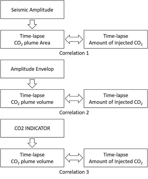
Figure 2. Flow chart on quantitative matching of CO₂ amount via seismic attributes.

Table 2

Table 2. Sensitivity analysis between the polygon selection and the moving window width.

The spatial volume of the CO₂ plume was calculated from the two-dimensional interpretation results to input the quantitative matching. Previous studies using the Sleipner dataset have reported that the plume extends over nine layers (Boait et al., 2012; Chadwick and Noy, 2015). For volume calculation, the average value was used after calculating the volume of the area occupied by the polygons of the grid top and bottom layers, without separately calculating all layers for efficiency (Figure 3). This method would be effective in excluding the influence of the thin-bed tuning effect that researchers are concerned about (Izadian, 2024). The plume area of top and bottom was computed by summation of polygons that can be assigned inner boundaries from plume top and bottom interpretation. To convert the time-domain seismic data into a spatial grid, the velocity map for each layer provided by the Sleipner Project was input (Sleipner 4D Seismic Dataset, 2020). A volume calculator in Kingdom™ was used to determine the volume of the polygon area occupied vertically by the top and bottom layers. In summary, the volume calculation method consists of calculating the area (top and bottom) boundary with a polygon, converting the time-domain seismic data into a space grid using a velocity map, and deriving the total plume’s volume value. These operations were applied to polygons using TE and CO2IDC, and plume volumes were calculated for all seismic datasets for each acquisition period (Baseline, M99, M01, M04, M06, M08, and M10).

Figure 3

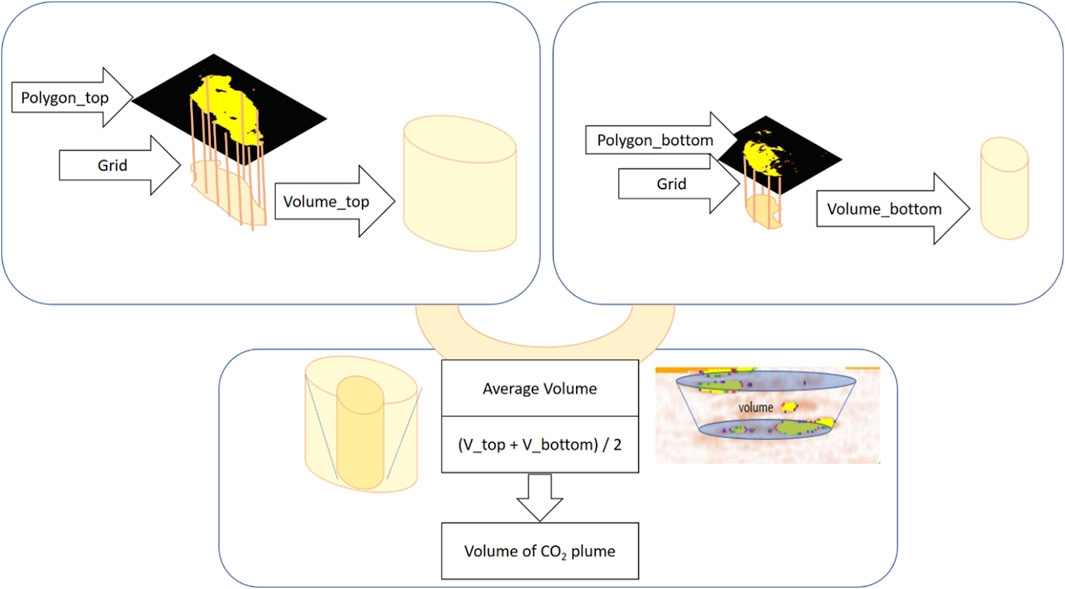
Figure 3. Volume calculation for the CO₂ plume region between the top and bottom layers.

3 Results and discussion

3.1 Matching CO₂ amount with primary seismic amplitude

The amount of injected CO₂ was matched against the plume area inferred from seismic data to validate the usage of primary seismic amplitude data. A seismic section is depicted at the inline, crossline vertical section, and time-slice on the horizontal map to compare the matching results. The area of CO₂ was determined via a manual selection of the plume boundary on the time-slice map. Then, a crossplot between the area and injected CO₂ volume was used to obtain a regression degree of fitting.

After loading seismic data, four horizons were interpreted: mean sea level, top sand wedge, and top and bottom Utsira Formation. The CO₂ plume lies between orange and green, as indicated in Figure 4, where the interval between the top and bottom Utsira Formation is located. All seven vertical sections are depicted at inline 1830, close to the center of the survey area adjacent to the location of the injection point. In the baseline data, there was no anomaly between the orange and green horizons (Figure 4a). As the amount of injected CO₂ increased, the anomalous event exhibited a CO₂ plume growth (Figures 4b–g). Figure 4h shows the corresponding position in the map view.

Figure 4

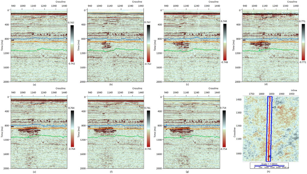
Figure 4. Representative vertical sections in shooting directions with time-lapse seismic volumes: (a) baseline; (b) M99; (c) M01; (d) M04; (e) M06; (f) M08; (g) M10; (h) map view of the seismic line.

The growth of the CO₂ plume can be clearly seen when displayed on a time-slice map. Depicted maps at 0.95 ms two-way travel time (TWTT)―representing the depth of the top Utsira Formation―were displayed and used to select the plume region (Figure 5). The increase in the plume area with time-lapse on the map represents almost 1 million tons of CO₂ injected annually. The anomaly aspect is displayed in red and black, indicating negative and positive amplitude changes, respectively. The boundary of the anomalous area was selected on the time-slice map, and the area of the CO₂ plume was estimated.

Figure 5

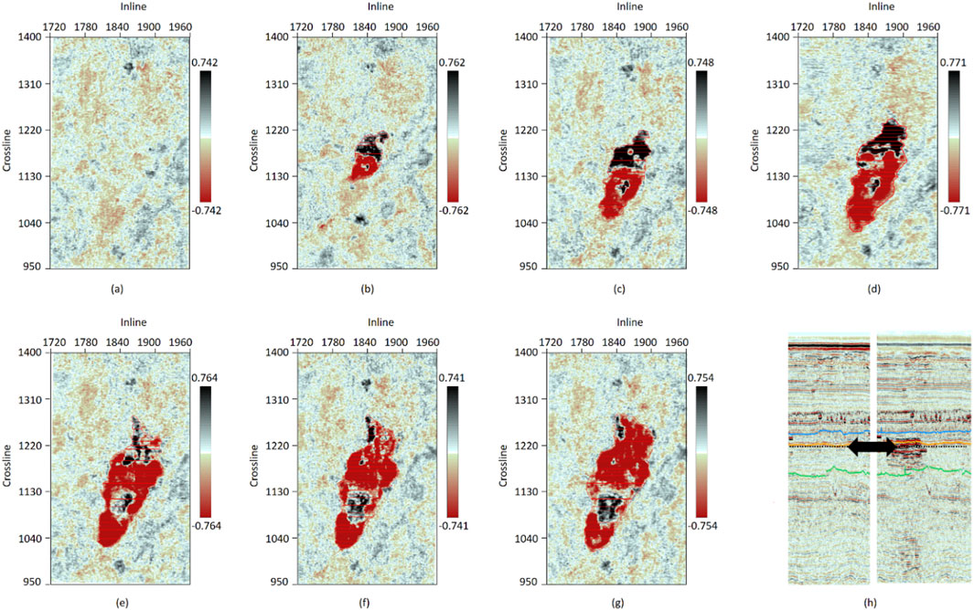
Figure 5. Representative time-slice map at 0.950 ms travel time depth of time-lapse seismic volumes: (a) baseline; (b) M99; (c) M01; (d) M04; (e) M06; (f) M08; (g) M10; (h) seismic line of the baseline survey (left, Figure 4a) and the M10 survey (right, Figure 4g) in section view with arrows indicating the depth of the corresponding time-slices.

According to the Sleipner 4D Seismic Database (2020), the amount of injected CO₂ is approximately one million tons per year. The cumulative amount of CO₂ is listed in Table 3. The area of the CO₂ plume boundary was calculated using the polygon tool in the time-slice map at 0.950 ms travel time depths and compared with the injected CO₂ amount. As indicated in Figure 6, the crossplot shows a good correlation between CO₂ amount and the calculated area of the plume determined at the time-slice, proving that the Sleipner time-lapse dataset records the CO₂ plume growth quantitatively. As observed with seismic amplitude only, the CO₂ plume growth correlates with a CO₂ injection increase. The correlation is high (0.9895), as the amount of CO₂ is quite large, and the area expands over a large range.

Table 3

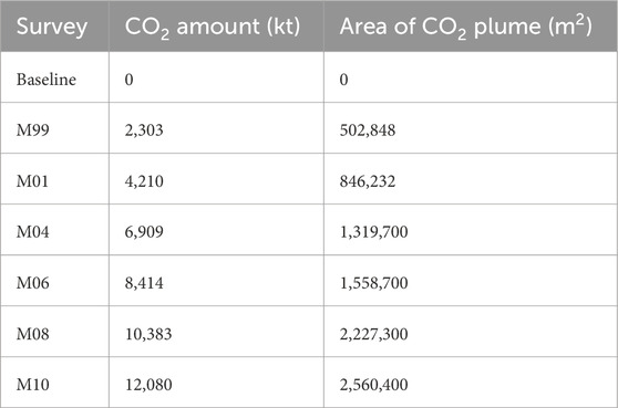
Table 3. Matching amount of CO₂ with plume area from the time-slice map at a depth of TWTT 0.95 ms.

Figure 6

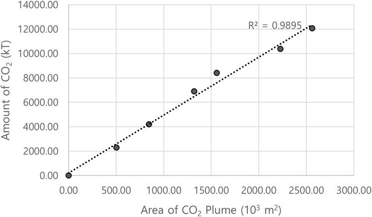
Figure 6. Matching amount of CO₂ with CO₂ plume area calculated by the seismic reflection amplitude.

An injection volume proportional to the CO₂ plume area can be justified if the thickness is constant and there is no change in the upper and lower areas. In actual field conditions, the area where CO₂ spreads is different for each layer; therefore, more accurate matching is possible if this is considered. Because it is obvious that the volume of stored CO₂ increases as the injection amount increases, the assessment of the correlation must be precisely quantified with the upper and lower plume boundaries to perform accurate monitoring. Therefore, the correlation between secondary seismic attributes and the amount of CO₂ was quantified, particularly focusing on the discrimination of the lower CO₂ boundary, which is not clearly revealed on seismic amplitude.

3.2 Quantification of CO₂ by secondary seismic attributes

Although the primary seismic amplitude shows a clear image of the CO₂ plume in the Utsira Formation, the lower part of the plume has a smaller area, making recognition harder than the upper part of the plume boundary. To determine the volume of the CO₂ plume region, additional seismic attributes can help distinguish between anomalous regions with background storage formation.

The TE of the Sleipner seismic data represents all positive values at every time sample, especially the anomaly in yellow in Figure 7, which shows an anomalous stored CO₂ region in the Utsira Formation. This facilitated the identification of the CO₂ plume in the vertical dimension. The visually observed CO₂ plume region was similar in the primary amplitude of the seismic data and in the secondary TE attribute data. To determine the plume volume in three dimensions, it was established that TE is advantageous for selecting the amplitude boundary on a time-slice map. To calculate the CO₂ plume volume, the average of two cylinders from the top and bottom selected layer boundaries was used (Figure 8). The top of the Utsira Formation was selected at 0.950 ms TWTT on the TE map (Figures 8a–e), showing a similar boundary with seismic amplitude (Figures 5b–f). Interpretation of the bottom Utsira Formation shows less area as seen on amplitude selections from the CO₂ saturation region on the TE time-slice (Figures 8f–j).

Figure 7

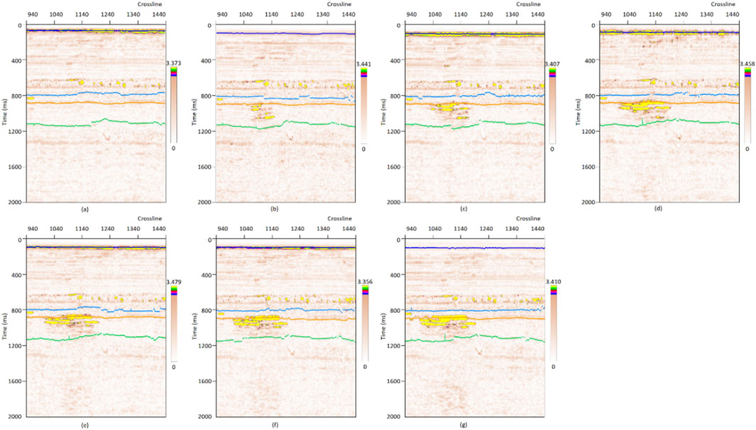
Figure 7. Representative vertical sections of TE attributes in shooting directions with time-lapse seismic volumes: (a) baseline; (b) M99; (c) M01; (d) M04; (e) M06; (f) M08; (g) M10.

Figure 8

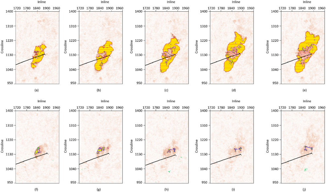
Figure 8. Representative time-slice map of TE at 0.950 ms TWTT at the depth of the upper plume boundaries for (a) M99; (b) M01; (c) M04; (d) M06; (e) M08 data, and at 1.050 ms TWTT of the lower plume boundaries for (f) M99; (g) M01; (h) M04; (i) M06; (j) M08.

The result of the matching between the plume volume calculated by TE and the injected amount of CO₂ is shown in Table 4. The regression value decreased from 0.9895 to 0.9690 as it was affected by the inaccurate selection of the bottom area (Figure 9). This regression value is not unique because it is determined by a manually selected result for the upper and lower area boundaries. Obtaining an accurate selection method is dependent on the seismic resolution. With the Sleipner data, the resolution of the seismic volume is fairly good; thus, it is easy to select an anomalous event. However, in the case of a degraded time-lapse seismic dataset, it is difficult to select a CO₂ plume boundary that worsens the matching quality for monitoring CO₂. The difficulties in determining the bottom Utsira Formation are consistent when the selection is made on the primary seismic amplitude. Thus, it is a major trigger for introducing additional attributes that represent the CO₂ plume region.

Table 4

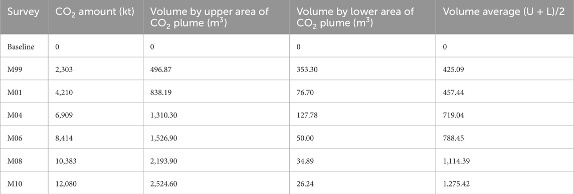
Table 4. Matching CO₂ amount with volume calculated by TE attributes at a depth between time-slice maps at 0.95 ms and 1.05 ms.

Figure 9

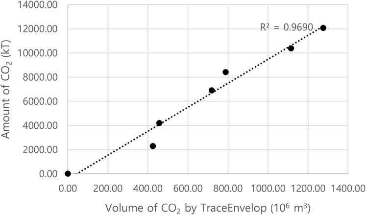
Figure 9. Matching amount of CO₂ with the volume of the CO₂ plume region calculated by the TE attribute.

As introduced previously, CO2IDC was calculated and displayed using the Sleipner dataset (Figure 10). Because CO2IDC is calculated from the TE and weighted by the exponential value of SV, it is similar to the TE section. In the vertical section, CO2IDC can more easily differentiate the CO₂ plume anomaly from the background area because the signal amplitude is manipulated by TE and SV to maximize coherence.

Figure 10

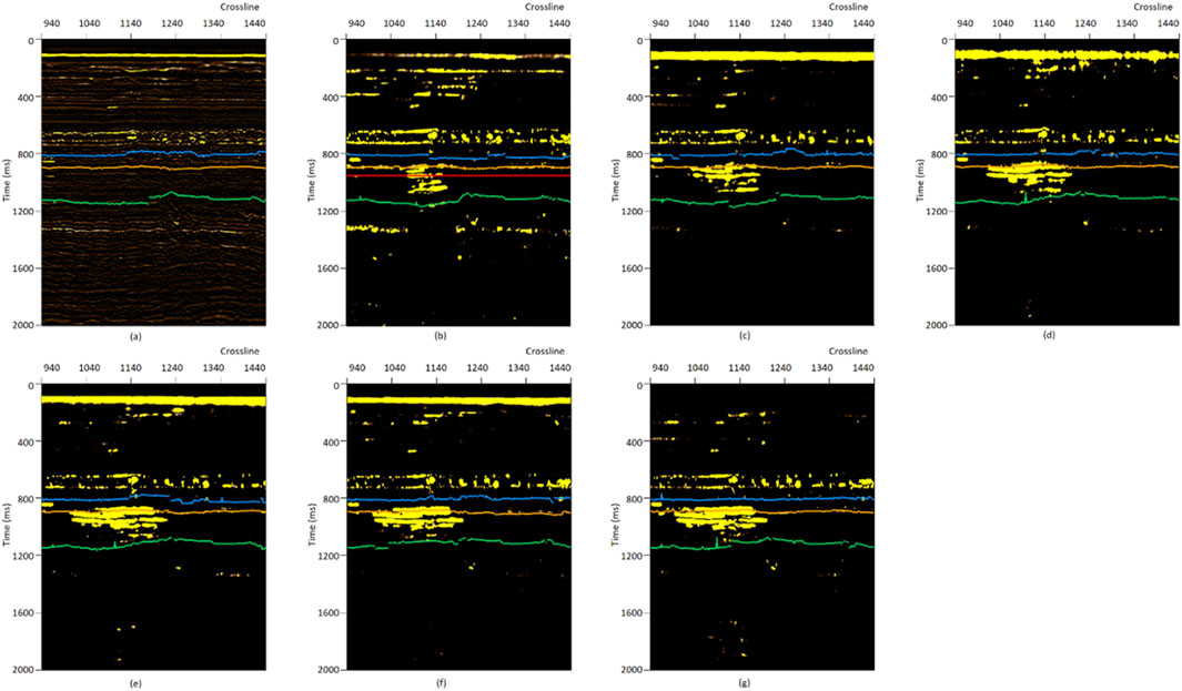
Figure 10. Representative vertical sections of the CO2IDC attribute in shooting directions with time-lapse seismic volumes at (a) baseline, (b) M99; (c) M01; (d) M04; (e) M06; (f) M08; (g) M10.

The CO2IDC on the time-slice map shows the difference in the CO₂ plume region more clearly, making it easier to select the boundary. In particular, the lower boundary of the CO₂ plume was recognized with the background Utsira Formation (Figure 11). This is an advantage of using the additional attribute of CO2IDC, which was specifically designed for the Sleipner dataset. The matching values between the injected CO₂ and the plume volume calculated by CO2IDC are listed in Table 5. The values of the CO₂ volumes, calculated by the lower layer cylinder, tend to be consistent, implying that the selection results of the boundary are robust along the time-lapse data. Figure 12 shows the crossplot of the matching result between the amount of CO₂ and plume volume as calculated by the CO2IDC. The regression value increased to 0.9906, indicating the validity of the attribute manipulation.

Figure 11

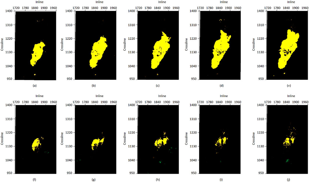
Figure 11. Representative time-slice map of CO2IDC at 0.950 ms travel time depth of seismic volumes: (a) M99; (b) M01; (c) M04; (d) M06; (e) M08, and at 1.050 ms (f) M99; (g) M01; (h) M04; (i) M06; (j) M08.

Table 5

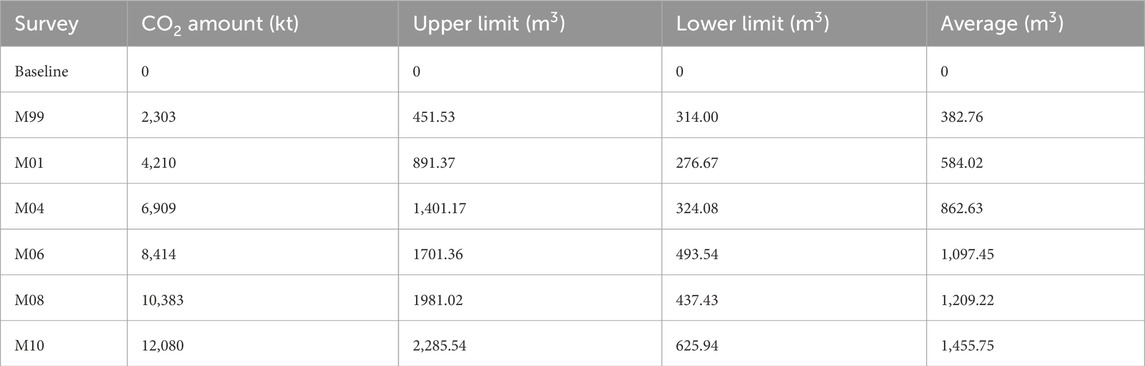
Table 5. Matching CO₂ amount with volume calculated by CO2IDC.

Figure 12

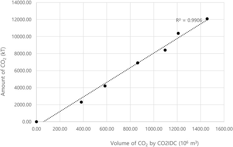
Figure 12. Matching amount of CO₂ with the volume of the CO₂ plume region as calculated by the CO2IDC attribute.

3.3 Discussion

We selected a high-resolution seismic dataset released by the Sleipner Project that provides the best quality time-lapse seismic data. The data show an anomaly that is sufficiently large to detect CO₂ qualitatively and has been proven by previous researchers (e.g., Arts et al., 2008; Furre et al., 2017). Previous work has confirmed the feasibility of quantifying injected CO₂ with respect to seismic data, showing that anomalous amplitude is related to the amount of CO₂, especially via layers on seismic images (Chadwick et al., 2009; Chadwick et al., 2010). CO₂ saturation is evaluated on a subsequent study utilizing seismic and rock physics inversion (Dupuy et al., 2017b). This quantification through inversion determined the CO₂ saturation with high accuracy, and such efforts will be repeated using time-lapse data. The pre-stack inverted impedance also showed highly reliable results for CO₂ saturation (Rasolofosaon and Dubos-Sallee, 2010). The method used here is merit worthy as it is less time-consuming than other methods, such as seismic inversion. More possibilities remain to be quantified, including monitoring issues dealing with history matching with CO₂ amounts (Williams and Chadwick, 2017; White et al., 2018b). Conventional studies of history matching focus on well log data that are direct and accurate but make limited use of seismic data (Yin et al., 2019; Ahmadinia and Shariatipour, 2020).

From another viewpoint, we accept seismic attributes to determine the feasibility of historical matching with seismic data in the case of a limited availability of well logs. A seismic attribute is a standalone piece of information that can provide physical properties with high confidence and degree of freedom. However, the selection of an attribute is based on a data evaluation. In this case, the amount of CO₂ is large; thus, the correlation of matching should be measured accurately. Building a new attribute is necessary to enhance time-lapse seismic data utilization, for example, to address pressure changes or to monitor porosity. Because the growth of the plume is not always consistent with the seismic interpretation, the detailed relationship between seismic signals and fluid substitution should be investigated.

In particular, stored CO₂ is a fluid, so it can migrate over time, and especially in the case of faults, it must be monitored with fluid migration mechanisms. The flow of CO₂ along complex strata and fracture zones is partially tracked in time-lapse seismic studies, and the CO2IDC presented in this study was introduced to confirm this more easily. However, it is desirable to utilize geochemical tracer studies as a method to directly and reliably track the flow of fluid (Buttitta et al., 2020; Caracausi et al., 2022). These methods have the advantage of being able to identify detailed fluid flow when included in the design process of a CCS project. It is also a method that can be applied cost-effectively compared to repeated seismic surveys. In case of geophysical data only, our method verifies CO₂ accommodation with attributes that were already confirmed with a slowly migrating plume without large-scale faults on the Sleipner data that were already published.

In time-slices corresponding to 1.05 ms of CO2IDC in the M04, M06, and M08 data, we identified a separated plume area boundary corresponding to a reported chimney event (Karstens et al., 2017; Williams and Chadwick, 2017). With only the seismic amplitude, the CO₂ charged region was ambiguous because of positive and negative wiggling. This study proves that the specific interest in stored CO₂ plumes can be investigated more easily by designing seismic attributes. However, there remains a validation limitation when challenging data are available. Because the present CO2IDC was designed by empirical determination, engaging other datasets would require a different damping value. In particular, when monitoring using seismic attributes is applied to heterogeneous, faulted, or fluid-rich geological domains, additional background information such as geochemical or geological interpretation should be utilized (Buttitta et al., 2023; Zummo et al., 2024). If experiences and case studies on various datasets accumulate, it will be possible to convert and standardize such information into quantifiable attributes. If active technologies such as machine learning, which have been in the spotlight recently, are utilized, the feasibility of the application will be secured more easily. Future studies may focus on the robust selection of attributes, regardless of data characteristics. If we achieve non-biased data analysis, the result of manipulating attributes for quantifying subsurfaces can be used across other disciplines, such as in monitoring aquifer pressure change, in addition to the CCS field.

4 Conclusion

Here, we analyzed a seismic attribute that can monitor CO₂ amounts more effectively than the seismic amplitude itself. The trace envelope (TE) showed the CO₂ plume region clearly with respect to time. The advantage of using a TE is that it has all positive values; therefore, it instinctively describes the plume boundary. The plume volume was estimated from the TE and was positively correlated with the amount of CO₂ injected into the Utsira Formation. To improve the correlation between the injected CO₂ amount and volume by seismic aspect, we designed a new CO₂ indicator attribute based on the TE and similarity variance. The attribute of the CO₂ indicator discriminated the CO₂ saturated region qualitatively. The regression value increase in the correlation between the CO₂ amount and volume calculated by CO2IDC proves that seismic attributes can be used to monitor CO₂ for efficient CCS. Attributes analysis with a time-lapse scale can enhance the usage of Sleipner data and promote more intense research for CCS in general.

Data availability statement

Publicly available datasets were analyzed in this study. These data can be found here: https://co2datashare.org/dataset.

Author contributions

SC: Conceptualization, Data curation, Methodology, Writing – original draft, Writing – review and editing. SY: Formal analysis, Supervision, Writing – review and editing. VS: Conceptualization, Writing – review and editing.

Funding

The author(s) declare that financial support was received for the research and/or publication of this article. “Technology development for storage efficiency improvement and safety assessment of CO₂ geological storage (24-3413)” and “Development of offshore CO₂ monitoring technology and transboundary CCUS business models through participation in Australian project (24-4863)” at the Korea Institute of Geoscience and Mineral Resources (KIGAM).

Acknowledgments

The authors would like to thank reviewers for taking the time and effort necessary to review the manuscript.

Conflict of interest

The authors declare that the research was conducted in the absence of any commercial or financial relationships that could be construed as a potential conflict of interest.

Publisher’s note

All claims expressed in this article are solely those of the authors and do not necessarily represent those of their affiliated organizations, or those of the publisher, the editors and the reviewers. Any product that may be evaluated in this article, or claim that may be made by its manufacturer, is not guaranteed or endorsed by the publisher.

References

Ahmadinia, M., and Shariatipour, S. M. (2020). Analysing the role of caprock morphology on history matching of Sleipner CO₂ plume using an optimisation method. Greenh. Gases Sci. Technol. 10, 1077–1097. doi:10.1002/ghg.2027

CrossRef Full Text | Google Scholar

Ahmadinia, M., Shariatipour, S. M., Andersen, O., and Nobakht, B. (2020). Quantitative evaluation of the joint effect of uncertain parameters in CO₂ storage in the Sleipner project, using data-driven models. Int. J. Greenh. Gas Control 103, 103180. doi:10.1016/j.ijggc.2020.103180

CrossRef Full Text | Google Scholar

Arts, R., Chadwick, A., Eiken, O., Thibeau, S., and Nooner, S. (2008). Ten years’ experience of monitoring CO₂ injection in the Utsira Sand at Sleipner, offshore Norway. First Break 26, 65–72. doi:10.3997/1365-2397.26.1115.27807

CrossRef Full Text | Google Scholar

Arts, R., Eiken, O., Chadwick, A., Zweigel, P., van der Meer, L., and Zinszner, B. (2003). “Monitoring of CO₂ injected at Sleipner using time lapse seismic data,” in Proceedings of the 6th International Conference on Greenhouse Gas Control, Kyoto, Japan, October 1–4.

Google Scholar

Bachu, S. (2015). Review of CO₂ storage efficiency in deep saline aquifers. Int. J. Greenh. Gas Control 40, 188–202. doi:10.1016/j.ijggc.2015.01.007

CrossRef Full Text | Google Scholar

Behrens, R. A., MacLeod, M. K., Tran, T. T., and Alimi, A. O. (1998). Incorporating seismic attribute maps in 3D reservoir models. SPE Reserv. Eval. & Eng. 1, 122–126. doi:10.2118/36499-pa

CrossRef Full Text | Google Scholar

Benson, S. M., Bennaceur, K., Cook, P., Davison, J., de Coninck, H., Farhat, K., et al. (2012). “Carbon capture and storage,” in Global Energy assessment- toward a sustainable future, 993. Cambridge, United Kingdom: Cambridge University Press.

Google Scholar

Boait, F. C., White, N. J., Bickle, M. J., Chadwick, R. A., Neufeld, J. A., and Huppert, H. E. (2012). Spatial and temporal evolution of injected CO2 at the Sleipner field, North Sea. J. Geophys. Res. 117, B03309. doi:10.1029/2011JB008603

CrossRef Full Text | Google Scholar

Buttitta, D., Capasso, G., Paternoster, M., Barberio, M. D., Gori, F., Petitta, M., et al. (2023). Regulation of deep carbon degassing by gas-rock-water interactions in a seismic region of Southern Italy. Sci. Total Environ. 897, 165367. doi:10.1016/j.scitotenv.2023.165367

PubMed Abstract | CrossRef Full Text | Google Scholar

Buttitta, D., Caracausi, A., Chiaraluce, L., Favara, R., Gasparo Morticelli, M., and Sulli, A. (2020). Continental degassing of helium in an active tectonic setting (northern Italy): the role of seismicity. Sci. Rep. 10 (1), 162. doi:10.1038/s41598-019-55678-7

PubMed Abstract | CrossRef Full Text | Google Scholar

Caracausi, A., Buttitta, D., Picozzi, M., Paternoster, M., and Stabile, T. A. (2022). Earthquakes control the impulsive nature of crustal helium degassing to the atmosphere. Commun. Earth & Environ. 3 (1), 224. doi:10.1038/s43247-022-00549-9

CrossRef Full Text | Google Scholar

Chadwick, R. A. (2013). “Offshore CO₂ storage: Sleipner natural gas field beneath the North Sea,” in Geological storage of carbon dioxide. CO₂ (Amsterdam, Netherlands: Elsevier), 227–253e. doi:10.1533/9780857097279.3.227

CrossRef Full Text | Google Scholar

Chadwick, R. A., Noy, D., Arts, R., and Eiken, O. (2009). Latest time-lapse seismic datafrom Sleipner yield new insights into CO₂ plume development. Energy Procedia 1, 2103–2110. doi:10.1016/j.egypro.2009.01.274

CrossRef Full Text | Google Scholar

Chadwick, R. A., and Noy, D. J. (2010). History matching flow simulations and time-lapse seismic data from the Sleipner CO₂ plume. Pet. Geol. Conf. Ser. 7, 1171–1182. doi:10.1144/0071171

CrossRef Full Text | Google Scholar

Chadwick, R. A., and Noy, D. J. (2015). Underground CO₂ storage: demonstrating regulatory conformance by convergence of history-matched modeled and observed CO₂ plume behavior using Sleipner time-lapse seismics. Greenh. Gases Sci. Technol. 5, 305–322. doi:10.1002/ghg.1488

CrossRef Full Text | Google Scholar

Chadwick, R. A., Williams, G., Delepine, N., Clochard, V., Labat, K., Sturton, S., et al. (2010). Quantitative analysis of time-lapse seismic monitoring data at the Sleipner CO₂ storage operation. Lead. Edge 29, 170–177. doi:10.1190/1.3304820

CrossRef Full Text | Google Scholar

Chadwick, R. A., Williams, G. A., and Falcon-Suarez, I. (2019). Forensic mapping of seismic velocity heterogeneity in a CO₂ layer at the Sleipner CO₂ storage operation, North Sea, using time-lapse seismics. Int. J. Greenh. Gas Control 90, 102793. doi:10.1016/j.ijggc.2019.102793

CrossRef Full Text | Google Scholar

Chen, Q., and Sidney, S. (1997). Seismic attribute technology for reservoir forecasting and monitoring. Lead. Edge 16, 445–448. doi:10.1190/1.1437657

CrossRef Full Text | Google Scholar

Cho, Y., and Jun, H. (2021). Estimation and uncertainty analysis of the CO₂ storage volume in the Sleipner field via 4D reversible-jump markov-chain Monte Carlo. J. Petroleum Sci. Eng. 200, 108333. doi:10.1016/j.petrol.2020.108333

CrossRef Full Text | Google Scholar

Chopra, S., and Marfurt, K. J. (2005). Seismic attributes- A historical perspective. Geophysics 70, 3SO–28SO. doi:10.1190/1.2098670

CrossRef Full Text | Google Scholar

Dupuy, B., Romdhane, A., Eliasson, P., Querendez, E., Yan, H., Torres, V. A., et al. (2017a). Quantitative seismic characterization of CO₂ at the Sleipner storage site, North Sea. Interpretation 5, SS23–SS42. doi:10.1190/int-2017-0013.1

CrossRef Full Text | Google Scholar

Dupuy, B., Torres C, V. A., Ghaderi, A., Querendez, E., and Mezyk, M. (2017b). “Constrained AVO for CO₂ storage monitoring at Sleipner,” in Proceedings of the 13th International Conference on Greenhouse Gas Control, Lausanne, Switzerland, November 14–18.

Google Scholar

Eiken, O., Ringrose, P., Hermanrud, C., Nazarian, B., Torp, T., and Hoier, L. (2011). Lessons learned from 14 years of CCS operations: Sleipner, in Salah and Snohvit. Energy Procedia 4, 5541–5548. doi:10.1016/j.egypro.2011.02.541

CrossRef Full Text | Google Scholar

Furre, A., Eiken, O., Alnes, H., Vevatne, J. N., and Kiaer, A. F. (2017). 20 years of monitoring CO2-injection at Sleipner. Energy Procedia 114, 3916–3926. doi:10.1016/j.egypro.2017.03.1523

CrossRef Full Text | Google Scholar

Ghosh, R., Sen, M. K., and Vedanti, N. (2015). Quantitative interpretation of CO₂ plume from Sleipner (North Sea), using post-stack inversion and rock physics modeling. Int. J. Greenh. Gas Control 32, 147–158. doi:10.1016/j.ijggc.2014.11.002

CrossRef Full Text | Google Scholar

Goloshubin, G., Silin, D., Vingalov, V., Takkand, G., and Latfullin, M. (2008). Reservoir permeability from seismic attribute analysis. Lead. Edge 27 (3), 376–381. doi:10.1190/1.2896629

CrossRef Full Text | Google Scholar

Gori, F., Paternoster, M., Barbieri, M., Buttitta, D., Caracausi, A., Parente, F., et al. (2023). Hydrogeochemical multi-component approach to assess fluids upwelling and mixing in shallow carbonate-evaporitic aquifers (Contursi area, southern Apennines, Italy). J. Hydrology 618, 129258. doi:10.1016/j.jhydrol.2023.129258

CrossRef Full Text | Google Scholar

Gozalpour, F., Ren, S. R., and Tohidi, B. (2005). CO₂ EOR and storage in oil reservoirs. Oil & Gas Sci. Technol. 60, 537–546.

Google Scholar

Haffinger, P., Doulgeris, P., and Gisolf, A. (2017). “Quantitative seismic reservoir monitoring by using a wave-equation based AVO technology,” in 1st EAGE Workshop on Practical Reservoir Monitoring, Amsterdam, Netherlands, March 06–09.

Google Scholar

Haffinger, P., Eyvazi, F. J., Steeghs, T. P. H., Doulgeris, P., and Gisolf, A. (2016). “Quantitative prediction of injected CO₂ at Sleipner using wave-equation based AVO,” in Proceedings of 78th EAGE Conference and exhibition, Vienna, Austria, May 30–June 2.

Google Scholar

Hannis, S., Chadwick, A., Pearce, J., Jones, D., White, J., Wright, I., et al. (2015). Review of offshore monitoring for CCS Projects. Cheltenham, UK: IEAGHG.

Google Scholar

Hart, B. S. (2002). Validating seismic attribute studies: beyond statistics. Lead. Edge 21, 1016–1021. doi:10.1190/1.1518439

CrossRef Full Text | Google Scholar

Hema, G., Maurya, S. P., Kant, R., Singh, A. P., Verma, N., Sing, R., et al. (2024). Enhancement of CO2 monitoring in the Sleipner field (north sea) using seismic inversion based on simulated annealing of time-lapse seismic data. Mar. Petroleum Geol. 167, 106962. doi:10.1016/j.marpetgeo.2024.106962

CrossRef Full Text | Google Scholar

IPCC (2005). Carbon dioxide capture and storage. in Special Report of the Intergovernmental Panel on Climate Change. Editors B. Metz, O. Davison, H. C. de COnick, M. Loos, and L. A. Meyer (Cambridge, United Kingdom: Cambridge University Press), 442.

Google Scholar

Izadian, S. (2024). Tuning effect in time-lapse seismic inversion for CO2 plume monitoring at Sleipner field. Int. J. Greenh. Gas Control 137, 104224. doi:10.1016/j.ijggc.2024.104224

CrossRef Full Text | Google Scholar

Karstens, J., Ahmed, W., Berndt, C., and Class, H. (2017). Focused fluid flow and the sub-seabed storage of CO2: evaluating the leakage potential of seismic chimney structures for the Sleipner CO2 storage operation. Mar. Petroleum Geol. 88, 81–93. doi:10.1016/j.marpetgeo.2017.08.003

CrossRef Full Text | Google Scholar

Marfurt, K. J., and Alves, T. M. (2015). Pitfalls and limitations in seismic attribute interpretation of tectonic features. Interpretation 3, SB5–SB15. doi:10.1190/int-2014-0122.1

CrossRef Full Text | Google Scholar

Massarweh, O., and Abushaikha, A. S. (2024). CO2 sequestration in subsurface geological formations: a review of trapping mechanisms and monitoring techniques. Earth-Science Rev. 253, 104793. doi:10.1016/j.earscirev.2024.104793

CrossRef Full Text | Google Scholar

Raknes, E. B., Arntsen, B., and Weibull, W. (2015). Three-dimensional elastic full waveform inversion using seismic data from the Sleipner area. Geophys. J. Int. 202, 1877–1894. doi:10.1093/gji/ggv258

CrossRef Full Text | Google Scholar

Rasolofosaon, P. N. J., and Dubos-Sallee, N. (2010). “Data-driven quantitative analysis of the CO2 plume extension from 4D seismic monitoring in Sleipner,” in Proceedings of the 72nd EAGE Conference incorporating SPE EUROPEC, Barcelona, Spain, June 14–17.

Google Scholar

Rassool, D., Consoli, C., Townsend, A., and Liu, H. (2020). Overview of organisations and policies supporting the deployment of large-scale CCS facilities. Washington, DC: Global CCS Institute.

Google Scholar

Roberts, J. J., Gilfillan, S. M., Stalker, L., and Naylor, M. (2017). Geochemical tracers for monitoring offshore CO2 stores. Int. J. Greenh. Gas Control 65, 218–234. doi:10.1016/j.ijggc.2017.07.021

CrossRef Full Text | Google Scholar

Romanak, K., and Dixon, T. (2022). CO2 storage guidelines and the science of monitoring: achieving project success under the California Low Carbon Fuel Standard CCS Protocol and other global regulations. Int. J. Greenh. Gas Control 113, 103523. doi:10.1016/j.ijggc.2021.103523

CrossRef Full Text | Google Scholar

Rubino, J. G., Velis, D. R., and Sacchi, M. D. (2011). Numerical analysis of wave-induced fluid flow effects on seismic data: application to monitoring of CO₂ storage at the Sleipner field. J. Geophys. Res. 116, B03306. doi:10.1029/2010jb007997

CrossRef Full Text | Google Scholar

Sleipner 4D Seismic Database (2020). Sleipner 4D seismic dataset. Available online at: https://co2datashare.org/dataset/sleipner-4d-seismic-dataset/ (Accessed June 1st, 2023).

Google Scholar

Taner, M. T., Koehler, F., and Sheriff, R. E. (1979). Complex seismic trace analysis. Geophysics 44, 1041–1063. doi:10.1190/1.1440994

CrossRef Full Text | Google Scholar

Taner, M. T., Schuelke, J. S., O’Doherty, R., and Baysal, E. (1994). “Seismic attributes revisited,” in SEG technical program expanded abstracts 1994 (Society of Exploration Geophysicists), 1104–1106.

Google Scholar

White, J. C., Williams, G., and Chadwick, A. (2018b). Seismic amplitude analysis provides new insights into CO2 plume morphology at the Snohvit CO₂ injection operation. Int. J. Greenh. Gas Control 79, 313–322. doi:10.1016/j.ijggc.2018.05.024

CrossRef Full Text | Google Scholar

White, J. C., Williams, G., Chadwick, A., Furre, A. K., and Kiaer, A. (2018a). Sleipner: the ongoing challenge to determine the thickness of a thin CO₂ layer. Int. J. Greenh. Gas Control 69, 81–95. doi:10.1016/j.ijggc.2017.10.006

CrossRef Full Text | Google Scholar

Willams, G., and Chadwick, A. (2012). Quantitative seismic analysis of a thin layer of CO₂ in the Sleipner injection plume. Geophysics 77, R245–R256. doi:10.1190/geo2011-0449.1

CrossRef Full Text | Google Scholar

Willams, G. A., and Chadwick, R. A. (2017). An improved history-match for layer spreading within the Sleipner plume including thermal propagation effects. Energy Procedia 114, 2856–2870. doi:10.1016/j.egypro.2017.03.1406

CrossRef Full Text | Google Scholar

Yin, Z., Feng, T., and MacBeth, C. (2019). Fast assimilation of frequently acquired 4D seismic data for reservoir history matching. Comput. & Geosciences 128, 30–40. doi:10.1016/j.cageo.2019.04.001

CrossRef Full Text | Google Scholar

Zhu, C., Zhang, G., Lu, P., Meng, L., and Ji, X. (2015). Benchmark modeling of the Sleipner CO₂ plume: calibration to seismic data for the uppermost layer and model sensitivity analysis. Int. J. Greenh. Gas Control 43, 233–246. doi:10.1016/j.ijggc.2014.12.016

CrossRef Full Text | Google Scholar

Zummo, F., Agosta, F., Álvarez-Valero, A. M., Billi, A., Buttitta, D., Caracausi, A., et al. (2024). Tracing a mantle component in both paleo and modern fluids along seismogenic faults of southern Italy. Geochem. Geophys. Geosystems 25 (11), e2024GC011816. doi:10.1029/2024gc011816

CrossRef Full Text | Google Scholar

Zweigel, P., Arts, R., Lothe, A. E., and Lindeberg, E. B. G. (2004). Reservoir geology of the Utsira Formation at the first industrial-scale underground CO₂ storage site (Sleipner area, North Sea). Geol. Soc. 233, 165–180. doi:10.1144/gsl.sp.2004.233.01.11

CrossRef Full Text | Google Scholar