Seafloor surficial sediment variability across the abyssal plains of the central and eastern pacific ocean

Abyssal plains lie at water depths of 3,000–6,000 m and account for 84.7% of the global ocean seafloor. This vast landsystem is believed to be one of the major reservoirs of biodiversity within the deep-sea. However, it is also one of the least explored parts of the ocean due to the logistical challenges of exploring at great depths over vast spatial scales. This work presents the first results of the Trans-Pacific Transit (TPT), a six-leg expedition that collected remote imagery and video footage of the seafloor sediments and substrate habitats of the central and eastern Pacific Ocean. Qualitative analysis of lander footage revealed that the surficial sediment coverage identified during the TPT survey is dominated by calcareous sediments, clays, and radiolarian sediments. The spatial distribution of these sediments is mostly consistent with previously suggested predictive distribution models. In comparison, polymetallic nodules are more pervasive across the Pacific Ocean than previously suggested. Several previously unknown nodule sites have been identified and are predominantly located in the clay-dominated seafloor of the North Pacific Ocean. Some of the newly identified nodule fields are located between 0 and 15° S in the proximity of French Polynesia. All identified nodule sites within the TPT dataset coincide with reduced rates of sedimentation and lower levels of surface Chlorophyll-a. The TPT expedition provides new insights into the seafloor sediment variability and polymetallic nodule distribution over a vast section of the Pacific Ocean, representing an unprecedented scale for modern surveys.

Introduction

The abyssal zone (i.e., abyssal plains, abyssal hills and abyssal mountains) lies between 3,000 and 6,000 m water depth (WD), accounting for 84.7% of the global ocean of which, abyssal plains constitute approx. 1 × 10⁷ km² of the global seafloor and ∼47% of the Pacific Ocean (Harris et al., 2014). As a result of their vast spatial coverage, abyssal plains are believed to be major reservoirs of biodiversity and are one of the least explored ecosystems (Ramirez-Llodra et al., 2010; Marlow et al., 2022). The distribution and abundance of living organisms within these abyssal communities are influenced by key hydrographic parameters, nutrient concentrations, terrain structure and the composition of the seafloor (Hannides and Smith, 2003; Danovaro et al., 2010; Durden et al., 2015; 2020; Kaiser et al., 2024).

Accurately identifying the composition and distribution of seafloor sediments is crucial to understand the relationship between the sedimentary record and processes at the sea surface (Dutkiewicz et al., 2015). It can provide important insights into the palaeoproductivity of the oceans and validation of global biogeochemical cycle models (Dutkiewicz et al., 2015). Furthermore, continued improvement of the quantification of seafloor sediment composition and distribution, and the links to observed and modelled oceanographic parameters is vital for the understanding of deep ocean carbon sink and predicting the impact of climate change on the ocean environment (Hüneke and Mulder, 2011; Dutkiewicz et al., 2015; Dutkiewicz et al., 2016; Diesing, 2020). However, accurate validation of these modelling approaches remain essential, especially given the relative spatial sparsity of physical samples.

Geologically recent (e.g., Quaternary, 2.6 Ma to present day) marine sediments cover approximately 70% of earth’s surface and form the substrate of the largest ecosystem and carbon reservoir on the planet (Dutkiewicz et al., 2015). Typical maps of the seafloor sediment coverage largely agree on five or six dominant sediment types, the distribution of clays, the presence of calcareous oozes and siliceous oozes within ocean basins, and the dominance of pelagic red clay and lithogenic sediments (Menard, 1964; Berger, 1974; Berger, 1976; Davies and Gorsline, 1976; Barron and Whitman, 1981; Hüneke and Mulder, 2011; Trujillo and Thurman, 2014). However, until recently these maps have remained largely unchanged and improved upon. The advancement of spatial modelling and machine learning techniques, with constraints of sediment core/sample datasets (Curators of Marine and Lacustrine Geological Samples Consortium, 2024) and oceanographic observations, have offered new insights into the spatial coverage of seafloor sediments (Dutkiewicz et al., 2015; Dutkiewicz et al., 2016; Diesing, 2020). Past sediment classification schemes have suggested up to 80 different sediment categories (e.g., Kennet, 1982), however more recently these compositions/lithologies have been simplified to offer a broader overview that reduces inconsistencies through poor definition and obsolete sediment classifications (Dutkiewicz et al., 2015).

The global ocean seafloor is predicted to be comprised of 13 lithologies/sediments that can be simplified into five individual broad sediment categories: (i) Calcareous Sediments; (ii) Clay; (iii) Diatom Ooze; (iv) Lithified Sediments; and (v) Radiolarian Ooze (Dutkiewicz et al., 2015; Dutkiewicz et al., 2016; Diesing, 2020). From these maps (Figure 1) it has been observed that the spatial coverage of seafloor sediments represents more of a complex patchwork as opposed to vast continuous regions or belts as demonstrated in earlier work (Dutkiewicz et al., 2015). The coupling of this predictive seafloor sediment map and oceanographic and climatic parameters allowed for the understanding of key relationships between processes at the sea-surface and underlying seafloor substrate (Dutkiewicz et al., 2015; Dutkiewicz et al., 2016). Bathymetry is considered to be a dominant control in the distribution of calcareous sediments, clay and lithified sediments, however, it is not important for siliceous oozes and sediments (e.g., radiolarian ooze) which can form at any depth (Dutkiewicz et al., 2016). Clay dominates the seafloor lithology at depths greater than 4500 m WD which is inherently linked to the carbonate compensation depth (CCD), where the rate of calcium carbonate supply is equal to the rate of dissolution (Dutkiewicz et al., 2015; Dutkiewicz et al., 2016; Woosley, 2016). Whereas calcareous sediments above the 4500 m limit are more likely to be apparent and dominant.

Figure 1

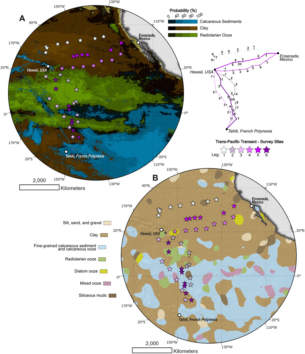
Figure 1. Predictive maps of seafloor sediment cover for the a region of the Pacific Ocean that encompasses the Trans Pacific Transit. (A) Predictive model produced by Diesing (2020). (B) Predictive model produced by Dutkiewicz et al. (2015).

Work by Diesing (2020) has produced a far simpler global seafloor composition map based upon the five dominant lithology classes (Figure 1). This map is more resemblant of earlier work (Bershad and Weiss, 1976; Trujillo and Thurman, 2014) and shows a stark contrast to the complex patchwork of sediment distribution generated by Dutkiewicz et al. (2015). Utilising a combination of the seafloor sample database (Dutkiewicz et al., 2015) and a suite of environmental predictors (Tyberghein et al., 2012; Sbrocco and Barber, 2013; Assis et al., 2018), the predictive map indicates a dominance of clay and calcareous sediments throughout most of the global oceans between ∼50° N and 50° S (Diesing, 2020), which is comparable to results identified by Dutkiewicz et al. (2015), Dutkiewicz et al. (2016). The Pacific Ocean is split with a dominance of clay in the northern regions and calcareous sediments dominating the majority of the southern Pacific Ocean. However, the equatorial and tropical regions of the Pacific are dominated by an extensive belt of radiolarian sediments, similar to previous global seafloor sediment maps (e.g., Bershad and Weiss, 1976; Trujillo and Thurman, 2014). However, these predictions still require validation, as confidence levels in the sediment types vary considerably, primarily due to the variability of the spatial density of sediment samples. Furthermore, less dominant sediment types (i.e., diatom ooze, lithified sediments and radiolarian ooze) may be less represented by environmental predictors, thus impacting the accuracy of the seafloor sediment maps (Diesing, 2020).

Alongside the composition of the superficial sediments of the seafloor, abyssal plains in all major oceans can be characterised by the presence of polymetallic nodules that are usually identified on top or just below the surficial sediment layer (Menard, 1964; Hein et al., 2013; Hein et al., 2020; Hein and Koschinsky, 2014; Hein, 2016; Kuhn et al., 2017; Kuhn and Rühlemann, 2021). Polymetallic nodules, comprising concentric layers around a nucleus, are known from the sediment-covered abyssal depths of the Pacific Ocean, such as the Clarion–Clipperton Fracture Zones, and form either through precipitation from seawater or pore waters within deep-sea sediments although are commonly a mix of both genetic types (Menard, 1964; Kuhn et al., 2017; Hein et al., 2020). The nodules and the soft sediment around them create a complex and distinct habitat that hosts highly diverse communities in the abyss (Vanreusel et al., 2016; Schoening et al., 2020; Uhlenkott et al., 2023; Niyazi et al., 2024).

The majority of the work on nodule occurrence and distribution has focused on the abyssal plains of the Pacific Ocean. However, this has resulted in a lack of understanding of worldwide occurrence (Dutkiewicz et al., 2020), and even within the Pacific Ocean, nodule identification is predominately focused in zones considered for deep sea mining exploration (Hein et al., 2013; 2020; Lodge et al., 2014; Wedding et al., 2015; Liu et al., 2024). The prediction of nodule occurrence has become increasingly important with the regulation and identification of deep-sea mining locations and more importantly for quantifying the ecosystem function and ecological habitat of nodule fields (Vanreusel et al., 2016; Simon-Lledó et al., 2019; Dutkiewicz et al., 2020; Stratmann et al., 2021; Uhlenkott et al., 2023).

This study aims to: (i) determine the composition and coverage of seafloor sediment on the abyssal plains in the central and eastern Pacific Ocean; (ii) test machine learning derived spatial models of seafloor sediment composition; and (iii) discuss the occurrence and distribution of polymetallic nodules. We utilise remotely-sensed lander-derived observations of the seafloor and spatially concurrent oceanographic and geological datasets to achieve these aims.

Methods

The Trans-Pacific Transit (TPT) Expedition, a six-leg transit of the Pacific Ocean onboard R/V Dagon (Figure 2), has provided remote imagery and video footage of seafloor sediments and habitats of the central and eastern Pacific Ocean (Jamieson et al., 2024). The TPT Expedition traversed 20,667 nautical miles between start/end points of Ensenada (Mexico), Hawaii (USA) and Tahiti (French Polynesia). Scientific landers were deployed 123 times across 43 survey sites, at depths ranging between 3,600 and 6,800 m (Figure 2; Supplementary Table SB1), acquiring 900+ hours of video footage of the abyssal seafloor environment (Jamieson et al., 2024).

Figure 2

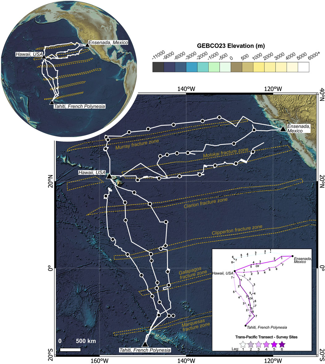
Figure 2. Location of the Trans-Pacific Transit (TPT) within the Pacific Ocean. White lines show ship track for the Trans Pacific Transit and black points indicate the lander deployment sites. Yellow dotted lines indicate the boundary of Pacific Ocean fracture zones (Hartwell et al., 2018). The inset map shows the individual legs of the Trans Pacific Transit expedition and their related lander deployment sites.

Free-fall scientific landers

A fleet of four autonomous free-fall landers were used (named Omma, Magna, Cranch and Chiro) to obtain video footage and oceanographic data (Supplementary Table SB1). Landers were deployed 2 km apart in a triangle shape at each of the 43 sites, locations where the seafloor slope angle was <4° were preferentially selected. See supplementary B for detailed specifications and payload of each lander system deployed during the TPT.

Analysis of lander footage

A selection of three 5-minute clips were extracted from the video footage collected at each site where available. This included a clip of the lander touching down on the seafloor, a clip midway through the observation period and a clip at the end of the observation as the ballast weight was released. Video data were analysed to assess the sediment colour, grain size, presence of polymetallic nodules and bedrock exposure, and any other interesting characteristics (e.g., xenophyophores, surficial burrows, etc.). For example, distinctive variations in sediment colour can be used effectively to identify between clay (i.e., pale brown, brown, orangey-brown) and calcareous sediments (white, off-white, yellowish-white). Furthermore, qualitative assessment of grain size (fine-grained vs. coarse-grained) can be used to identify the presence of either clay/biogenic sediments (fine) or lithified sediments (coarse). Seafloor features with a large enough size were possible to measure quantitatively with the aid of laser scales attached to the landers. An interpretation of the sediment type was made based on what was observed in lander footage and validation based upon comparison against the sediment type from the nearest sample locations (Supplementary Table SC1) and predictive seafloor maps. A qualitative assessment of polymetallic nodule density within the field of view was undertaken if nodules were present (Supplementary Figure SB1).

Multibeam-derived parameters

R/V Dagon is equipped with a full-ocean depth, hull-mounted Kongsberg EM 124 multibeam echosounder (MBES) system for collecting bathymetric and backscatter intensity data. Bathymetric data were processed by manual editing and automatic spike filtering techniques in QPS processing software Qimera (version 2.5). A Digital Bathymetric Model (DBM) with the cell size of 100 m was generated and uploaded to GIS software for further analysis. For additional information of the bathymetry system, alongside collection and processing workflows, see Jamieson et al. (2024). Derivatives, such as TRI (Terrain Ruggedness Index) and slope were calculated using in ESRI ArcGIS Pro (version 3.2) using Raster Functions and Spatial Analyst extension, and were used to provide additional geomorphological context to the interpretation of the seafloor substrate. An automated classification of the DBM using the Geomorphons tool (Jasiewicz and Stepinski, 2013) was also undertaken in ESRI ArcGIS Pro using the Spatial Analyst extension. Geomorphons were calculated on the filled and filtered DBM with a 20 × 20 pixel search window (equivalent to 2 × 2 km) and a flat terrain threshold of ≤3°. Values were extracted to understand the morphological characteristics within a buffer radius of 0.5 km around each lander site location. Topographic derivatives are included within the compiled dataset (see Supplementary data) but were mostly excluded from further analysis due to sampling bias associated to the preferential selection of lander deployment locations.

Supporting datasets

In order to improve the validation of the video-derived sediment, bedrock and polymetallic nodule analysis, a number of supporting geological and oceanographic datasets were collated, which include: predictive surficial sediment maps; sediment thickness; seafloor age; average sedimentation rate; nodule probability; sea surface temperature; chlorophyll; modelled particulate organic carbon (POC); dissolved oxygen; dissolved inorganic nutrients (nitrate, phosphate and silicate); interpolated bottom oxygen measurements; and simulated bottom current speed fluctuation (expressed as standard deviation).

Predictive seafloor surficial sediment maps were acquired from Dutkiewicz et al. (2015) and Diesing (2020) and have a gridded resolution of 0.1-arc-degree and 10 × 10 km, respectively. Information of the sediment type was extracted from each predictive grid to compare and validate with analysis from lander-derived seafloor footage (see Supplementary data). This was further supplemented with information of seafloor sediment composition gained from the nearest sediment core to each lander deployment, acquired from the Curators of Marine and Lacustrine Geological Samples Consortium (2024) database (see Supplementary data). Sediment core data was utilised to validate interpretations of sediment cover from lander footage. This was accomplished by identifying sediment type reported in the core and evaluating its confidence to reliably validate the lander footage as a result of the proximity to the lander deployment location (see Supplementary Table SC2).

Information of seafloor sediment thickness was extracted from the GlobSed global 5-arc-minute surface (Straume et al., 2019). The seafloor age was extracted from a global age model gridded at a 2-arc-minute resolution (Seton et al., 2020). Average sedimentation rate (Dutkiewicz et al., 2017) and polymetallic nodule probability data were acquired from 0.1-arc-degree resolution surfaces that were accessed through the supplementary data within Dutkiewicz et al. (2020). Annual average values for sea surface temperature, Chlorophyll-a, and POC were obtained from the MODIS satellite database (Ocean Biology Processing Group, 2023). These values were calculated as annual averages from 2002 to 2022 for each lander deployment, considering radii of 20, 40, and 80 km. The variation between different radii was minimal for all three parameters (Supplementary Figures SB3–SB5), so only the 20 km radius values were used in the analysis. Interpolated combined measured datasets of surface salinity (Reagan et al., 2024b), dissolved oxygen (Garcia et al., 2024b) and dissolved inorganic nutrients (Garcia et al., 2024a) were downloaded from the World Ocean Atlas (Reagan et al., 2024a) and sampled at 1-arc-degree grid resolution of the average value for all available years (i.e. 1955 – 2022). Bottom oxygen data (Seiter et al., 2005) and bottom current data (Thran et al., 2018) were sampled at 0.1-arc-degree grid resolution and accessed through the supplementary data within Dutkiewicz et al. (2020).

All supporting datasets were imported into ArcGIS Pro and projected in the WGS 84 coordinate system prior to the extraction of data values to a shapefile containing the location of each successful lander deployment. Analysis was then performed to identify relationships between seafloor sediment composition, the presence of nodules, and related geological and oceanographic conditions.

Results

Seafloor sediment cover

Overlaying lander deployment locations on predictive deep sea sediment maps provided an insight into the likely surficial sediments that could be identified in lander footage (Figure 2). Predictive maps produced by Diesing, (2020) (Figure 2A) and Dutkiewicz et al. (2015) (Figure 2B) mostly agree on a dominance of clay for Legs 1, 4 and 5. The probability of the surficial sediment being clay for Leg 1, 4 and 5 ranges between 0.4 and 0.8 (Supplementary Figure SC1; Diesing, 2020).

Analysis of video footage from the lander deployments indicates three generalised surficial sediments; calcareous sediments, clays, and radiolarian sediments (Figures 3, 4). Interpretation of video footage indicates clay is the dominant seafloor substrate (e.g., 80 out of 124 lander locations, Figure 4). Seafloor sediments identified as clay are predominantly present in footage captured in Legs 1, 4 and 5 (20–35° N), where it was interpreted in 100% of the lander deployments (Figure 4). However, at lander sites visited during transits between Hawaii and Tahiti (i.e., legs 2, 3 and 6) this varies considerably with the inclusion of radiolarian (13.8% of all lander locations) and calcareous (20.3% of all lander locations) dominated sediments (Figure 4). The spatial distribution of these sediments generally agrees with predictive maps of seafloor lithology (Dutkiewicz et al., 2015; Diesing, 2020) and the closest collected sediment samples (e.g., Curators of Marine and Lacustrine Geological Samples Consortium, 2024) to the lander locations (Supplementary Table SC1). However, the predictive lithology produced by (Diesing, 2020) misinterprets calcareous sediments as radiolarian sediments in multiple instances (e.g., Figure 1). One lander location is interpreted as lithified due to the field of view being completely dominated by a pavement of cemented polymetallic nodules, thus making the interpretation of surficial sediments untenable.

Figure 3

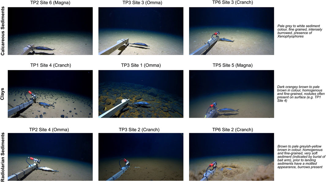
Figure 3. Screenshots of seafloor sediment coverage captured during the trans pacific transit lander deployments. See Figures 1, 2 for lander site locations.

Figure 4

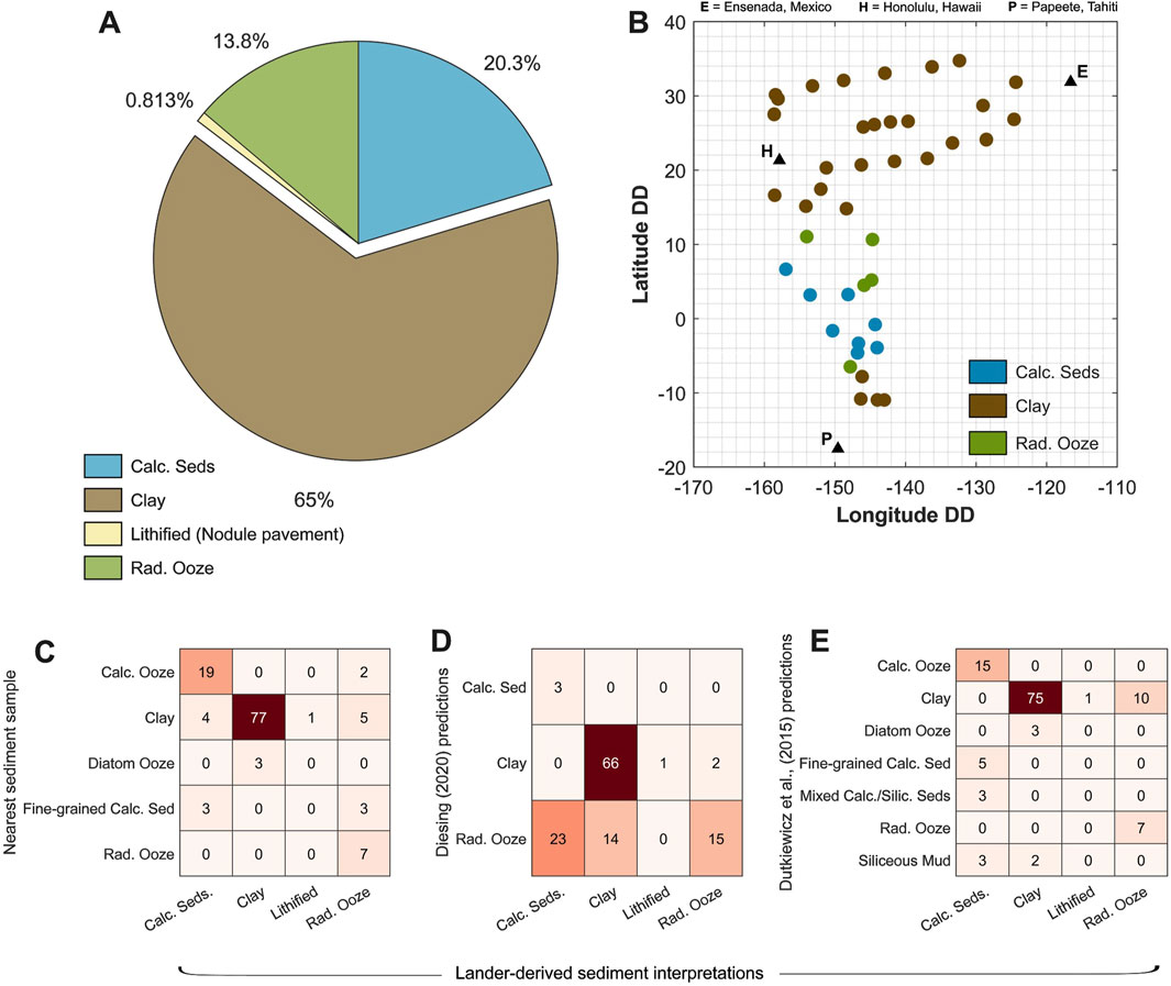
Figure 4. (A) Percentage of different sediment types identified during the Trans Pacific Transit. (B) Geographic distribution of sediment types (C–E) Heatmaps showing similarities or differences in observed sediment composition between lander-derived interpretations and other seafloor composition datasets (Dutkiewicz et al., 2015; Diesing, 2020; Curators of Marine and Lacustrine Geological Samples Consortium, 2024; Dutkiewicz et al., 2015; Diesing, 2020; Curators of Marine and Lacustrine Geological Samples Consortium, 2024).

Sediments interpreted as calcareous are viewed in the lander footage as pale grey to white in colour and fine-grained (Figure 3). In the majority of video footage where calcareous sediment is classified, the seafloor is characterised by extensive burrowing, lebensspuren and the presence of xenophyophores within the field of view (Figure 5). Calcareous sediments were identified at a latitude range of 4.6° S to 6.7° N and where water depths ranged between 4465–4937 m (Figure 6). Calcareous sediments were identified where average sea surface temperatures are high (26.4–28.4°C), surface oxygen is low (198.8–201.5 mmol m⁻³), and surface productivity (e.g., Chlorophyll-a) and nutrients (Nitrate, Phosphate and Silicate) are high (Figure 6; Table 1; Supplementary Table SC2). Calcareous sediments are also located where there is an increased sediment thickness (283.03 m average) and sedimentation rate (0.46 cm ka⁻¹ average).

Figure 5

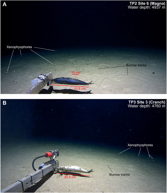
Figure 5. Example of calcareous sediment identified from lander footage. (A) TP2 Site 6 – 4937 m water depth. (B) TP3 Site 3 – 4760 m water depth. See Figures 1, 2 for lander site locations.

Figure 6

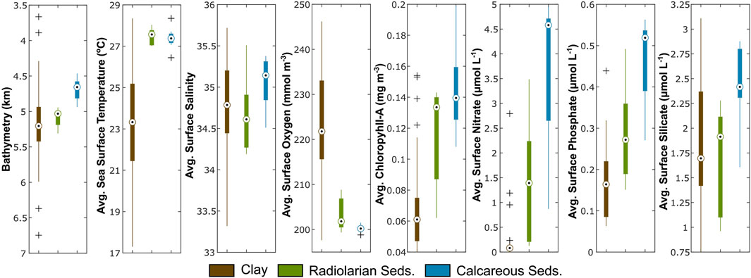
Figure 6. Boxplots of the values of key oceanic parameters at interpreted seafloor sediment locations. See Supplementary Tables SC3, SC4 for statistical comparisons of the oceanic variables.

Table 1

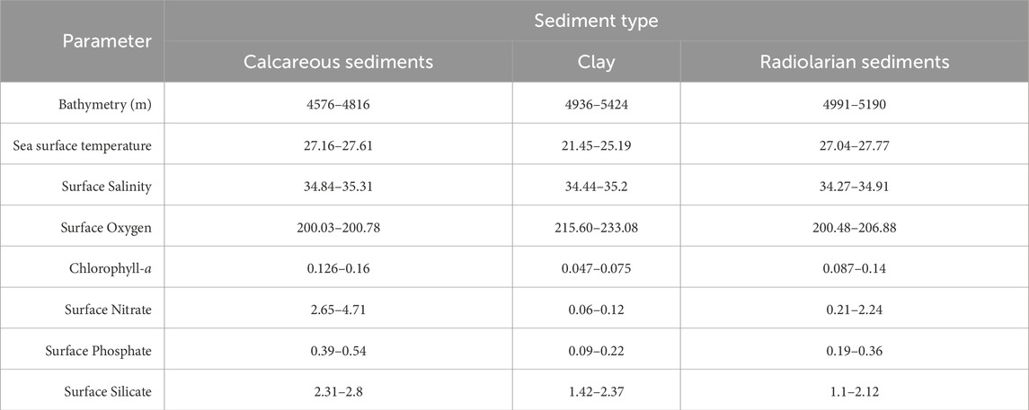
Table 1. Interquartile ranges of key oceanic parameters (Figure 6) for identified surficial seafloor sediments. See Supplementary Tables SC3, SC4 for statistical comparisons of the oceanic variables.

Clay is variable in colour from a pale greyish-brown to a dark orangey-brown (Figure 3). The clay always appears fine-grained with a homogenous coverage in the lander imagery. Sites comprising polymetallic nodules and exposed bedrock are often coincident with clay substrate, either present as a veneer or matrix on the seafloor. Identification of clay spans lander deployments that cover the entire range of water depths (i.e. 3664 – 6746 m), average sea surface temperature (17.3–28.3°C) and bottom temperature (1.4–1.7°C), average surface salinity (33.32–35.72 PSS) and bottom salinity (34.68–34.71 PSS), average surface oxygen (197.6–246.2 mmol m⁻³) and bottom oxygen (133.3–187.49 mmol m^-3), and average surface silicate (0.76–3.1 μmol L⁻¹), across the entire survey (Figure 6; Supplementary Table S2). Where clay is observed at the seafloor, the surface productivity (deduced through average Chlorophyll-a), and surface nutrients (e.g., Nitrate and Phosphate) are reduced compared to other key oceanic parameters (Figure 6; Table 1). Furthermore, there is a statistically significant difference in the average value of these parameters (i.e., surface productivity and nutrients) where the seafloor sediments are interpreted as clay compared to those for the calcareous and radiolarian sediments (Supplementary Tables SC3 and SC4).

Radiolarian sediments were the most difficult to interpret due to limited variations in colour or homogeneity of the sediment cover whilst the lander was stationary on the seafloor. However, the identification of radiolarian sediments became apparent due to a variation of the seafloor surface cover before the lander reached the seafloor and once it left (Figure 7). The sediment cover had a characteristic mottled pattern with colours varying between light grey and an orangey/reddish brown prior to the lander settling on the seafloor (Figure 7). Once the lander settled on the seafloor, the sediments appeared to be a pale greying brown and very soft, indicated by the partial burial of the bait arm (Figure 7B). There is a moderate level of confidence with the interpretation of radiolarian sediments as their observation in the lander footage is coincident, and constrained by high probabilities of radiolarian sediments at the lander sites (Figure 1; Supplementary Figure SC1) combined with samples/cores of radiolarian dominated sediments that were in close proximity to the lander location (Supplementary Table SC1). Radiolarian sediments are identified where average sea surface temperatures are at the highest levels (27–28°C) for lander sites and comparable to the temperature where calcareous sediments are observed (Figure 6). Furthermore, sites with radiolarian sediments had the lowest levels of average surface oxygen and these were statistically different from sites with clay but not sites with calcareous sediments (Figure 6). Surface productivity and nutrient concentrations at lander sites characterised by radiolarian sediments sit within a mid-range between the relatively lower values at sites where clay is present, and the higher values where the seafloor is characterised by calcareous sediments (Figure 6).

Figure 7

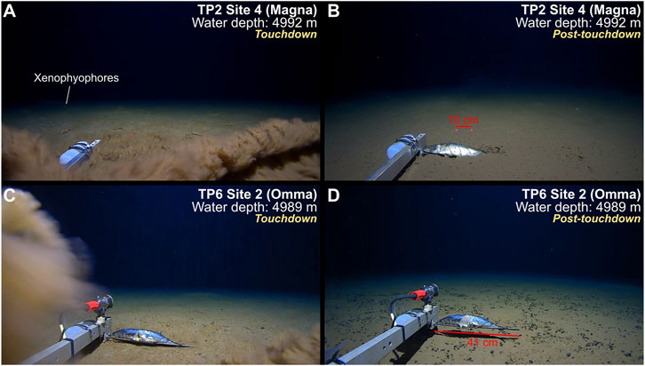
Figure 7. Example of interpreted radiolarian sediment identified from lander footage. (A) TP2 Site 4 (touchdown) – 4992 m water depth. (B) TP2 Site 4 (post-touchdown) – 4992 m water depth. (C) TP6 Site 2 (touchdown) – 4989 m water depth. (D) TP6 Site 2 (post-touchdown) – 4989 m water depth. See Figures 1, 2 for lander site locations.

A number of interesting relationships have also been identified where there are observations of key oceanic parameters (i.e., temperature, salinity and oxygen) both at the surface and on the seafloor. Calcareous and radiolarian sediments generally show a preferential clustering compared to clay when comparing temperature, oxygen and salinity (e.g., Figure 8). Negative linear relationships exist when comparing surface and bottom temperature, bottom salinity and bottom temperature, and bottom and surface oxygen concentrations (Figures 8A, E, F). Both radiolarian and calcareous sediments are clustered in locations where surface temperatures are high (26.4–28.4°C) and bottom temperatures are low (1.35–1.48°C) and show a statistically significant variation from clay (Figure 8A; Supplementary Tables SC3, SC4). However, it is worth noting the increased sample size of the clay observations compared to other observed seafloor sediment compositions (e.g., Figure 4A). Calcareous and radiolarian sediments are present in locations where the bottom oxygen is relatively high (170–190 mmol m^-3) and surface oxygen is relatively low (200–210 mmol m^-3), which is significantly different compared to oxygen concentrations where clay is found (Figure 8F; Supplementary Tables SC3, SC4). Similarly, there is clustering of deployments with calcareous sediments at both higher surface (34.5–35.4; Figure 8) and seafloor salinity (34.69–34.71) and shows a significant variation when compared to clay and radiolarian sediments (Supplementary Tables SC3, SC4). There is a strong positive linear relationship between Chlorophyll-a and POC (which is expected as POC is calculated from Chlorophyll-a), with calcareous sediments present at relatively high concentrations (median Chla: 0.14 and median POC: 49.89, Figure 9; Supplementary Tables SC2 – SC4). Radiolarian sediments also appear to present with higher concentrations of Chlorophyll-a and POC, but this relationship is less pronounced (median Chla: 0.13 and median POC: 48.27, Figure 9; Supplementary Tables SC2 – SC4). Concentrations of Chlorophyll-a and POC at the surface are generally low where clay is present on the seafloor, median values of 0.08 and 30.68, respectively.

Figure 8

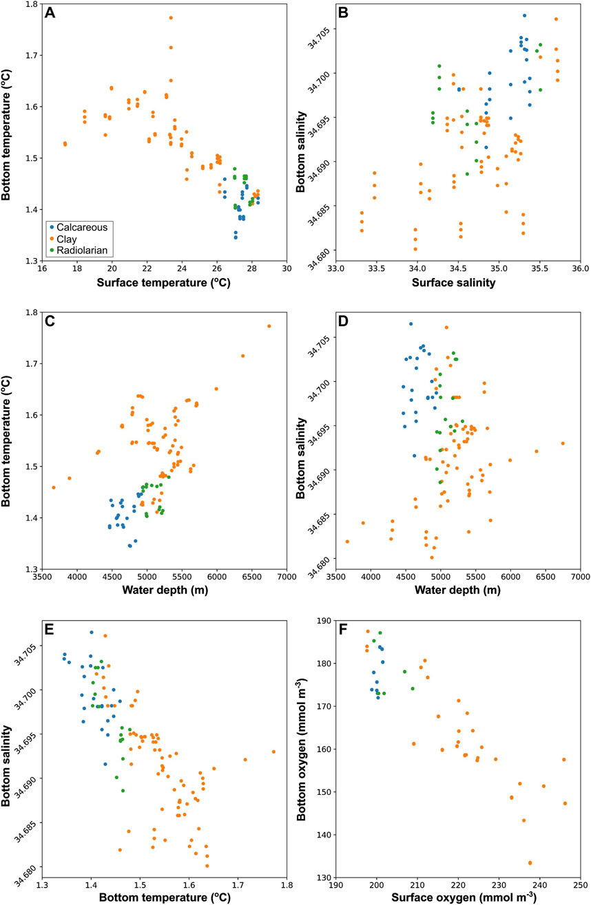
Figure 8. Scatterplots of sediment type and selected oceanographic variables (A). Bottom temperature vs. surface temperature (B). Bottom salinity vs. surface salinity (C). Bottom temperature vs. water depth (D). Bottom salinity vs. water depth (E). Bottom salinity vs. bottom temperature (F). Bottom oxygen vs. surface oxygen.

Figure 9

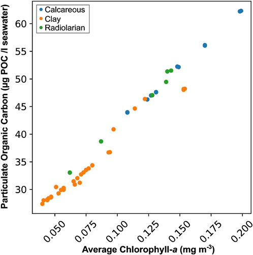
Figure 9. Scatterplot showing the link between average Chlorophyll-a, POC and sediment type for lander deployments across the TPT.

Polymetallic nodule distribution

Analysis of all available lander footage revealed the presence of nodules in 55% of lander deployments (Figure 10). Most lander sites and deployments with a positive identification of nodules were located between 20° – 35° N (Figure 10B). Nodule sizes generally range between 2–5 cm (utilising laser scale and the lander bait arms for scale, e.g., Figure 11) but in some locations are up to 10–15 cm in length (e.g., TP2_OM3_5400 in Figure 11C). Where nodules are present, the average nodule probability (Dutkiewicz et al., 2020) ranges between 0.15 and 0.79 with an average of ∼0.48 (Figure 10B). Nodule identification predominately occurred at lander sites where the seafloor sediment cover was interpreted as clay (83% of positive nodule identifications). Approximately 18% (12 out of the 68 lander deployments with nodules) of the lander deployments with nodules present (6 out of a total of 42 lander sites visited) are located within fracture zones (Murray, Molokai, Clarion and Galapagos) (Figure 10). Furthermore, 31% of deployments that observed nodules are within 100 km of a fracture zone and 60% are within 200 km. Roughly 28% of lander deployments with nodules in the footage are associated with the presence of dense nodule fields (>70% coverage within field of view of lander imagery) (Figure 11). Of those dense nodule fields, 68% lie within 200 km of fracture zones (Murray and Molokai) and are predominately located between 20–35° N latitude (Figure 11) where the surficial sediment cover is interpreted as clay (e.g., Figure 4). Additionally there is reduction in values associated to Chlorophyll-a, sediment thickness and sedimentation rate (Figure 12). The cluster of lander deployments from Leg 2, 3 and 6 between latitudes of 4° S and 6° N that do not record the presence of nodules in the lander footage are coincident with a zone of increased sediment thickness, sedimentation rates and Chlorophyll-a (Figure 12). Low rates of sedimentation and sea surface productivity are important for nodule formation or preservation on the surface of the seafloor (e.g., Dutkiewicz et al., 2020). Sedimentation rate is suggested to be the most important of these factors (e.g., Dutkiewicz et al., 2020), however, it is likely that a greater influence on nodule formation occurs when multiple parameters are spatially coincident (e.g., Figure 13).

Figure 10

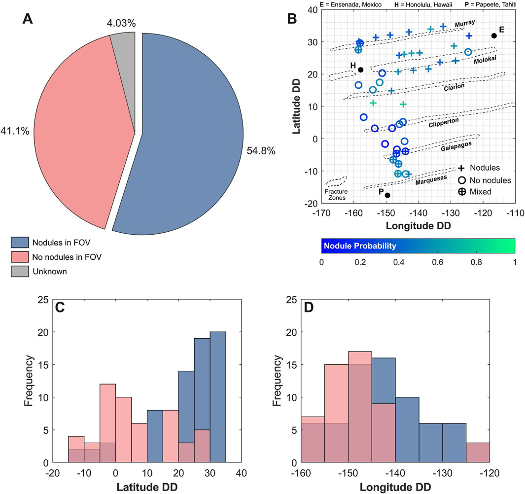
Figure 10. (A). Percentage of Trans Pacific Transit lander deployments with nodule observations. (B). Geographic distribution of nodule occurrence across the Trans Pacific Transit. Nodule probability acquired from Dutkiewicz et al. (2020). (C, D). Histograms of nodule occurrence over latitude and longitude.

Figure 11

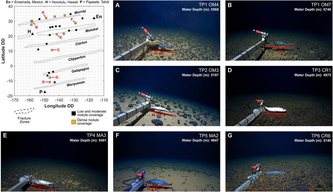
Figure 11. Screengrabs of dense nodule fields observed within the lander footage from the Trans Pacific Transit dataset. (A) TP1 Site 4 – 5568 m water depth. (B) TP1 Site 7 – 6746 m water depth. (C) TP2 Site 3 – 5197 m water depth. (D) TP3 Site 1 – 4875 m water depth. (E) TP4 Site 3 – 5491 m water depth. (F) TP5 Site 2 – 4647 m water depth. (G) TP6 Site 6 – 5140 m water depth. See Figures 1, 2 for lander site locations.

Figure 12

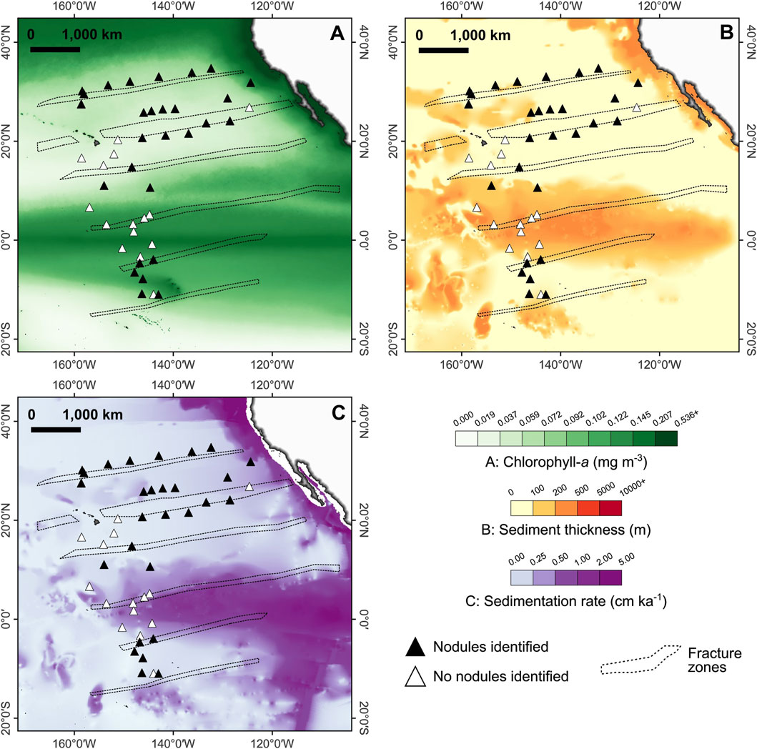
Figure 12. Nodule occurrences and their spatial coincidence with average annual (2002–2022) Chlorophyll-a (A), sediment thickness (B) and sedimentation rate (C).

Figure 13

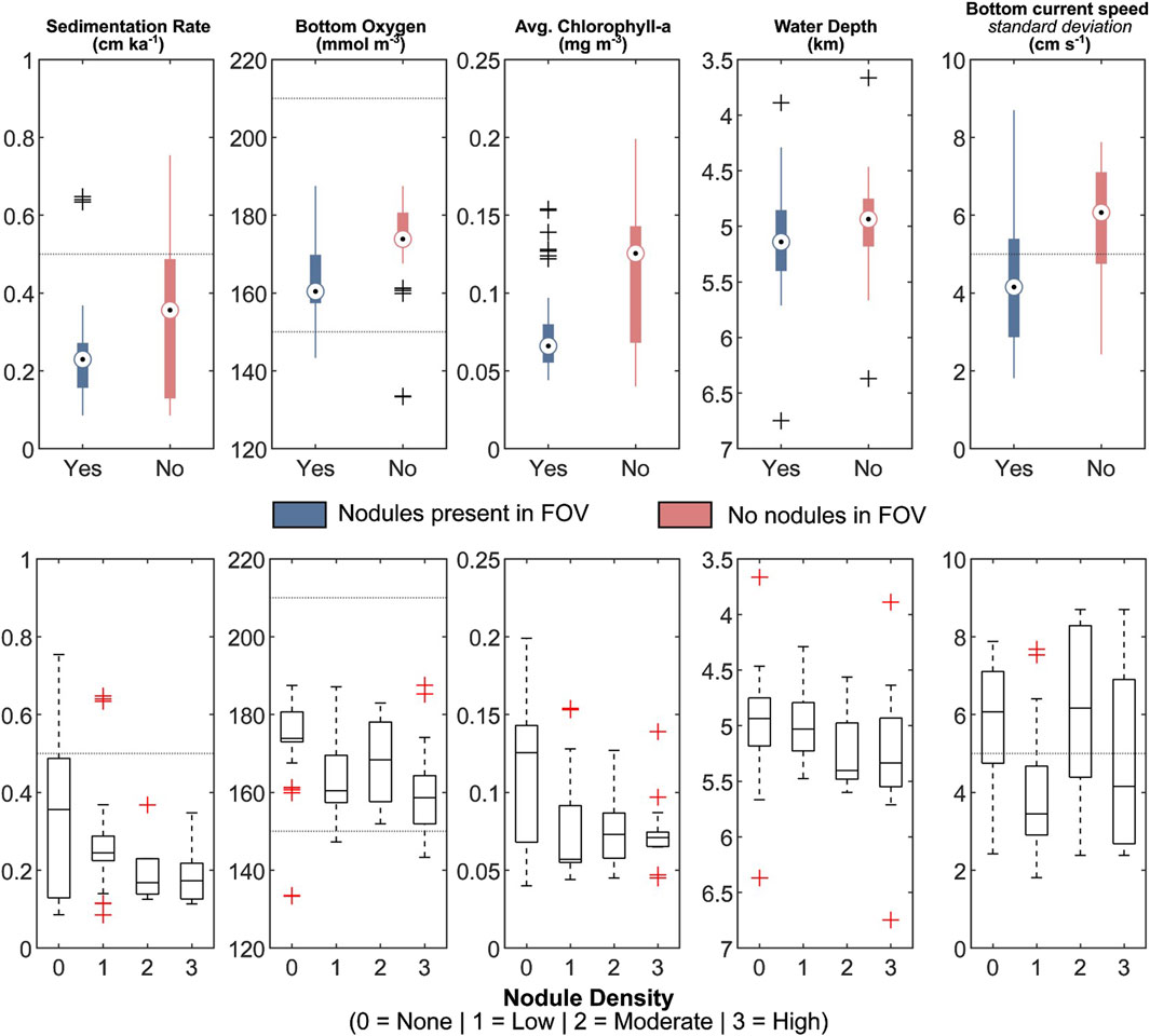
Figure 13. Boxplots of the values of key oceanic parameters for nodule formation (e.g., Dutkiewicz et al., 2020) for positive and negative nodule identifications in lander deployments for the Trans Pacific Transit.

Discussion

Results from this study support the consensus that clay and calcareous sediments are the most dominant lithologies of seafloor sediments in the Pacific Ocean abyssal plains (Menard, 1964; Berger, 1974; Berger, 1976; Bershad and Weiss, 1976; Davies and Gorsline, 1976; Barron and Whitman, 1981; Bickert, 2009; Hüneke and Mulder, 2011; Trujillo and Thurman, 2014; Dutkiewicz et al., 2015; Dutkiewicz et al., 2016; Diesing, 2020). Clay is particularly dominant in the northern latitudes of the study area and is mostly seen in lander deployments during the transits between Ensenada and Hawaii (Legs 1, 4 and 5, Figures 1, 4). Deep sea red clays are well known to be a residual sediment product formed by the dissolution of biogenic components (Berger and Winterer, 1974). However, especially within the Pacific Ocean, the majority of the deep-sea clay located distal of land masses (100s–1000s of km’s away) is detrital and has sedimentological compositions (e.g., abundances of chlorite, illite, etc.) that suggest deposition through aeolian processes (Fagel, 2007; Lisitzin, 2011; Dutkiewicz et al., 2016). It has previously been estimated that deposition of material through aeolian processes into the global oceans is comparable to the total fluvial input of sediment (Lisitzin, 2011). The average depth for the landers deployed in Legs 1, 4 and 5 is 5164 m WD which corresponds to the understanding that clay lithologies dominate the seafloor in locations below 4500 m WD (Zeebe, 2012; Dutkiewicz et al., 2016). Clay can be found at shallower depths but requires regions that generally have low levels of surface productivity and low levels of surface salinity (i.e., <33 PSS), such as continental margins (Dutkiewicz et al., 2016). Furthermore, clay sediments are located where surface productivity is significantly reduced (Figure 6) which enables their preservation because of reduced production and sedimentation rate of biogenic oozes (e.g., calcareous and silicious sediments). Clay can occur in zones of high surface productivity but relies on the seafloor being below 4500 m WD (average CCD limit) and the plankton population being dominated by calcareous organisms and not siliceous organisms (Dutkiewicz et al., 2016).

Calcareous sediments in the central and eastern pacific ocean

The identification of calcareous sediments to depths exceeding 4900 m (e.g., Figures 5, 6) is one of the most intriguing results from the sedimentological analysis of the lander footage. Calcareous sediments in the Pacific Ocean are believed to predominately occur shallower than 4500 m WD, because of the CCD limit varying between ∼4000–4800 m WD across different regions of the ocean (Berger et al., 1976; Zeebe, 2012; Sulpis et al., 2018; Simon-Lledó et al., 2023) (Table 2). Of the lander deployments in which we identify calcareous sediments, 88% (22 out of 25) are below the suggested average (4500 m WD) CCD limit (Pälike et al., 2012; Zeebe, 2012) for the Pacific Ocean and 100% are below the CCD limit reported for the central equatorial pacific region (e.g., Table 2; Sulpis et al., 2018). We therefore propose a maximum CCD limit for the equatorial pacific region of 5000 m WD. The identification of calcareous sediments up to 5000 m WD is reported in the North Atlantic Ocean, and is the dominant seafloor sediment type, which is largely attributed to the presence of the CCD limit at ∼5100 m WD (Broecker, 2008; Dutkiewicz et al., 2016). The identification of the calcareous sediments up to 5000 m WD in the equatorial and tropical zone of the southern Pacific Ocean is most likely attributed to the influence of the Pacific equatorial upwelling zone (Lyle et al., 2008; Pälike et al., 2012; Zhang et al., 2017) and high productivity of the eastern Pacific influencing the CCD (Berger and Winterer, 1974). The increase of net primary production of planktonic carbonate shells in the equatorial upwelling zone can depress the CCD by ∼500 m (Johnson et al., 1977; Bickert, 2009), which is similar to the variation we observe (e.g., Figure 6). All locations of calcareous sediments identified in this study are coincident with regions of higher productivity (e.g., increased levels of average Chlorophyll-a), however the spatial pervasiveness of the effect of the equatorial upwelling and increased production on CCD is unknown. Suggestions of enhanced CaCO₃ burial linked to glacial inception in Antarctica have also been suggested for the overdeepening of the CCD within equatorial regions of the Pacific Ocean (Archer, 1996; Taylor et al., 2023).

Table 2

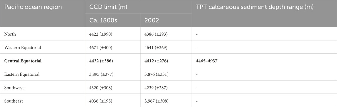
Table 2. Carbonate compensation depth (CCD) limits within regions of the Pacific Ocean acquired from (Sulpis et al., 2018). Row highlighted in bold to indicate comparison between previously reported CCD limits for the central equatorial region of the Pacific Ocean and our coincident observations of calcareous sediments.

Calcareous sediments are observed where the bottom oxygen values are relatively high and bottom temperatures are relatively low to all other lander sites (Figure 8). This increased oxygen level in the equatorial regions of the pacific is likely a factor in the deeper limit of the CCD and thus presence of calcareous sediments at the seafloor (Sulpis et al., 2018; Harris et al., 2023). Bottom oxygen concentration decreases into the north-east Pacific due to a lack of deep-water formation, and mixing of bottom waters with the overlying water masses (Talley, 2007; Talley, 2013). Thus, influencing a shoaling of the CCD limit (Sulpis et al., 2018; Simon-Lledó et al., 2023). Bottom water controlled variability in oxygen levels at depth may influence the depth of the CCD as the CO₂ concentrations will vary accordingly. For example, enhanced CO₂ concentrations within ocean masses can lead to the CCD limit rising to shallower water depths (Sulpis et al., 2018; Harris et al., 2023; Simon-Lledó et al., 2023). Increased understanding of the spatial variation in limits of the CCD across the oceans is critical in order to quantify any changes as a result of climate-driven increases in oceanic CO₂ levels (Sulpis et al., 2018; Harris et al., 2023; Simon-Lledó et al., 2023). Furthermore, greater comprehension of the present-day variability of the CCD in the global ocean is a crucial step to enhance the ability to accurately predict the seafloor sediment type, which in turn has important implications for the distribution of marine life and palaeoceanographic reconstructions.

Radiolarian sediments in the central and eastern pacific ocean

Radiolarian ooze is likely to be more sporadic in the Pacific Ocean abyssal plains compared to what is predicted by Diesing, (2020) and reported in previous studies (Menard, 1964; Berger, 1974; Berger, 1976; Davies and Gorsline, 1976; Barron and Whitman, 1981; Hüneke and Mulder, 2011; Trujillo and Thurman, 2014). The results presented here are comparable to the predictive map of Dutkiewicz et al. (2015). However, it is important to note that it is difficult to confidently identify radiolarian ooze from the lander footage, especially without a coincident sediment sampling regime. Though it was possible to distinguish where calcareous sediments were present rather than the radiolarian predicted by Diesing, (2020) (e.g., Figures 3, 4). We observe 23 sites characterised by calcareous sediments in the lander footage where radiolarian ooze was believed to be present (e.g., Figure 4D; Diesing, 2020). As previously discussed, this is likely a result of model forcing increasing the importance of bathymetry linked to the limit of the CCD. Radiolarian ooze is more likely to have a spatially sporadic sediment cover that occurs in localised regions where specific oceanographic conditions are met. Therefore, contradicting the predictive model proposed by Diesing, (2020) where radiolarian ooze is identified as the third most dominant seafloor lithology (∼14% of the global ocean seafloor coverage), instead it is likely to be of the most rare surficial sediment covers.

Radiolarian ooze has two discrete communities that differ in spatial location (e.g., equatorial regions of the Pacific and Indian oceans, and the Southern Ocean) and controlling oceanographic variables. Within the equatorial region of the Pacific Ocean, radiolarian ooze formation is believed to be a product of a sea surface temperature range between 25–30°C, surface salinity range of 33–35 PSS, and surface productivity that is relatively low compared with where calcareous sediment is present on the seafloor (Dutkiewicz et al., 2016). However, it has also been suggested that radiolarian ooze occurs where surface productivity is high (De Wever and Baudin, 1996; De Wever et al., 2001). Where we interpret radiolarian ooze, there is general agreement with the range of controlling variables suggested by Dutkiewicz et al. (2016) (e.g., Figure 6). Furthermore, surface productivity (i.e., Avg. Chlorophyll-a) is significantly lower at locations where radiolarian sediments are recorded compared to those dominated by calcareous sediments (e.g., Figure 6; Supplementary Tables SC3, SC4). This suggests that radiolarian ooze can be preferentially present on the seafloor surface at the fringes of higher productive regions. Where surface productivity is at its highest, however, it is likely that radiolarian sediments are masked by dominant sedimentation of calcareous sediments, especially where the CCD is lowered as a result of equatorial upwelling (Peterson and Prell, 1985; Bickert, 2009).

Polymetallic nodule distribution within the central and eastern pacific ocean

Most of the positive polymetallic nodule identifications within the study area are at locations considered unlikely for nodule formation/preservation (average probability of 0.48), suggesting predictive models (e.g., Dutkiewicz et al., 2020) of nodule distribution still require further development. However, to allow for the improvement of predictive models, an increase in the understanding of the spatial distribution of nodule fields through the provision of ground-truth datasets in the global ocean is required, as opposed to a focus solely on deep-sea mining exploration locations (Hein et al., 2013; Hein et al., 2020; Lodge et al., 2014; Wedding et al., 2015). Polymetallic nodules are present in video footage of more than half of the lander deployments, indicating their commonality as a seafloor feature in the Pacific Ocean, particularly in the north-central (10–40° N) and eastern (120–160° W), and clay-dominated regions of the Pacific Ocean.

The abundance of nodules on clay-dominated substrates is to be expected due to the lower rates of sedimentation associated with seafloors composed of pelagic clay (e.g., Figures 12C, 13). Nodule formation is known to be controlled by long-term sedimentation at low rates usually <0.5 cm ka⁻¹. The majority (96%) of positive nodule identifications within this study are below this 0.5 cm ka⁻¹ sedimentation rate threshold value. Lander deployments in areas above the 0.5 cm ka⁻¹ threshold are all located at the same site (e.g., TPT Leg 5 Site 1) and are considered nodule fields that have a low density coverage. Furthermore, the sedimentation rate at TPT Leg 5 Site 1 (i.e. 0.63 cm ka⁻¹, Figures 2, 13) is only marginally above the threshold value. Nodule formation occurs more favourably in regions of low sedimentation as it allows significant exposure time for nodule growth and development (von Stackelberg, 1987; von Stackelberg and Beiersdorf, 1991; Glasby et al., 2015; Dutkiewicz et al., 2020). Furthermore, when sedimentation rates are low, fluxes of manganese are expected to be increased (von Stackelberg, 1987; von Stackelberg and Beiersdorf, 1991).

Nodule formation requires oxidising conditions to allow the formation of the metallic oxides that are key components of nodule composition (Glasby, 1991; Morgan, 2000). Bottom oxygen concentrations, therefore, are considered a crucial control on the presence and preservation of nodules on the seafloor. Bottom oxygen concentrations at locations where nodules have been identified in this study are generally within the suggested range for nodule occurrence to be successful (i.e. 150 – 210 mmol m^-3, Dutkiewicz et al., 2020). However, on average, oxygen concentrations are higher at lander deployments without nodules (i.e., ∼160 mmol m^-3, Figure 13) compared to lander deployments with a positive identification (i.e., ∼173 mmol m^-3, Figure 13). Interestingly, this contradicts recent work which suggests polymetallic nodules are significant producers of oxygen in the abyssal plains (Sweetman et al., 2024). Given the variation in oxygen concentrations at nodule and non-nodule locations recorded here, if oxygen can be produced at nodule sites it is highly likely to be minimal and below background oxygen concentrations. Alternatively, it is more likely that nodule sites influence the reduction in rate of oxygen take up, as opposed to its direct production (e.g., An et al., 2024).

Similar to the conclusions by Dutkiewicz et al. (2020), the modelled bottom current speed does not appear to be influential in controlling nodule occurrence, as there is a considerable range (∼2–9 cm s^-1, Figure 13) in the bottom-current speeds. Furthermore, the variation in modelled bottom current speed where nodules are not observed are within the range of positive identifications (e.g., Figure 13). This gives more credence to the theory that marine fauna at depth are key to mobilising fine sediment around nodules to keep them sediment free and promote nodule growth (von Stackelberg and Beiersdorf, 1991; Glasby, 2006; Simon-Lledó et al., 2019; Dutkiewicz et al., 2020). However, the ecological activity at these newly identified nodule locations remains to be analysed. Understanding the interaction of marine life with polymetallic nodule fields is key to quantifying the importance of abyssal fauna on nodule presence, growth and preservation.

Conclusion

• The Trans-Pacific Transit Expedition is at an unprecedented scale for modern surveys–since the Challenger and Galathea Expeditions–and has provided a large and spatially extensive dataset that can be used to test global predictive models of the seafloor lithology and polymetallic nodule distribution.

• The lander video dataset collected during this expedition provides new insights into the seafloor variability and polymetallic nodule distribution over a vast section of the Pacific Ocean.

• Lander deployments and remotely sensed imagery of the seafloor (e.g., camera drops) can be used as a successful way of testing and validating predictive models of the deep-sea seafloor and polymetallic nodule distribution within the abyssal plains. Whilst there are limitations due to a lack of coincident sediment samples the video footage provides enough information to make an informed interpretation of the broad sediment composition (e.g., clay, calcareous sediments, lithified sediments, etc.). This can be particularly useful for the identification of calcareous sediments due to their distinctive colour and their coincidence with increased burrowing, lebensspuren and xenophyophore presence.

• We propose that the CCD likely has a depth limit of ∼5000 m WD in the central Pacific equatorial region, evidenced by the presence of calcareous sediments in excess of 4900 m WD. This has major implications for predictive models of seafloor sediment cover that can be used for identifying the dominant controlling oceanographic and climatic processes, and fed into studies aimed at understanding seafloor palaeoenvironments.

• Polymetallic nodules are more pervasive throughout the Pacific Ocean than first thought. We identify a number of previously unknown polymetallic nodule fields. These are predominantly located in the clay-dominated seafloor of the North Pacific Ocean, however, there are also a number of identified fields between 0 and 15° S in the proximity of French Polynesia. All nodule sites identified in this study are located where sedimentation rate and surface productivity are reduced.

Data availability statement

The original contributions presented in the study are included in the article/Supplementary Material, further inquiries can be directed to the corresponding author.

Author contributions

DH: Data curation, Formal Analysis, Investigation, Methodology, Writing – original draft, Writing – review and editing. JK: Data curation, Formal Analysis, Investigation, Writing – review and editing. TB: Investigation, Writing – review and editing. CM: Investigation, Writing – review and editing. YN: Investigation, Writing – review and editing. AJ: Conceptualization, Funding acquisition, Investigation, Project administration, Writing – review and editing. HS: Conceptualization, Funding acquisition, Investigation, Supervision, Writing – review and editing.

Funding

The author(s) declare that financial support was received for the research and/or publication of this article. This research was funded by the marine research organisation Inkfish LLC, as part of its Open Ocean Program. The funder was not involved in the study design, collection, analysis, interpretation of data, the writing of this article, or the decision to submit it for publication.

Acknowledgments

The authors would like to thank Inkfish LLC for their continuing support and logistics. We thank Captain Stuart Buckle, Captain Alan Dankool, Captain Jim Wales, Captain Ali Benarabi, crew and company onboard R/V Dagon for their crucial role in the successful completion of the Trans-Pacific Transit Expedition 2023–24. Furthermore we thank the hydrographic surveyors Jaya Roperez, Erin Heffron and Tion Uriam; and the science, submersible and lander teams (Ryan Beecroft, Murray Blom, Bruce Brandt, Chris Corcos, Megan Cundy, Samuel Dews, Shane Eigler, Paul Fairclough, Brett Gonzalez, Andrew Henderson, Jeff Huck, Reuben Kent, Tim MacDonald, Alfredo Marchio, Shane Muhl, Gary Ogden, Alan Scott, Sarah Searson, Luke Siebermaier, Melanie Stott, Kate Wawatai, Brett Wilkins, Eddo Van Kolck and Jennifer Wainwright). CM publishes with the permission of the Executive Director of the British Geological Survey (United Kingdom Research and Innovation).

Conflict of interest

Authors DH and HS were employed by Kelpie Geoscience Ltd.

The remaining authors declare that the research was conducted in the absence of any commercial or financial relationships that could be construed as a potential conflict of interest.

Generative AI statement

The author(s) declare that no Generative AI was used in the creation of this manuscript.

Publisher’s note

All claims expressed in this article are solely those of the authors and do not necessarily represent those of their affiliated organizations, or those of the publisher, the editors and the reviewers. Any product that may be evaluated in this article, or claim that may be made by its manufacturer, is not guaranteed or endorsed by the publisher.

Supplementary material

The Supplementary Material for this article can be found online at: https://www.frontiersin.org/articles/10.3389/feart.2025.1527469/full#supplementary-material

References

An, S. U., Baek, J. W., Kim, S. H., Baek, H. M., Lee, J. S., Kim, K. T., et al. (2024). Regional differences in sediment oxygen uptake rates in polymetallic nodule and co-rich polymetallic crust mining areas of the Pacific Ocean. Deep Sea Res. Part I Oceanogr. Res. Pap. 207, 104295. doi:10.1016/J.DSR.2024.104295

CrossRef Full Text | Google Scholar

Archer, D. (1996). A data-driven model of the global calcite lysocline. Glob. Biogeochem. Cycles 10, 511–526. doi:10.1029/96gb01521

CrossRef Full Text | Google Scholar

Assis, J., Tyberghein, L., Bosch, S., Verbruggen, H., Serrão, E. A., and De Clerck, O. (2018). Bio-ORACLE v2.0: extending marine data layers for bioclimatic modelling. Glob. Ecol. Biogeogr. 27, 277–284. doi:10.1111/geb.12693

CrossRef Full Text | Google Scholar

Barron, E. J., and Whitman, J. M. (1981). “Oceanic sediments in space and time,” in The Sea. Editor C. Emiliani (New York: Wiley Interscience), 689–733.

Google Scholar

Berger, W. H. (1974). “Deep-Sea sedimentation,” in The geology of continental margins. Editors C. A. Burk, and C. D. Drake (New York: Springer-Verlag), 213–241. doi:10.1007/978-3-662-01141-6_16

CrossRef Full Text | Google Scholar

Berger, W. H. (1976). “Biogenous deep sea sediments: production, preservation and interpretation,” in Chemical oceanography. Editors J. P. Riley, and R. Chester (London: Academic Press), 265–389.

Google Scholar

Berger, W. H., Adelseck, C. G., and Mayer, L. A. (1976). Distribution of carbonate in surface sediments of the Pacific Ocean. J. Geophys Res. 81, 2617–2627. doi:10.1029/JC081i015p02617

CrossRef Full Text | Google Scholar

Berger, W. H., and Winterer, E. L. (1974). “Plate stratigraphy and the fluctuating carbonate line,” in Pelagic sediments: on land and under the sea. Editors K. J. Hsu, and H. C. Jenkyns (Oxford: Blackwell Scientific Publications), 11–48. doi:10.1002/9781444304855.ch2

CrossRef Full Text | Google Scholar

Bershad, S., and Weiss, M. (1976). Deck41 surficial seafloor sediment description database. NOAA National Centers for Environmental Information. doi:10.7289/V5VD6WCZ

CrossRef Full Text | Google Scholar

Bickert, T. (2009). “Carbonate compensation depth,” in Encyclopedia of paleoclimatology and ancient environments. Editor V. Gornitz (Dordrecht: Springer Netherlands), 136–138. doi:10.1007/978-1-4020-4411-3_33

CrossRef Full Text | Google Scholar

Broecker, W. S. (2008). A need to improve reconstructions of the fluctuations in the calcite compensation depth over the course of the Cenozoic. Paleoceanography 23, PA1204. doi:10.1029/2007PA001456

CrossRef Full Text | Google Scholar

Curators of Marine and Lacustrine Geological Samples Consortium (2024). The Index to marine and lacustrine geological samples (IMLGS). NOAA National Centers for Environmental Information. doi:10.7289/V5H41PB8

CrossRef Full Text | Google Scholar

Danovaro, R., Company, J. B., Corinaldesi, C., D’Onghia, G., Galil, B., Gambi, C., et al. (2010). Deep-Sea biodiversity in the mediterranean sea: the known, the unknown, and the unknowable. PLoS One 5, e11832. doi:10.1371/journal.pone.0011832

PubMed Abstract | CrossRef Full Text | Google Scholar

Davies, T. A., and Gorsline, D. S. (1976). “The geochemistry of deep-sea sediments,” in Chemical oceanography. Editors J. P. Riley, and R. Chester (London: Academic Press), 1–80.

Google Scholar

De Wever, P., and Baudin, F. (1996). Palaeogeography of radiolarite and organic-rich deposits in Mesozoic Tethys. Geol. Rundsch. 85, 310–326. doi:10.1007/BF02422237

CrossRef Full Text | Google Scholar

De Wever, P., Dumitrica, P., Caulet, J. P., Nigrini, C., and Caridroit, M. (2001). Radiolarians in the sedimentary record. Amsterdam: Gordon & Breach.

Google Scholar

Diesing, M. (2020). Deep-sea sediments of the global ocean. Earth Syst. Sci. Data 12, 3367–3381. doi:10.5194/essd-12-3367-2020

CrossRef Full Text | Google Scholar

Durden, J. M., Bett, B. J., Jones, D. O. B., Huvenne, V. A. I., and Ruhl, H. A. (2015). Abyssal hills – hidden source of increased habitat heterogeneity, benthic megafaunal biomass and diversity in the deep sea. Prog. Oceanogr. 137, 209–218. doi:10.1016/j.pocean.2015.06.006

CrossRef Full Text | Google Scholar

Durden, J. M., Bett, B. J., and Ruhl, H. A. (2020). Subtle variation in abyssal terrain induces significant change in benthic megafaunal abundance, diversity, and community structure. Prog. Oceanogr. 186, 102395. doi:10.1016/j.pocean.2020.102395

CrossRef Full Text | Google Scholar

Dutkiewicz, A., Judge, A., and Müller, R. D. (2020). Environmental predictors of deep-sea polymetallic nodule occurrence in the global ocean. Geology 48, 293–297. doi:10.1130/G46836.1

CrossRef Full Text | Google Scholar

Dutkiewicz, A., Müller, R. D., O’Callaghan, S., and Jónasson, H. (2015). Census of seafloor sediments in the world’s ocean. Geology 43, 795–798. doi:10.1130/G36883.1

CrossRef Full Text | Google Scholar

Dutkiewicz, A., Müller, R. D., Wang, X., O’Callaghan, S., Cannon, J., and Wright, N. M. (2017). Predicting sediment thickness on vanished ocean crust since 200 Ma. Geochem. Geophys. Geosystems 18, 4586–4603. doi:10.1002/2017GC007258

CrossRef Full Text | Google Scholar

Dutkiewicz, A., O’Callaghan, S., and Müller, R. D. (2016). Controls on the distribution of deep-sea sediments. Geochem. Geophys. Geosystems 17, 3075–3098. doi:10.1002/2016GC006428

CrossRef Full Text | Google Scholar

Fagel, N. (2007). “Clay minerals, deep circulation and climate,” in Proxies in late cenozoic paleoceanography. Editors C. Hillaire–Marcel, and A. De Vernal (Elsevier), 139–184. doi:10.1016/S1572-5480(07)01009-3

CrossRef Full Text | Google Scholar

Garcia, H. E., Bouchard, C., Cross, S. L., Paver, C. R., Reagan, J. R., Boyer, T. P., et al. (2024a). “World Ocean Atlas 2023, volume 4: dissolved inorganic nutrients (phosphate, nitrate, and silicate),” in NOAA Atlas NESDIS 92. Editor A. Mishonov doi:10.25923/39qw-7j08

CrossRef Full Text | Google Scholar

Garcia, H. E., Wang, Z., Bouchard, C., Cross, S. L., Paver, C. R., Reagan, J. R., et al. (2024b). “World Ocean Atlas 2023, volume 3: dissolved oxygen, apparent oxygen utilization, and oxygen saturation,” in NOAA Atlas NESDIS 91. Editor A. Mishonov doi:10.25923/rb67-ns53

CrossRef Full Text | Google Scholar

Glasby, G. P. (1991). Mineralogy, geochemistry, and origin of Pacific red clays: a review. N. Z. J. Geol. Geophys. 34, 167–176. doi:10.1080/00288306.1991.9514454

CrossRef Full Text | Google Scholar

Glasby, G. P. (2006). “Manganese: predominant role of nodules and crusts,” in Marine geochemistry. Editors M. Schulz Horst D, and Zabel (Berlin, Heidelberg: Springer Berlin Heidelberg), 371–427. doi:10.1007/3-540-32144-6_11

CrossRef Full Text | Google Scholar

Glasby, G. P., Li, J., and Sun, Z. (2015). Deep-Sea nodules and Co-rich Mn crusts. Mar. Georesources Geotechnol. 33, 72–78. doi:10.1080/1064119X.2013.784838

CrossRef Full Text | Google Scholar

Hannides, A. K., and Smith, C. R. (2003). “The northeastern Pacific abyssal plain,” in Biogeochemistry of marine systems. Editors K. D. Black, and G. B. Shimmield (New York: Blackwell), 208–237. doi:10.1201/9780367812423-7

CrossRef Full Text | Google Scholar

Harris, P. T., Macmillan-Lawler, M., Rupp, J., and Baker, E. K. (2014). Geomorphology of the oceans. Mar. Geol. 352, 4–24. doi:10.1016/j.margeo.2014.01.011

CrossRef Full Text | Google Scholar

Harris, P. T., Westerveld, L., Zhao, Q., and Costello, M. J. (2023). Rising snow line: ocean acidification and the submergence of seafloor geomorphic features beneath a rising carbonate compensation depth. Mar. Geol. 463, 107121. doi:10.1016/j.margeo.2023.107121

CrossRef Full Text | Google Scholar

Hartwell, S. R., Wingfield, D. K., Allwardt, A. O., Lightsom, F. L., and Wong, F. L. (2018). Polygons of global undersea features for geographic searches (ver. 1.1, June 2018). U.S. Geological Survey Open-File Report-2014, 1040. doi:10.3133/ofr20141040

CrossRef Full Text | Google Scholar

Hein, J. R. (2016). “Manganese nodules,” in Encyclopedia of marine geosciences. Editors J. Harff, M. Meschede, S. Petersen, and Jö. Thiede (Dordrecht: Springer Netherlands), 408–412. doi:10.1007/978-94-007-6238-1_26

CrossRef Full Text | Google Scholar

Hein, J. R., and Koschinsky, A. (2014). “13.11 - deep-ocean ferromanganese crusts and nodules,” in Treatise on geochemistry. Editors H. D. Holland, and K. K. Turekian Second Edition (Oxford: Elsevier), 273–291. doi:10.1016/B978-0-08-095975-7.01111-6

CrossRef Full Text | Google Scholar

Hein, J. R., Koschinsky, A., and Kuhn, T. (2020). Deep-ocean polymetallic nodules as a resource for critical materials. Nat. Rev. Earth Environ. 1, 158–169. doi:10.1038/s43017-020-0027-0

CrossRef Full Text | Google Scholar

Hein, J. R., Mizell, K., Koschinsky, A., and Conrad, T. A. (2013). Deep-ocean mineral deposits as a source of critical metals for high- and green-technology applications: comparison with land-based resources. Ore Geol. Rev. 51, 1–14. doi:10.1016/j.oregeorev.2012.12.001

CrossRef Full Text | Google Scholar

Hüneke, H., and Mulder, T. (2011). Deep-sea sediments. Amsterdam: Elsevier.

Google Scholar

Jamieson, A. J., Stewart, H. A., Bond, T., Kolbusz, J., and Nester, G. (2024). Trans-pacific transit expedition report.

Google Scholar

Jasiewicz, J., and Stepinski, T. F. (2013). Geomorphons-a pattern recognition approach to classification and mapping of landforms. Geomorphology 182, 147–156. doi:10.1016/j.geomorph.2012.11.005

CrossRef Full Text | Google Scholar

Johnson, T. C., Hamilton, E. L., and Berger, W. H. (1977). Physical properties of calcareous ooze: control by dissolution at depth. Mar. Geol. 24, 259–277. doi:10.1016/0025-3227(77)90071-8

CrossRef Full Text | Google Scholar

Kaiser, S., Bonifácio, P., Kihara, T. C., Menot, L., Vink, A., Wessels, A.-K., et al. (2024). Effects of environmental and climatic drivers on abyssal macrobenthic infaunal communities from the NE Pacific nodule province. Mar. Biodivers. 54, 35. doi:10.1007/s12526-024-01427-7

CrossRef Full Text | Google Scholar

Kennet, J. (1982). Marine geology. New Jersey: Prentice Hall.

Google Scholar

Kuhn, T., and Rühlemann, C. (2021). Exploration of polymetallic nodules and resource assessment: a case study from the German contract area in the clarion-clipperton zone of the tropical northeast pacific. Minerals 11, 618. doi:10.3390/min11060618

CrossRef Full Text | Google Scholar

Kuhn, T., Wegorzewski, A., Rühlemann, C., and Vink, A. (2017). “Composition, formation, and occurrence of polymetallic nodules,” in Deep-Sea mining (Cham: Springer International Publishing), 23–63. doi:10.1007/978-3-319-52557-0_2

CrossRef Full Text | Google Scholar

Lisitzin, A. P. (2011). Arid sedimentation in the oceans and atmospheric particulate matter. Russ. Geol. Geophys. 52, 1100–1133. doi:10.1016/j.rgg.2011.09.006

CrossRef Full Text | Google Scholar

Liu, Y., Liu, S., Piedrahita, V. A., Liu, P., He, S., Pan, H., et al. (2024). Insights into a correlation between magnetotactic bacteria and polymetallic nodule distribution in the eastern central Pacific Ocean. J. Geophys Res. Solid Earth 129. doi:10.1029/2024JB029062

CrossRef Full Text | Google Scholar

Lodge, M., Johnson, D., Le Gurun, G., Wengler, M., Weaver, P., and Gunn, V. (2014). Seabed mining: international Seabed Authority environmental management plan for the Clarion-Clipperton Zone. A partnership approach. Mar. Policy 49, 66–72. doi:10.1016/j.marpol.2014.04.006

CrossRef Full Text | Google Scholar

Lyle, M., Barron, J., Bralower, T. J., Huber, M., Lyle, A. O., Ravelo, A. C., et al. (2008). Pacific ocean and cenozoic evolution of climate. Rev. Geophys. 46. doi:10.1029/2005RG000190

CrossRef Full Text | Google Scholar

Marlow, J. J., Anderson, R. E., Reysenbach, A.-L., Seewald, J. S., Shank, T. M., Teske, A. P., et al. (2022). New opportunities and untapped scientific potential in the abyssal ocean. Front. Mar. Sci. 8. doi:10.3389/fmars.2021.798943

CrossRef Full Text | Google Scholar

Menard, H. W. (1964). Marine geology of the pacific. New York: McGraw-Hill.

Google Scholar

Morgan, C. L. (2000). “Resource estimates of the Clarion-Clipperton manganese nodule deposits,” in Handbook of marine mineral deposits. Editor D. S. Conran (Boca Raton, Florida: CRC Press), 145–170.

Google Scholar

Niyazi, Y., Bond, T., Kolbusz, J. L., Maroni, P. J., Stewart, H. A., and Jamieson, A. J. (2024). Deep-sea benthic structures and substrate types influence the distribution of functional groups in the Wallaby-Zenith Fracture Zone (East Indian Ocean). Deep Sea Res. Part I Oceanogr. Res. Pap. 206, 104268. doi:10.1016/j.dsr.2024.104268

CrossRef Full Text | Google Scholar

Ocean Biology Processing Group (2023). Aqua-MODIS ocean color level 3 and 4 ocean color data. Available online at: https://oceancolor.gsfc.nasa.gov/l3/(Accessed December 10, 2023).

Google Scholar

Pälike, H., Lyle, M. W., Nishi, H., Raffi, I., Ridgwell, A., Gamage, K., et al. (2012). A Cenozoic record of the equatorial Pacific carbonate compensation depth. Nature 488, 609–614. doi:10.1038/nature11360

PubMed Abstract | CrossRef Full Text | Google Scholar

Peterson, L. C., and Prell, W. L. (1985). Carbonate dissolution in Recent sediments of the eastern equatorial Indian Ocean: preservation patterns and carbonate loss above the lysocline. Mar. Geol. 64, 259–290. doi:10.1016/0025-3227(85)90108-2

CrossRef Full Text | Google Scholar

Ramirez-Llodra, E., Brandt, A., Danovaro, R., De Mol, B., Escobar, E., German, C. R., et al. (2010). Deep, diverse and definitely different: unique attributes of the world’s largest ecosystem. Biogeosciences 7, 2851–2899. doi:10.5194/bg-7-2851-2010

CrossRef Full Text | Google Scholar

Reagan, J. R., Boyer, T. P., García, H. E., Locarnini, R. A., Baranova, O. K., Bouchard, C., et al. (2024a). World Ocean Atlas 2023 (NCEI accession 0270533). NOAA National Centers for Environmental Information. Available online at: https://www.ncei.noaa.gov/access/metadata/landing-page/bin/iso?id=gov.noaa.nodc:0270533 (Accessed November 6, 2024).

Google Scholar

Reagan, J. R., Seidov, D., Wang, Z., Dukhovskoy, D., Boyer, T. P., Locarnini, R. A., et al. (2024b). “World Ocean Atlas 2023, volume 2: salinity,” in NOAA Atlas NESDIS 90. Editor A. Mishonov doi:10.25923/70qt-9574

CrossRef Full Text | Google Scholar

Sbrocco, E. J., and Barber, P. H. (2013). MARSPEC: ocean climate layers for marine spatial ecology. Ecology 94, 979. doi:10.1890/12-1358.1

CrossRef Full Text | Google Scholar

Schoening, T., Purser, A., Langenkämper, D., Suck, I., Taylor, J., Cuvelier, D., et al. (2020). Megafauna community assessment of polymetallic-nodule fields with cameras: platform and methodology comparison. Biogeosciences 17, 3115–3133. doi:10.5194/bg-17-3115-2020

CrossRef Full Text | Google Scholar

Seiter, K., Hensen, C., and Zabel, M. (2005). Benthic carbon mineralization on a global scale. Glob. Biogeochem. Cycles 19. doi:10.1029/2004GB002225

CrossRef Full Text | Google Scholar

Seton, M., Müller, R. D., Zahirovic, S., Williams, S., Wright, N. M., Cannon, J., et al. (2020). A global data set of present-day oceanic crustal age and seafloor spreading parameters. Geochem. Geophys. Geosystems 21. doi:10.1029/2020GC009214

CrossRef Full Text | Google Scholar

Simon-Lledó, E., Amon, D. J., Bribiesca-Contreras, G., Cuvelier, D., Durden, J. M., Ramalho, S. P., et al. (2023). Carbonate compensation depth drives abyssal biogeography in the northeast Pacific. Nat. Ecol. Evol. 7, 1388–1397. doi:10.1038/s41559-023-02122-9

PubMed Abstract | CrossRef Full Text | Google Scholar

Simon-Lledó, E., Bett, B. J., Huvenne, V. A. I., Schoening, T., Benoist, N. M. A., Jeffreys, R. M., et al. (2019). Megafaunal variation in the abyssal landscape of the clarion clipperton zone. Prog. Oceanogr. 170, 119–133. doi:10.1016/j.pocean.2018.11.003

PubMed Abstract | CrossRef Full Text | Google Scholar

Stratmann, T., Soetaert, K., Kersken, D., and van Oevelen, D. (2021). Polymetallic nodules are essential for food-web integrity of a prospective deep-seabed mining area in Pacific abyssal plains. Sci. Rep. 11, 12238. doi:10.1038/s41598-021-91703-4

PubMed Abstract | CrossRef Full Text | Google Scholar

Straume, E. O., Gaina, C., Medvedev, S., Hochmuth, K., Gohl, K., Whittaker, J. M., et al. (2019). GlobSed: updated total sediment thickness in the world’s oceans. Geochem. Geophys. Geosystems 20, 1756–1772. doi:10.1029/2018GC008115

CrossRef Full Text | Google Scholar

Sulpis, O., Boudreau, B. P., Mucci, A., Jenkins, C., Trossman, D. S., Arbic, B. K., et al. (2018). Current CaCO3 dissolution at the seafloor caused by anthropogenic CO2. Proc. Natl. Acad. Sci. 115, 11700–11705. doi:10.1073/pnas.1804250115

PubMed Abstract | CrossRef Full Text | Google Scholar

Sweetman, A. K., Smith, A. J., de Jonge, D. S. W., Hahn, T., Schroedl, P., Silverstein, M., et al. (2024). Evidence of dark oxygen production at the abyssal seafloor. Nat. Geosci. 17, 737–739. doi:10.1038/s41561-024-01480-8

CrossRef Full Text | Google Scholar

Talley, L. (2013). Closure of the global overturning circulation through the Indian, pacific, and southern oceans: schematics and transports. Oceanography 26, 80–97. doi:10.5670/oceanog.2013.07

CrossRef Full Text | Google Scholar

Talley, L. D. (2007). in Hydrographic Atlas of the World Ocean circulation experiment (WOCE). Volume 2: pacific Ocean. Editors M. Sparrow, P. Chapman, and J. Gould (Southampton, UK: International WOCE Project Office).

Google Scholar

Taylor, V. E., Westerhold, T., Bohaty, S. M., Backman, J., Dunkley Jones, T., Edgar, K. M., et al. (2023). Transient shoaling, over-deepening and settling of the calcite compensation depth at the eocene-oligocene transition. Paleoceanogr. Paleoclimatol 38. doi:10.1029/2022PA004493

CrossRef Full Text | Google Scholar

Thran, A. C., Dutkiewicz, A., Spence, P., and Müller, R. D. (2018). Controls on the global distribution of contourite drifts: insights from an eddy-resolving ocean model. Earth Planet Sci. Lett. 489, 228–240. doi:10.1016/j.epsl.2018.02.044

CrossRef Full Text | Google Scholar

Trujillo, A. P., and Thurman, H. V. (2014). Essential of oceanography. 11th Edn. New Jersey: Prentice Hall.

Google Scholar

Tyberghein, L., Verbruggen, H., Pauly, K., Troupin, C., Mineur, F., and De Clerck, O. (2012). Bio-ORACLE: a global environmental dataset for marine species distribution modelling. Glob. Ecol. Biogeogr. 21, 272–281. doi:10.1111/j.1466-8238.2011.00656.x

CrossRef Full Text | Google Scholar

Uhlenkott, K., Meyn, K., Vink, A., and Martínez Arbizu, P. (2023). A review of megafauna diversity and abundance in an exploration area for polymetallic nodules in the eastern part of the Clarion Clipperton Fracture Zone (North East Pacific), and implications for potential future deep-sea mining in this area. Mar. Biodivers. 53, 22. doi:10.1007/s12526-022-01326-9

CrossRef Full Text | Google Scholar

Vanreusel, A., Hilario, A., Ribeiro, P. A., Menot, L., and Arbizu, P. M. (2016). Threatened by mining, polymetallic nodules are required to preserve abyssal epifauna. Sci. Rep. 6, 26808. doi:10.1038/srep26808

PubMed Abstract | CrossRef Full Text | Google Scholar

von Stackelberg, U. (1987). “Growth history and variability of manganese nodules of the equatorial North Pacific,” in Marine minerals. Editor P. G. Teleki (Dordrecht: Reidel), 189–204.

CrossRef Full Text | Google Scholar

von Stackelberg, U., and Beiersdorf, H. (1991). The geology, geophysics and mineral resources of the south pacific.

Google Scholar

Wedding, L. M., Reiter, S. M., Smith, C. R., Gjerde, K. M., Kittinger, J. N., Friedlander, A. M., et al. (2015). Managing mining of the deep seabed: contracts are being granted, but protections are lagging. Science 349, 144–145. doi:10.1126/science.aac6647

PubMed Abstract | CrossRef Full Text | Google Scholar

Woosley, R. J. (2016). “Carbonate compensation depth,” in Encyclopedia of geochemistry: a comprehensive reference source on the chemistry of the earth. Editor W. M. White (Cham: Springer International Publishing), 1–2. doi:10.1007/978-3-319-39193-9_85-1

CrossRef Full Text | Google Scholar

Zeebe, R. E. (2012). History of seawater carbonate chemistry, atmospheric CO2, and ocean acidification. Annu. Rev. Earth Planet Sci. 40, 141–165. doi:10.1146/annurev-earth-042711-105521

CrossRef Full Text | Google Scholar

Zhang, Y. G., Pagani, M., Henderiks, J., and Ren, H. (2017). A long history of equatorial deep-water upwelling in the Pacific Ocean. Earth Planet Sci. Lett. 467, 1–9. doi:10.1016/j.epsl.2017.03.016

CrossRef Full Text | Google Scholar