Evolution of glacial lakes in Southern Patagonian Icefield between 1986 and 2023

This article presents satellite-based monitoring of glacial lakes located in the vicinity of the Southern Patagonian Icefield (SPI) between 1986 and 2023, with a focus on year-by-year changes between 2015 and 2023. Glacial lakes in this region are of importance as their growth represents an indirect response to climate change and has implications for local ecosystems, tourism, and recreation. The growth of glacial lakes also has implications regarding the potential generation of Glacial Lake Outburst Floods (GLOFs), and this study therefore enables a better understanding of the evolution of the GLOF hazard associated with the SPI. Using a total of 93 Landsat and Sentinel-2 satellite images, glacial lakes were mapped with the aid of the Normalized Difference Water Index (NDWI) and visual analysis and differentiated into three distinct types (moraine-dammed, bedrock-dammed, and ice-dammed). In addition, the volume of glacial lake water was estimated using an empirical area-volume scaling approach. Our results show that the number, area and volume of glacial lakes around the SPI have increased by 34%, 29% and 31%, respectively, between 1986 and 2023. The most recent inventory (2023) identified 313 lakes with a total area of 639.09 ${\text{km}}^2$ and a total volume of 34.84 ${\text{km}}^3$. Of the lakes identified in 2023, moraine-dammed lakes accounted for the largest portion (165), followed by bedrock-dammed lakes (76) and ice-dammed lakes (72). A temporal analysis of the lakes by type revealed that (1) bedrock-dammed lakes exhibited the greatest stability, (2) moraine-dammed lakes showed the most significant growth in number and total area, with the number of lakes stagnating after 2016, and (3) ice-dammed lakes were the most dynamic and variable. Overall, our results highlight that the glacial lakes of the SPI are undergoing complex changes in response to glacial decline, and continued monitoring is necessary to quantify their impact on future glacier mass balance, GLOF hazard and risk, ecological change and the broader socio-economics of the region.

1 Introduction

Glacial lakes worldwide have increased in area and number over recent decades in response to climate-induced glacier retreat and thinning (Iturrizaga, 2014; Shugar et al., 2020). This trend has been observed by localized studies in the Himalayas (Wang et al., 2013; Bajracharya and Mool, 2010), the Andes (Wilson et al., 2017), and the European Alps (Buckel et al., 2018). Glacial lakes develop when meltwater fills over-deepening proglacial terrain and is then impounded by either moraine or rock-bar dams. Glacial lakes can also form behind ice dams, often being located adjacent to glacial tongues. The increased emergence of glacial lakes is of importance for several reasons. Firstly, glacial lakes have been shown to influence glacier mass balance when in contact with the ice (Miles et al., 2018). They can also impact periglacial ecosystems and downstream hydrology, as well as representing a socio-economic asset (Clason et al., 2023). Importantly, glacial lakes can also be the source of Glacial Lake Outburst Floods (GLOFs), which pose a substantial threat to downstream infrastructure and population centers (Jiang et al., 2018; Dussaillant-Jones et al., 2010). To help prepare for and mitigate the impacts of GLOFs, several recent studies have used glacial lakes inventories to perform GLOF hazard assessments such as Iturrizaga (2014); Bajracharya and Mool (2010); Wilson et al. (2018). In addition to this, other studies have used projections of glacier change to predict the location of future glacial lakes (Frey et al., 2010; Viani et al., 2020). Finally, glacial lakes also act as a water reservoir, storing meltwater and reducing the terrestrial contribution of glaciers to sea level rise (Loriaux and Casassa, 2013).

Advances in remote sensing and Geographic Information Systems (GIS) in recent decades have made it easier to assess spatio-temporal changes in glacial lakes in response to climate change. However, the quantification of lake volume, an important parameter for the assessment of water storage and GLOF potential, is more difficult and cannot be derived directly from satellite imagery. In lieu of detailed bathymetry data that is often unavailable for glacial lakes, recent studies have estimated water volume using lake surface changes derived from Digital Elevation Models (DEMs). This technique, however, is only able to calculate relative volume changes between different time periods. To resolve this issue, many studies have instead estimated absolute lake volumes using empirical area-volume relationships (O’Connor et al., 2001; Huggel et al., 2002; Loriaux and Casassa, 2013; Cook and Quincey, 2015). Using a near-global database, Shugar et al. (2020), for example, used a mixed model that applied different area-volume formulas for small and large glacial lakes to monitor lake volume evolution between 1990 and 2018. The threshold between small and large lakes in this instance was obtained by identifying the bias present for small lakes in the classic power area-volume relationship. The study by Shugar et al. (2020) is notable in that it presents a dataset of glacial lake volume observations which extends our understanding of the area and volume relationship, particularly for larger lakes.

The study presented here focuses on the glacial lakes of the Southern Patagonian Icefield (SPI). This study site is significant in that (1) it forms the biggest ice body outside of Antarctica in the Southern Hemisphere (Meier et al., 2018; Casassa et al., 2014), (2) it is surrounding by the largest concentration of glacial lakes in the Chilean and Argentinean Andes (Wilson et al., 2018) and (3) for the coming decades an increase in the melting of the SPI glacier’s is projected (Bravo et al., 2021). The high frequency of glacial lakes in this region is the result of many of the SPI’s outlet glaciers having undergone a prolonged period of thinning and retreat (Meier et al., 2018; Malz et al., 2018; Foresta et al., 2018). Malz et al. (2018), for example, reports a mean specific glacier mass balance of $-0.941\pm 0.19{\text{m\hspace{0.17em}w.e.\hspace{0.17em}a}}^{-1}$ for the whole SPI between 2000 and 2016. Interestingly, Minowa et al. (2021) estimated that frontal ablation accounts for 34% of the total loss of SPI mass between the 2000–2019 period, highlighting the importance of ice calving as a mechanism for mass loss. Decoupled from the localized climate signal, individual calving cycles of the tidewater and freshwater calving glaciers of the Patagonian region can result in rapid periods of glacier retreat and subsequent glacial lake expansion (Buckel et al., 2018). These periods of glacial lake expansion can come to an abrupt halt when the adjoining glacier reaches a topographic pinning point and undergoes a period of stability. Such responses of glacial lakes to glacier change in Patagonia highlight the need for continued monitoring and a better understanding of their spatial-temporal distribution, evolution, and hazard potential in relation to the generation of GLOFs.

1.1 Study area

The SPI is characterized by a marked seasonal temperature variation and spatially variable precipitation patterns. South of 49°S, the precipitation is equally distributed throughout the year, with slight maxima in March and April (Sagredo and Lowell, 2012), yet to the north, there is a marked annual cycle. The longitudinal distribution of precipitation is strongly influenced by the presence of the Andes, which, although presenting relatively low elevations in Patagonia, still generates an extreme precipitation gradient with humid western slopes and arid eastern slopes. Annual and interannual changes in precipitation have been shown to strongly impact the surface mass balance of Patagonian glaciers. In terms of the long-term trend, recent studies suggest possible reductions in the amount of snowfall in this region due to climatic warming. Rasmussen et al. (2007), for example, estimate that there has been a 5% reduction in solid precipitation between 1960 and 1999. This agrees with the findings of García-Lee et al. (2024), who determined an annual upward trend of the freezing level throughout Patagonia between 1951 and 2021.

Wilson et al. (2018) presented the first large-scale inventory of glacial lakes in Chile and Argentina covering the Central Andes, Northern Patagonia and Southern Patagonia, reporting an overall increase in glacial lake area of 27% between 1986 and 2016. This work built upon the findings of Loriaux and Casassa (2013), who reported a 64.9% expansion of glacial lakes in the Northern Patagonia Icefield (NPI) between 1945 and 2011. In this study, we present a multi-temporal inventory of glacial lakes in the vicinity of the SPI (Figure 1), characterizing their physical attributes, water volume, and spatial-temporal distribution using Landsat and Sentinel-2 satellite imagery acquired between 1986 and 2023. This research represents an update of the Wilson et al. (2018) glacial lake inventory for the SPI, reporting changes in glacial lakes on an annual basis between 2015 and 2023 and comparing this to the multi-decadal evolution of these features between 1986, 2000 and 2023. To estimate glacial lake volumes, we applied a newly developed empirical area-volume scaling relationship, representing an advancement over the methods used in previous studies such as O’Connor et al. (2001); Loriaux and Casassa (2013); Cook and Quincey (2015); Shugar et al. (2020). Additionally, this study identifies and discusses past GLOF events originating from the SPI, providing valuable insights for future regional hazard management.

Figure 1

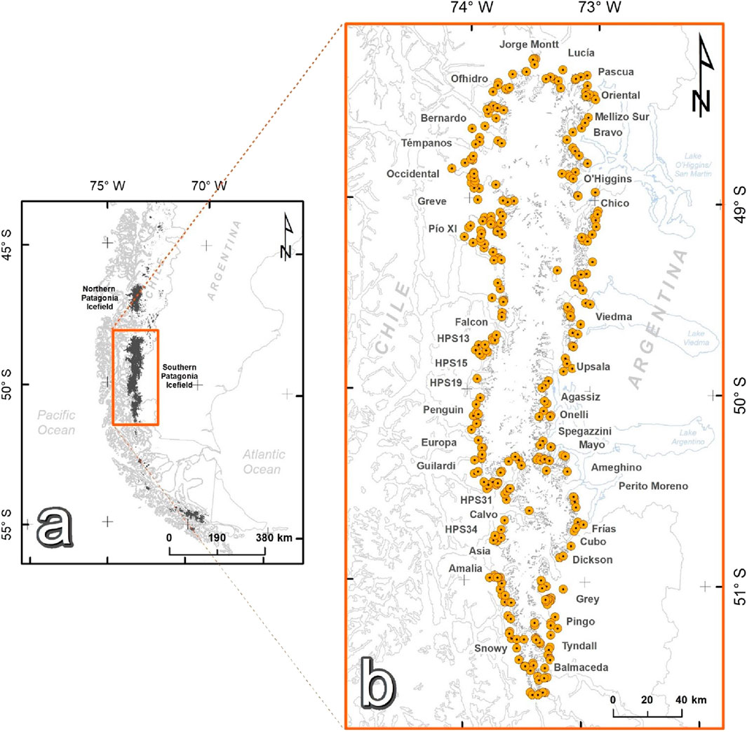
Figure 1. Map (a) shows the location of the Northern Patagonia Icefield (NPI) and Southern Patagonian Icefield (SPI). Map (b) shows the location of the glacial lakes surrounding the Southern Patagonian Icefield (SPI) (indicated by orange circles). Dark grey labels identify the main outlet glaciers of the SPI.

2 Data and methods

2.1 Data sources and glacial mapping criteria

In this study, glacial lakes were mapped only if they were located within or immediately adjacent to the 1945 extent of the SPI outlet glaciers. This search area was chosen as it likely contained lakes that had experienced the most significant changes during the observation period (Loriaux and Casassa, 2013). The boundaries of the outlet glaciers in 1945 were derived from a 1:250,000 scale map created and published in 1954 by the Chilean Geographic Military Institute (Instituto Geográfico Militar, IGM). This map was based on the Trimetrogon aerial photographic survey conducted by the U.S. Army Air Force between December 1944 and March 1945. To enhance the accuracy of the analysis, original Trimetrogon aerial photographs were also utilized, as there were some inaccuracies in the maps.

To complete the multi-temporal glacial lake inventory for the SPI, a total of 93 Landsat and Sentinel-2 satellite images were used, with acquisition dates between 1986 and 2023 (Table 1). The satellite imagery used was selected based on image availability and the presence of snow cover, cloud cover and mountain shadowing. All images were obtained from the United States Geological Survey’s (USGS) Earth Explorer interface (https://earthexplorer.usgs.gov/). Named lakes were identified using 1:50,000 maps available from the IGM and reports from the Argentine Geographic Institute.

Table 1

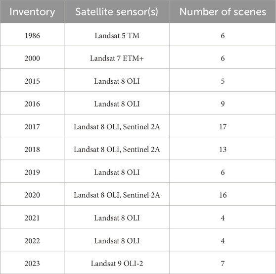
Table 1. Summary of the Landsat and Sentinel-2 satellite imagery used for the compilation of the multi-temporal glacial lake inventory (1986–2023).

Each glacial lake mapped was characterized by several quantitative and qualitative attributes, including an identification ID code, name (if available), lake type, central coordinates, elevation, and surface area. Following the guidelines of Wilson et al. (2018) and Carrivick and Tweed (2013), glacial lakes were categorized into three sub-types based on the nature of their impounding dams (Figure 2): (1) moraine-dammed lakes (encompassing all subtypes of moraine dams); (2) bedrock-dammed lakes (situated within bedrock over-deepenings); and (3) ice-dammed lakes (impounded by ice). This categorization was done through visual analysis supported by geomorphological observations made by Davies et al. (2020). These observations included detailed maps of the moraines surrounding the SPI, which were used to help identify the composition of the dams.

Figure 2

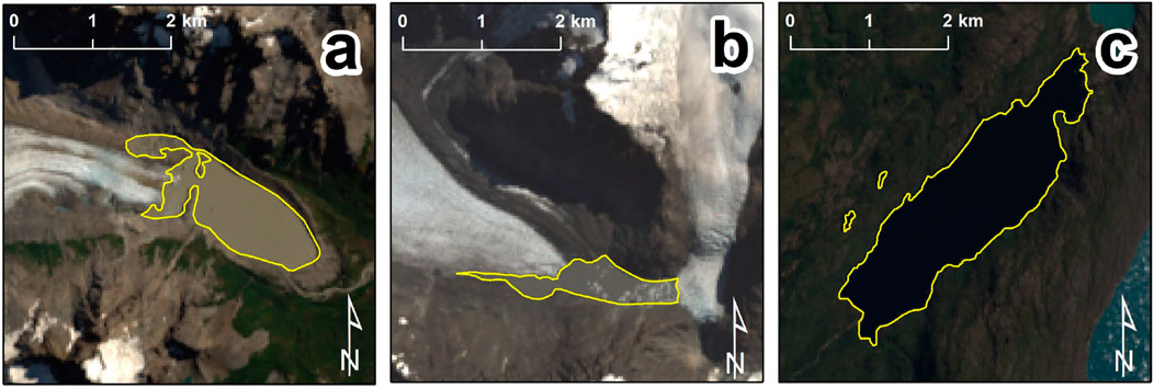
Figure 2. Examples of glacial lakes classified as: (a) moraine-dammed (49.32°S, 73.00°W); (b) ice-dammed (49.70°S, 73.15°W); and (c) bedrock-dammed (48.27°S, 73.49°W). Images are natural colour composite pan-sharpened Landsat eight images. The yellow outlines represent lake margins from the 2021 inventory.

To characterize glacial lake changes at a sub-annual scale between 2015 and 2023, when a significant change was observed, we included additional images to increase the temporal resolution of the inventory. However, due to the temporal resolution of the satellite data used (e.g., 16 days for Landsat eight and 5–10 days for Sentinel-2 data), cloud cover and other data quality issues, often the temporal resolution achieved was not high enough to properly characterize the observed changes. Lakes Argentino (1,368.5 ${\text{km}}^2$), Viedma (1,211.5 ${\text{km}}^2$), and O’Higgins/San Martín (1,042.6 ${\text{km}}^2$), which are located on the eastern margin of the SPI (Figure 1), were excluded from the inventory, as they are several orders of magnitude larger than any other glacial lake considered in this study. Supraglacial lakes were also excluded due to their seasonal nature. A small number of lakes $(<30)$ were not mapped in some images due to localized cloud cover.

2.2 Glacial lake delineation

Glacial lakes were mapped in this study using a semi-automated approach, combining the use of the normalized difference water index (NDWI) (McFeeters, 1996) and manual editing. The NDWI is calculated following Equation 1:

$NDWI=\frac{P_{\text{green}}-P_{\text{NIR}}}{P_{\text{green}}+P_{\text{NIR}}}(1)$

where $P_{\text{green}}$ and $P_{\text{NIR}}$ denote the green and near-infrared (NIR) bands, respectively.

The Normalized Difference Water Index (NDWI) has been widely used in glacial lake inventories (Huggel et al., 2002; Zhang et al., 2021). The effectiveness of the NDWI for glacial lake mapping can be hindered by image quality issues, including snow, ice, cloud cover, and mountain shadowing. Shadowed areas are common in mid-latitude mountain regions such as Patagonia and exhibit a spectral signature similar to that of glacial lakes with low turbidity, leading to potential misclassification (Gardelle et al., 2011; Loriaux and Casassa, 2013). In this study, shadow areas were discriminated from each other through the use of a slope map derived from the 2000 Shuttle Radar Topography Mission (SRTM) Digital Elevation Model (DEM) at a 90 m spatial resolution. This slope map was visually inspected together with the satellite imagery to correct any potential misinterpretations (Figure 3).

Figure 3

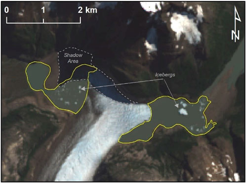
Figure 3. Example of the high variability of the spectral signature of glacial lakes due to the presence of icebergs and shadowing. Natural color composite image acquired on 3 March 2021. The yellow outlines represent lake margins from the 2021 inventory.

Estimating the mapping errors associated with the glacial lake area calculations is challenging without using high-resolution reference data. Several factors influence this estimation, such as the spatial resolution of the imagery (e.g., Landsat = 15–30 m and Sentinel-2 = 10 m), geometric accuracy of the images (e.g., Landsat = 15 m and Sentinel-2 = 10 m), the expertise of the operator performing the classification, and specific image quality issues previously reported (Paul et al., 2013; Wilson et al., 2018).

Following these considerations, we adopted the error estimation approach proposed by Hanshaw and Bookhagen (2014), as adapted by Lesi et al. (2022). This methodology estimates error as a function of the number of edge pixels in a lake polygon, with adjustments to account for duplicated nodes. Key parameters include the total number of nodes in the lake polygon $(N_{\text{total}})$, image spatial resolution $(G)$, lake perimeter $(P)$ and a coefficient of 0.6872, which reflects that approximately 69% of pixels along lake edges are subject to classification uncertainty.

The equation used to estimate the error is:

${\text{Error}}_{1\sigma }=\left(\frac{P}{G}-N_{\text{int}}\right)\times 0.6872+\frac{G^2}{2}(2)$

where,

$•$ ${\text{Error}}_{1\sigma }$ is the 1$\sigma$ error in square meters,

$•$ $P$ is the lake perimeter in meters,

$•$ $G$ is the spatial resolution of the imagery (e.g., 10 or 30 m),

$•$ $N_{\text{int}}$ is the number of inner nodes of the lake polygon, which corresponds to nodes at angles greater than 180° when measured from the inside of the lake.

In the original formulation, the number of edge pixels corresponds to the fraction $P/G$. However, corner pixels at interior nodes were counted twice, leading to an overestimation of uncertainty. To correct for this, Lesi et al. (2022) introduced the term $N_{\text{int}}$ in Equation (2), producing a correct count of edge pixels.

Following Lesi et al. (2022), we use two different expressions to calculate $N_{\text{int}}$ depending on whether or not the polygon contains internal islands.

For polygons without islands, we estimate the number of inner nodes following Equation 3 as:

$N_{\text{int}}=\frac{N_{\text{total}}-4-1}{2}(3)$

where $N_{\text{total}}$ is the total number of nodes in the polygon, and the subtractions account for four corner nodes and one duplicated endpoint.

For polygons with islands, we apply Equation 4 as follows:

$N_{\text{int}}=\frac{N_{\text{total}}-\left(N_{\text{island}}+1\right)\times 5}{2}(4)$

where $N_{\text{island}}$ is the number of internal islands. Each island is assumed to contribute five nodes (four corners plus one duplicated node).

The total number of nodes for each lake delineation was computed using the exterior.coords function from the GeoPandas package (Jordahl et al., 2020) in Python 3.9.

Finally, the relative uncertainty $D$ is computed following Equation 5 as:

$D=\frac{{\text{Error}}_{1\sigma }}{A}\times 100\%(5)$

where $A$ is the lake area in square meters.

Individual glacial lakes were assigned unique identification (ID) numbers. To consistently associate the same ID with corresponding lake outlines identified from different years, an equivalent circular area was first calculated for each lake. This area represents the space a circular lake with the same perimeter as the mapped lake would occupy, allowing for the standardization of irregular lake shapes into a comparable metric. Lakes were then matched by comparing their centroids with those of lakes identified in previous time periods. If the centroid of a lake fell within the equivalent circular area of a previously mapped lake, it was then considered to be the same lake. All lakes that did not meet this criterion were assigned ID letters along with their emergence year (year ID), unless they already had a name. If a lake did not fit within the reference circular area, we evaluated whether the areas of both lakes intersected. If an intersection existed, the compared lake was kept as the reference unless it already had a name. In cases where a name was present, the existing name was preserved, and the lake was renamed only if no reference lake was matched.

To assess area changes, we compared the calculated area of each lake across different time periods. If the most recent area measurement fell within the error range of the earlier measurement, we considered the lake’s area unchanged. If the most recent area exceeded the previous measurement and fell outside the error margin, we concluded that the lake had increased in size. Otherwise, we determined that the lake’s area had decreased.

2.3 Volume estimation

To estimate glacial lake volume, we used the empirical area–volume relationship proposed by Shugar et al. (2020) as a starting point. This approach employs a mixed model with different equations for small and large lakes, using a threshold area of 0.5 km² to divide the two groups. As this method is widely applied at the global scale, it provides a useful benchmark for evaluating its applicability to glacial lakes in the Southern Patagonian Icefield (SPI). The equations used by Shugar et al. (2020) are described in Equations 6–8.

$\text{For small lakes}\left(A\le 0.5{\text{km}}^2\right):\ln \left(V\right)={\beta }_0+{\beta }_1\cdot \ln \left(A\right)+\epsilon (6)$

$\text{Back}-\text{transformed for volume prediction:}V=e^{{\beta }_0}\cdot A^{{\beta }_1}\cdot e^{\epsilon }(7)$

$\text{For large lakes}\left(A>0.5{\text{km}}^2\right):V=k_1\cdot A^{k_2}+\epsilon (8)$

where $V$ is lake volume in km³;, $A$ is lake area in km²;, and $\epsilon$ is the residual error.

Given the high proportion of small lakes $(<3{\text{km}}^2)$ in our inventory, we found it necessary to adjust the model to the characteristics of Patagonian glacial lakes. Therefore, we constructed a new mixed model (V_pow–poly3), which combines a power-law function for small lakes and a third-order polynomial for larger lakes. This model is an empirical fit to the 120 lakes of known volume used by Shugar et al. (2020) and aims to improve volume estimation accuracy, particularly for smaller lakes which the model used by Shugar et al. (2020) tends to overestimate.

The best model was found by minimizing the misfit using the coefficient of determination $R^2$, the sum of squares due to error (SSE) and the root mean squared error (RMSE), these quantities were defined in Equation 9 as:

$R^2=1-\frac{SSE}{SST}(9)$

where SST is the total sum of squares around the mean. The SSE is given by Equation 10 as:

$SSE={\displaystyle \sum _{i=1}^N}{\left(V_i-{\widehat{V}}_i\right)}^2(10)$

and the SST by Equation 11 as:

$SST={\displaystyle \sum _{i=1}^N}{\left(V_i-\bar{V}\right)}^2(11)$

where $V_i$ is the observed volume of the $i$-th lake, $\widehat{V_i}$ is the estimated volume, and $\bar{V}$ is the mean volume of the $N$ data points evaluated.

The root mean squared error (RMSE) was calculated by Equation 12 as:

$RMSE=\sqrt{\frac{SSE}{N}}(12)$

The fitting process was carried out using the robust least absolute residuals (LAR) algorithm in Matlab Center (2021a), and applied to the entire dataset for each polynomial.

2.4 Characterization of GLOFs from ice-dammed lakes

Lakes have a natural water level variation resulting from changes in water input. However, on ice-dammed lakes, these variations are much larger due to changes in the ice dam and GLOFs that can fully drain a lake due to the formation of a subglacial or englacial channel. When a significant decrease in area was observed in an ice-dammed lake, we assumed it was due to a GLOF, and we chose to timestamp the event using the date of the image in which the area reduction was detected. However, it might have happened anytime between the date of that image and the previous one in the inventory. For each GLOF, we used our area-volume empirical relationship to calculate the water volume evacuated. O’Connor et al. (2001) developed an empirical model correlating this evacuated volume with the peak discharge of the GLOF. We used this model to estimate the peak discharge of all drainage events identified. Both evacuated volume and peak discharge must be considered lower bounds, as it is likely that our images captured the lake before it was fully drained or after it had partially refilled. The peak discharge was estimated using Equation 13 as follows:

$Q_{\text{max}}=0.054\cdot V_{\text{max}}^{0.66}(13)$

where $V_{\text{max}}$ is the total volume drained in cubic meters $m^3$. The processes that trigger the sudden drainage of ice-dammed lakes are complex and have been related to changes in ice thickness, lake bathymetry, calving activity, subglacial water pressure, and thermal conditions, among other factors (Roberts, 2005; Clague and Mathews, 1973; Clague and O’Connor, 2021). With this in mind, the GLOF peak discharge estimations presented here are likely to include large uncertainties and, therefore, should only be considered first-order approximations.

3 Results

3.1 Glacial lake volume estimation

Our database shows that 85% of the inventoried lakes have areas between 0 and 3 ${\text{km}}^2$. Various methods exist to estimate lake volume, including the mixed model proposed by Shugar et al. (2020). Shugar et al. (2020)’s model is innovative because it applies different area-volume scaling relationships for lakes of different sizes. However, 84% of the lakes they studied had areas below 0.5 ${\text{km}}^2$, a point where the mixed model applied exhibited a discontinuity, resulting in similar volume estimates for lakes with significantly different areas. This issue was especially serious for lakes with areas of around 2.82 ${\text{km}}^2$.

Given the area distribution in our inventory and the issues caused by this discontinuity, a new relationship was developed in this study to improve model accuracy, particularly for lakes with areas smaller than 3 ${\text{km}}^2$. To achieve this, two polynomial models are proposed based on the same dataset used by Shugar et al. (2020):

$V_{\text{poly}2}=f_2\left(A\right)=p_{21}{A}^2+p_{22}(14)$

$V_{\text{poly}3}=f_3\left(A\right)=p_{31}{A}^3+p_{32}(15)$

where $V_{\text{poly}2}$ and $V_{\text{poly}3}$ represent lake volume estimates in km³; for a given lake area $A$ in ${\text{km}}^2$, and $p_{21},p_{22},p_{31},p_{32}$ are the regression parameters. Both models display similar behaviour to that shown for other glacial lake power area-volume relationship found in the literature (e.g., Iturrizaga, 2014; Cook and Quincey, 2015; Wilson et al., 2018; Buckel et al., 2018), $f_2(0)=0$ and $f_3(0)=0$, with strictly increasing slopes for $A>0$, where $f_2^{\prime }(A)>0$ and $f_3^{\prime }(A)>0$ when $p_{21},p_{31}>0$ and $p_{22},p_{32}\ge 0$.

The second-order polynomial model, $f_2$, has also been used by O’Connor et al. (2001) for area-volume relationships in moraine-dammed lakes. With the third-order polynomial defined in Equation 14 and the conditions on $p_{31}$ and $p_{32}$, we ensured ${f^{″}}_3(A)>0$ to fix the inflection point at $A=0$, guaranteeing the convexity of $f_3$ for all $A\ge 0$.

The resulting models are shown in Figure 4, and the fitting parameters in Table 2. Both models show a reasonable fit to the lake volume data, although $V_{\text{poly}3}$ provides better $R^2$ and RMSE values than $V_{\text{poly}2}$, along with a lower $SSE$ for lakes with areas smaller than 3 ${\text{km}}^2$. However, from the residual analysis, a systematic overestimation was observed for lakes larger than 0.57 ${\text{km}}^2$ in $V_{\text{poly}3}$, while $V_{\text{poly}2}$ showed an overestimation for lakes larger than 0.35 ${\text{km}}^2$, which represent 94% of the lakes in our database.

Figure 4

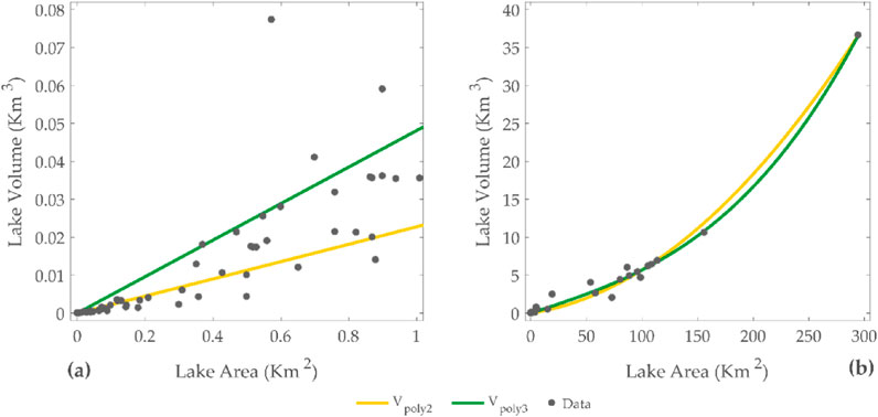
Figure 4. Models $V_{\text{poly}2}$ and $V_{\text{poly}3}$ for (a) lakes areas $<1{\text{km}}^2$ (66% of the dataset) and (b) all the dataset (122 glacial lakes).

Table 2

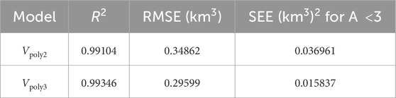
Table 2. Statistical results for $V_{\text{poly}2}$ and $V_{\text{poly}3}$ models.

Even though both models introduce some bias in estimating smaller lakes, the statistics for the third-order polynomial suggest that $V_{\text{poly}3}$ may be more useful for prediction. However, the overestimation of the small lakes by $V_{\text{poly}3}$ is addressed by using a mixed model, as proposed by Shugar et al. (2020). This model avoids discontinuities in the glacial lake volume estimation and better fits lakes with areas smaller than 3 ${\text{km}}^2$.

The mixed model developed consists of two components that require an intercept area value of at least 0.57 ${\text{km}}^2$. In this mixed model, $V_{\text{poly}3}$ represents the second part, while the first part is based on the classic power area-volume relationship approach, which we established as follows:

$V_{\mathit{pow}}=f_1\left(A\right)=k_1{A}^{k_2}(16)$

where $V_{\text{poly}3}$ is the lake volume estimation in ${\text{km}}^3$, A is the lake area in ${\text{km}}^2$, and $k_1$ and $k_2$ are the regression parameters.

Based on Equations 15, 16, the mixed model that was evaluated was set out as follows:

$V_{\mathit{pow-poly3}}=\left\{\begin{array}{cc}{k}_1{A}^{k_2}\hfill & A\le A_{13}\left({\text{km}}^2\right)\hfill \\ p_{31}{A}^3+p_{32}A\hfill & A>A_{13}\left({\text{km}}^2\right)\hfill \end{array}\right.(17)$

where $(A_{13})$ represents the mixed model transition point, which corresponds to the intercept between $(V_{\text{pow}})$ and $(V_{\text{poly}3})$. This can be achieved for lake areas greater than zero by selecting a specific subset of the data.

3.1.1 Finding the best volume estimation mixed model

To address the bias in small lakes and improve the accuracy of the third-order polynomial model $(V_{\text{poly}3})$ outlined in Section 3.1, this study aims to find the best mixed model, as described in Equation 17, ensuring that its transition point occurs at $A_{13}\ge 0.57$ ${\text{km}}^2$.

The process began by sorting the lake area data in ascending order and selecting consecutive subsets of area-volume pairs. This process was started with lakes that have areas ranging from 0 to 0.57 ${\text{km}}^2$, progressively adding the next data point until the entire dataset was covered. For each subset, the robust Bisquare fitting algorithm available in Matlab was used Center (2021a) to find the best fit for Equation (7). This algorithm helped reduce the influence of any outliers or variability in the dataset, which is particularly important for small lakes where errors can be more pronounced.

For each of these fitted subsets, the intersection point between the power model $(V_{\text{pow}})$ and the third-order polynomial model $(V_{\text{poly}3})$ was first calculated. The $R^2$ and RMSE values for the entire mixed model (combining both equations) were then computed using the complete dataset. This process was repeated for all subsets to identify the point where $R^2$ was maximized and RMSE was minimized, ensuring the best overall fit for the model.

The optimal transition point was found to be $A_{13}=1.3336{\text{km}}^2$. Table 3 compares the statistical results of this best-fitting mixed model $(V_{\text{pow}-\text{poly}3})$ with those of the original mixed model by Shugar et al. (2020) $(V_{\text{pow}-\text{pow}})$. Although the $R^2$ values for both models are similar, $V_{\text{pow}-\text{poly}3}$ shows an improvement in RMSE and SSE for lakes with areas less than 3 ${\text{km}}^2$. This indicates that the main source of error in volume estimation is for larger lakes, where less data is available (only 20% of the dataset corresponds to lakes with areas greater than 3 ${\text{km}}^2$).

Table 3

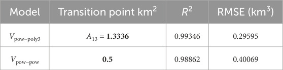
Table 3. Statistical results for evaluated models.

By analyzing the residuals of the best-fitting model, it was confirmed that $V_{\text{pow}-\text{poly}3}$ resolves the overestimation bias seen in $V_{\text{poly}3}$ for lakes smaller than 0.57 ${\text{km}}^2$, making it the most suitable model for estimating lake volumes in the glacial lake database presented here.

To improve the accuracy of lake volume estimation, particularly for lakes smaller than 3 ${\text{km}}^2$, a mixed model was developed by combining a power-law function with a third-order polynomial model. The threshold area $(A_{13})$ was determined to optimize the model fit, ensuring a smooth connection between both functions. The resulting mixed model follows Equation 18 defined as:

$V_{\mathit{pow-poly3}}=\left\{\begin{array}{cc}{k}_1{A}^{k_2}\hfill & A\le A_{13}\left({\text{km}}^2\right)\hfill \\ p_{31}{A}^3+p_{32}A\hfill & A>A_{13}\left({\text{km}}^2\right)\hfill \end{array}\right.(18)$

where $A_{13}=1.336$ ${\text{km}}^2$, represents the transition point between the power-law model $(V_{\text{pow}})$ and the third-order polynomial model $(V_{\text{poly}3})$. The optimal transition point was found by maximizing $R^2$ and minimizing RMSE. Compared to the original mixed model proposed by Shugar et al. (2020), our approach showed improved accuracy for lakes smaller than 3 ${\text{km}}^2$, which represent 94/% of the dataset. Residual analysis indicates that $V_{\text{pow}-\text{poly}3}$ corrects the overestimation bias observed in $V_{\text{poly}3}$ for lakes smaller than 0.57 ${\text{km}}^2$. In addition, the model achieves a better fit for larger lakes, reducing errors in volume estimation.

Figure 5 illustrates the comparison between the mixed model and the model by Shugar et al. (2020), which includes 122 glacial lakes with in situ measurements in its dataset. The differences in lake volume estimations are more pronounced in smaller lakes, where the new model corrects overestimation and better captures variations in volume.

Figure 5

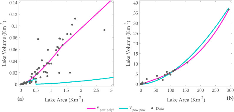
Figure 5. Comparison between mixed models $V_{\text{pow}-\text{poly}3}$ and $V_{\text{pow}-\text{pow}}$ from Shugar et al. (2020) for: (a) lakes areas $<3({\text{km}}^2)$ (80% of the dataset) and (b) all the span in dataset (122 glacial lakes).

In addition to estimating lake volume using the mixed model $V_{\text{pow}-\text{poly}3}$ presented in Equation 8, the predint command in Matlab Center (2021b) was used to compute the prediction intervals at the confidence level of 95% to quantify the uncertainty in the estimation. The procedure was carried out by evaluating each part of the mixed model, i.e., Equations 7,12, for every lake in the database $>A_{13}({\text{km}}^2)$ and $\le A_{13}({\text{km}}^2)$, respectively. After performing these calculations, the estimated volumes and their corresponding prediction intervals were added according to each dam classification by year. A value of zero was assumed for any negative values in the lower bound of the prediction interval.

3.2 Spatial and altitudinal distribution of glacial lakes in 2023

In total, 313 glacial lakes were detected in the 2023 inventory (Figure 6; Table 4), covering an area of 639.09 ${\text{km}}^2$ and storing an estimated 34.84 ${\text{km}}^3$ of water. Of the lakes identified, moraine-dammed lakes accounted for the largest portion (165; 52.72% of total), followed by bedrock-dammed lakes (76; 24.28% of total) and ice-dammed lakes (72; 23% of total). In terms of area, moraine-dammed lakes accounted for 56.43% of the total, followed by ice-dammed lakes (34.87%) and bedrock-dammed lakes (8.70%). Despite their smaller area, ice-dammed lakes were found to have a similar total volume (15.65 ${\text{km}}^3$) to moraine-dammed lakes (16.77 ${\text{km}}^3$). In terms of their morphology, most lakes were found to be elongated and aligned with their associated glacier tongue due to the influence of glacial topography and the direction of ice flow. This was particularly the case for moraine-dammed lakes. However, ice-dammed lakes, which typically occur at higher elevations, were found to exhibit more irregular shapes, both spatially and temporally. This is due to the inherent instability and variable geometry of the ice dams that impound them, which, combined with the large fluctuations in water level observed for this type of lake, cause significant changes in lake shape between observations. Ice-dammed lakes primarily develop in areas that have recently undergone deglaciation, causing them to change their orientation and shape along with fluctuations in the surrounding glaciers. The most significant ice-dammed lakes, such as Bernardo and Pío XI, are located in the northwest part of the SPI and parallel to the main mountain range along the SPI.

Figure 6

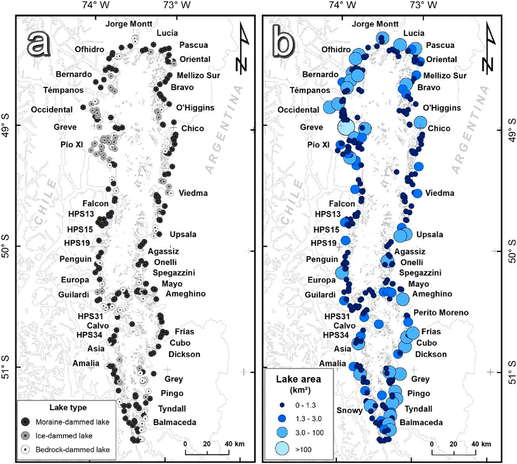
Figure 6. Spatial distribution of the 313 glacial lakes observed in 2023 by type (a) and size (b). The names correspond to the SPI main glaciers. Lakes Argentino, Viedma and O’Higgins/San Martín were excluded from the inventory as mentioned in the data and methods section (subsection 2.1).

Table 4

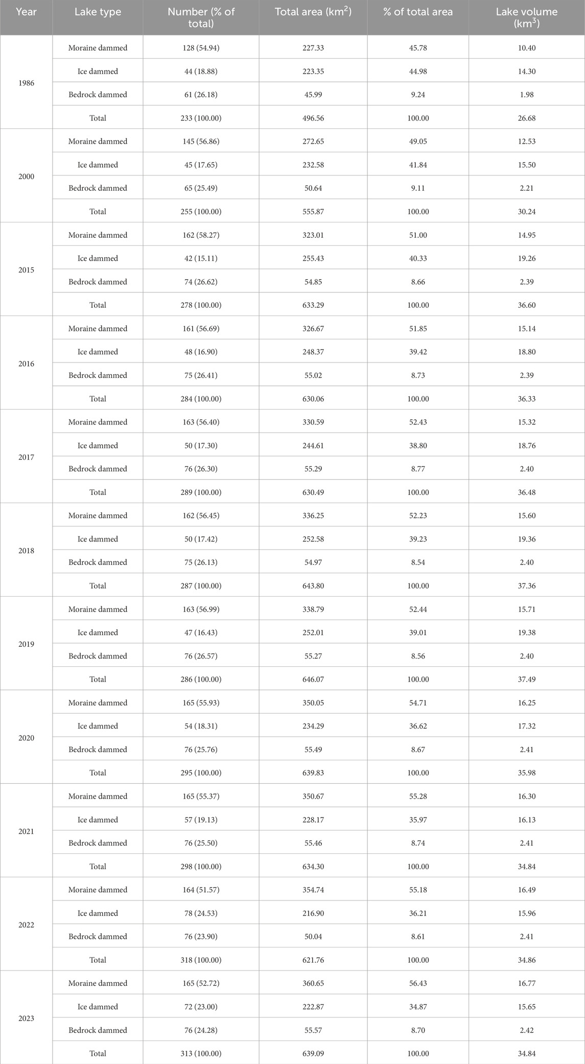
Table 4. Main characteristics (number, area, and water volume) of the glacial lakes inventoried between 1986 and 2023.

In terms of their spatial distribution, smaller glacial lakes ($<3$ ${\text{km}}^2$) are shown to be uniformly distributed around the periphery of the SPI, occupying previously deglaciated glacial valleys (Figure 6). In contrast, larger lakes ($>3$ ${\text{km}}^2$) are more concentrated along the southeast and northwest periphery of the SPI. With respect to area, 78.27% of the glacial lakes detected (n = 245) are smaller than 1.3 ${\text{km}}^2$. Lake Greve stands out as the largest lake in the 2023 inventory, representing 28% of total area and covering 180.52 ${\text{km}}^2$ (13.84 ${\text{km}}^3$). Lake Greve is an ice-dammed lake located in the northwest section of the SPI and is dammed by Pío XI Glacier. The elevation analysis shows that 91% of the glacial lakes mapped are located below 800 m. a.s.l (Figure 7).

Figure 7

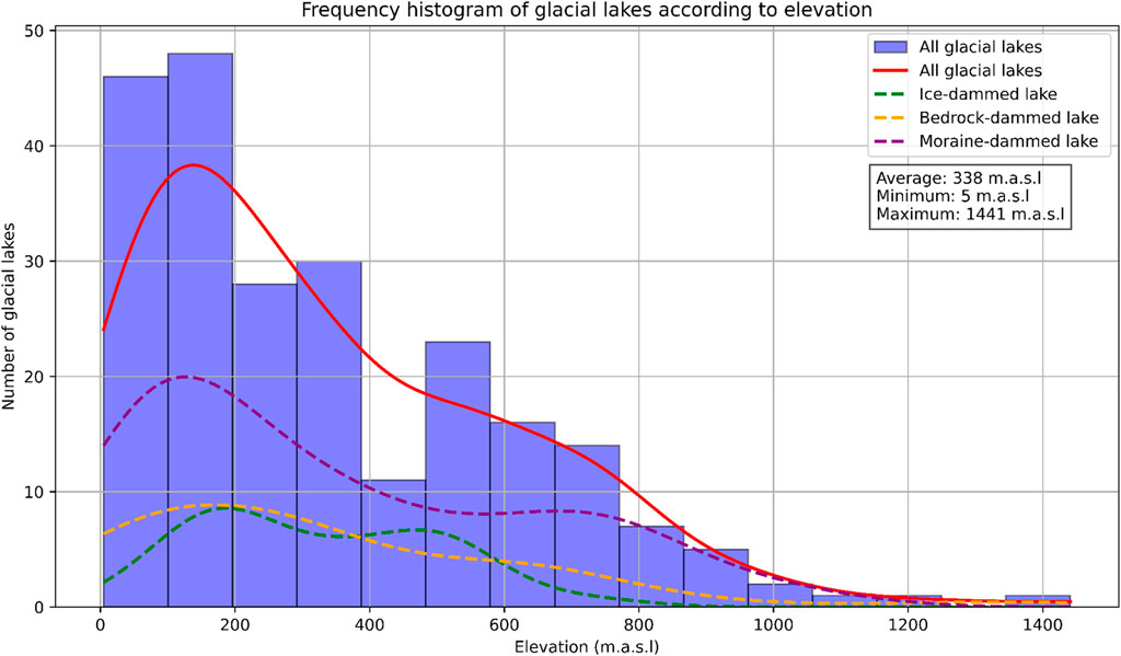
Figure 7. Frequency histogram of glacial lakes according to elevation.

3.3 Evolution of glacial lakes between 1986 and 2023

The assessment of the temporal evolution of glacial lakes, based on a comparison of the 1986, 2000, and 2015–2023 inventories (Table 5), showed that the number of glacial lakes increased from 233 in 1986 to 313 in 2023, reflecting a 34% rise. The total surface area expanded from 496.56 km²; in 1986 to 639.09 km²; in 2023, representing a 29% increase over the same period. In comparison, the total lake volume increased by 31%, from 26.68 ${\text{km}}^3$ in 1986 to 34.84 ${\text{km}}^3$ in 2023, with slight interannual variations. Throughout the observation period, 2019 was identified as having the largest total glacial lake area of 646.07 ${\text{km}}^2$ (Table 5). This total area shrank by 1%–639.09 ${\text{km}}^2$ by 2023.

Table 5

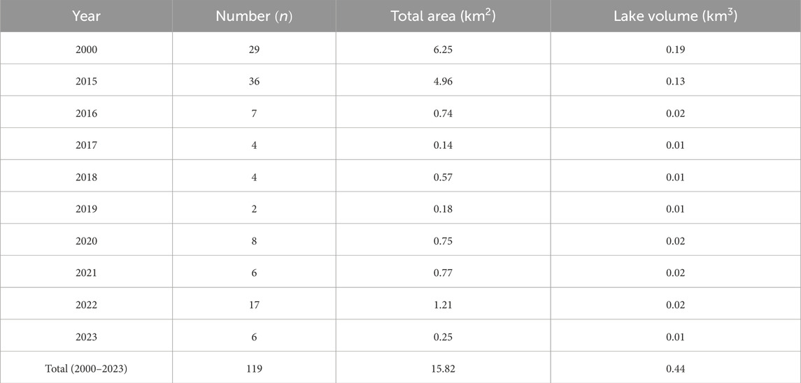
Table 5. Number, area and water volume of new glacial lakes identified between 2000 and 2023.

Overall, the mapped glacial lakes exhibited various changes, including expansion, coalescence, shrinkage, disappearance, and detachment from their parent glaciers. As expected, bedrock-dammed lakes demonstrated greater stability, as they are typically smaller and situated in geomorphologically stable basins. In contrast, ice-dammed lakes showed high areal variability, while the most significant growth was observed in moraine-dammed lakes (Figure 8).

Figure 8

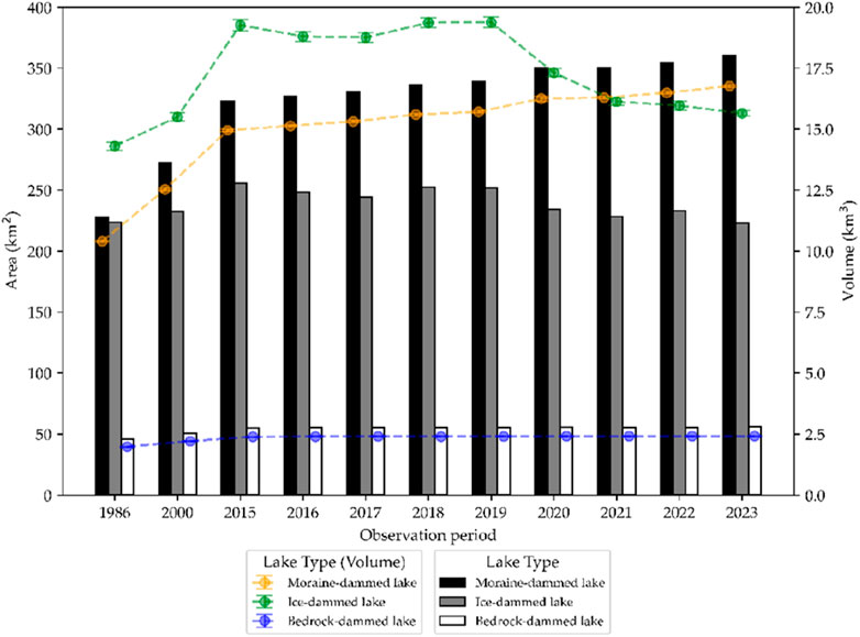
Figure 8. Behavior of the three types of glacial lakes: (a) moraine-dammed (black column); (2) ice-dammed (grey column); and (3) bedrock-dammed (white column). Glacial lake volume is represented by the orange, green and purple points, respectively.

Throughout the 37-year observation period (Table 5), a total of 352 lakes were mapped (233 lakes in 1986 and a further 199 lakes mapped between 2000 and 2023). Between 2000 and 2023, the newly emerged lakes accounted for a total area and volume of 15.82 ${\text{km}}^2$ and 0.44 ${\text{km}}^3$, respectively. Interestingly, the rate of glacial lake emergence was observed to triple between 2015 and 2023 (an average of 6.7 lakes emerging per year) compared to the 1986–2015 period (an average of 2.2 lakes emerging per year). Within this most recent period (2015–2023), the contrast between 2021 and 2022 is notable, with 17 new lakes emerging, which is far greater than the average of 5.8 lakes emerging per year over the entire observation period.

The analysis of the evolution of lakes that existed in 1986 shows that, in 2023 44% maintained their area (n = 155), 29% increased in area (n = 102), 15% reduced their area (n = 52) and 12% disappeared (n = 44). All the disappeared lakes were dammed by ice. Overall, moraine-dammed lake tended to increase their area while bedrock-dammed lakes tended to maintain their area (Figure 9).

Figure 9

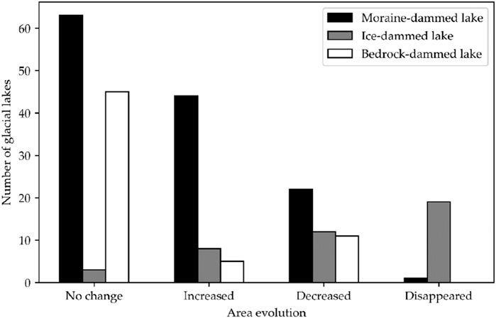
Figure 9. Evolution of the number of glacial lakes studied between 1986 and 2023: moraine-dammed lake (black), ice-dammed lake (gray) and bedrock-dammed lake (white). This figure excludes the six new lakes identified in 2023, as they have no reference for establishing a trend.

3.3.1 Type and evolution of new glacial lakes

Between 2000 and 2023 (Figure 10; Table 5), a total of 119 new glacial lakes emerged. In general, an increase in new lakes is observed. Most of these newly created lakes fail to consolidate and thus were drained, although they filled up again in 2021.

Figure 10

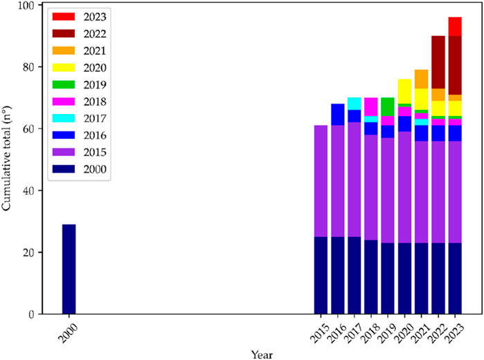
Figure 10. Number of new glacial lakes per year studied. Color codes represent the year of formation of the glacial lakes.

These newly formed lakes cover a total area of less than 1.3 ${\text{km}}^2$ and are uniformly distributed around the SPI (Figure 11). The largest of these lakes (with individual areas $>0.6$ ${\text{km}}^2$) appeared on or before 2015. Since then, only smaller lakes ($<0.6$ ${\text{km}}^2$) have appeared. From 2016 onwards, the emergence of new lakes has been primarily associated with the glacier systems of Pío XI, Bernardo-Témpanos, O’Higgins-Chico, Viedma and Amalia glaciers. The six new lakes that emerged in 2023 were located in the northern periphery of the SPI and were all ice-dammed.

Figure 11

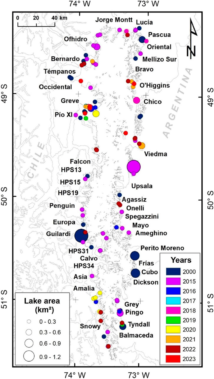
Figure 11. Size and spatial distribution of new glacial lakes per year of detection. The names correspond to the SPI main glaciers. Color codes refer to those shown in Figure 10.

Regarding the newly formed lakes identified between 2000 and 2023, the following observations were noted (Figure 12): Ice-dammed lakes proved to be the most unstable, with new ice-dammed lakes emerging almost annually from 2016 onwards, but then disappearing in some cases due to rapid drainage events. New lakes associated with ice-dammed lakes tend to disappear rapidly. This instability was evidenced by the GLOF events recorded in 2016 and 2020, when several lakes experienced dramatic reductions in volume. There are also years, such as 2016 and 2022, in which large increases in ice-dammed lake area were observed, highlighting the dynamic nature of this type of glacial lake. In contrast, newly formed moraine-dammed lakes underwent a more gradual and uniform formation process, with lake growth being initiated as glaciers retreat into over-deepened basins and continuing until the parent glacier becomes detached. New moraine-dammed lakes were found to have formed in 2000, 2015, and 2016, and grew consistently up to 2023. Overall, the moraine-dammed lakes that emerged in 2000 have experienced the most significant growth, tripling in area and increasing their volume fivefold during the observation period. Lastly, bedrock-dammed lakes were found to be the most stable in terms of their area. The greater stability of bedrock-dammed lakes arises from the geological stability of their barriers over time. These lakes initially expanded in area by 21% between 2000 and 2015. This growth slowed significantly between 2015 and 2017, before remaining relatively stable between 2017 and 2023, with a slight reduction in area observed by 2023 (Figure 12). No new bedrock-dammed lakes appeared after 2016. The difference in the growth trends of each of the glacial lake types is shown in Figure 12 and is particularly evident between 2015 and 2023.

Figure 12

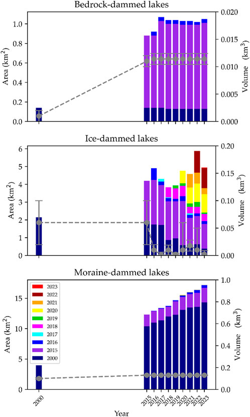
Figure 12. Evolution of new glacial lakes by types. Lake area and volume are represented by bars and dots, respectively. Color codes refer to those shown in Figure 10.

3.4 Recent dynamics of glacial lakes between 2015 and 2023

Between 2015 and 2023, several large GLOF events were observed in the SPI (Figure 13; Table 6). These events were primarily associated with ice-dammed lakes, which exhibit dynamic changes due to the formation of drainage channels through the ice that impounds them (Figure 14). One of the most significant GLOF events during the observation period occurred at the lake dammed by Bernardo Glacier (48.59°S, 73.80°W) on 30 May 2018, when a total of $\sim$0.59 ${\text{km}}^3$ of water drained, reaching a peak discharge of $\sim$33.3 ${\text{m}}^3$/s. A similar rapid drainage event was recorded on 15 October 2019, when $\sim$0.66 ${\text{km}}^3$ drained, accompanied by a peak discharge of $\sim$35.9 ${\text{m}}^3$/s (Figures 13, 14). This lake experienced periodic emptying each year and underwent a 53% reduction in area between 2015 and 2023. These changes are likely associated with the recent thinning of Bernardo Glacier, as geodetic measurements from 2000 to 2015/16 indicate a mean elevation change of −2.08 m ${\text{y}}^{-1}$. Another ice-dammed lake that has recently generated a large GLOF is Lake Greve. Dammed by Pío XI Glacier, Lake Greve was relatively stable until 27 June 2020, when $\sim$4.0 ${\text{km}}^3$ of water drained from the lake with a peak discharge of $\sim$116 ${\text{m}}^3$/s, making it the largest GLOF event to have occurred during the observation period. This lake also experienced new drainage events on 3 March 2021 and a smaller one on 4 June 2022.

Figure 13

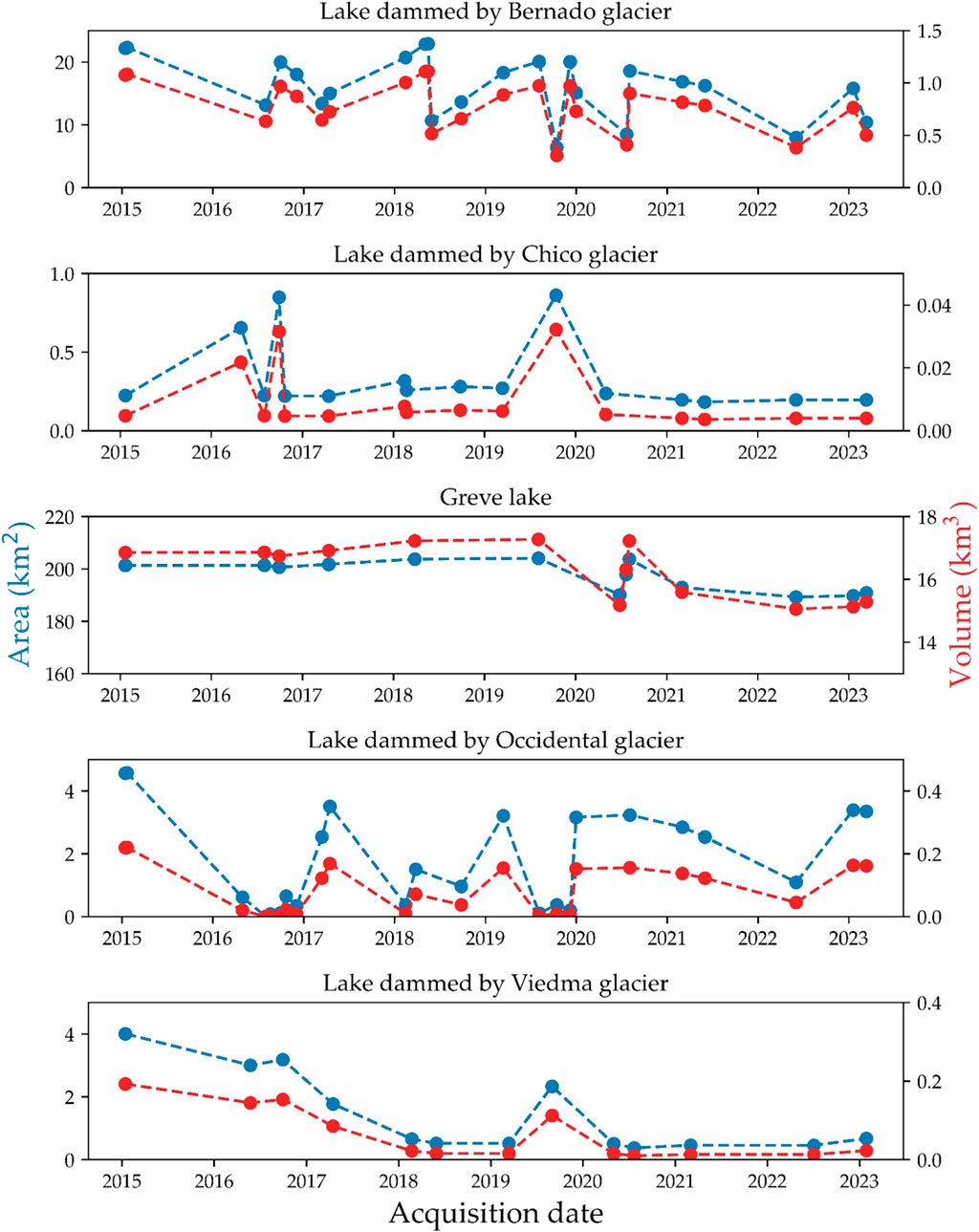
Figure 13. Recent dynamics of ice-dammed lakes studied between 2015 and 2023.

Table 6

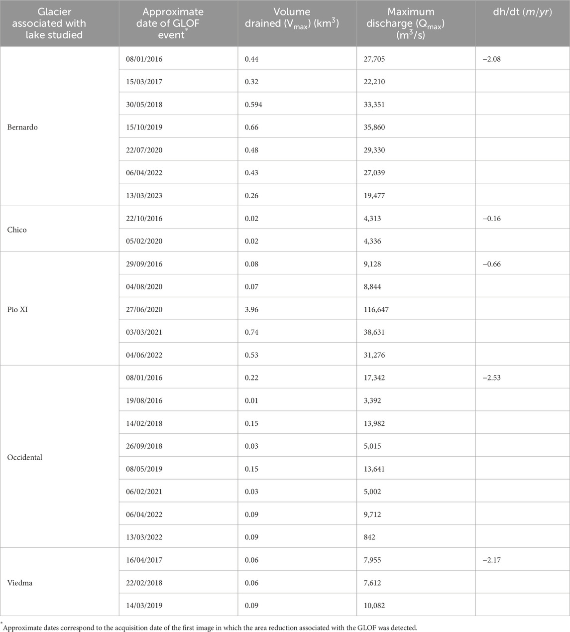
Table 6. Summary of the GLOF events observed at the lakes studied between years 2015 and 2023 with the mean dh/dt of their associated glacier as calculated by Malz et al. (2018).

Figure 14

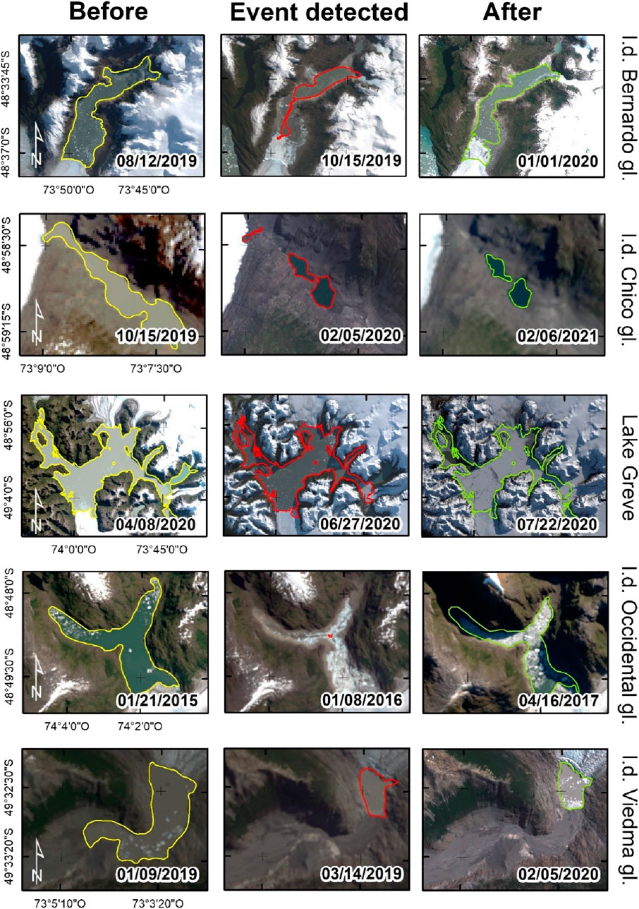
Figure 14. Before (yellow) and after (green) images of ice-dammed lakes with the largest dected changes in area. Lake area during the year of dection is shown in red.

Other important lakes that have produced GLOFs during the observation period are the lakes dammed by Chico, Viedma and Occidental glaciers. At the lake dammed by Chico Glacier (48.98°S, 73.13°W), cycles of lake filling and emptying are observed, where the lake during emptying periods becomes two smaller lakes. The lake dammed by Viedma Glacier (49.54°S, 73.05°W) has also undergone a number of filling and emptying cycles. This lake recorded its smallest area on 7 July 2020 (0.37 ${\text{km}}^2$) after a short period of expansion and filling, but has generally undergone a period of shrinkage, having reduced its area by 91% between 2015 and 2023. Lastly, the lake dammed by the Occidental Glacier (48.82° S, 74.04° W) was also observed to have experienced a number of drainage events (6 in total). The most notable of these events occurred on 8 January 2016, when $\sim$0.22 ${\text{km}}^3$ of water was drained at a peak discharge of $\sim$17.3 ${\text{m}}^3$/s, leaving only a small body of water behind, surrounded by a large number of grounded icebergs demarcating the former lake extent. Subsequent to this event, the lake continued with its filling and emptying cycles, with similar near-complete drainage events occurring in 2018 and 2019 (Figure 13).

It is worth mentioning that, as Figure 14; Table 6 show, all observed drainage events associated with ice-dammed lakes are indistinctly referred to as GLOF events hereafter. However, we have not identified the exact timing of each emptying episode.

4 Discussion

4.1 Methodological biases and limitations

Our methodological approach opened the possibility to produce a large and detailed dataset for studying glacial lakes and their evolution through time at decadal and annual scales. However, some of the processes we have studied, such as GLOFs, have annual periodicity and can exhibit significant changes at a daily scale. Consequently, our estimates of GLOF frequency may be influenced by the temporal availability of imagery. For example, years with more images have a higher likelihood of capturing a GLOF event. Similarly, the timing of image acquisition within a year may introduce bias, as ice-dammed lakes are more or less likely to be in a filled or drained state depending on the month. In the case of our lake volume calculations, for simplicity and due to the scarcity of validation data, we have treated all glacial lakes as equal, even though different processes have formed, which could result in differing area-volume relationships (Cook and Quincey, 2015). Nevertheless, as Shugar et al. (2020), this study neglects such differences and, therefore, the volume estimations reported must be considered first-order approximations.

4.2 Evolution of glacial lakes between 1986 and 2023

Between 1986 and 2023, the number, area, and volume of glacial lakes surrounding the SPI increased by 34%, 29%, and 31%, respectively. By 2023, this study identifies the existence of 313 lakes with a total volume of 34.84 ${\text{km}}^3$. The growth of glacial lakes in this area was primarily driven by the expansion of moraine-dammed lakes, resulting from the retreat of many of the SPI’s outlet glaciers. This retreat has led to the formation of new proglacial lakes and the enlargement of existing ones. These findings align with observations from other glaciated regions (Carrivick and Tweed, 2013). For the SPI, the results observed have three key implications. Firstly, it demonstrates that the meltwater storage capacity of the periglacial environment continues to increase. This storage not only has implications for global sea level assessments (Shugar et al., 2020), but may also affect the hydrological regime, sediment transport, water quality, and aquatic ecology of the many proglacial rivers originating from the SPI (Miserendino et al., 2023; Milner et al., 2017; Tweed and Carrivick, 2015; Tiberti et al., 2019). Secondly, the findings underscore the significant role that glacial lakes play in the glacier dynamics of the SPI. When in contact with their source glacier, glacial lakes can negatively impact glacier mass balance through subaqueous melting and the promotion of mechanical calving (King et al., 2019). The latter process is particularly relevant for the calving outlet glaciers of the SPI, some of which, such as Jorge Montt Glacier, have experienced periods of stability and rapid retreat in response to individual calving cycles that are decoupled from the local climate signal (Bown et al., 2019). These influences on glacier change in the SPI emphasize the need for continued monitoring of glacial lakes in this region into the future. Thirdly, southern Patagonia has been identified as a hotspot for GLOFs in the Andes, many of which have been generated by ice-dammed lakes and moraine-dammed lakes surrounding the SPI (Wilson et al., 2018). The continued emergence and expansion of lakes in this region has implications in terms of GLOF hazard and risk management, as discussed in the following sections, with up-to-date glacial lake inventories representing an important baseline dataset for subsequent GLOF hazard assessments (e.g., Iribarren Anacona et al., 2014).

Using geodetic methods, several studies have reported large ice mass losses for the SPI since the 1980s (Rignot et al., 2003; Jacob et al., 2012; Willis et al., 2012; Dussaillant et al., 2019) with Malz et al. (2018) reporting an overall specific mass balance of −0.941 $\pm$ 0.19 m w. e. ${\text{a}}^{-1}$ between 2000 and 2015/16. It is therefore unsurprising that the number and size of glacial lakes have increased over this period (Figure 11). However, the results presented reveal that the rate of glacial lake area expansion for the SPI has reduced considerably since 2015, reducing from an increase of 0.9% per year between 2000 and 2015 to 0.1% per year between 2015 and 2023. In contrast, the rate of glacial lake emergence was shown to more than triple between 2015 and 2023. However, this increase was driven by the appearance of new ice-dammed lakes, which tended to be smaller and undergo repeated phases of emptying and refilling, with no new moraine-dammed or rock-dammed lakes being observed since 2016. Given this, the reduction in the overall rate of glacial lake area expansion between 2015 and 2023 may suggest that (1) the availability of low gradient ice areas that facilitate lake growth during glacier retreat is reducing in the SPI; (2) glaciers are beginning to detach from their proglacial lakes (in doing so limiting their growth) and retreat to higher gradient portions of their basins and (3) most glaciers have retreated from their main (maybe change for LIA) frontal moraines. Therefore, no new moraine-dammed lakes can be formed. A similar but more pronounced reduction in the rate of glacial lake area expansion was also observed by Wilson et al. (2018) for Northern Patagonia Andes (36°–45°S) but for the earlier period of 2000–2016, with this region having been identified as having undergone more extensive rates of ice loss compared to the Southern Patagonia Andes (45°–55°S) (Wilson et al., 2018; Paul and Mölg, 2014).

From 1986 to 2023, 119 newly emerged lakes were recorded. Taking 1986 as a reference, we looked into the factors promoting the formation of new glacial lakes and the history of their development in relation to their dam type. Among these, bedrock-dammed lakes are usually smaller and offer relatively less variability with respect to area and volume after the peak achieved in 2017 (Figure 12).

On the other hand, ice-dammed lakes are much more variable. Although year after year, new ice-dammed lakes develop, their number is smaller, and they do not last long as opposed to the moraine and bedrock-dammed lakes (Figure 12). This characteristic reflects the observed variability in ice-dammed lakes driven by the drainage and refilling cycles associated with their ice-dam dynamics.

The non-linear nature of the area–volume relationship used means that a relatively small number of large lakes can contain a disproportionately high proportion of the total lake volume. On the other hand, small lakes are more numerous and, therefore, can have a large water volume. However, we found that small lakes are not numerous enough to compensate for their much smaller individual volumes, and a small number of large lakes monopolizes the water storage reported in our inventory. This was also true for ice-dammed lakes in the periods of 1986–2015 and 2019–2023, when large changes in lake size occurred in the two biggest ice-dammed lakes, dammed by the Pio XI and Bernardo glaciers. This is especially relevant as ice-dammed lakes pose the highest GLOF hazard. This highlights the importance of establishing continuous monitoring of these lakes, especially because of their sustained increase in number and size. New lakes formed between 1986 and 2023 account for around 15.82 ${\text{km}}^2$ out of an overall increase in lake area of 142.55 ${\text{km}}^2$. Moreover, this trend will likely persist in the coming decades, buoyed by the continued ice loss.

4.3 Glacial lake area-volume relationships: Evaluation of the mixed model approach

As discussed in section 4.2, lakes that have a larger surface area tend to have a disproportionately large impact on water storage. This relationship can also be found when using our mixed approach and has been pointed out in previous studies (e.g., Shugar et al., 2020; Loriaux and Casassa, 2013; Huggel et al., 2002; O’Connor et al., 2001; Cook and Quincey, 2015). In Figures 4, 5, we can see how the model calibrated by Shugar et al. (2020) and by us show how both the model calibrated by Shugar et al. (2020) and our own calibration produce increasingly steep curves for larger lakes, highlighting that lake volume grows disproportionately faster than area as lake size increases. This explains why two ice-dammed lakes, dammed by Pío XI and Bernardo glaciers, make the most significant contribution to the volume increases shown for 1986 to 2015 and from 2019 to 2023.

4.4 Ice-dammed lakes and drainage events

The Southern Patagonian Icefield (SPI) experienced significant variability regarding the formation and evolution of new glacial lakes, particularly in the northern section (Figure 11). The retreat of glaciers and climatic variations contributed to the dynamics of these areas, alongside the periodic creation and rapid disappearance of ice-dammed lakes due to drainage events likely associated with GLOF phenomena. This disappearance of ice-dammed lakes can be attributed to drainage that occurred by the thinning of the glacial dam because the increasing water depth can cause ice margin flotation, flexure or fracture, and jökulhlaups (Carrivick and Tweed, 2013). Globally, these lakes represent the most common source of glacier outburst floods (Carrivick and Tweed, 2016). However, some of these disappearances may be due to the fact that the image used for the mapping turned out to be from a moment when the lake was empty, but then could have been filled up again. Because of this uncertainty, we cannot be sure that all accounted drainage events could be associated with GLOF phenomena.

As our results have shown, ice-dammed lake drainage events are particularly common in the northern part of the SPI, where lakes have formed in marginal positions around several of the large outlet glaciers, where the greatest changes in glaciers were observed. In particular, in the glacial systems of Pío XI, Bernardo-Témpanos, O’Higgins-Chico, Viedma and Amalia glaciers (Minowa et al., 2021; Mouginot and Rignot, 2015). Periodic or episodic GLOFs were registered for five lakes, dammed by the Bernardo, Chico, Pío XI, Occidental and Viedma glaciers. These events were marked by changes in lake size and/or the presence of newly exposed lake basins, which, in some cases, were scattered with grounded icebergs (Wilson et al., 2018), like the Occidental and Bernardo glacier events (see Figure 14). In that regard, the analysis of ice-dammed lake change between 2000 and 2023 in this study (Figure 12) highlights the dynamic nature of this type of lake, with observations revealing multiple periods of filling and emptying for individual lakes over relatively short time periods. Several drainage events were observed from five ice-dammed lakes surrounding the SPI, some of which reached peak discharges of up to $\sim$116,647 $m^3/s$ (Table 6), demonstrating the frequency and magnitude of such events in this region.

In particular, the years 2017 and 2020 recorded the highest frequency of GLOF occurrences, as shown in Figure 13. This peak was associated with a rapid glacier retreat. The frequency of GLOFs was particularly high in areas with widely distributed negative ice elevation changes (Dussaillant et al., 2019). The largest of these drainage events occurred at Lake Greve on 27 June 2020, where an 11% reduction in area in 2 months was observed. We estimate that 3.96 ${\text{km}}^3$ of water was drained during this evident which coincides with that reported by Hata et al. (2022). In terms of discharge volume, the magintude of this GLOF is amongst the largest reported for any glacial lake world (Hata et al., 2022). The relationship between Lake Greve and Pio XI Glacier has previously been investigated (Carrión et al., 2010a; 2010b; Wilson et al., 2018) due to the hazard posed by a potential drainage event into Eyre Fjord if Pio XI Glacier experiences a prolonged period of retreat in the future. Interestingly, Figure 13 shows that post-GLOF, the area of Lake Greve has undergone variations larger than those observed before the event. This suggests that its drainage events might not only be associated with the permanent erosion of a rocky dam, as reported by Hata et al. (2022). Instead, it might be experiencing small drainage events through sublacial, englacial or marginal channels. If that is the case, we consider that a marginal channel is the most likely cause, as a subglacial channel would experience a runaway enlargement and a near-complete drainage.

The second most important event is the drainage of the lake dammed by Bernardo Glacier, in which the area reduction wasover 12 ${\text{km}}^2$ ($\sim$60%). However, superimposed in its large areal variations, Figure 13 shows a long-term area reduction trend, most likely associated with the significant retreat and thinning observed at Bernardo glacier (Minowa et al., 2021). Such large variations in an ice-dammed lake can influence glacier dynamics and mass loss, due to: (i) promoting calving, (ii) raising englacial water temperature, (iii) reorganizing the subglacial drainage system due to changes in water supply and pressure, (iv) varying marginal melting rates, (v) promoting ice margin flotation, (vi) raising the englacial water table, (vii) generating ice flexure and fracture during the draining and filling processes, (viii) flushing of sediments from the glacier bed, and (ix) increasing aggradation of sediment at a glacier terminus during GLOFs (Carrivick and Tweed, 2013).

Overall, our results highlight the need to monitor ice-dammed lakes in SPI in particular. Globally, ice-dam failure is responsible for the majority of GLOF events (Carrivick and Tweed, 2016). Although the socio-economic vulnerability to drainage events and GLOFs sourced from the SPI is relatively low, due to the low population density of the surrounding region, ice-dammed lakes, in particular, have the potential to threaten tourism in the region. This was demonstrated in October 2023 when the popular ice trekking routes on the Exploradores Glacier (outlet of the Northern Patagonia Icefield) were temporarily closed to tourists. Located in the San Rafael Lagoon National Park in the Aysén region of Chile, the decision to close Exploradores Glacier by the National Forestry Corporation of Chile (CONAF) was partly due to the rapid expansion of an ice-dammed lake located along the eastern flank of the main glacier trunk. As GLOF frequency is likely to increase because of natural and anthropogenic climate change (Emmer et al., 2022), it is crucial to implement monitoring systems on glacial lakes in order to adapt and take a preventive approach. Currently, one such system is being developed by the SAGAZ Project in the Aysén and Magallanes regions (Rada et al., 2024). Further work should also consider GAPHAZ guidelines (Glacier and Permafrost Hazards in Mountains Group), which have already been implemented in the Peruvian Andes (Allen et al., 2022).

5 Conclusion

This study examines the evolution of glacial lake area and volume surrounding the SPI using Landsat and Sentinel-2 satellite imagery acquired in 1986, 2000, and between 2015 and 2023, together with an empirical area-volume mixed model. Overall, an analysis of glacial lakes in the SPI revealed that 44% (n=155) maintained their area, 29% (n=102) increased in size, 15% (n=52) decreased in size, and 12% (n=44) disappeared. These changes come in response to the prolonged period of thinning and retreat observed for many of the SPI’s outlet glaciers. This process of mass loss has resulted in the formation of moraine-dammed, bedrock-dammed and ice-dammed lakes as glacier termini begin to retreat into over-deepened basins. By 2023, we found 313 glacial lakes surrounding the SPI with a total area and volume of 639.09 ${\text{km}}^2$ and 34.84 ${\text{km}}^3$, respectively. Of this total, moraine-dammed lakes were the most prominent (56.43%), followed by ice-dammed lakes (34.87%) and bedrock-dammed lakes (8.70%). The mixed area-volume model employed revealed that ice-dammed lakes contained a significant proportion (44.9%) of the water stored in the glacial lakes of the SPI in 2023. The multi-temporal satellite image analysis revealed that the rate of glacial lake area expansion increased from 0.85% per year from 1986 to 2000 to 0.92% per year from 2000 to 2015. These two periods were dominated by the emergence of moraine-dammed lakes in particular. However, this area expansion rate reduced considerably to 0.1% per year between 2015 and 2023, when a number of moraine-dammed lakes stopped growing. This suggests a possible reduction in the availability of low gradient ice areas that facilitate lake growth during periods of glacial retreat, or that almost all glacier fronts had already retreated to form a proglacial lake. Regarding the evolution of glacial lakes by type, the observed increase in the number and size of glacial lakes for the SPI between 1986 and 2023 is predominantly associated with the expansion and emergence of moraine-dammed lakes. In comparison, bedrock-dammed lakes have increased in area by 20.8% but have remained relatively stable since 2015. Interestingly, no new moraine or bedrock-dammed lakes have emerged since 2016. The most variable and dynamic lake type was ice-dammed lakes. Although decreasing in overall area between 1986 and 2023 by 0.2%, multiple periods of filling and emptying were observed for individual lakes over relatively short time periods. Evidencing this behavior, a total of 25 GLOF events were observed between 2016 and 2023 for five different ice-dammed lakes. The largest of these was recorded on 27 June 2020, for Lake Greve, which is dammed by Pío XI glacier. This event had a peak discharge of 116,647 $m^3/s$ and drained a total water volume of 3.96 ${\text{km}}^3$.

The results presented in this study have several implications for our understanding of the SPI. Firstly, by using a robust mixed area-volume scaling model, this study provides the most up-to-date assessment of the amount of water stored in the glacial lakes of the SPI. Secondly, the size, distribution, and growth of glacial lakes identified in this study highlight the significant role that these features continue to play in the mass balance of the SPI’s outlet glaciers. Finally, through the observation of numerous drainage events, this study highlights the hazard posed by ice-dammed lake GLOFs in the SPI. These advancements in knowledge will contribute to a better assessment of sea level rise contributions from this region, the modelling of future mass balance changes in the SPI, and the effective management of GLOF risk. Given the dynamic nature of glacial lakes in the SPI, continued monitoring will be necessary in the future. In this regard, this study provides important baseline data and a methodological framework.

Data availability statement

The original contributions presented in the study are included in the article/Supplementary Material, further inquiries can be directed to the corresponding author.

Author contributions

DC: Conceptualization, Data curation, Formal Analysis, Investigation, Resources, Methodology, Visualization, Writing – original draft, Writing – review and editing. JB: Methodology, Investigation, Data curation, Writing – original draft. TL: Investigation, Writing – original draft, Resources. RW: Investigation, Resources, Validation, Writing – original draft. CR: Writing – original draft, Validation, Resources, Data curation, Writing – review and editing. FU: Writing – original draft, Resources, Investigation, Writing – review and editing. CB: Writing – original draft, Resources.

Funding

The author(s) declare that financial support was received for the research and/or publication of this article. JB acknowledge the support of ANID/DAAD through the doctoral scholarships program. TL is funded through Dicyt-Usach 092431CC_Postdoc. FU is funded through Doctoral Scholarship EPEC 2025.

Acknowledgments

We would like to thank Sebastian Pulgar, who started the development of the codes that helped us later on to realize this work. The Sentinel satellite images were provided by the Copernicus mission of the European Space Agency. Landsat satellite images were provided by the United States Geological Survey’s (USGS) Earth Explorer interface (https://earthexplorer.usgs.gov/). The SRTM DEM data was downloaded from the United States Geological Survey. The authors also thank Nicolás Donoso, Nicolás García, Fabiola Gómez and other reviewers for their constructive comments, which helped to improve this manuscript.

Conflict of interest

Author FU was employed by Geoestudios, Las Vertientes.

The remaining authors declare that the research was conducted in the absence of any commercial or financial relationships that could be construed as a potential conflict of interest.

Generative AI statement

The author(s) declare that no Generative AI was used in the creation of this manuscript.

Publisher’s note

All claims expressed in this article are solely those of the authors and do not necessarily represent those of their affiliated organizations, or those of the publisher, the editors and the reviewers. Any product that may be evaluated in this article, or claim that may be made by its manufacturer, is not guaranteed or endorsed by the publisher.

Supplementary material

The Supplementary Material for this article can be found online at: https://www.frontiersin.org/articles/10.3389/feart.2025.1534451/full#supplementary-material

References

Allen, S., Frey, H., Haeberli, W., Huggel, C., Chiarle, M., and Geertsema, M. (2022). Assessment principles for glacier and permafrost hazards in mountain regions. doi:10.1093/acrefore/9780199389407.013.356

CrossRef Full Text | Google Scholar

Bajracharya, S., and Mool, P. (2010). Glaciers, glacial lakes and glacial lake outburst floods in the mount everest region, Nepal. Ann. Glaciol. 50, 81–86. doi:10.3189/.172756410790595895

CrossRef Full Text | Google Scholar

Bown, F., Rivera, A., Petlicki, M., Bravo, C., Oberreuter, J., and Moffat, C. (2019). Recent ice dynamics and mass balance of jorge montt glacier, southern patagonia icefield. J. Glaciol. 65, 732–744. doi:10.1017/jog.2019.47

CrossRef Full Text | Google Scholar

Bravo, C., Bozkurt, D., Ross, A. N., and Quincey, D. J. (2021). Projected increases in surface melt and ice loss for the northern and southern patagonian icefields. Sci. Rep. 11, 16847–13. doi:10.1038/s41598-021-95725-w

PubMed Abstract | CrossRef Full Text | Google Scholar

Buckel, J., Otto, J.-C., Prasicek, G., and Keuschnig, M. (2018). Glacial lakes in Austria - distribution and formation since the little ice age. Glob. Planet. Change 164, 39–51. doi:10.1016/j.gloplacha.2018.03.003

CrossRef Full Text | Google Scholar

Carrión, D., Rivera, A., and Rada, C. (2010a). “Lake greve (spi): feasibility of occurrence of ice dammed lake outburst flood (idlof),” in Abstract book. International glaciological conference VICC. Ice and climate change: a view from the south (valdivia, Chile), 109.

Google Scholar

Carrión, D., Rivera, A., Rada, C., and Bravo, C. (2010b). “Recent variations of pio xi glacier and associated proglacial greve lake, southern patagonia icefield,” in Abstract book. PAGES international symposium “reconstructing climate Variations in south America and the antarctic Peninsula over the last 2000 years” (valdivia, Chile), 179.

Google Scholar

Carrivick, J., and Tweed, F. (2016). A global assessment of the societal impacts of glacier outburst floods. Glob. Planet. Change 144, 1–16. doi:10.1016/j.gloplacha.2016.07.001

CrossRef Full Text | Google Scholar

Carrivick, J. L., and Tweed, F. S. (2013). Proglacial lakes: character, behaviour and geological importance. Quat. Sci. Rev. 78, 34–52. doi:10.1016/j.quascirev.2013.07.028

CrossRef Full Text | Google Scholar

Casassa, G., Rodríguez, J., and Loriaux, T. (2014). “A new glacier inventory for the southern patagonia icefield and areal changes 1986–2000,” in Global land ice measurements from space (Springer), 639–660. doi:10.1007/978-3-540-79818-7

CrossRef Full Text | Google Scholar

Center, M. H. (2021a). Available online at: https://www.mathworks.com/help/curvefit/least-squares-fitting.html (accessed on april 24th, 2021).

Google Scholar

Center, M. H. (2021b). Available online at: https://www.mathworks.com/help/curvefit/predint.html (accessed on april 24th, 2021).

Google Scholar

Clague, J. J., and Mathews, W. H. (1973). The magnitude of jökulhlaups. J. Glaciol. 12, 501–504. doi:10.3189/S0022143000031907

CrossRef Full Text | Google Scholar

Clague, J. J., and O’Connor, J. E. (2021). “Chapter 14 - glacier-related outburst floods,” in Snow and ice-related hazards, risks, and disasters. Hazards and disasters series Editors W. Haeberli, and C. Whiteman Second edition edn. (Elsevier), 467–499. doi:10.1016/B978-0-12-817129-5.00019-6

CrossRef Full Text | Google Scholar

Clason, C., Rangecroft, S., Owens, P. N., Łokas, E., Baccolo, G., and Selmes, N. (2023). Contribution of glaciers to water, energy and food security in mountain regions: current perspectives and future priorities. Ann. Glaciol. 63(87-89), 73–78. doi:10.1017/aog.2023.14

CrossRef Full Text | Google Scholar

Cook, S. J., and Quincey, D. J. (2015). Estimating the volume of alpine glacial lakes. Earth Surf. Dyn. 3, 559–575. doi:10.5194/esurf-3-559-2015

CrossRef Full Text | Google Scholar

Davies, B. J., Darvill, C. M., Lovell, H., Bendle, J. M., Dowdeswell, J. A., Fabel, D., et al. (2020). The evolution of the patagonian ice sheet from 35 ka to the present day (patice). Earth-Science Rev. 204, 103152. doi:10.1016/j.earscirev.2020.103152

CrossRef Full Text | Google Scholar

Dussaillant, I., Berthier, E., Brun, F., Masiokas, M., Hugonnet, R., Favier, V., et al. (2019). Two decades of glacier mass loss along the andes. Nat. Geosci. 12, 802–808. doi:10.1038/s41561-019-0432-5

CrossRef Full Text | Google Scholar

Dussaillant-Jones, A., Benito, G., Buytaert, W., Carling, P., Meier, C., and Espinoza, F. (2010). Repeated glacial-lake outburst floods in patagonia: an increasing hazard? Nat. Hazards 54, 469–481. doi:10.1007/s11069-009-9479-8

CrossRef Full Text | Google Scholar

Emmer, A., Allen, S. K., Carey, M., Frey, H., Huggel, C., Korup, O., et al. (2022). Progress and challenges in glacial lake outburst flood research (2017–2021): a research community perspective. Nat. Hazards Earth Syst. Sci. 22, 3041–3061. doi:10.5194/nhess-22-3041-2022

CrossRef Full Text | Google Scholar

Foresta, L., Gourmelen, N., Weissgerber, F., Nienow, P., Williams, J. J., Shepherd, A., et al. (2018). Heterogeneous and rapid ice loss over the patagonian ice fields revealed by cryosat-2 swath radar altimetry. Remote Sens. Environ. 211, 441–455. doi:10.1016/j.rse.2018.03.041

CrossRef Full Text | Google Scholar

Frey, H., Haeberli, W., Linsbauer, A., Huggel, C., and F, P. (2010). A multi-level strategy for anticipating future glacier lake formation and associated hazard potentials. Nat. Hazards Earth Syst. Sci. 10, 339–352. doi:10.5194/.nhess-10-339-2010

CrossRef Full Text | Google Scholar

García-Lee, N., Bravo, C., Gónzalez-Reyes, A., and Mardones, P. (2024). Spatial and temporal variability of the freezing level in patagonia’s atmosphere. Weather Clim. Dyn. 5, 1137–1151. doi:10.5194/wcd-5-1137-2024

CrossRef Full Text | Google Scholar

Gardelle, J., Arnaud, Y., and Berthier, E. (2011). Contrasted evolution of glacial lakes along the hindu kush himalaya mountain range between 1990 and 2009. Glob. Planet. Change 75, 47–55. doi:10.1016/j.gloplacha.2010.10.003

CrossRef Full Text | Google Scholar

Hanshaw, M. N., and Bookhagen, B. (2014). Glacial areas, lake areas, and snow lines from 1975 to 2012: status of the cordillera vilcanota, including the quelccaya ice cap, northern central andes, Peru. Cryosphere 8, 359–376. doi:10.5194/.tc-8-359-2014

CrossRef Full Text | Google Scholar

Hata, S., Sugiyama, S., and Heki, K. (2022). Abrupt drainage of lago greve, a large proglacial lake in chilean patagonia, observed by satellite in 2020. Commun. Earth and Environ. 3, 190–198. doi:10.1038/s43247-022-00531-5

CrossRef Full Text | Google Scholar

Huggel, C., Kääb, A., Haeberli, W., Teysseire, P., and Paul, F. (2002). Remote sensing based assessment of hazards from glacier lake outbursts: a case study in the swiss alps. Can. Geotechnical J. - CAN GEOTECH J 39, 316–330. doi:10.1139/t01-099

CrossRef Full Text | Google Scholar

Iribarren Anacona, P., Norton, K., and Mackintosh, A. (2014). Moraine-dammed lake failures in patagonia and assessment of outburst susceptibility in the baker basin. Nat. Hazards Earth Syst. Sci. 14, 3243–3259. doi:10.5194/nhess-14-3243-2014

CrossRef Full Text | Google Scholar

Iturrizaga, L. (2014). Glacial and glacially conditioned lake types in the cordillera blanca, Peru. Prog. Phys. Geogr. 38, 602–636. doi:10.1177/0309133314546344

CrossRef Full Text | Google Scholar

Jacob, T., Wahr, J., Pfeffer, W. T., and Swenson, S. (2012). Recent contributions of glaciers and ice caps to sea level rise. Nature 482, 514–518. doi:10.1038/nature10847

PubMed Abstract | CrossRef Full Text | Google Scholar

Jiang, S., Nie, Y., Liu, Q., Wang, J., Liu, L., Hassan, J., et al. (2018). Glacier change, supraglacial debris expansion and glacial lake evolution in the gyirong river basin, central himalayas, between 1988 and 2015. Remote Sens. 10, 986. doi:10.3390/rs10070986

CrossRef Full Text | Google Scholar

Jordahl, K., den Bossche, J. V., Fleischmann, M., Wasserman, J., McBride, J., Gerard, J., et al. (2020). geopandas/geopandas: v0.8.1. doi:10.5281/zenodo.3946761

CrossRef Full Text | Google Scholar

King, O., Bhattacharya, A., Bhambri, R., and Bolch, T. (2019). Glacial lakes exacerbate himalayan glacier mass loss. Sci. Rep. 9, 18145. doi:10.1038/s41598-019-53733-x

PubMed Abstract | CrossRef Full Text | Google Scholar

Lesi, M., Nie, Y., Shugar, D. H., Wang, J., Deng, Q., Chen, H., et al. (2022). Landsat- and sentinel-derived glacial lake dataset in the China–pakistan economic corridor from 1990 to 2020. Earth Syst. Sci. Data 14, 5489–5512. doi:10.5194/essd-14-5489-2022

CrossRef Full Text | Google Scholar

Loriaux, T., and Casassa, G. (2013). Evolution of glacial lakes from the northern patagonia icefield and terrestrial water storage in a sea-level rise context. Glob. Planet. Change 102, 33–40. doi:10.1016/j.gloplacha.2012.12.012

CrossRef Full Text | Google Scholar

Malz, P., Meier, W., Casassa, G., Jaña, R., Skvarca, P., and Braun, M. H. (2018). Elevation and mass changes of the southern patagonia icefield derived from tandem-x and srtm data. Remote Sens. 10, 188–17. doi:10.3390/rs10020188

CrossRef Full Text | Google Scholar

McFeeters, S. K. (1996). The use of the normalized difference water index (ndwi) in the delineation of open water features. Int. J. Remote Sens. 17, 1425–1432. doi:10.1080/01431169608948714

CrossRef Full Text | Google Scholar

Meier, W. J. H., Grießinger, J., Hochreuther, P., and Braun, M. H. (2018). An updated multi-temporal glacier inventory for the patagonian andes with changes between the little ice age and 2016. Front. Earth Sci. 6, 62. doi:10.3389/feart.2018.00062

CrossRef Full Text | Google Scholar

Miles, E. S., Watson, C. S., Brun, F., Berthier, E., Esteves, M., Quincey, D. J., et al. (2018). Glacial and geomorphic effects of a supraglacial lake drainage and outburst event, everest region, Nepal himalaya. Cryosphere 12, 3891–3905. doi:10.5194/tc-12-3891-2018

CrossRef Full Text | Google Scholar

Milner, A. M., Khamis, K., Battin, T. J., Brittain, J. E., Barrand, N. E., Füreder, L., et al. (2017). Glacier shrinkage driving global changes in downstream systems. Proc. Natl. Acad. Sci. 114, 9770–9778. doi:10.1073/pnas.1619807114

PubMed Abstract | CrossRef Full Text | Google Scholar

Minowa, M., Schaefer, M., Sugiyama, S., Sakakibara, D., and Skvarca, P. (2021). Frontal ablation and mass loss of the patagonian icefields. Earth Planet. Sci. Lett. 561, 116811. doi:10.1016/j.epsl.2021.116811

CrossRef Full Text | Google Scholar

Miserendino, M. L., Epele, L. B., Brand, C., Uyua, N., Santinelli, N., and Sastre, V. (2023). Uncovering aquatic diversity patterns in two patagonian glacial lakes: does habitat heterogeneity matter? Aquat. Sci. 85, 52. doi:10.1007/s00027-023-00949-9

CrossRef Full Text | Google Scholar

Mouginot, J., and Rignot, E. (2015). Ice motion of the patagonian icefields of south America: 1984-2014. Geophys. Res. Lett. 42, 1441–1449. doi:10.1002/2014GL062661

CrossRef Full Text | Google Scholar

O’Connor, J., III, J., and Costa, J. (2001). Debris flows from failures of neoglacial-age moraine dams in the three sisters and mount jefferson wilderness areas. Oregon: US Geological Survey Professional Paper, 1–93.

Google Scholar

Paul, F., Barrand, N., Baumann, S., Berthier, E., Bolch, T., Casey, K., et al. (2013). On the accuracy of glacier outlines derived from remote-sensing data. Ann. Glaciol. 54, 171–182. doi:10.3189/2013aog63a296

CrossRef Full Text | Google Scholar

Paul, F., and Mölg, N. (2014). Hasty retreat of glaciers in northern patagonia from 1985 to 2011. J. Glaciol. 60, 1033–1043. doi:10.3189/2014jog14j104

CrossRef Full Text | Google Scholar

Rada, C., Rivera, A., and Alfaro, S. (2024). Development of an early warning system to reduce the impact of floods related to glacial lake outburst floods (sagaz). Int. Archives Photogrammetry, Remote Sens. Spatial Inf. Sci., 37–43. doi:10.5194/.isprs-archives-XLVIII-2-W6-2024-37-2024

CrossRef Full Text | Google Scholar

Rasmussen, L. A., Conway, H., and Raymond, C. F. (2007). Modeling present and future runoff from the patagonian icefields. Glob. Planet. Change 59, 203–214. doi:10.1016/j.gloplacha.2006.11.017

CrossRef Full Text | Google Scholar

Rignot, E., Rivera, A., and Casassa, G. (2003). Contribution of the patagonia icefields of south America to sea level rise. Science 302, 434–437. doi:10.1126/science.1087393

PubMed Abstract | CrossRef Full Text | Google Scholar

Roberts, M. J. (2005). JÖkulhlaups: a reassessment of floodwater flow through glaciers. Rev. Geophys. 43. doi:10.1029/2003RG000147

CrossRef Full Text | Google Scholar

Sagredo, E. A., and Lowell, T. V. (2012). Climatic implications of glacier retreat on the eastern slope of the central andes. Clim. Past 8, 921–933. doi:10.5194/cp-8-921-2012

CrossRef Full Text | Google Scholar

Shugar, D., Burr, A., Haritashya, U., Kargel, J., Watson, C. S., Kennedy, M., et al. (2020). Rapid worldwide growth of glacial lakes since 1990. Nat. Clim. Change 10, 939–945. doi:10.1038/s41558-020-0855-4

CrossRef Full Text | Google Scholar

Tiberti, R., Buscaglia, F., Callieri, C., Rogora, M., Tartari, G., and Sommaruga, R. (2019). Food web complexity of high mountain lakes is largely affected by glacial retreat. Ecosystems 23, 1093–1106. doi:10.1007/s10021-019-00457-8

CrossRef Full Text | Google Scholar

Tweed, F. S., and Carrivick, J. L. (2015). Deglaciation and proglacial lakes. Geol. Today 31, 96–102. doi:10.1111/gto.12094

CrossRef Full Text | Google Scholar

Viani, C., Machguth, H., Huggel, C., Godio, A., Franco, D., Perotti, L., et al. (2020). Potential future lakes from continued glacier shrinkage in the aosta valley region (western alps, Italy). Geomorphology 355, 107068. doi:10.1016/j.geomorph.2020.107068

CrossRef Full Text | Google Scholar

Wang, X., Ding, Y., Liu, S., Jiang, L., Wu, K., Jiang, Z., et al. (2013). Changes of glacial lakes and implications in tian Shan, central asia, based on remote sensing data from 1990 to 2010. Environ. Res. Lett. 8, 044052. doi:10.1088/.1748-9326/8/4/044052

CrossRef Full Text | Google Scholar

Willis, M. J., Melkonian, A. K., Pritchard, M. E., and Rivera, A. (2012). Ice loss from the southern patagonian ice field, south America, between 2000 and 2012. Geophys. Res. Lett. 39. doi:10.1029/2012gl053136

CrossRef Full Text | Google Scholar

Wilson, R., Carrión, D., and Rivera, A. (2017). Detailed dynamic, geometric and supraglacial moraine data for glaciar pio xi, the only surge-type glacier of the southern patagonia icefield. Ann. Glaciol. 57, 119–130. doi:10.1017/aog.2016.32

CrossRef Full Text | Google Scholar

Wilson, R., Glasser, N., Reynolds, J., Harrison, S., Iribarren, P., Schaefer, M., et al. (2018). Glacial lakes of the central and patagonian andes. Glob. Planet. Change 162, 275–291. doi:10.1016/j.gloplacha.2018.01.004

CrossRef Full Text | Google Scholar

Zhang, B., Liu, G., Zhang, R., Fu, Y., Liu, Q., Cai, J., et al. (2021). Monitoring dynamic evolution of the glacial lakes by using time series of sentinel-1a sar images. Remote Sens. 13, 1313. doi:10.3390/rs13071313

CrossRef Full Text | Google Scholar