Application and validation of the surface-to-underground transient electromagnetic method for detecting deep water-rich area affected by shallow aquifers: a case study of the Ningdong mining area

Water-rich area present underground in coal mines pose a serious threat to the safety of coal mining operations. Electrical methods are commonly used for the detection of subsurface water-rich area, but the presence of shallow aquifers can significantly affect the accuracy of deep water-rich zone detection. In this study, surface-to-underground transient electromagnetic (SUTEM) technology and the finite-difference time-domain (FDTD) method was employed to investigate the detection of deep water-rich areas under the low-resistivity shielding of shallow aquifers. On the basis of the theoretical analysis, numerical simulation, and practical application results, it was concluded that variations in the thickness and depth of shallow aquifers have a certain effect on the transient electromagnetic (TEM) response. Compared with surface TEM, SUTEM can obtain more geological information about deep water-rich area when affected by shallow aquifers, allowing for a more accurate delineation of low-resistivity anomaly area. Therefore, SUTEM can serve as a method for the detection of deep water-rich area in coal mines under similar geological conditions.

1 Introduction

Global coal demand in 2023 has continued to increase, reaching 8.54 billion tons, with power generation remaining the primary consumer of coal. Groundwater poses a significant threat during coal mining, necessitating the identification of aquifers and concealed water-rich areas prior to extraction. Electrical methods, which are sensitive to low-resistivity anomalies, are commonly used for aquifer delineation. Techniques such as electrical resistivity tomography (ERT) (Hasan et al., 2018; Kumar, 2012; Jr et al., 2022), transient electromagnetics (TEM) (Nikam et al., 2023), and electrical well logging are effective for the precise detection of shallow aquifers (Manrique et al., 2023; Delima, 1993). However, these methods are limited in detecting concealed water-rich areas in the roof of deep coal mining faces. Mining transient electromagnetic methods (Cheng et al., 2020; Chang et al., 2019a) and mining direct current resistivity (DCR) methods (Wu et al., 2020) enable proximity detection of water-rich areas in roofs; however, these methods have limited detection ranges, restricted tunnel space arrangements, and significant blind areas, which impair the accuracy of detection.

The team led by Jiang Zhihai from China University of Mining and Technology proposed SUTEM detection technology, which has subsequently been researched by numerous scholars. Lin investigated the characteristics of SUTEM responses in different spatial orientations of goaf-water development (Lin, 2022). Yang proposed a nonlinear fitting correction method for correction factors at different observation positions, which improved the positioning accuracy of the z-direction in SUTEM (Yang, 2022). Jiang conducted theoretical simulations and field experiments with SUTEM for detecting goaf zones (Jiang et al., 2019; Jiang et al., 2020). Li studied the data characteristics and influence degree of SUTEM under the influence of shallow aquifers (Li et al., 2024).

The SUTEM method leverages the advantages of both surface TEM methods, which are not constrained by spatial limitations in their source emission, and mine TEM methods, where the receiving coils are in close proximity to the target. By being transmitted from the surface and received within the tunnel, the secondary field signals generated by concealed water-rich areas are not affected by shallow aquifers. Consequently, the data collected contain more information about water-rich areas.

The ERT method and TEM method, compared to SUTEM, only require signal transmission and reception on the surface, with no spatial limitations on the source (Kumar, 2012). However, due to limitations in detection depth, they are only sensitive to shallow aquifers and lack sufficient resolution in deeper areas. Compared to SUTEM, electrical well logging can provide high-resolution information about the formation around the borehole but cannot directly determine large-scale geological structures and thus cannot meet the detection requirements (Anomohanran and Orhiunu, 2018). Compared to SUTEM, mining TEM and mining DCR methods are more direct and efficient for detecting deep low-resistivity bodies (Wang et al., 2021; Chang et al., 2020). However, due to the limitations of the tunnels, their detection range is limited, and they are easily interfered with by metal objects in the tunnels. The SUTEM method leverages the advantages of both surface TEM methods and mine TEM methods. By being transmitted from the surface and received within the tunnel, the secondary field signals generated by concealed water-rich areas are not affected by shallow aquifers.

In this study, via the SUTEM technique, theoretical research and numerical simulations were conducted, with a focus on the detection of deep water-rich areas affected by shallow aquifers. We analysed the characteristics of the electromagnetic field distribution and the features of the received data. Using both SUTEM and surface transient electromagnetic methods, we collected field measurement data in the Ningdong mining area and performed corresponding analyses. Our work overcomes the limitations of traditional techniques, which are unable to obtain comprehensive and accurate information on deep concealed water-rich areas due to the influence of shallow aquifers, thereby contributing to the existing literature.

2 Principle of the finite-difference time-domain algorithm

To analyse the detection of deep water-rich areas affected by shallow aquifers using the SUTEM method, in this work, the finite-difference time-domain (FDTD) method was utilized for numerical simulations.

Under quasistatic conditions in a source-free and lossy medium, Maxwell’s equations are composed of Equations 1–4:

$\mathbf{\nabla }\times \mathit{E}=-\frac{\mathit{\partial }\mathit{B}}{\mathit{\partial }\mathit{t}}(1)$

$\mathbf{\nabla }\times \mathit{H}=\mathit{\sigma }\mathit{E}(2)$

$\mathbf{\nabla }·\mathit{D}=\mathit{\rho }(3)$

$\mathbf{\nabla }·\mathit{B}=\mathbf{0}(4)$

where $E$ represents the electric field intensity, $B$ represents the magnetic flux density, $H$ represents the magnetic field intensity, $J$ represents the conduction current density, $D$ represents the electric displacement vector, $\rho$ represents the free charge density, and $t$ represents time.

To incorporate a time derivative term for the electric field, the explicit difference time-stepping scheme of Du Fort-Frankel was used to transform Equation 2 (Wang and Hohmann, 1993).

$\mathbf{\nabla }\times \mathit{H}=\mathit{\sigma }\mathit{E}+\mathit{\gamma }\frac{\mathbf{\partial }\mathit{E}}{\mathbf{\partial }\mathit{t}}(5)$

where $\gamma$ represents the virtual permittivity.

Equation 5 represents the case without sources, whereas in the presence of sources, Equation 2 becomes Equation 6 (Sun et al., 2013):

$\mathbf{\nabla }\times \mathit{H}=\mathit{\sigma }\mathit{E}+\mathit{\gamma }\frac{\mathbf{\partial }\mathit{E}}{\mathbf{\partial }\mathit{t}}+{\mathit{J}}_{\mathit{s}}(6)$

where $J_s$ represents the source current density. The equation expresses the field conditions that must be satisfied at the location of the transmitting source.

Equation 1 can be transformed into its component form, which is Equation 7:

$\left\{\begin{array}{c}-\frac{\mathbf{\partial }{\mathit{B}}_{\mathit{x}}}{\mathbf{\partial }\mathit{t}}=\frac{\mathbf{\partial }{\mathit{E}}_{\mathit{z}}}{\mathbf{\partial }\mathit{y}}-\frac{\mathbf{\partial }{\mathit{E}}_{\mathit{y}}}{\mathbf{\partial }\mathit{z}}\\ -\frac{\mathbf{\partial }{\mathit{B}}_{\mathit{y}}}{\mathbf{\partial }\mathit{t}}=\frac{\mathbf{\partial }{\mathit{E}}_{\mathit{x}}}{\mathbf{\partial }\mathit{z}}-\frac{\mathbf{\partial }{\mathit{E}}_{\mathit{z}}}{\mathbf{\partial }\mathit{x}}\\ -\frac{\mathbf{\partial }{\mathit{B}}_{\mathit{z}}}{\mathbf{\partial }\mathit{t}}=\frac{\mathbf{\partial }{\mathit{E}}_{\mathit{y}}}{\mathbf{\partial }\mathit{x}}-\frac{\mathbf{\partial }{\mathit{E}}_{\mathit{x}}}{\mathbf{\partial }\mathit{y}}\end{array}\right.(7)$

This equation is used to calculate the magnetic field. When calculating low-frequency fields under source-free conditions, Equation 4 must be included in the iteration process, and Equation 4 can be written as Equation 8

$\frac{\mathbf{\partial }{\mathit{B}}_{\mathit{z}}}{\mathbf{\partial }\mathit{z}}=-\frac{\mathbf{\partial }{\mathit{B}}_{\mathit{x}}}{\mathbf{\partial }\mathit{x}}-\frac{\mathbf{\partial }{\mathit{B}}_{\mathit{y}}}{\mathbf{\partial }\mathit{y}}(8)$

In finite difference calculations, it is also necessary to discretize continuous time. A staggered time discretization method for the electric and magnetic fields was used, as shown in Figure 1 (Yee, 1966).

Figure 1

Figure 1. Position of the electromagnetic field component in the Yee grid.

For the calculation of $B_z$, the system of Equation 7 was first used, along with Equation 9, to calculate the middle layer of the model (the $z=0$ plane).

$\begin{array}{c}{\mathit{B}}_{\mathit{z}}^{\mathit{n}+\mathbf{1}/\mathbf{2}}\left(\mathit{i}+\frac{\mathbf{1}}{\mathbf{2}},\mathit{j}+\frac{\mathbf{1}}{\mathbf{2}},\mathbf{0}\right)\\ ={\mathit{B}}_{\mathit{z}}^{\mathit{n}-\mathbf{1}/\mathbf{2}}\left(\mathit{i}+\frac{\mathbf{1}}{\mathbf{2}},\mathit{j}+\frac{\mathbf{1}}{\mathbf{2}},\mathbf{0}\right)-\frac{\mathbf{\Delta }{\mathit{t}}_{\mathit{n}-\mathbf{1}}+\mathbf{\Delta }{\mathit{t}}_{\mathit{n}}}{\mathbf{2}}\left[\frac{{\mathit{E}}_{\mathit{y}}^{\mathit{n}}\left(\mathit{i}+\mathbf{1},\mathit{j}+\frac{\mathbf{1}}{\mathbf{2}},\mathbf{0}\right)-{\mathit{E}}_{\mathit{y}}^{\mathit{n}}\left(\mathit{i},\mathit{j}+\frac{\mathbf{1}}{\mathbf{2}},\mathbf{0}\right)}{\mathbf{\Delta }{\mathit{x}}_{\mathit{i}}}\right]\\ -\frac{{\mathit{E}}_{\mathit{x}}^{\mathit{n}}\left(\mathit{i}+\frac{\mathbf{1}}{\mathbf{2}},\mathit{j}+\mathbf{1},\mathbf{0}\right)-{\mathit{E}}_{\mathit{x}}^{\mathit{n}}\left(\mathit{i}+\frac{\mathbf{1}}{\mathbf{2}},\mathit{j},\mathbf{0}\right)}{\mathbf{\Delta }{\mathit{y}}_{\mathit{j}}}\end{array}(9)$

In the region where $z<0$, it is calculated by Equation 10.

$\begin{array}{c}{\mathit{B}}_{\mathit{z}}^{\mathit{n}+\mathbf{1}/\mathbf{2}}\left(\mathit{i}+\frac{\mathbf{1}}{\mathbf{2}},\mathit{j}+\frac{\mathbf{1}}{\mathbf{2}},\mathit{k}\right)\\ ={\mathit{B}}_{\mathit{z}}^{\mathit{n}+\mathbf{1}/\mathbf{2}}\left(\mathit{i}+\frac{\mathbf{1}}{\mathbf{2}},\mathit{j}+\frac{\mathbf{1}}{\mathbf{2}},\mathit{k}+\mathbf{1}\right)+\mathbf{\Delta }{\mathit{z}}_{\mathit{k}}\\ \times \left[\frac{{\mathit{B}}_{\mathit{x}}^{\mathit{n}+\mathbf{1}/\mathbf{2}}\left(\mathit{i}+\mathbf{1},\mathit{j}+\frac{\mathbf{1}}{\mathbf{2}},\mathit{k}+\frac{\mathbf{1}}{\mathbf{2}}\right)-{\mathit{B}}_{\mathit{x}}^{\mathit{n}+\mathbf{1}/\mathbf{2}}\left(\mathit{i},\mathit{j}+\frac{\mathbf{1}}{\mathbf{2}},\mathit{k}+\frac{\mathbf{1}}{\mathbf{2}}\right)}{\mathbf{\Delta }{\mathit{x}}_{\mathit{i}}}\right]\\ -\frac{{\mathit{B}}_{\mathit{y}}^{\mathit{n}+\mathbf{1}/\mathbf{2}}\left(\mathit{i}+\frac{\mathbf{1}}{\mathbf{2}},\mathit{j}+\mathbf{1},\mathit{k}+\frac{\mathbf{1}}{\mathbf{2}}\right)-{\mathit{B}}_{\mathit{y}}^{\mathit{n}+\mathbf{1}/\mathbf{2}}\left(\mathit{i}+\frac{\mathbf{1}}{\mathbf{2}},\mathit{j},\mathit{k}+\frac{\mathbf{1}}{\mathbf{2}}\right)}{\mathbf{\Delta }{\mathit{y}}_{\mathit{j}}}\end{array}(10)$

In the region where $z>0$, it is calculated by Equation 11

$\begin{array}{c}{\mathit{B}}_{\mathit{z}}^{\mathit{n}+\mathbf{1}/\mathbf{2}}\left(\mathit{i}+\frac{\mathbf{1}}{\mathbf{2}},\mathit{j}+\frac{\mathbf{1}}{\mathbf{2}},\mathit{k}\right)\\ ={\mathit{B}}_{\mathit{z}}^{\mathit{n}+\mathbf{1}/\mathbf{2}}\left(\mathit{i}+\frac{\mathbf{1}}{\mathbf{2}},\mathit{j}+\frac{\mathbf{1}}{\mathbf{2}},\mathit{k}-\mathbf{1}\right)+\mathbf{\Delta }{\mathit{z}}_{\mathit{k}-\mathbf{1}}\\ \times \left[\frac{{\mathit{B}}_{\mathit{x}}^{\mathit{n}+\mathbf{1}/\mathbf{2}}\left(\mathit{i}+\mathbf{1},\mathit{j}+\frac{\mathbf{1}}{\mathbf{2}},\mathit{k}-\frac{\mathbf{1}}{\mathbf{2}}\right)-{\mathit{B}}_{\mathit{x}}^{\mathit{n}+\mathbf{1}/\mathbf{2}}\left(\mathit{i},\mathit{j}+\frac{\mathbf{1}}{\mathbf{2}},\mathit{k}-\frac{\mathbf{1}}{\mathbf{2}}\right)}{\mathbf{\Delta }{\mathit{x}}_{\mathit{i}}}\right]\\ -\frac{{\mathit{B}}_{\mathit{y}}^{\mathit{n}+\mathbf{1}/\mathbf{2}}\left(\mathit{i}+\frac{\mathbf{1}}{\mathbf{2}},\mathit{j}+\mathbf{1},\mathit{k}-\frac{\mathbf{1}}{\mathbf{2}}\right)-{\mathit{B}}_{\mathit{y}}^{\mathit{n}+\mathbf{1}/\mathbf{2}}\left(\mathit{i}+\frac{\mathbf{1}}{\mathbf{2}},\mathit{j},\mathit{k}-\frac{\mathbf{1}}{\mathbf{2}}\right)}{\mathbf{\Delta }{\mathit{y}}_{\mathit{j}}}\end{array}(11)$

Yu compared the quasistatic results with those obtained directly from the Yee FDTD algorithm and reported that the FDTD method used in this study has high reliability and accuracy (Yu et al., 2017).

3 Characteristics of SUTEM data under the influence of a submersible aquifer

Maxwell’s equations indicate that the electromotive force (EMF) can be derived from either the electric or magnetic field components. Changes in the EMF can represent changes in the magnetic or electric field. Therefore, this study analysed the distribution characteristics of the TEM field on the basis of the z-component of the EMF.

The three-dimensional model used for the numerical simulation is depicted in Figure 2. A transmitter loop was established on the surface with dimensions of 500 × 500 m, emitting a current of 1A. The shallow aquifer was assigned a resistivity of 10 Ω m, with its position and thickness adjusted accordingly. The z-component of the EMF was recorded over a time span from 10⁻⁵ to 10⁻¹ s. The designed resistivity for the aquifer or water-rich areas was 10 Ω m, with a background resistivity of 100 Ω m. A cubic model was set up to represent the deep water-rich areas, with its centre point located 250 m directly below the centre of the transmitter loop, having dimensions of 100 × 100 × 100 m and a resistivity of 10 Ω m. In this study, the impact of water-rich areas on the SUTEM field under the shielding of shallow aquifers of different depths and thicknesses was analysed.

Figure 2

Figure 2. Three-dimensional model diagram.

3.1 Shallow aquifer with fixed thickness at various depths

The shallow aquifer’s top interface was set at depths of 10 m, 50 m, 100 m, and 150 m from the surface, with a uniform thickness of 10 m for each aquifer.

3.1.1 Distribution characteristics of the electromagnetic field

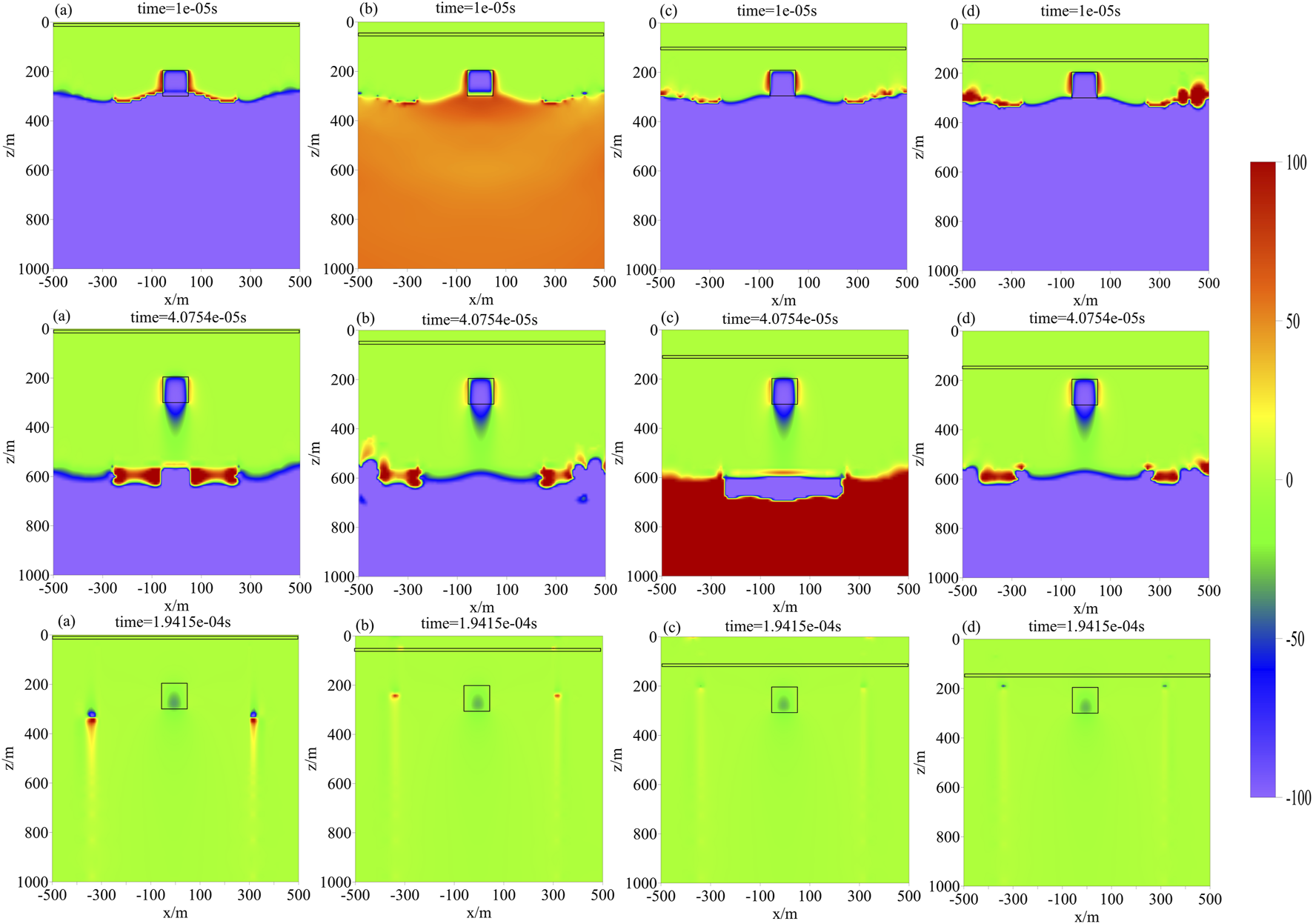
The distributions of the EMF across different times at the y = 0 cross-section were compared and analysed. The EMF distribution diagrams at 10⁻⁵ s, 4.0754 × 10⁻⁵ s, and 1.9415 × 10⁻⁴ s are shown in Figure 3. The rectangular boxes in the figure indicate the locations of the water-rich areas. At 10⁻⁵ s, owing to the proximity of the aquifer’s top interface to the transmitter loop (10 m deep), the secondary field decays slowly and spreads only slightly within the low-resistivity layer, leading to a concentration of secondary field extrema within the aquifer in Figure 3a, with a relatively small horizontal spread. At this time, the secondary field spread ranges of the other three models are similar. By 4.0754 × 10⁻⁵ s, the secondary field primarily spreads within the aquifer and above it. At 1.9415 × 10⁻⁴ s, the secondary field extrema of all the models appear in the shallow aquifer region. Influenced by the low resistivity of the water-rich areas, the secondary field values near the rectangular boxes exhibit significant changes.

Figure 3

Figure 3. Distribution of the EMF z component at 10⁻⁵ s,4.0754 × 10⁻⁵ s and 1.9415 × 10⁻⁴ s at different depths in the shallow aquifer: (a) h = 10 m, (b) h = 50 m, (c) h = 100 m, and (d) h = 150 m.

The EMF distributions at 9.2492 × 10⁻⁴ s and 4.4062 × 10⁻³ s are shown in Figure 4. At these times, the extremum of the secondary field is located in a water-rich area. At 4.4062 × 10⁻³ s, although the extremum of the secondary field in all the models is situated in the water-rich areas, there is no significant difference between the extremum and the surrounding secondary field.

Figure 4

Figure 4. Distribution of the EMF z component at 9.2492 × 10⁻⁴ s and 4.4062 × 10⁻³ s at different depths in the shallow aquifer: (a) h = 10 m, (b) h = 50 m (c) h = 100 m, and (d) h = 150 m.

3.1.2 Change rate of the induced electromagnetic field

Using the transient electromagnetic field of a uniform half-space as the background data and a model containing water-rich areas as the dataset for this study, we calculated the rate of change in the induced EMF and plotted the distribution of the rate of change in the induced EMF. The calculation formula is Equation 12:

$\mathit{R}\mathit{a}\mathit{t}\mathit{e}\mathit{o}\mathit{f}\mathit{C}\mathit{h}\mathit{a}\mathit{n}\mathit{g}\mathit{e}=\frac{{\mathit{E}\mathit{M}\mathit{F}}_{\mathit{S}}-{\mathit{E}\mathit{M}\mathit{F}}_{\mathit{B}}}{{\mathit{E}\mathit{M}\mathit{F}}_{\mathit{B}}}\times \mathbf{100}\%(12)$

where ${EMF}_S$ represents the simulated data and ${EMF}_B$ represents the background data.

A comparison and analysis of the rate of change in the EMF distribution at the y = 0 cross-section at different times was conducted. The distributions of the EMF rate of change at 10⁻⁵ s, 4.0754 × 10⁻⁵ s, and 1.9415 × 10⁻⁴ s are shown in Figure 5.

Figure 5

Figure 5. Distribution of the EMF change rates at 10⁻⁵ s,4.0754 × 10⁻⁵ s and 1.9415 × 10⁻⁴ s at different depths in the shallow aquifer: (a) h = 10 m, (b) h = 50 m, (c) h = 100 m, and (d) h = 150 m.

At 10⁻⁵ s, all the models display a “W” shaped interface at a longitudinal position of 300 m, with the concave part aligned with the position of the transmitter loop, indicating that this shape is caused by the loop. Above this interface, the rate of change in the EMF is almost zero, whereas below the interface, the rate of change in the EMF is relatively large. In all the models, the rate of change in the EMF within the water-rich areas is negative. At 4.0754 × 10⁻⁵ s, except for the region below 600 m longitudinally and near the water-rich zone, the EMF change rate is significantly greater, with the remaining regions showing nearly zero values. At 1.9415 × 10⁻⁴ s, all the models exhibit two bands of extreme values of the EMF change rate outside the transmitter loop, which decrease with increasing depth of the shallow aquifer, and the EMF change rates below the water-rich areas are greater than those above it.

The distributions of the rates of change in the EMF at 9.2492 × 10⁻⁴ s and 4.4062 × 10⁻³ s are shown in Figure 6. The maximum value of the EMF rate of change is located in the water-rich areas, with values above and below this area essentially being symmetrical. The distribution of the EMF rate of change does not significantly change with increasing depth of the shallow aquifer.

Figure 6

Figure 6. Distribution of the EMF change rates at 9.2492 × 10⁻⁴ s and 4.4062 × 10⁻³ s at different depths in the shallow aquifer: (a) h = 10 m, (b) h = 50 m (c) h = 100 m, and (d) h = 150 m.

The simulation results indicate that when the thickness of the shallow aquifer is held constant, variations in the depth of the shallow aquifer have no significant effect on the detection results of the deep water-rich areas.

3.1.3 Data characteristics of SUTEM

The simulation results indicate that when the thickness of the shallow aquifer is held constant, variations in the depth of the shallow aquifer do not significantly affect the detection outcomes of deep water-rich areas. The z-component EMF receiving points were established at the surface and 100 m, 300 m, and 500 m below the surface to analyse the characteristics of the SUTEM data under the influence of the shallow aquifer.

The EMF curves for the receiving points at different depths are shown in Figure 7. When the receiving points are at the surface and 100 m below the surface, the EMF curves exhibit significant differences in shape and value. However, when the receiving points are 300 m and 500 m below the surface, the EMF curves calculated by the model are very similar.

Figure 7

Figure 7. EMF curves of receiving points at different depths in the shallow aquifer: (a) d = 0 m, (b) d = −100 m, (c) d = −300 m, and (d) d = −500 m.

The EMF rates of the change curves for the receiving points at different depths are depicted in Figure 8. When the receiving point is at the surface, the EMF rate of change ranges from −0.15 to 0.3, with all the models exhibiting both positive and negative extrema. Considering the presence of industrial noise ranging from 3% to 5% in practical operations, the observed data can be considered not to contain electrical information from water-rich areas. When the receiving point is 100 m below the surface, the EMF rate of change is between −0.6 and 1.0, which is still below the noise interference level. However, when the receiving point is 300 m below the surface, the EMF rate of change ranges from −100 to 20, and the influence of the shallow aquifer with a constant thickness and varying depth on this curve is relatively small. When the receiving point is at 500 m below the surface, the data observed at the 500 m receiving point range from −20 to 1, exceeding the range of interfering noise.

Figure 8

Figure 8. EMF change rate curves of receiving points at different depths in the shallow aquifer (a) d = 0 m (b) d = −100 m (c) d = −300 m (d) d = −500 m.

3.2 Shallow aquifer with varying thicknesses at fixed depths

The thickness of the shallow aquifer was set to 20 m, 40 m, 60 m, and 80 m, with the centre point at a depth of 50 m.

3.2.1 Distribution characteristics of the electromagnetic field

An analysis of the distribution of the induced electromotive force (EMF) at the y = 0 cross-section at different times was conducted. The EMF distribution diagrams at 10⁻⁵ s, 4.0754 × 10⁻⁵ s, and 1.9415 × 10⁻⁴ s are shown in Figure 9. As observed from the figure, prior to 4.0754 × 10⁻⁵ s, the horizontal and longitudinal diffusion of the secondary field extrema is relatively slow because of the influence of the shallow aquifer, with the extrema mainly concentrated within the shallow aquifer. With increasing shallow aquifer thickness, the horizontal and longitudinal diffusion rates of the secondary field extrema decrease. At 1.9415 × 10⁻⁴ s, the secondary field extrema in all the models are located within the shallow aquifer, and as the thickness of the shallow aquifer increases, the rate at which the secondary field converges in the horizontal direction decreases.

Figure 9

Figure 9. Distribution of the EMF z component at 10⁻⁵ s, 4.0754 × 10⁻⁵ s and 1.9415 × 10⁻⁴ s at different shallow aquifer thicknesses: (a) d = 20 m, (b) d = 40 m, (c) d = 60 m, and (d) d = 80 m.

The EMF distributions at 9.2492 × 10⁻⁴ s and 4.4062 × 10⁻³ s are shown in Figure 10. In all the models, the extremum of the secondary field is within the shallow aquifer, but there is a distinct trend of diffusion towards the water-rich areas. At 4.4062 × 10⁻³ s, with increasing shallow aquifer thickness, the downwards diffusion speed of the secondary field extremum slows.

Figure 10

Figure 10. Distribution of the EMF z-component at 9.2492 × 10⁻⁴ s and 4.4062 × 10⁻³ s for different shallow aquifer thicknesses: (a) d = 20 m, (b) d = 40 m (c) d = 60 m, and (d) d = 80 m.

3.2.2 Change rate of the electromagnetic field

The distribution of the rate of change in the EMF at the y = 0 cross-section at different times was analysed by comparing the diagrams. At 10⁻⁵ s, 4.0754 × 10⁻⁵ s, and 1.9415 × 10⁻⁴ s, the EMF rate of change distribution is shown in Figure 11. At 10⁻⁵ s, all the models display a “W”-shaped interface in terms of the EMF rate of change, which increases with increasing thickness of the shallow aquifer. Above this interface, the rate of change is almost zero, whereas below the interface, the rate of change is significantly greater. Within the water-rich areas, the rate of change is relatively large and negative in all the models. By 4.0754 × 10⁻⁵ s, the “W” interface diminishes, with a significant rate of change only below the interface and near the water-rich areas. At 1.9415 × 10⁻⁴ s, the rate of change below the water-rich areas is greater than that above the water-rich areas, and the internal rate of change within the water-rich areas increases with increasing thickness of the shallow aquifer.

Figure 11

Figure 11. Distribution of the EMF change rates at 10⁻⁵ s, 4.0754 × 10⁻⁵ s and 1.9415 × 10⁻⁴ s for different shallow aquifer thicknesses: (a) d = 20 m, (b) d = 40 m (c) d = 60 m, and (d) d = 80 m.

The distributions of the rates of change in the EMF at 9.2492 × 10⁻⁴ s and 4.4062 × 10⁻³ s are depicted in Figure 12. The maximum values of the rate of change are located in the water-rich areas, with symmetrical values above and below. The thickness of the shallow aquifer significantly affects the distribution of the rate of change, indicating that when the longitudinal position of the shallow aquifer is fixed, variations in thickness have a substantial effect on the detection results of deep water areas.

Figure 12

Figure 12. Distribution of the EMF change rate at 9.2492 × 10⁻⁴ s and 4.4062 × 10⁻³ s for different shallow aquifer thicknesses: (a) d = 20 m, (b) d = 40 m (c) d = 60 m, and (d) d = 80 m.

3.2.3 Data characteristics of the SUTEM method

Z-component EMF receiving points were established at the surface and 100 m, 300 m, and 500 m below the surface.

The EMF curves for receiving points at different depths are shown in Figure 13. When the receiving point is at the surface, there are significant changes in both the morphology and the values of the induced electromotive force curves. When the receiving point is below the shallow aquifer, regardless of the depth, the morphology of the induced electromotive force curves is consistent, but the range of values varies significantly. The thicker the shallow aquifer is, the later the peak value of the data observed by the SUTEM method is, and the smaller the peak value is; however, it tends to approach a uniform semispace curve in the later period.

Figure 13

Figure 13. EMF curves of receiving points at different depths for different aquifer thicknesses: (a) d = 0 m, (b) d = −100 m (c) d = −300 m, and (d) d = −500 m.

The EMF rates of the change curves for the receiving points at different depths are shown in Figure 14. When the receiving point is at the surface, the range of the induced electromotive force (EMF) rate of change values is between −0.05 and 0.15, with all the models exhibiting both positive and negative extrema. Variations in the thickness of the shallow aquifer significantly affect the values of the rates of change curves. At a depth of 100 m below the surface, the rate of change ranges from −0.5 to 0.5, which is still less than the noise interference level. However, when the receiving point is 300 m below the surface, the induced EMF rate of change is between −100 and 10. At a depth of 500 m, which is equidistant from the surface observation point and the water-rich areas, the observed data range from −70 to 1, exceeding the range of interfering noise.

Figure 14

Figure 14. EMF change rate curves of receiving points at different depths for different aquifer thicknesses (a) d = 0 m (b) d = −100 m (c) d = −300 m (d) d = −500 m.

4 Practical application

4.1 Geophysical characteristics of the minefield

The study area is located in the 1102₂12 working face of Shi Cao Village, Ningdong Mining Area, Ningxia Hui Autonomous Region, China. The strata exposed in the mine field from old to new are as follows: the Upper Triassic System Shangtian Formation (T3S), the Jurassic System Middle Series Yan’an Formation (J2y), the Zhiluo Formation (J2z), the Anding Formation (J2a), the Palaeogene System (E), and the Quaternary System (Q), as shown in Table 1. There are two main aquifers above the first mining coal seam, namely, the Quaternary shallow aquifer and the Jurassic Middle Series Zhiluo Formation lower segment sandstone confined aquifer, among which the Jurassic Middle Series Zhiluo Formation sandstone aquifer is the direct water source for the first mining coal seam. The shallow aquifer in the Quaternary pores is distributed throughout the mine field, with groundwater recharge occurring mainly from atmospheric precipitation and discharge occurring mainly through evaporation. The Jurassic clastic rock fracture-pore confined aquifers mainly include the Jurassic Middle Series Anding to Zhiluo Formation aquifers and the Middle Series Yan’an Formation coal series strata aquifers. Based on the distribution of aquifers and hydrogeological characteristics, the aquifer with a significant impact on the mine field is the bottom sandstone aquifer segment of the Zhiluo Formation, which has poor cementation and strong water richness and is an average of 150 m away from the first mining coal seam. Other segments of aquifers are more compact, with less developed fractures and poor water richness, and are considered weak water-rich aquifers. Under normal strata combinations, there are regular patterns of physical properties both laterally and vertically. However, near structurally developed areas or water-rich areas, a large amount of mine water is present, which has good conductivity and breaks the inherent variation patterns of electrical properties both laterally and vertically. This change provides a physical basis for transient electromagnetic exploration on the basis of electrical properties.

Table 1

Table 1. Logging data of the mining area.

4.2 Construction scheme

The construction design is shown in Figure 15. With the transmitter loop set to 1000 × 500 m, the longer side was arranged along the strike of the working face, and the shorter side was arranged along the dip of the working face. The red points in the figure are the receiving points, with surface and underground receiving points forming two survey lines. The surface receiving survey line was arranged directly above the working face transportation tunnel on the surface, with a point spacing of 20 m. The underground receiving points were set up within the working face transportation tunnel, with a point spacing of 10 m.

Figure 15

Figure 15. Construction design.

Five experimental points were selected on each of the two survey lines for theoretical verification. The measured EMF data curves are shown in Figure 16, where (a) is the curve measured at the surface survey points, showing a smooth decay of the EMF over time, and (b) is the curve measured at the tunnel survey points, i.e., the survey points are underground, where the EMF shows an initial increase followed by a decrease over time, with a curve shape consistent with the theoretical research. Owing to various iron interferences and a smaller order of magnitude when received in the tunnel, the noise level of the underground reception is greater than that of the surface reception, leading to some oscillations in the curve shape in the later stages.

Figure 16

Figure 16. Measured data curves: (a) receiver at the surface and (b) receiver underground.

4.3 1D inversion interpretation

The inversion interpretation in this study uses the Occam smooth inversion, and the objective function of the inversion can be expressed by the following Equation 13 (Steven et al., 1987):

$\mathbf{\Phi }={\left(\mathbf{\Delta }\overrightarrow{\mathit{d}}-\mathit{J}\overrightarrow{\mathit{m}}\right)}^{\mathit{T}}\left(\mathbf{\Delta }\overrightarrow{\mathit{d}}-\mathit{J}\overrightarrow{\mathit{m}}\right)+\mathit{\lambda }{\left(\mathit{R}\overrightarrow{\mathit{m}}\right)}^{\mathit{T}}\left(\mathit{R}\overrightarrow{\mathit{m}}\right)(13)$

where $\Delta \overrightarrow{d}$ represents the difference between the measured data and the forward-modelled data; $\overrightarrow{m}$ represents the parameter vector of each node in the model; $J$ represents the Jacobian coefficient matrix; $\lambda$ represents the Lagrange multiplier; and $R$ represents the roughness matrix.

The model parameters can be modified by the following Equation 14:

$\mathbf{\Delta }\overrightarrow{\mathit{m}}={\left({\mathit{J}}^{\mathit{T}}\mathit{J}+\mathit{\lambda }{\mathit{R}}^{\mathit{T}}\mathit{R}\right)}^{-\mathbf{1}}\mathit{J}\mathbf{\Delta }\overrightarrow{\mathit{d}}(14)$

The root mean square error is commonly used to evaluate whether a forward model is close to the actual geological situation, and its expression is given by Equation 15:

$\mathit{R}\mathit{M}\mathit{S}=\sqrt{\frac{\mathbf{1}}{\mathit{N}}{\displaystyle \sum _{\mathit{i}=\mathbf{1}}^{\mathit{N}}}{\left(\frac{{\mathit{d}}_{\mathit{i}}-\mathit{f}{\left(\overrightarrow{\mathit{m}}\right)}_{\mathit{i}}}{{\mathit{d}}_{\mathit{i}}}\right)}^{\mathbf{2}}}\times \mathbf{100}\%(15)$

In the equation, $N$ is the number of observed data points, and $d_i$ is the ii-th observed data point.

Li conducted inversion studies on the simulation results of ground transient electromagnetic and underground transient electromagnetic methods, verifying the reliability and accuracy of the method (Li, 2022).

After the surface and underground data were obtained, one-dimensional inversions were performed separately. The number of inversion iterations and fitting errors for each point are shown in Figure 17. Due to the higher signal-to-noise ratio of the surface TEM data compared to SUTEM, the maximum number of iterations for the surface TEM inversion is set to 15, while for SUTEM, it is set to 30. As shown in Figure (a), the surface TEM inversion generally converges after 10 iterations, while SUTEM converges after 25 iterations. From Figure (b), it can be seen that the fitting errors for both methods are generally below 10%. However, due to some interference present in the SUTEM data, the fitting errors for a few points reach around 15%. Overall, the inversion results are credible.

Figure 17

Figure 17. Inversion iteration details: (a) The number of inversion iterations and (b) Data fitting error.

The one-dimensional inversion results were then combined into two-dimensional data to create resistivity profiles, as shown in Figures 18, 19. The black straight line in the figures indicates the location of the working face, and the red dashed line represents the position of the receiving points.

Figure 18

Figure 18. Surface transient electromagnetic method detection results.

Figure 19

Figure 19. Surface-to-underground transient electromagnetic method detection results.

Figure 18 shows the results of the surface transient electromagnetic method. The figure shows that the data are affected by the shielding of the shallow Quaternary aquifer, resulting in relatively high resistivity values obtained in the early stages. This makes accurate identification of the water-rich areas in the shallow Quaternary and the thick sandstone layer of the Zhiluo Formation in the Jurassic Middle Series difficult. The resistivity values show a high-low variation trend from top to bottom.

Figure 19 shows the results of the SUTEM method. The resistivity tends to be high-low-high-low-high in the vertical direction. There is also a relatively continuous lateral change in the shallow part, and the lateral resolution is greater in the deep part, which is unaffected by the shallow aquifer. This finding indicates that under the shielding of shallow aquifers, SUTEM technology is more sensitive to deep aquifers and can better reflect the electrical information of deep layers. The results of the SUTEM analysis correlate well with the hydrogeological conditions and logging data of the mine, providing a reference for subsequent water exploration and drainage work in the coal mine.

5 Discussion

To achieve the detection of deep aquifers under the influence of shallow low-resistivity shielding layers, traditional surface electrical exploration methods are significantly affected by these low-resistivity layers and are unable to effectively detect deep aquifers. Although electrical methods directly employed in tunnels can ignore the shallow low-resistivity layers and achieve direct detection, their detection range and accuracy are limited due to the restricted tunnel space and limited working current (Su et al., 2022; Shi et al., 2019). The SUTEM overcomes these limitations by receiving secondary field signals generated by deep aquifers without interference from shallow low-resistivity layers, thus obtaining more geological information about the aquifers (Chang et al., 2019b).

This study takes the typical geological structure of the Ningdong Mining Area as the research object. Numerical simulations and field applications of both surface TEM and SUTEM show that while surface TEM cannot overcome the low-resistivity shielding, it still possesses some capability for vertical positioning. In contrast, SUTEM successfully penetrates the shallow low-resistivity layers to obtain information about deep aquifers. Compared to traditional surface TEM, SUTEM can more clearly identify changes in deep geological structures. Although SUTEM performs well in deep detection, its vertical resolution for shallow low-resistivity layers is relatively low, and it should be combined with traditional methods for shallow exploration.

Compared with existing studies, this research not only theoretically analyzes the electromagnetic field distribution characteristics of SUTEM but also validates its applicability in complex geological conditions through field applications, overcoming the limitations of traditional methods. Moreover, this study provides a theoretical basis for optimizing detection parameters in practical applications by analyzing the effects of the thickness and burial depth of shallow aquifers on SUTEM detection results.

6 Conclusion

This study, which was grounded in actual geological conditions, employed numerical simulations to investigate the distribution characteristics of transient electromagnetic fields and the data characteristics of the SUTEM method under the influence of shallow aquifers of varying depths and thicknesses. The main conclusions are as follows:

(1) When the shallow aquifer thickness is fixed, changes in depth have no significant effect on the ability of SUTEM to detect deep aquifers or water-rich areas but significantly affect surface and shallow subsurface receivers, indicating that SUTEM has limited vertical resolution for shallow low-resistivity layers.

(2) When the depth of a shallow aquifer is fixed and its thickness varies, it significantly affects the detection of deep aquifers or water-rich areas by TEM, with SUTEM being more sensitive to the thickness of shallow low-resistivity layers.

(3) Simulations under the shielding of shallow aquifers reveal that SUTEM technology has a stronger detection capability for water-rich areas than do surface transient electromagnetic methods.

(4) Field data from the Shicao Village coal mine in the Ningdong mining area show that, influenced by shallow aquifers, SUTEM receives more geological information from deep aquifers, with resistivity exhibiting a high-low-high-low-high variation trend longitudinally, whereas surface transient electromagnetic results show a transition from high to low resistivity, which is consistent with theoretical outcomes.

Data availability statement

The raw data supporting the conclusions of this article will be made available by the authors, without undue reservation.

Author contributions

ML: Writing–original draft, Writing–review and editing. ZD: Writing–original draft, Writing–review and editing. ZJ: Writing–original draft, Writing–review and editing. JY: Writing–original draft, Writing–review and editing. LX: Writing–original draft, Writing–review and editing.

Funding

The author(s) declare that no financial support was received for the research and/or publication of this article.

Conflict of interest

The authors declare that the research was conducted in the absence of any commercial or financial relationships that could be construed as a potential conflict of interest.

Generative AI statement

The author(s) declare that no Generative AI was used in the creation of this manuscript.

Publisher’s note

All claims expressed in this article are solely those of the authors and do not necessarily represent those of their affiliated organizations, or those of the publisher, the editors and the reviewers. Any product that may be evaluated in this article, or claim that may be made by its manufacturer, is not guaranteed or endorsed by the publisher.

References

Anomohanran, O., and Orhiunu, M. E. (2018). Assessment of groundwater occurrence in Olomoro, Nigeria using borehole logging and electrical resistivity methods. Arabian J. Geosciences 11 (9), 219. doi:10.1007/s12517-018-3582-7

CrossRef Full Text | Google Scholar

Chang, J. H., Su, B. Y., Malekian, R., and Xing, X. J. (2020). Detection of water-filled mining goaf using mining transient electromagnetic method. IEEE Trans. Industrial Inf. 16 (5), 2977–2984. doi:10.1109/TII.2019.2901856

CrossRef Full Text | Google Scholar

Chang, J. H., Xue, G. Q., and Malekian, R. (2019a). A comparison of surface-to-coal mine roadway TEM and surface TEM responses to water-enriched bodies. IEEE ACCESS 7, 167320–167328. doi:10.1109/ACCESS.2019.2953844

CrossRef Full Text | Google Scholar

Chang, J. H., Yu, J. C., Li, J. J., Xue, G. Q., Malekian, R., and Su, B. Y. (2019b). Diffusion law of whole-space transient electromagnetic field generated by the underground magnetic source and its application. IEEE Access 7, 63415–63425. doi:10.1109/ACCESS.2019.2916767

CrossRef Full Text | Google Scholar

Cheng, J. L., Xue, J. J., Zhou, J., Dong, Y., and Wen, L. F. (2020). 2.5-D inversion of advanced detection transient electromagnetic method in full space. IEEE Access 8, 4972–4979. doi:10.1109/ACCESS.2019.2962963

CrossRef Full Text | Google Scholar

Delima, O. A. L. (1993). Geophysical evaluation of sandstone aquifers in the Recôncavo-Tucano Basin, Bahia—Brazil. Geophysics 58 (11), 1689–1702. doi:10.1190/1.1443384

CrossRef Full Text | Google Scholar

Hasan, M., Shang, Y. J., and Jin, W. J. (2018). Delineation of weathered/fracture zones for aquifer potential using an integrated geophysical approach: a case study from South China. J. Appl. Geophys. 157, 47–60. doi:10.1016/j.jappgeo.2018.06.017

CrossRef Full Text | Google Scholar

Jiang, Z. H., Liu, L., Liu, S. C., and Yue, J. H. (2020). Response characteristics of water-bearing goafs for surface-to-underground transient electromagnetic method. J. Environ. Eng. Geophys. 24 (4), 557–567. doi:10.2113/JEEG24.4.557

CrossRef Full Text | Google Scholar

Jiang, Z. H., Liu, L. B., Liu, S. C., and Yue, J. H. (2019). Surface-to-Underground transient electromagnetic detection of water-bearing goaves. IEEE Trans. Geoscience Remote Sens. 57 (8), 5303–5318. doi:10.1109/TGRS.2019.2898904

CrossRef Full Text | Google Scholar

Jr, J. F., Tandy, T., Halihan, T., Ross, R., Beak, D., Neill, R., et al. (2022). Electrical resistivity imaging of an enhanced aquifer recharge site. J. Geophys. Eng. 19 (5), 1095–1110. doi:10.1093/jge/gxac073

CrossRef Full Text | Google Scholar

Kumar, D. (2012). Efficacy of electrical resistivity tomography technique in mapping shallow subsurface anomaly. J. Geol. Soc. India 80 (3), 304–307. doi:10.1007/s12594-012-0148-2

CrossRef Full Text | Google Scholar

Li, M. F. (2022). Joint inversion interpretation of surface and surface-to-underground electromagnetic method. Xuzhou, Jiangsu, China: China University of Mining and Technology. [Doctoral dissertation].

Google Scholar

Li, M. F., Jiang, Z. H., Liu, L., Liu, S. C., Chen, S. B., and Tong, X. R. (2024). Electromagnetic field distribution and data characteristics of SUTEM of multilayer aquifers. Appl. Sciences-Basel 14 (20), 9358. doi:10.3390/app14209358

CrossRef Full Text | Google Scholar

Lin, W. X. (2022). Monitoring bed separation water using Surface-to-Underground Transient Electromagnetic Method. [Master's thesis]. Xuzhou, Jiangsu, China: China University of Mining and Technology.

Google Scholar

Manrique, I. I., Caterina, D., Nguyen, F., and Hermans, T. (2023). Quantitative interpretation of geoelectric inverted data with a robust probabilistic approach. Geophysics 88 (3), B151–B166. doi:10.1190/GEO2022-0133.1

CrossRef Full Text | Google Scholar

Nikam, R., Kumar, G. P., Prasad, A. D., Chaube, H., and Chopra, S. (2023). Delineation of paleochannel and groundwater resources in the Khari river basin, Kachchh using transient electromagnetics. J. Geol. Soc. India 99 (2), 239–246. doi:10.1007/s12594-023-2291-3

CrossRef Full Text | Google Scholar

Shi, L. Q., Wang, Y., Qiu, M., Gao, M. F., and Zhai, P. H. (2019). Application of three-dimensional high-density resistivity method in roof water advanced detection during working stope mining. Arabian J. Geosciences 12 (15), 464. doi:10.1007/s12517-019-4586-7

CrossRef Full Text | Google Scholar

Steven, C. C., Robert, L. P., and Catherine, G. C. (1987). Occam’s inversion: a practical algorithm for generating smooth models from electromagnetic sounding data. Geophysics 52 (3), 267–462. doi:10.1190/1.1442303

CrossRef Full Text | Google Scholar

Su, M. X., Cheng, K., Li, H. Y., Xue, Y. G., Wang, P., Ma, X. Y., et al. (2022). Comprehensive investigation of water-conducting channels in near-sea limestone mines using microtremor survey, electrical resistivity tomography, and tracer tests: a case study in Beihai City, China. Bull. Eng. Geol. Environ. 81 (5), 184. doi:10.1007/s10064-022-02684-1

CrossRef Full Text | Google Scholar

Sun, H. F., Li, X., Li, S. C., Qi, Z. P., Wang, W. P., Su, M. X., et al. (2013). Three-dimensional FDTD modeling of TEM excited by a loop source considering ramp time. Chin. J. Geophys. 56 (3), 1049–1064. doi:10.6038/cjg20130333

CrossRef Full Text | Google Scholar

Wang, T., and Hohmann, G. W. (1993). A finite-difference time-domain Solution for three-dimensional electromagnetic modeling. Geophysics 58 (6), 797–809. doi:10.1190/1.1443465

CrossRef Full Text | Google Scholar

Wang, Y. Z., Yu, J. C., Feng, X. H., Ma, L., Gao, Q. H., Su, B. Y., et al. (2021). A case study of direct current resistivity method for disaster water source detection in coal mining. Elektron. Ir. Elektrotechnika. 27 (4), 41–48. doi:10.5755/j02.eie.29090

CrossRef Full Text | Google Scholar

Wu, R. X., Hu, Z. A., and Hu, X. W. (2020). Principle of using borehole electrode current method to monitor the overburden stratum failure after coal seam mining and its application. J. Appl. Geophys. 179, 104111. doi:10.1016/j.jappgeo.2020.104111

CrossRef Full Text | Google Scholar

Yang, Y. (2022). Study on vector-intersecting interpretation method of surface-to-underground transient electromagnetic data. [Master's thesis]. Xuzhou, Jiangsu, China: China University of Mining and Technology.

Google Scholar

Yee, K. S. (1966). Numerical solution of initial boundary problems involving Maxwell's equations in isotropic media. IEEE Trans. 14 (3), 302–307. doi:10.1109/TAP.1966.1138693

CrossRef Full Text | Google Scholar

Yu, J. C., Malekian, R., Chang, J. H., and Su, B. Y. (2017). Modeling of whole-space transient electromagnetic responses based on FDTD and its application in the mining industry. IEEE 13 (6), 2974–2982. doi:10.1109/TII.2017.2752230

CrossRef Full Text | Google Scholar