An approach for teleseismic location by automatically matching depth phase

To deal with the low efficiency problem of accurate teleseismic hypocenter location, this paper proposes a fully automatic approach by integrating the advantages of Seismic-Scanning based on Navigated Automatic Phase-picking, which can automatically detect and locate seismic events from continuous waveforms, and the Depth-Scanning Algorithm, which can determine the precise focal depth of local and regional earthquakes by matching depth phases. This approach, named TeleHypo, automatically searches and downloads seismic station data from the Data Management Center of the Incorporated Research Institutions for Seismology according to the original time and centroid location of teleseismic earthquakes reported by the Global Centroid-Moment-Tensor Project. Then, the direct wave was automatic extracted to construct depth-phase templates. All possible depth phases after the direct phase are obtained through a match-filtering method. Finally, high-precision hypocenter depth is determined according to the relationship between the travel time differences of the direct waves and depth phases. TeleHypo can obtain high-precision teleseismic hypocenter parameters automatically through the above process. This approach has been successfully applied to 55 teleseismic events occurred in different global seismogenic regions. It can be used to establish high-quality teleseismic catalogue and depth-phase database.

1 Introduction

As an important seismic source parameter, the hypocenter is not only helpful for the analysis of the initial stress state and instability position of the seismogenic region, but also can jointly explain the rupture direction and length with the centroid location (see Figure 1; Smith and Ekström, 1997). It plays a crucial role to focal mechanism inversion and real-time earthquake warning (Shelly et al., 2007; He and Ni, 2017). However, the local geological structure of many remote areas is complex. When seismic network in these areas is sparse or unevenly distributed, there is often a lack of reliable adjacent stations to accurately and automatically locate the hypocenter (Tan et al., 2019; Yuan et al., 2020).

Figure 1

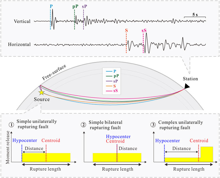
Figure 1. Hypocenter and centroid can jointly reveal the direction and length of earthquake rupture (modified from Smith and Ekström (1997).

In the absence of a fine near-field velocity model and station data, the hypocenter of an earthquake of large magnitude can be determined using global teleseismic data by travel-time location method. Many authorities (e.g., United States Geological Survey, International Seismological Centre) use this mean for earthquake rapid report and generation of earthquake catalogue. However, with the increase of epicentral distance, the first-arrival travel time becomes insensitive to source depth. This would lead to a large error in the hypocenter location. That will further make it be unable to reveal the character of rupturing fault by using hypocenter location and the centroid location obtained by the Global Centroid-Moment-Tensor (GCMT) inversion method (see the bottom panel of Figure 1; Dziewonski and Anderson, 1981; Smith and Ekström, 1997).

The travel time difference between direct wave and the depth phases related to the free surface can be used to constrain the hypocenter depth with high accuracy (Kao and Chen, 1991; He et al., 2019; Yuan et al., 2020). However, current methods of improving the location accuracy by using the depth phase of teleseismic earthquakes are still limited by the accuracy and efficiency of depth-phase identification. For example, the International Seismological Centre (ISC) requires manual intervention in the depth-phase confirmation process, which usually takes 2 years to update their catalogue (Engdahl et al., 2020).

To improve the efficiency of depth-phase identification and location, Heyburn and Bowers (2008) proposed a semi-automatic statistical method to identify pP and sP. However, this method may treat the converted wave (S to P) from the Moho surface below the station as pP or sP and consequently results in wrong location. Letort et al. (2015) developed a focal depth location technology that can automatically identify pP and sP, but this method cannot evaluate the depths of earthquakes for the situations that produce only pP or only sP phases. For precise identification of pP, Florez and Prieto (2017) used the station array to carry out velocity spectrum analysis to obtain the accurate travel time difference of pP and P. However, this method assumes that the depth seismic phase identified is always pP, which is often unfortunately not true in practice. To use the travel times of the three depth phases, pP, sP and sS, to solve the hypocenter depth at the same time, Craig (2019) proposed an automated stacking routine using a globally distributed array. However, this semiautomatic technology required analyst input in refining appropriate frequency bands and wavelet window lengths to use, and in inspecting results to check for robustness. To automatically obtain a complete earthquake catalogue, Tan et al. (2019) proposed a fully automatic location method, called Seismicity-Scanning based on Navigated Automatic Phase-picking (S-SNAP). It is successfully applied to the Ridgecrest earthquake sequences in California, United States. But the hypocenter depth of S-SNAP in the case of large epicentral distance carries large uncertainty. To improve focal depth location precision of local and regional earthquakes, Yuan et al. (2020) proposed the Depth-Scanning Algorithm (DSA), which can automatically search all possible depth phases after direct phase to obtain precise hypocenter depth. DSA has been successfully applied to the events from different tectonic settings in Oklahoma, South Carolina, and California. The limitation of DSA is only applicable to constrain the depth location of local/regional earthquake. It also lacks the ability to relocate the epicenter and origin time. If the advantages of S-SNAP and DSA are integrated, a fully automatic precise location method can be developed to suit teleseismic events. In addition, the new method can also avoid the process of artificial intervention in depth-phase identification.

To this end, we combine S-SNAP and DSA to form a new approach, named TeleHypo, for teleseismic hypocenter location.

2 Methods

TeleHypo is complished by three steps: Teleseismic data preprocessing, preliminary hypocenter determination, and precise location of hypocenter depth, as introduced below.

2.1 Teleseismic data preprocessing

To obtain station data with a high signal-to-noise ratio (S/N) and avoid dominant location deviation caused by over-dense local network (such as USArray in the United States), a series of specific measures are adopted to preprocess the data:

a) According to the time and centroid location of the teleseismic event reported by GCMT, we select the waveform data of all available stations using a time window within 30 min before and after, separately, the original time and within the epicenter range from 30° to 90°. Then the mean value, linear trend, and instrument response are removed from the waveform data. After that, a 0.25–5.00 Hz band-pass filtering is carried out.

b) Three-component waveforms are rotated to vertical (Z), radial (R), and tangential (T) components. The Z and T components are used for the subsequent locating process of TeleHypo due to the interferences of pS, sea water layer multiple (i.e., pwP), and other seismic phases that often exist in the R component (Craig, 2019). Considering that the amplitudes of pS and pwP within the epicentral distance range of 30°–90° are usually weak, there are no PKP or its branch phases within this range, and SKS and its branch phases usually appear at stations with an epicenter distance of 70° or more. Therefore, three commonly used depth phases (i.e., pP, sP, and sS) with strong amplitudes within this range are used for constraining the depth of the seismic source by TeleHypo.

c) Travel times of the direct waves are calculated using AK135 velocity model (Kennett et al., 1995) according to the centroid and station position. Signal to noise ratio (S/N) is defined as TW2/TW1, where TW1 is the recording from the time window between 40 s and 10 s before the P arrival (Marked purple in Figure 3B), and TW2 is defined as the recording from the 30 s width window directly after the P arrival (Marked green in Figure 3B). The 10 s time-interval before the P arrival is to avoid the direct wave’s involvement in TW1 due to velocity model errors. To obtain reliable results, only high-quality data of S/N$\ge$3 are selected for use. These selected high S/N station data will be used for the following hypocenter determination.

2.2 Preliminary hypocenter determination

The technique used for preliminary hypocenter location of TeleHypo is modified from S-SNAP published by Tan et al. (2019). S-SNAP can automatically detect seismic events from continuous waveforms and determine the original time, magnitude, and spatial location of earthquakes. In the locating process, S-SNAP first scans the continuous waveform using the SSA method (Kao and Shan, 2004) to obtain the possible onset time and location of the event; Then, waveform segments containing the direct waves are intercepted and used to automatically pick up the first arrival time of P and S through the kurtosis function (Baillard et al., 2014). These first arrival times are used to improve the location accuracy of the original time and spatial location of the earthquake via the MAXI method (Font et al., 2004). Finally, the results obtained by MAXI are used as a preliminary solution.

It must be pointed out that there are two reasons for using S-SNAP in this paper. Firstly, we need to use S-SNAP to relocate the epicenter based on GCMT. Secondly, this will provide a teleseismic relocation algorithm to more researchers, facilitating their own location works and improving the convenience of scientific research.

It should also be pointed out that for earthquakes of large magnitudes, the centroid and hypocenter may not necessarily be at the same spatial location (see Figure 1). TeleHypo uses S-SNAP to determine the hypocenter (i.e., the starting point of the source rupture), which may not be approximated by the centroid provided by GCMT. In addition, for the station data with an epicenter distance range of 30°–90°, S-SNAP locates the epicenter mainly through the plane wave information of each station. Therefore, we believe that the epicenter location of S-SNAP is robust, which also indicates that when the station is far away from the hypocenter of the earthquake, the accuracy of depth obtained by S-SNAP is often poor because the ray path of direct phase is insensitive to source depth. To overcome this defect, we conjunct the DSA method of Yuan et al. (2020) to improve the hypocenter depth location for teleseismic events.

2.3 Precise location of hypocenter depth

Depth-phase templates are calculated by transforming the direct phase obtained in the first step (Section 2.1) into frequency domain, applying phase shift to the direct phase spectra, and transforming back into the time domain (as shown in Figure 2). With these templates, we carry out matching filter (Shelly et al., 2007) to find out all possible depth phases in the Z/R/T waveforms. Then the arrival time difference between each possible depth phase and direct wave is calculated and treated as observed data. These observed data will be compared with the theoretical ones, which is calculated by using the widely used TauP program (Krischer et al., 2015) with a series of given hypothetical source depths.

Figure 2

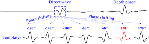
Figure 2. Automatic generation of depth phase templates by applying a series of phase shifting, from −180° to 180°, with an interval of 10°, to direct phase (dashed box). The depth phase (text in red in the top waveform) is successfully matched by the template (the waveform segment in red) generated by the direct phase after phase shifting of 120°.

For each presumed source depth, we count the number of matches and calculate the differential time residuals between the arrival times of the predicted depth phases and the observed with respect to the direct phase. This process is repeated for a range of assumed source depths at an increment of 1 km. Then, the same process is repeated for all available stations. After all stations are scanned for possible depth phases, we sum the total number of phase matches for each assumed focal depth and calculate the corresponding differential arrival time residual. Focal depths with the number of matches exceeding $\ge 90\%$ of the largest number of matches are taken as preliminary candidates. Among them, the hypothetical depth with the smallest total of travel time difference among these candidates is selected as the high-precision hypocenter depth solution. Finally, the theoretical depth phases (i.e., pP, sP, and sS) calculated by Taup corresponding to this depth solution are used to calibrate the observed depth-phase candidates that meet the matching conditions.

3 Application to teleseismic data

3.1 The 4 March 2010 Mw 6.3 Chile earthquake

The Mw 6.3 Chile earthquake occurred on 4 March 2010 at 22:39:29, at 22.360°N and 68.690°W, with a centroid depth of 118.7 km (the red star in Figure 3A).

Figure 3

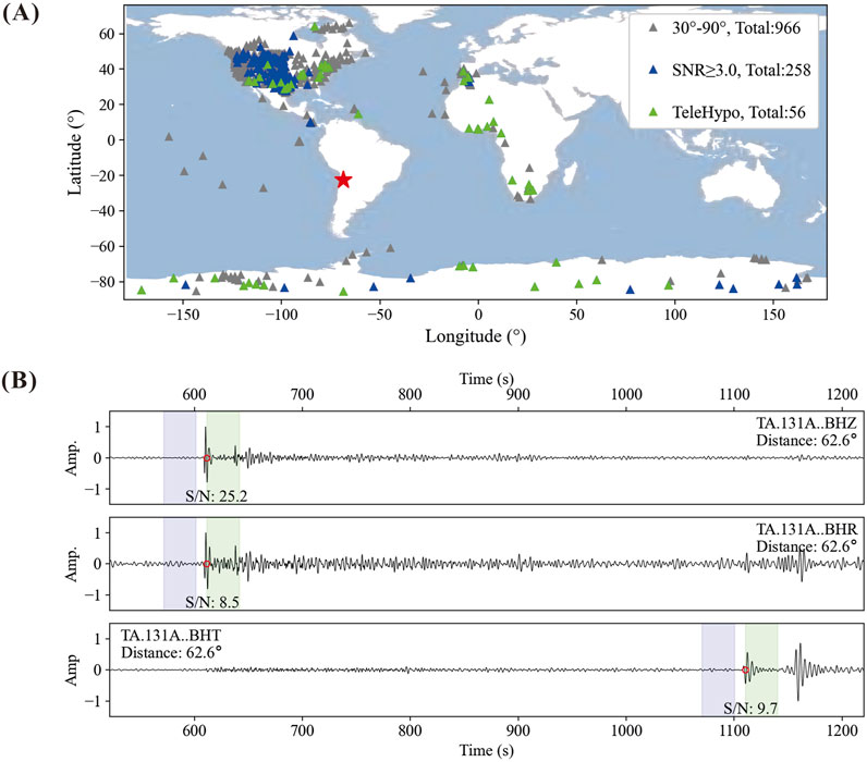
Figure 3. The Chile earthquake (4 March 2010, 22:39:29, Mw 6.3, the red star in (A)), all available stations (the gray, blue and green triangles in (A)), stations with S/N$\ge$3 (the blue triangles in (A)), and high S/N stations (the green triangles in (A)) used by TeleHypo. (B) shows the three-component waveform of station TA.131A with an epicenter distance of 62.6°. The S/N is defined as the ratio of the maximum absolute amplitude values of the waveforms shown in the purple and green windows. The red opened circle is the theoretical travel time of direct wave calculated based on GCMT and AK135 velocity model.

There are 966 stations (the gray, blue, and green triangles in Figure 3A) within the range of 30°–90° epicentral distance, and the 60 min width time window beginning 30 min before and ending 30 min after the earthquake original time provided by the GCMT. The waveform data of these stations were processed using the first step of TeleHypo. We kept the wavefield information within the frequency band of 0.25–5.0 Hz (Figure 3B). Next, the theoretical travel times of direct waves (P and S) were calculated according to the GCMT centroid and the position of each station (red circle in Figure 3B). The ratio of the largest absolute amplitudes of the waveforms (the purple and green windows in Figure 3B) is defined as the signal-to-noise ratio (S/N). To avoid systematic biases caused by nonuniform distribution of station-density, we divided stations into 36 regions at an azimuth interval of 10°, and selected only the top 5 high S/N stations from each region. We finally selected 56 high S/N stations (the green triangle in Figure 3A) for the following precise hypocenter location.

TeleHypo uses the centroid position of GCMT as a reference to search for hypocenter location. The search range for the hypocenter location is 22.36$\pm$ 1°N and 68.69$\pm$ 1°W, with a latitude and longitude interval of 0.1°. The depth scanning range is within the centroid depth $\pm$50 km, with a depth interval of 1 km. We extracted waveform segments from each station using a sliding window of 50 s with a step size of 1 s. The sum (called E) of squares of the waveform amplitudes within the sliding time window is calculated as a function of scanning time step (Figure 4A). Then, we searched for the P- and S-wave arrival times for possible events with E exceeding threshold of 1 (the red line in Figure 4A). Using the MAXI method (Font et al., 2004), the earthquake origin time of 4 March 2010, 22:39:26 and hypocenter location of 22.060°N, 68.465°W were located (the white circle in the upper right panel of Figure 4B). Finally, depth phases were matched with the templates at each assumed depth for each station below the hypocenter location. The scanning depth at 111 km with the highest number of successful matches is token as the hypocenter depth (the vertical dashed line in Figure 4C), along with the corresponding matched depth phases (Figure 4D).

Figure 4

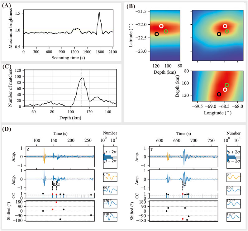
Figure 4. Stacked energy as a function of scanning time step obtained by TeleHypo (the black line in (A)) and threshold value used to determine possible earthquake events (red line in (A)). (B) shows the location solutions of TeleHypo (the white circles), ISC-EHB (the green circles) and GCMT (the black circles). (C) shows the hypocenter depth (vertical dotted line) obtained by TeleHypo through depth phase constraint. (D) shows the depth phase matching on the Z and T components of station TA.131A.

Comparing the solution obtained by TeleHypo (22.060°N, 68.465°W, 111 km, see the white circle in Figure 4B) with that of ISC-EHB (22.261°N, 68.400°W, 103.4 km, see the green circle in Figure 4B), we found that the two methods differ by about 0.201°N, 0.065°W in the epicenter location and 7.6 km in the source depth. The good agreement between the TeleHypo and ISC-EHB in this application example demonstrates the practicality of our method.

3.2 Teleseismic events from different global seismogenic regions

To further test the practicality of TeleHypo for global teleseismic events, we applied TeleHypo to 54 moderate-to-strong teleseismic events occurring in different seismogenic regions of the world (the open circles in Figure 5A). The source parameters of these earthquakes were obtained from the GCMT earthquake catalog, with magnitudes ranging from Mw 5.5 to 7.5, and centroid depths ranging from 20 to 200 km.

Figure 5

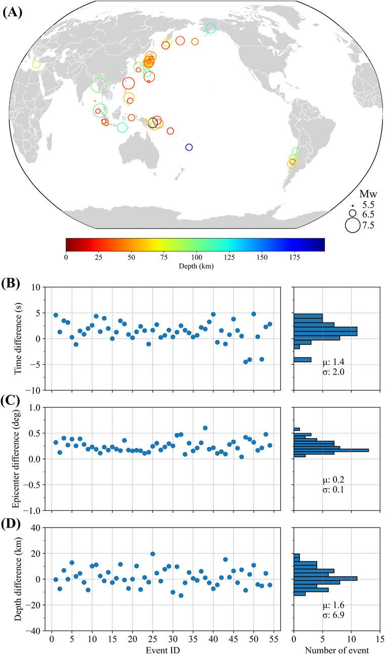
Figure 5. The map of 54 global teleseismic events (A). (B–D) respectively, show the differences of original time, epicenter distance, and depth between TeleHypo and ISC-EHB. $\mu$ and $\sigma$ represent the mean and standard deviation respectively.

We used TeleHypo with the same parameters as the previous example of the Chile earthquake to locate the hypocenters of these teleseismic events. The location results obtained by TeleHypo are compared with those of the ISC-EHB (see details in Supplementary Table S1 in the appendix). It is showed that the differences of the original time (Figure 5B), epicenter distance (Figure 5C), and hypocenter depth (Figure 5D) between the two methods were 1.4 $\pm$ 2.0 s, 0.2 $\pm$ 0.1°, and 1.6 $\pm$ 6.9 km, respectively. The depth distributions obtained by ISC-EHB (The blue dotted line in Figure 6) and TeleHypo (The orange dotted line in Figure 6) has good agreement. These high precision results demonstrate that TeleHypo has good applicability to teleseismic events occurring in different regions of the world.

Figure 6

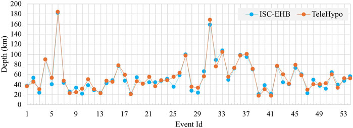
Figure 6. Depth distributions between ISC-EHB (The blue dotted line) and TeleHypo (The orange dotted line).

4 Discussion

4.1 Impact of the number of stations

To test the influence of the number of stations used on the location accuracy of TeleHypo, we conducted experiments on the Chile earthquake case in Section 3.1 by using 1, 3, and 5 stations with high S/N, separately, selected from each azimuthal area. We also conducted similar experiments on 54 global earthquakes in Section 3.2. The difference of origin time, epicentral location, and hypocenter depth between TeleHypo and ISC-EHB catalog were calculated. The statistical results showed that when we use only one station from each azimuthal area, the difference in origin time, epicentral location, and hypocenter depth are 1.1 $\pm$ 1.6 s, 0.2 $\pm$ 0.1°, and 5.8 $\pm$ 24.8 km, respectively (the right column of Figure 7). When three stations from each azimuthal area are used, the differences are 1.6 $\pm$ 1.6 s, 0.3 $\pm$ 0.1°, and 4.7 $\pm$ 9.0 km, respectively (the middle column of Figure 7). When the number of stations in each azimuthal sector reached 5, the differences are 1.5 $\pm$ 1.7 s, 0.2 $\pm$ 0.1°, and 2.0 $\pm$ 6.6 km, respectively (the left column of Figure 7). It indicates that using number of 5 stations with high S/N selected from each azimuthal area is suitable for TeleHypo.

Figure 7

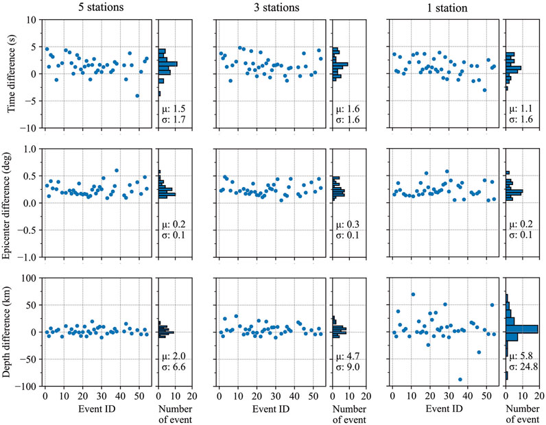
Figure 7. Hypocenter parameters located by TeleHypo using 5 (left column), 3 (middle column) and 1 (right column) high-quality stations, separately, from each azimuth area. The three rows of panels from top to bottom are the original time, epicenter distance, and hypocenter depth differences between TeleHypo and ISC-EHB, respectively. $\mu$ and $\sigma$ represent the mean and standard deviation, respectively.

It should be pointed out that the selection of stations for TeleHypo is centered around the epicenter of CGMT. The coverage is divided into 36 regions at intervals of 10° in azimuth. A maximum of 5 high S/N stations are selected from each region. Since the number of high S/N stations in some azimuthal areas can be less than 5, the total number of high S/N stations in all azimuth areas is usually less than 180, which also means that the number of depth phases with high quality will be less than 180. Section 4.4 below presents the statistical results of the number of high S/N stations and depth phases available for each of the five shallow earthquakes (see Figure 10). It indicates that TeleHypo does not necessarily need to use 180 depth phases to obtain accurate source depths.

4.2 The impact of velocity model

TeleHypo needs to use velocity model to calculate the travel times of direct waves and depth phases during location. To test the influence of different velocity models on the location of TeleHypo, we selected the IASP91 (Kennett and Engdahl, 1991) (see their Table 2) and AK135 (Kennett et al., 1995) (see their Table 3) velocity models for testing. The P-wave velocities of these two velocity models are almost the same. However, there are slight differences in their S-wave velocities, especially in the velocities above mantle where the S-wave velocity difference can reach 0.1 km/s. This difference can affect the travel time of S-waves and their associated free surface reflection phases (such as sP and sS), resulting in source location differences using these two velocity models.

We used the IASP91 velocity model to reconducted the locating experiments in Section 3.2. Other experimental parameters are the same as Section 3.2. When IASP91 is used, the differences between TeleHypo and ISC-EHB in origin time, epicentral location, and hypocenter depth are 1.8 $\pm$ 2.1 s, 0.2 $\pm$ 0.1°, and 0.8 $\pm$ 7.6 km, respectively (the left column of Figure 8). When AK135 is used, those differences are 1.4 $\pm$ 2.0 s, 0.2 $\pm$ 0.1°, and 1.6 $\pm$ 6.9 km, respectively (the right column of Figure 8). It suggests that IASP91 is more suitable for TeleHypo to locate the hypocenter depth.

Figure 8

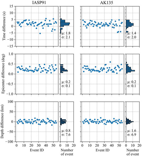
Figure 8. Hypocenter parameters located by TeleHypo using the IASP91 (left column) and AK135 (right column) velocity models. The layout is the same as Figure 7.

4.3 Seismic phase database

In addition to providing hypocenter parameters, TeleHypo can also provide the arrival times and be used to extract waveform of direct waves and depth phases (as shown in Figure 9), which is useful for building database for direct waves and depth phases of global earthquakes. The direct waves (P and S) and depth phases (pP, sP, and sS) for all teleseismic events in this paper were automatically picked by TeleHypo. There were, in total, 1245 P, 1245 S, 566 pP, 453 sP, and 456 sS phases. Since artificial intelligence nowadays still depends on good training data, TeleHypo can be used to provide a large number of training dataset and labels for artificial intelligence in teleseismic phase identification.

Figure 9

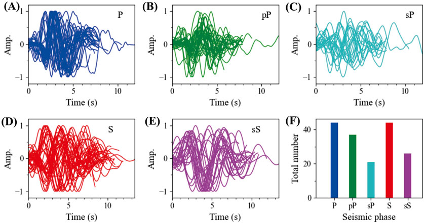
Figure 9. The direct waves (A,D), depth phases (B,C,E), and the number of these seismic phases (F) picked by TeleHypo from the high S/N stations of the Chile earthquake in Section 3.1.

4.4 Applicability of TeleHypo to shallow earthquakes

Among the 55 teleseismic events used in this paper (see the Supplementary Table S1 in the appendix), there are 5 shallow earthquakes with focal depths less than 30 km. The number of high S/N stations for these five events is 54, 73, 38, 67, and 25, separately. From each of these stations, TeleHypo successfully identified 32 (59.3$\%$), 25 (34.2$\%$), 13 (34.2$\%$), 28 (41.8$\%$), and 8 (32.0$\%$) pP/sP phases, and 35 (64.8$\%$), 20 (27.4$\%$), 9 (23.7$\%$), 18 (26.9$\%$), and 7 (28.0$\%$) sS seismic phases, respectively. Statistics show that TeleHypo has an average successful identification rate of 40.3$\%$ for pP/sP and 34.2$\%$ for sS. The depth solutions of TeleHypo (The orange histograms in Figure 10) for these 5 shallow earthquakes are consistent with that of ISC-EHB (The blue histograms in Figure 10), with an average depth difference of 2.32 km. This suggests that it is possible to use TeleHypo to locate shallow earthquakes occurring within the crust (e.g., source depth$<$30 km) if the direct waves and depth phases can be separately identified.

Figure 10

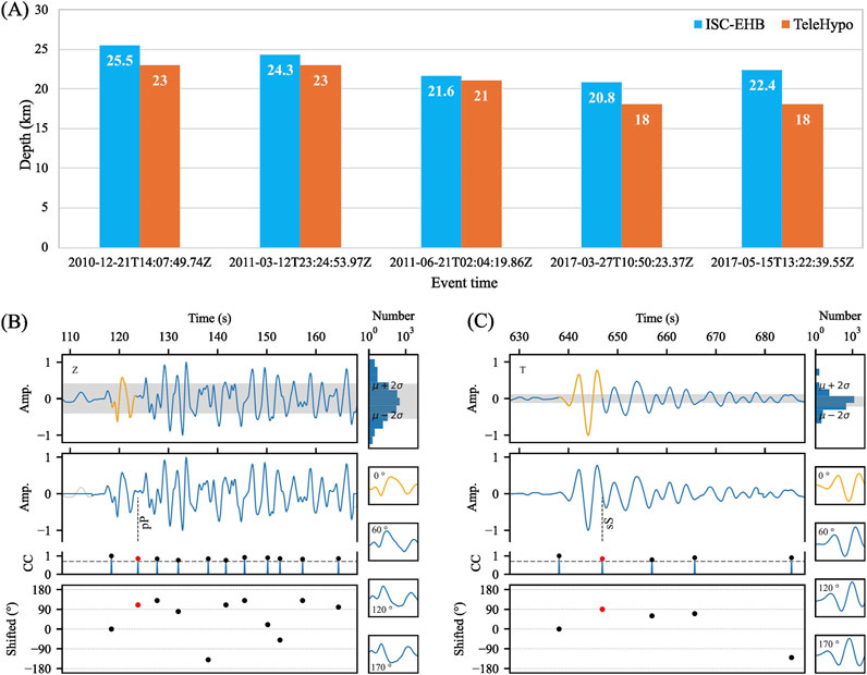
Figure 10. The depth solutions for 5 shallow earthquakes located by ISC-EHB (The blue histograms in (A)) and TeleHypo (The orange histograms in (A)). TeleHypo obtained pP (B) and sS (C) depth phases by matching the data from station N4.P46A of the fourth earthquake event (2017-03-27T10:50:23.37Z) in (A).

To investigate the depth phase identification of TeleHypo for shallow events, we analyzed the depth phase matching process of the event of 2017-03-27T10:50:23.37Z in Figure 10. The Z-component record of station N4.P46A of the event (Figure 10B) shows obvious direct P-waves (The orange waveform in Figure 10B). We obtained the pP phase through template matching (The red dot and dashed line in Figure 10B). As the source depth of this event was only 18 km, the pP phase followed closely behind the direct P-wave. The direct S-wave (The orange waveform in Figure 10C) and sS phase (The red dot and dashed line in Figure 10C) in the T-component record also exhibit similar characteristics. This means that shallow earthquakes with a focal depth of 18 km are approaching the depth location limit of TeleHypo. If the source is too shallow, there may be interference between the direct waves and depth phases, leading to waveform distortion and potentially causing TeleHypo to fail. In addition, when the direct wave or depth phase is not obvious, TeleHypo may also fail due to the inability to match the correct phase.

5 Conclusion

In this paper, we propose a new approach, TeleHypo, for automatic teleseismic precise location by integrating the advantages of two near-regional earthquake location methods, i.e., S-SNAP and DSA. During the location process, TeleHypo firstly selects high S/N and reasonably distributed stations. Then it performs preliminary scanning for the earthquake hypocenter using the data from these selected stations, and finally achieves precise hypocenter location by automatically matching depth phases. We tested the correctness of TeleHypo using an earthquake example occurred in Chile, and then further validated the applicability and practicality of this method through 54 global teleseismic events. The location capability of TeleHypo under different numbers of stations and velocity models are analyzed. The results show that TeleHypo has a good robust performance. Besides, the high-quality phase samples picked by TeleHypo can serve research on the identification of depth phases for artificial intelligence, and focal mechanism- or velocity-inversion for different seismogenic regions worldwide.

Data availability statement

The raw data supporting the conclusions of this article will be made available by the authors, without undue reservation.

Author contributions

JLY: Funding acquisition, Writing – original draft, Writing – review and editing. HM: Writing – review and editing, Software, Validation. JSY: Funding acquisition, Writing – review and editing. ZL: Data curation, Writing – review and editing. SZ: Data curation, Writing – review and editing.

Funding

The author(s) declare that financial support was received for the research and/or publication of this article. This research is supported by the Sichuan Science and Technology Program, China (2025ZNSFSC0314 to J Yuan and 2025HJPJ0007 to J Yu).

Acknowledgments

We thank Chenqi Tian for helping downloading and testing teleseismic data. Waveform data used in this study were downloaded from the Data Management Center of the Incorporated Research Institutions for Seismology(last accessed 1 November 2024). The Obspy and Matplotlib software packages are used in data processing and generating figures, respectively (Beyreuther et al., 2010; Hunter, 2007).

Conflict of interest

The authors declare that the research was conducted in the absence of any commercial or financial relationships that could be construed as a potential conflict of interest.

Generative AI statement

The author(s) declare that no Generative AI was used in the creation of this manuscript.

Publisher’s note

All claims expressed in this article are solely those of the authors and do not necessarily represent those of their affiliated organizations, or those of the publisher, the editors and the reviewers. Any product that may be evaluated in this article, or claim that may be made by its manufacturer, is not guaranteed or endorsed by the publisher.

Supplementary material

The Supplementary Material for this article can be found online at: https://www.frontiersin.org/articles/10.3389/feart.2025.1539581/full#supplementary-material

References

Baillard, C., Crawford, W. C., Ballu, V., Hibert, C., and Mangeney, A. (2014). An automatic kurtosis-based p-and s-phase picker designed for local seismic networks. Bull. Seismol. Soc. Am. 104, 394–409. doi:10.1785/0120120347

CrossRef Full Text | Google Scholar

Beyreuther, M., Barsch, R., Krischer, L., Megies, T., Behr, Y., and Wassermann, J. (2010). Obspy: a python toolbox for seismology. Seismol. Res. Lett. 81, 530–533. doi:10.1785/gssrl.81.3.530

CrossRef Full Text | Google Scholar

Craig, T. (2019). Accurate depth determination for moderate-magnitude earthquakes using global teleseismic data. J. Geophys. Res. Solid Earth 124, 1759–1780. doi:10.1029/2018jb016902

CrossRef Full Text | Google Scholar

Dziewonski, A. M., and Anderson, D. L. (1981). Preliminary reference earth model. Phys. earth Planet. interiors 25, 297–356. doi:10.1016/0031-9201(81)90046-7

CrossRef Full Text | Google Scholar

Engdahl, E. R., Di Giacomo, D., Sakarya, B., Gkarlaouni, C. G., Harris, J., and Storchak, D. A. (2020). Isc-ehb 1964–2016, an improved data set for studies of earth structure and global seismicity. Earth Space Sci. 7, e2019EA000897. doi:10.1029/2019ea000897

CrossRef Full Text | Google Scholar

Florez, M. A., and Prieto, G. A. (2017). Precise relative earthquake depth determination using array processing techniques. J. Geophys. Res. Solid Earth 122, 4559–4571. doi:10.1002/2017jb014132

CrossRef Full Text | Google Scholar

Font, Y., Kao, H., Lallemand, S., Liu, C.-S., and Chiao, L.-Y. (2004). Hypocentre determination offshore of eastern taiwan using the maximum intersection method. Geophys. J. Int. 158, 655–675. doi:10.1111/j.1365-246x.2004.02317.x

CrossRef Full Text | Google Scholar

He, X., and Ni, S. (2017). Rapid rupture directivity determination of moderate dip-slip earthquakes with teleseismic body waves assuming reduced finite source approximation. J. Geophys. Res. Solid Earth 122, 5344–5368. doi:10.1002/2016jb013924

CrossRef Full Text | Google Scholar

He, X., Zhang, P., Ni, S., and Zheng, W. (2019). Resolving focal depth in sparse network with local depth phase spl: a case study for the 2011 mineral, Virginia, earthquake sequence. Bull. Seismol. Soc. Am. 109, 745–755. doi:10.1785/0120180221

CrossRef Full Text | Google Scholar

Heyburn, R., and Bowers, D. (2008). Earthquake depth estimation using the f trace and associated probability. Bull. Seismol. Soc. Am. 98, 18–35. doi:10.1785/0120070008

CrossRef Full Text | Google Scholar

Hunter, J. D. (2007). Matplotlib: a 2d graphics environment. Comput. Sci. and Eng. 9, 90–95. doi:10.1109/mcse.2007.55

CrossRef Full Text | Google Scholar

Kao, H., and Chen, W.-P. (1991). Earthquakes along the ryukyu-kyushu arc: strain segmentation, lateral compression, and the thermomechanical state of the plate interface. J. Geophys. Res. Solid Earth 96, 21443–21485. doi:10.1029/91jb02164

CrossRef Full Text | Google Scholar

Kao, H., and Shan, S.-J. (2004). The source-scanning algorithm: mapping the distribution of seismic sources in time and space. Geophys. J. Int. 157, 589–594. doi:10.1111/j.1365-246x.2004.02276.x

CrossRef Full Text | Google Scholar

Kennett, B., and Engdahl, E. (1991). Traveltimes for global earthquake location and phase identification. Geophys. J. Int. 105, 429–465. doi:10.1111/j.1365-246x.1991.tb06724.x

CrossRef Full Text | Google Scholar

Kennett, B. L., Engdahl, E., and Buland, R. (1995). Constraints on seismic velocities in the earth from traveltimes. Geophys. J. Int. 122, 108–124. doi:10.1111/j.1365-246x.1995.tb03540.x

CrossRef Full Text | Google Scholar

Krischer, L., Megies, T., Barsch, R., Beyreuther, M., Lecocq, T., Caudron, C., et al. (2015). Obspy: a bridge for seismology into the scientific python ecosystem. Comput. Sci. and Discov. 8, 014003. doi:10.1088/1749-4699/8/1/014003

CrossRef Full Text | Google Scholar

Letort, J., Guilbert, J., Cotton, F., Bondár, I., Cano, Y., and Vergoz, J. (2015). A new, improved and fully automatic method for teleseismic depth estimation of moderate earthquakes (4.5 < m < 5.5): application to the guerrero subduction zone (Mexico). Geophys. J. Int. 201, 1834–1848. doi:10.1093/gji/ggv093

CrossRef Full Text | Google Scholar

Shelly, D. R., Beroza, G. C., and Ide, S. (2007). Non-volcanic tremor and low-frequency earthquake swarms. Nature 446, 305–307. doi:10.1038/nature05666

PubMed Abstract | CrossRef Full Text | Google Scholar

Smith, G. P., and Ekström, G. (1997). Interpretation of earthquake epicenter and cmt centroid locations, in terms of rupture length and direction. Phys. earth Planet. interiors 102, 123–132. doi:10.1016/s0031-9201(96)03246-3

CrossRef Full Text | Google Scholar

Tan, F., Kao, H., Nissen, E., and Eaton, D. (2019). Seismicity-scanning based on navigated automatic phase-picking. J. Geophys. Res. Solid Earth 124, 3802–3818. doi:10.1029/2018jb017050

CrossRef Full Text | Google Scholar

Yuan, J., Kao, H., and Yu, J. (2020). Depth-scanning algorithm: accurate, automatic, and efficient determination of focal depths for local and regional earthquakes. J. Geophys. Res. Solid Earth 125, e2020JB019430. doi:10.1029/2020jb019430

CrossRef Full Text | Google Scholar