InSAR-constrained parallel elastic finite element models for fault coseismic dislocation inversion: a case study of the 2016 MW 5.9 Menyuan earthquake

The study of fault coseismic dislocation distribution is crucial for understanding fault stress release, fault sliding behavior, and surface deformation during seismic events. This knowledge is essential for engineering design and disaster prevention. Traditional seismic dislocation theories, which assume a uniform elastic semi-infinite space, fail to account for topographic relief, medium inhomogeneity in the seismic source area. In contrast, parallel elastic finite element models effectively address these complexities by accommodating geometric, material, and boundary condition variations, offering high spatial resolution and efficient computation. In this paper, we introduce a novel fault coseismic dislocation inversion method based on parallel elastic finite element simulations. We conduct inversion tests using several idealized fault models to validate our approach. Applying this method to the 2016 M_W 5.9 Menyuan earthquake, we successfully invert the coseismic dislocation distributions. Our results align with previous studies and show excellent agreement with InSAR coseismic observations, thereby confirming the method’s validity. Ideal model tests demonstrate that a 10% Young’s modulus contrast across fault interfaces significantly affects coseismic dislocation inversion. Topographic relief exhibits limited influence on the coseismic dislocation inversion of the 2016 Menyuan M_W 5.9 earthquake. The distinct mechanical responses of material heterogeneity and topographic effects require separate quantification, confirming our method’s viability for coseismic dislocation inversion in actual large earthquakes.

1 Introduction

The inversion of coseismic dislocation in seismic faults is a key area of interest in earthquake science, playing a critical role in understanding the rupture process, surface deformation during earthquakes, and the characterization of seismic source parameters. This knowledge is essential for effective earthquake prevention and disaster mitigation. Accurately capturing the inhomogeneity and geometric complexity of the Earth’s medium is crucial for realistic modeling of seismogenic faults. Therefore, there is a need to develop a numerical simulation-based method for coseismic dislocation inversion that reflects these complexities.

Medium inhomogeneity and geometrical complexity exert distinct influences on both numerical Green’s function computation and coseismic fault dislocation inversion processes. Some studies employing finite-element codes to generate Green’s functions have demonstrated that topography has a relatively small effect, reducing seismic potency by approximately 5% compared with a flat model for a shallow slow slip events offshore of the North Island of New Zealand (Williams and Wallace, 2018). But the impact of topography could be highly significant for steep slopes, particularly in regions with significant topographic relief (>500 m) (Moreno et al., 2012; Ragon and Simons, 2021). The incorporation of material heterogeneity derived from a New Zealand-wide seismic velocity model reveals substantial amplification effects, with seismic potency enhancements exceeding 58% (Williams and Wallace, 2018). The effects of 3D crustal heterogeneity (Masterlark, 2003; Ragon and Simons, 2021), basin media heterogeneity, and structural tectonics (Langer et al., 2023) on coseismic dislocation inversion are very different and unique, which indicates that independent and individualized case studies are required and cannot be generalized. Additionally, investigations employing 3D spherical finite element models to invert the coseismic slip distribution of the 2010 M_W 8.8 Maule earthquake along the Nazca-South America plate boundary revealed non-negligible Earth curvature effects when rupture lengths approach 500 km (Moreno et al., 2012). A representative study is the coseismic dislocation inversion of the 2015 Gorkha, Nepal earthquake, which simultaneously accounted for the influences of topography and material heterogeneity (Wang and Fialko, 2018; Langer et al., 2019). Some scholars employed the Gamra finite-difference framework (Landry and Barbot, 2016) to construct elastostatic Green’s functions linking subsurface deformation to surface displacements, utilizing adaptive meshing and Immersed Interface Method adaptations (Leveque and Li, 1994) to resolve fault-slip singularities, constraining the Sierra Madre-Puente Hills-Compton thrust system’s long-term slip rate (3–4 mm/yr) and current partial locking in upper sections consistent with interseismic strain accumulation (Rollins et al., 2018).

A high-resolution 3D finite element model (FEM) constrained by coseismic GNSS, Sentinel-1 DInSAR, and pixel offset data is implemented for sequential fault slip inversion of the 2019 Ridgecrest earthquake sequence complex fault surface ruptures. The optimal solution is derived through heterogeneous FEM modeling and fused geodetic datasets combining pixel offsets, interferograms, and GNSS measurements (Barba-Sevilla et al., 2022). Some scholars employed idealized (M1A-M1D) and regional (GEONET, M2A-M2H) kinematic finite-source models to quantify grid-size effects on slip distributions and resolves the 2011 M_W 9.0 Tohoku-oki slip distribution through Bayesian-optimized finite-element modeling integrating terrestrial and seafloor geodetic data, demonstrating enhanced capacity to reconcile near-trench slip deficits while addressing grid-dependent resolution limits in coseismic inversions (Kim et al., 2024). The 2008 M_W 7.9 Wenchuan earthquake source is inverted through integration of strong-motion waveforms, geodetic offsets, and 3D synthetic ground motions. A multi-time-window approach is implemented with static/dynamic Green’s functions derived from finite-element modeling, incorporating reciprocity principles and strain tensor formulations. The rupture process is systematically constrained by combined utilization of complex fault geometry, GPS/strong-motion datasets, and 3D heterogeneous structure (Ramirez-Guzman and Hartzell, 2020).

Coseismic dislocation inversion is a powerful technique for accurately mapping fault dislocation distributions during earthquakes, thus elucidating fault rupture mechanisms and sliding processes. For instance, the inversion of slip distribution for the 2011 M_W 9.0 Tohoku earthquake, using GPS and InSAR data, highlighted the extensive rupture area and provided crucial insights into tsunami generation (Ozawa et al., 2011). Similarly, GPS and InSAR data have been used to invert the coseismic fault dislocations and associated surface deformation for the 2008 M_W 7.9 Wenchuan earthquake and the 2015 M_W 7.8 Gorkha earthquake (Wan et al., 2017; Duan et al., 2020; Hong and Liu, 2021; Shi et al., 2023). These studies are of significant theoretical importance for understanding earthquake rupture propagation and source mechanisms, including strike-slip, thrust, and normal faulting.

Coseismic dislocation inversion is instrumental in studying the triggering effects of earthquakes. Large earthquakes can trigger seismic events on adjacent faults through the mechanism of coseismic stress transfer. By analyzing coseismic slip and its impact on nearby faults, we can gain deeper insights into the mechanisms behind earthquake swarms and the formation of earthquake sequences (King et al., 1994; Stein, 1999; Freed, 2005).

Currently, the inversion of coseismic dislocations for seismogenic faults predominantly relies on the Okada analytical model of elastic uniform semi-infinite space (Okada, 1992; Niu et al., 2016; Li and Barnhart, 2020). This model is favored for its simplicity and the high accuracy and efficiency of its Green’s function calculations. However, a limitation of this approach is its inability to account for medium heterogeneity, particularly lateral inhomogeneities on either side of the fault, and the complex geometry of surface undulations. These constraints systematically bias both forward models and inverse solutions, particularly in regions with significant topographic relief (>500 m) or strong material heterogeneity (Masterlark, 2003; Moreno et al., 2012; Williams and Wallace, 2018; Ragon and Simons, 2021).

The Green’s function for coseismic dislocation inversion of seismic faults can be determined using the analytical solution from Okada’s seismic dislocation theory or through numerical methods like finite elements. Observation data typically include coseismic GPS, InSAR, or a combination of both. Based on these inputs, the inversion process commonly employs the least squares method with smooth constraints (Niu et al., 2016; Zuo et al., 2016; Duan et al., 2020).

Some researchers have developed a coseismic dislocation inversion method for originating faults utilizing both far-field seismic and near-field strong-motion waveform data (Zhang et al., 2012; Zhang et al., 2014; Tilmann et al., 2016). Fault dislocation inversion methods comprise several approaches, including the steepest descent method, synoptic dislocation inversion using triangular mesh faults, techniques for updating mesh configurations, and methods employing Bayesian probabilistic models to invert fault geometric parameters.

The Earth’s medium exhibits significant inhomogeneities, particularly lateral ones, with considerable differences in material parameters on either side of an earthquake-generating fault. For instance, the 2008 Wenchuan earthquake along the Longmenshan Fault demonstrated significant lateral variations, with topographic relief differences exceeding 4,000 m (Shi et al., 2023). Okada’s ideal model does not account for such lateral inhomogeneities and topographic variations, as well as the undulations of major structural surfaces within the Earth’s interior. Consequently, the use of numerical simulations for coseismic dislocation inversion of seismogenic faults has become a prominent research focus in earthquake science. This paper introduces a novel method for coseismic dislocation inversion based on finite element numerical simulation. We validate the accuracy of this new inversion method using an ideal model and apply it to analyze the fault coseismic dislocation distribution of the 2016 Menyuan M_W 5.9 earthquake (Figure 1).

Figure 1

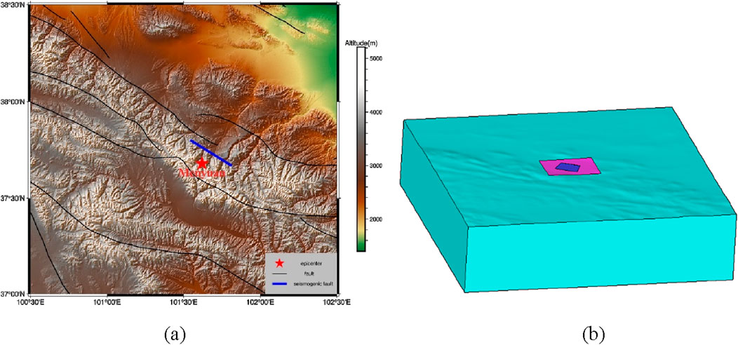
Figure 1. Tectonic setting and 3D topography-incorporated finite element model of the 2016 M_W 5.9 Menyuan earthquake. (a) Tectonic setting (modified from Luo and Wang, 2022); (b) 3D topography-incorporated finite element model.

2 Methods for fault coseismic dislocation inversion using parallel elastic finite element simulation

2.1 Fundamental equations for fault coseismic dislocation inversion

In this paper, we employ a fault coseismic dislocation inversion method using parallel elastic finite element simulation. The fault is divided into k sub-faults, with the inversion parameters represented as m. For the ith sub-fault (i = 1, k), the dislocation components along the strike and dip are denoted as $m_{is}$ and $m_{id}$, respectively. Here, the subscript i refers to the ith sub-fault, while s and d indicate the strike and dip components. The ground surface coseismic displacements are measured at n observation points, represented as d. At the jth observation point, the observed surface displacement components are $d_{jx}$, $d_{jy}$ and $d_{jz}$, where j stands for the jth observation point (j = 1, n), and x, y, z represent the eastward, northward, and upward directions, respectively. The Green’s function for inversion is denoted as G. For a unit dislocation of the ith sub-fault at the jth observation point, the Green’s function components are $g_{jx.is}$, $g_{jy.is}$, $g_{jz.is}$, $g_{jx.id}$, $g_{jy.id}$ and $g_{jz.id}$. The indices i, j, x, y, z, d, and s have the same definitions as before.

In coseismic fault dislocation inversion, the relationship between the coseismic surface displacement data d and slip parameters m is mathematically formulated as (Tikhonov, 1963; Tilmann et al., 2016; Li and Barnhart, 2020):

$\mathbf{d}=\mathbf{Gm}+\mathbf{\epsilon }(1)$

where d denotes InSAR-derived Line-of-Sight (LOS) deformation measurements or three-component GPS displacement vectors, G represents the Green’s function coefficient matrix, m corresponds to the slip parameters of sub-faults (Strike-slip component, Dip-slip component), and ε encapsulates observational uncertainties. The specific expressions for d, m, G are given in Equations 2–4.

${\mathit{d}}_{\left(3n*1\right)}=\left[\begin{array}{c}{d}_{1x}\\ d_{1y}\\ d_{1z}\\ \dots \\ d_{nx}\\ d_{ny}\\ d_{nz}\end{array}\right](2)$

${\mathit{m}}_{\left(2k*1\right)}=\left[\begin{array}{c}{m}_{1s}\\ m_{1d}\\ \dots \\ m_{ks}\\ m_{kd}\end{array}\right](3)$

where s and d represent the strike and dip components of dislocation, respectively, and x, y, z indicate the components of surface displacement in the eastward, northward, and upward directions.

The Green’s function matrix G is:

$\mathit{G}\left(3n*2k\right)=\left[\begin{array}{cccccc}{g}_{1x.1s}& \dots & g_{1x.ks}& g_{1x.1d}& \dots & g_{1x.kd}\\ g_{1y.1s}& \dots & g_{1y.ks}& g_{1y.1d}& \dots & g_{1y.kd}\\ g_{1z.1s}& \dots & g_{1z.ks}& g_{1z.1d}& \dots & g_{1z.kd}\\ \dots & \dots & \dots & \dots & \dots & \dots \\ g_{nx.1s}& \dots & g_{nx.ks}& g_{nx.1d}& \dots & g_{nx.kd}\\ g_{ny.1s}& \dots & g_{ny.ks}& g_{ny.1d}& \dots & g_{ny.kd}\\ g_{nz.1s}& \dots & g_{nz.ks}& g_{nz.1d}& \dots & g_{nz.kd}\end{array}\right](4)$

where subscripts x, y, z, d, and s are the same as above.

In practical inversion applications, it is generally required that the degrees of freedom of observation, 3n, exceed those of the inversion parameters, 2 k. This condition is met when the number of observations exceeds the number of inversion parameters, allowing m to be calculated using the least squares method:

$\mathit{m}={\left({\mathit{G}}^{\mathrm{T}}\mathit{G}\right)}^{-1}{\mathit{G}}^{\mathrm{T}}\mathit{d}(5)$

2.2 Calculation of the green’s function G

We developed a parallel elastic finite element program to compute coseismic displacements and stresses, considering factors such as topographic relief, medium inhomogeneity, and non-uniform dislocation distributionusingthe split-node technique (Melosh and Raefsky, 1981; Shi et al., 2023). This program allows us to calculate the numerical displacement Green’s function for any subfault dislocation at surface observation points, using parameters like fault dislocation, length, width, dip, strike angle, and slip angle. A key feature of this paper is the use of a 3D parallel finite element model to calculate these functions, fully accounting for the effects of topographic relief, medium inhomogeneity, complex fault geometry, and dislocation distribution. This approach enhances the realism of fault dislocation inversion results.

2.3 Regularization method for fault coseismic dislocation inversion

The fault coseismic dislocation distributions obtained by direct inversion using the least squares method Equation 5 are often pathologized by Equation 1 because of the overly strong linear correlation of some rows of the Green’s function G matrix. In order to reduce the effect of this pathology, a Tikhonov regularization term is often added to the inversion (Tikhonov, 1963):

$\left[\begin{array}{c}\mathit{G}\\ \alpha \mathit{L}\end{array}\right]\mathit{m}=\left[\begin{array}{c}\mathit{d}\\ \mathbf{0}\end{array}\right](6)$

where α represents the regularization parameter, and L is the regularization matrix, which can be selected based on specific requirements. When L is the simplest form, a diagonal matrix I, the least squares solution for m is calculated as follows:

$\mathit{m}={\left({\mathit{G}}^{\mathrm{T}}\mathit{G}+{\alpha }^2\mathrm{I}\right)}^{-1}{\mathit{G}}^{\mathrm{T}}\mathit{d}(7)$

If the Laplace operator L = ∇² is used, the least squares solution for m is calculated as follows:

$\mathit{m}={\left({\mathit{G}}^{\mathrm{T}}\mathit{G}+{\alpha }^2{\mathit{L}}^{\mathrm{T}}\mathit{L}\right)}^{-1}{\mathit{G}}^{\mathrm{T}}\mathit{d}(8)$

2.4 Determination of regularization parameters

For general linear least-squares problems, there may be infinitely many least-squares solutions. Considering that data contain noise and precisely fitting such noise is meaningless, the Tikhonov regularization linear inversion method is a mathematical technique that stabilizes the inversion process by introducing smoothness constraints. The core principle of this method lies in pursuing the match between model parameters and observed data while enforcing gradual variation of parameter values between adjacent spatial locations, thereby preventing solutions from exhibiting severe oscillations or overfitting noise. Specifically, the system balances data fitting accuracy and model smoothness through an adjustable weighting coefficient (regularization parameter): when the weight is increased, inversion results show high continuity but may lose details; when the weight is reduced, model details become richer but may amplify data errors. This method is particularly suited for scenarios requiring continuous gradual features, such as velocity structure reconstruction in geophysical exploration and earthquake source slip distribution inversion. Its advantages include computational efficiency and solution uniqueness, while its limitation lies in reduced resolution for anomalies with sharp boundaries, potentially causing edge blurring.

How to find the regularization parameter of Equations 6–8 is the key to fault coseismic dislocation inversion. In seismic slip distribution inversion, there are numerous methods used to determine the regularization parameter. Allen (1974) first proposed to use the Generalized Cross Validation (GCV) method to find the regularization parameter (Allen, 1974), which is able to obtain a more ideal regularization parameter (Golub et al., 1979; Fan et al., 2017). In addition, the variance component estimation method was first proposed by Helmert (1907) for determining the posterior variance of the data, which is more effective for fault coseismic dislocation inversion (Xu et al., 2019; Xu et al., 2019; Xu et al., 2019; Fan et al., 2017). Determining the regularization parameter in Equations 6–8 is crucial for fault coseismic dislocation inversion. In seismic slip distribution inversion, various methods exist for this purpose. Allen (1974) first introduced the Generalized Cross Validation (GCV) method to identify an optimal regularization parameter (Golub et al., 1979; Fan et al., 2017).

In fault coseismic slip distribution inversion, the L-curve method is widely used due to its computational simplicity. Introduced by Hansen in 1992, this method effectively addresses the inversion of ill-posed equations (Hansen, 1992). It has been applied in geodetic surveying and is currently used in gravity downward continuation, image smoothing, and slip distribution inversion to determine regularization parameters (Hansen and O’leary, 1993). In this study, the L-curve method is also employed to determine the regularization parameters for fault dislocation inversion.

2.5 Inversion steps

(1) Collect surface coseismic GPS or InSAR observation data d.

(2) Divide the seismogenic fault into k subfaults, forming a column vector m with 2 k components.

(3) Use a 3D parallel elastic finite element model to compute the Green’s function G for the unit dislocation in both the strike and dip components of each subfault at the surface observation points.

(4) Determine the strike and dip dislocations m for all subfaults by plotting L-curves using Equations 6–8.

3 Coseismic dislocation inversion for the 2016 Mengyuan M_W 5.9 earthquake

3.1 The background and coseismic deformation observation of the earthquake

On 12 January 2016, an earthquake of magnitude M_W5.9 occurred under the Lenglongling Mountains in Menyuan County, China (Figure 1). Previous studies have shown that the mechanism of the 2016 M_W5.9 earthquake was purely thrust-slip (e.g., Li et al., 2016; Zhang et al., 2020). A more accurate inversion of the fault coseismic dislocation can better characterize the coseismic rupture process and source mechanism of this earthquake. The raw Sentinel-1 satellite data were obtained from the European Space Agency (ESA) and were processed using Sentinel-1 Interferometry Processor (Jiang et al., 2017; Luo and Wang, 2022). The dates of the SAR images of AT128 and DT33 are 2016/01/13-2016/02/06, 2016/01/18-2016/02/11, both of which contain the onset time of this earthquake, can be used to calculate the surface coseismicity caused by this earthquake.

Sentinel-1 SAR images were processed using the Sentinel-1 interferometry processor (http://sarimggeodesy.github.io/software) (Jiang et al., 2017). Luo and Wang (2022) obtained the main geometric information of the fault from which the earthquake originated using a Bayesian approach: an optimal model shows the push-slip mechanism on a low-angle, south-dipping fault plane (strike = 122°, dip = 43°) with a length of 28.5 km and a width of 16.5 km. The fault was inverted in a Bayesian framework using geodetic Bayesian inversion software (Bagnardi and Hooper, 2018). The InSAR observation has just recorded the coseismic surface deformation of this earthquake, which provides the most valuable observational data for inverting the distribution of fault coseismic dislocations of this earthquake. This provides the most valuable observation data for the inversion of the fault coseismic dislocation distribution of this earthquake.

3.2 Two checkerboard tests of fault coseismic dislocation inversion

To validate the proposed fault coseismic dislocation inversion method using parallel elastic finite element numerical simulation, we segmented the source fault of the 2016 Mengyuan earthquake into 20 larger subfaults, comprised of 19*16 basic subfaults. We developed two ideal fault coseismic dislocation models and utilized a three-dimensional elastic parallel finite element program to generate theoretical surface observations (Figure 2). This program was also used to calculate the numerical Green’s function for unit dislocations in subfault strike and dip, enabling us to evaluate the accuracy of our inversion method.

Figure 2

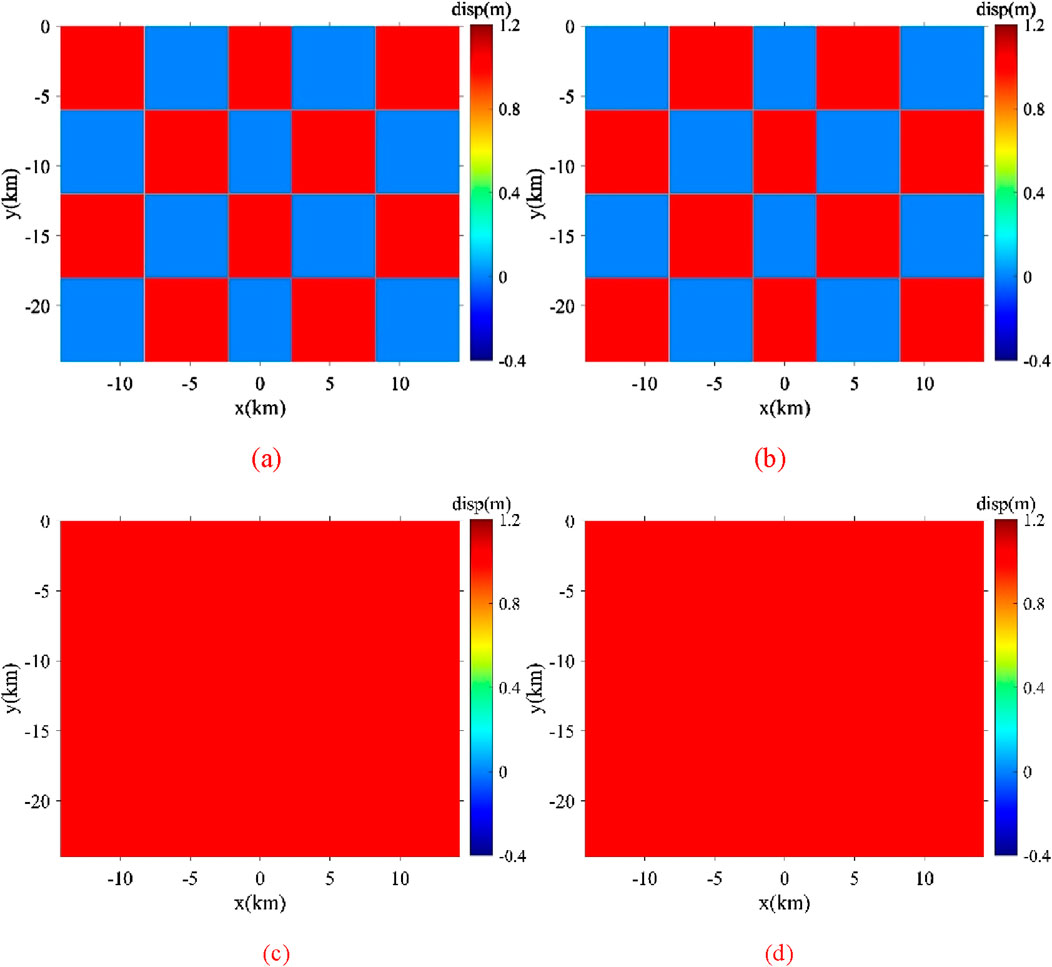
Figure 2. Ideal fault coseismic dislocation models: (a, b) show the dislocation distribution along the strike and dip for the model of intersecting distributed dislocations; (c, d) depict the distribution along the strike and dip for the homogeneous model.

We performed inversions of two sets of ideal fault coseismic dislocation distributions using two regularization methods. Figures 3A–C presents the results using a diagonal matrix as the L-matrix for intersecting distributed dislocations, while Figures 3D–F uses a two-dimensional Laplacian smooth matrix for the same. Figures 4A–F provide the inversion results for uniformly distributed dislocations using a diagonal matrix or 2D Laplace smooth matrix as the L-matrix, respectively. The inversion results align with the ideal fault coseismic dislocation distributions, validating the accuracy of our proposed inversion method based on parallel elastic finite element simulation.

Figure 3

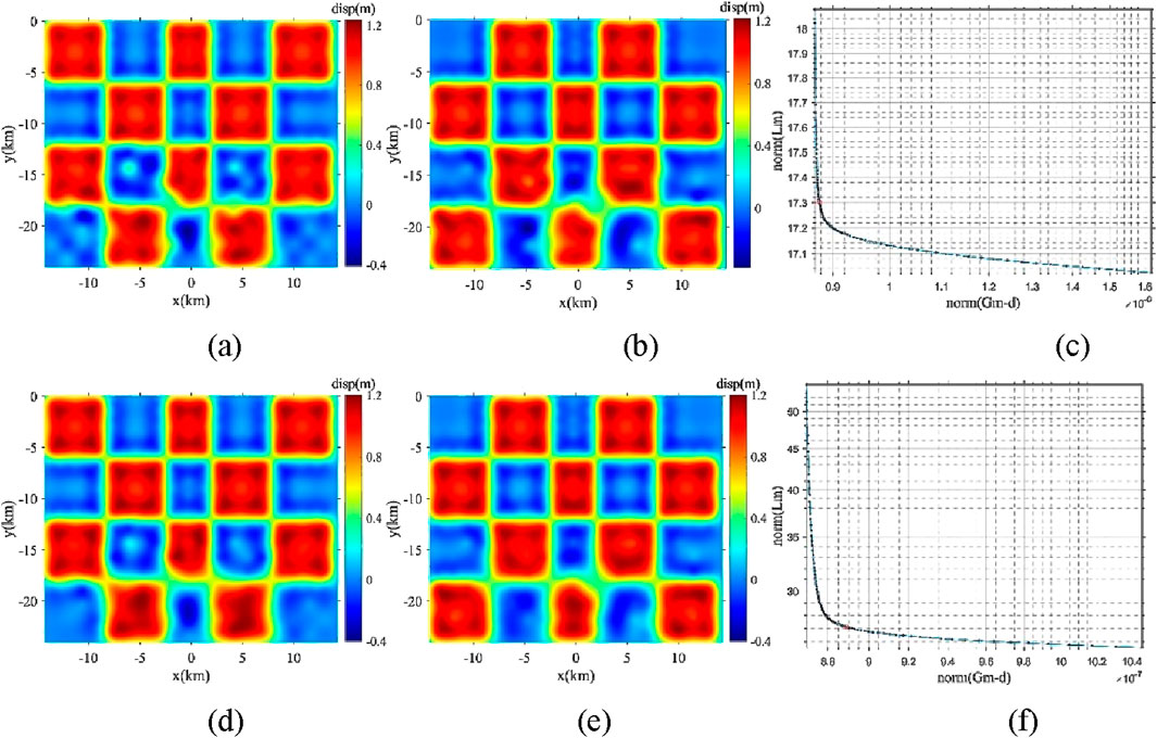
Figure 3. Inversion results for the model of intersecting distributed dislocations using a diagonal L-matrix and the 2D Laplace smooth matrix as the L-matrix. (a–c) for diagonal L-matrix: inversed coseismic dislocation along strike direction, inversed coseismic dislocation along dip direction and L-Curve, respectively. (d–f) for 2D Laplace smooth matrix as the L-matrix.

Figure 4

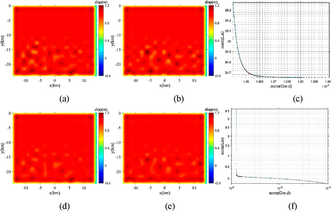
Figure 4. Inversion results for the model of uniformly distributed dislocations using a diagonal L-matrix and the 2D Laplace smooth matrix as the L-matrix. (a–c) for diagonal L-matrix: inversed coseismic dislocation along strike direction, inversed coseismic dislocation along dip direction and L-Curve, respectively. (d–f) for 2D Laplace smooth matrix as the L-matrix.

3.3 Inversion of fault coseismic dislocations for the 2016 Mengyuan M_W 5.9 earthquake using InSAR data (based on flat-topography FEM model)

Based on the two checkerboard tests of fault coseismic dislocation inversion in Section 3.2, we inverted the fault coseismic dislocations of the 2016 Mengyuan M_W 5.9 earthquake using real InSAR data. The data consists of two sets, including ascending and descending tracks (Figure 1). The fault responsible for the earthquake was divided into 19 × 8 subfaults, and the Green’s functions for surface coseismic displacements caused by unit dislocations along the strike and dip of each subfault were calculated using a three-dimensional parallel finite element program (Shi et al., 2023). For the parallel elastic finite element model of the 2016 M_W 5.9 earthquake in Mianyang with flat terrain, tetrahedral elements were used, with 1,084,231 nodes, 6,400,464 tetrahedrons, and 60 partitions. We adopted the homogeneous elastic medium with Young’s modulus E = 81 GPa, Poisson’s ratio ν = 0.25 from previous work (Luo and Wang, 2022). The total computation time for numerical Green’s function solutions was 1.54 × 10⁵ s. The parallel computing architecture of the PFELAC 2.2 platform is illustrated by Chen et al. (2025). This architecture ensures efficient parallelization while maintaining computational coherence across distributed processes. Based on the principles of domain decomposition, it adopts a modular programming approach, dividing the main program into a master process and slave processes. Each part consists of functionally distinct components. During computation, when the slave processes invoke solver programs, the master process correspondingly activates solver interface programs to ensure synchronization across the entire system (Element Computing Technology Co., Ltd, 2018).

We directly employed preprocessed InSAR data from ascending and descending tracks (AT128, DT33), downsampled to 1,951 observation points, as LOS displacement components for coseismic fault dislocation inversion (Luo and Wang, 2022). The InSAR data processing methodology follows Luo and Wang (2022). Optimized InSAR Processing & Fault Slip Inversion Workflow (Luo and Wang, 2022): 1. SAR Data Acquisition: Processed Sentinel-1 ascending (AT128) and descending (DT33) track data covering the 2016 M_W 5.9 Menyuan earthquake using Sentinel-1 Interferometry Processor (Jiang et al., 2017). 2. Coseismic Interferogram Generation: Generated differential interferograms with phase unwrapping via Statistical-cost, Network-flow Algorithm (Chen and Zebker, 2000). 3. Derived near-field surface displacements through pixel-offset tracking (Wang et al., 2014; Wang and Jonsson, 2015). 4. Data Downsampling: Applied quadtree-based downsampling to optimize computational efficiency while preserving deformation signals (Jonsson et al., 2002). 5. Fault Geometry Optimization: Performed Bayesian inversion of uniform-slip rectangular fault models (Free parameters: Strike, dip, length, width, depth, slip magnitude) in homogeneous elastic half-space using Geodetic Bayesian Inversion Software (Bagnardi and Hooper, 2018). 6. Distributed Slip Inversion: Solved slip distribution on optimized fault planes through least-squares inversion with steepest descent regularization (Wang et al., 2011).

Three inversion methods were appliedbased on Flat-topography FEM model: the diagonal matrix as the L-matrix (Figures 5A–C), the Laplace smoothing matrix as the L-matrix (Figures 5D–F), and the steepest descent method (Figures 5G, H). All three methods produced similar coseismic dislocation distributions, which are consistent with previous results (Luo and Wang, 2022), confirming the accuracy and reliability of our inversion methods.

Figure 5

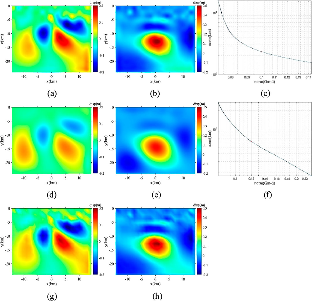
Figure 5. Fault dislocation inversion of the 2016 Mengyuan M_W 5.9 earthquakebased on flat-topography FEM model. (a–c) for diagonal L-matrix with regularization parameter 0.0331: inversed coseismic dislocation along strike direction, inversed coseismic dislocation along dip direction and L-Curve, respectively. (d–f) for 2D Laplace smooth matrix as the L-matrix with regularization parameter 0.1259. (g–h) by steepest descent method with 300 iterations.

3.4 Inversion of fault coseismic dislocations for the 2016 Mengyuan M_W 5.9 earthquake using InSAR data (based on undulating-topography FEM model)

For the 2016 M_W 5.9 Menyuan earthquake, we have additionally developed a parallel elastic finite element model incorporating actual topographic relief, computed numerical Green’s functions considering topographic relief, and inverted the coseismic fault dislocation distribution (Figure 6). We adopted the homogeneous elastic medium with Young’s modulus E = 81 GPa, Poisson’s ratio ν = 0.25 from previous work (Luo and Wang, 2022). We compared the fault dislocation inversion results between actual and flat topography, as well as the differences in the three-component surface coseismic displacement distributions. The effect of topographic relief on the inversion of fault coseismic dislocations is small and almost negligible for the 2016 Mengyuan earthquake.

Figure 6

Figure 6. Fault dislocation inversion of the 2016 Mengyuan M_W 5.9 earthquake based on undulating-topography FEM model. (a–c) for diagonal L-matrix with regularization parameter 0.0331: inversed coseismic dislocation along strike direction, inversed coseismic dislocation along dip direction and L-Curve, respectively. (d–f) for 2D Laplace smooth matrix as the L-matrix with regularization parameter 0.1259. (g–h) by steepest descent method with 300 iterations.

4 Discussion

4.1 Advantages and disadvantages of different inversion methods

In the study of coseismic dislocation distribution, several inversion methods are available, each with distinct features. The Least Squares Method (LSM) is foundational, offering computational simplicity and efficiency but is sensitive to noise, risking overfitting (Minato et al., 2020). The Damped Least Squares Method (DLSM) enhances result stability through a damping parameter, though its selection is experience-based (Deo and Walker, 1995). The Smoothed Constrained Least Squares (SLSM) method suppresses high-frequency noise with smoothing constraints, ideal for smoother dislocation scenarios, yet may overly smooth and obscure local details (Harris and Segall, 1987).

The Steepest Descent Method (SDM), used in nonlinear inversion, is straightforward and suitable for initial solutions, but is slow in convergence and prone to local optima (Quiroz et al., 2008). The triangular mesh refinement method increases resolution for complex fault geometries, though at a high computational cost (Zuo et al., 2016). Bayesian Inversion (BI) effectively manages uncertainty by integrating prior information with observations, yet its complexity and reliance on model assumptions are significant (Duan et al., 2020).

In summary, the choice of inversion method should be scenario-specific, balancing various factors. This study applies Damped Least Squares (DLSM), Smoothed Least Squares (SLSM), and the Steepest Descent Method (SDM) to the fault coseismic dislocation distribution of the 2016 M_W 5.9 earthquake. The simulated displacements align well with InSAR observations, demonstrating the adaptability of the proposed finite element-based inversion approach.

4.2 Rationale for selecting the finite element model-based inversion method

We employ a parallel elastic finite element model, a numerical framework that extends beyond simple analytical solutions. This approach fully utilizes the unique advantages of finite element methodology, enabling effective integration of real surface undulation and elastic medium inhomogeneity into coseismic deformation modeling for large earthquakes. Through parallel computing technology, we implement large-scale numerical simulations with millions of grid nodes while maintaining mesh resolution and computational accuracy, resulting in strong consistency between simulation outputs and geodetic observations such as InSAR data.

To evaluate the impact of lateral inhomogeneity on fault coseismic dislocation inversion, we compared numerical Green’s function solutions using a uniform elasticity model (Model 1) and a lateral inhomogeneous elasticity model (Model 2) (Figure 7). 1) Homogeneous Model (Model 1):Homogeneous elastic medium with Young’s modulus E = 81 GPa, Poisson’s ratio ν = 0.25 (representative of upper crustal rocks); 2) Heterogeneity Model (Model 2): Laterally stratified structure across fault strike, Hanging wall: E = 85.05 GPa (+5% perturbation), Footwall wall: E = 76.95 GPa (−5% perturbation), Far-field host rock: E = 81 GPa (maintaining continuum consistency), Identical ν = 0.25 throughout.

Figure 7

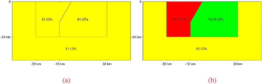
Figure 7. Benchmark tests of medium heterogeneity effects on coseismic slip inversion across fault zones (a) Homogeneous model (Model1); (b) Heterogeneous model (Model 2). The numerical values in GPa represent the Young’s modulus of respective regions. All domains maintain a uniform poisson’s ratio of 0.25.

We applied these models to invert fault coseismic dislocation across a consistent grid of 6 × 6 = 36 subfaults. The seismic displacement data at 100 surface observation points were synthetically generated using Model 2. With these observations fixed, we computed the numerical Green’s functions for both Model 1 and Model 2. Figure 8 illustrates the resulting fault coseismic dislocation distributions. The uniform elasticity model (Model 1) shows significant bias, leading to incorrect inversion results. In contrast, the lateral inhomogeneous elasticity model (Model 2) yields highly accurate dislocation distributions, closely matching the predefined fault intersection dislocations. These dual experimental configurations of coseismic fault dislocation inversion utilizing the identical observational dataset demonstrate with clarity that medium heterogeneity exerts substantial influence on the inversion outcomes. To obtain the identical observational dataset, we used an intersecting distributed dislocations with 0 m and 1 m along both the along the strike and dip. This comparison highlights the significant influence of medium inhomogeneity on dislocation inversion, underscoring the effectiveness of using a finite element model-based approach in such analyses.

Figure 8

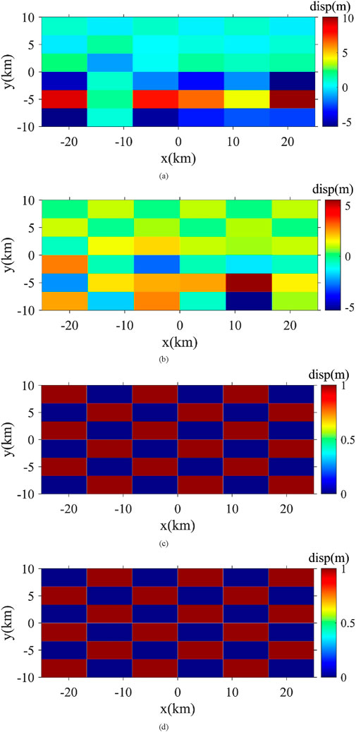
Figure 8. Comparison of fault dislocation inversion based on uniformity model 1 and non-uniformity model 2. (a) Inversed coseismic dislocation along strike direction by Model 1; (b) inversed coseismic dislocation along dip direction by Model 1; (c) inversed coseismic dislocation along strike direction by Model 2; (d) inversed coseismic dislocation along dip direction by Model 2.

4.3 The comparison of flat-topography FEM and undulating-topography FEM with InSARobservation

Notably, our comparative analyses of fault displacement components along satellite line-of-sight directions reveal critical insights when evaluating ascending/descending InSAR data from the 2016 M_W 5.9 Menyuan event against finite-element simulations. The displacement patterns and residual distributions (Figure 9: flat-topography FEM model; Figure 10: topography-incorporated FEM model) demonstrate remarkable consistency with the kinematic models proposed by Luo and Wang (2022), particularly in terms of near-field deformation characteristics. This agreement persists despite our implementation of a topography-incorporated finite element approach - a critical refinement that enhances dislocation inversion precision through explicit consideration of surface elevation gradients. The root mean square error (RMSE) between finite element simulations and InSAR-derived LOS displacements at 1,951 surface observation points is 2.71071210902590 × 10⁻³ m and 2.70929434322033 × 10⁻³ m for flat-topography and topography-incorporated FEM models, respectively. Our analysis demonstrates that topographic variations exert limited influence on coseismic fault dislocation inversion results (≤5% discrepancy), aligning with established methodological frameworks (Williams and Wallace, 2018).

Figure 9

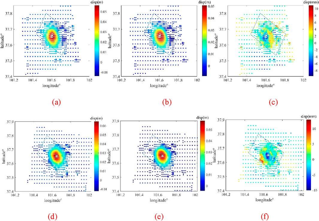
Figure 9. InSAR vs flat-topography FEM LOS displacements with residuals: 2016 M_W 5.9 Menyuan earthquake. Surface-projected fault traces are delineated by blue polygons. The root mean square error (RMSE) between finite element simulations and InSAR-derived LOS displacements at 1,951 surface observation points is 2.71071210902590 × 10⁻³ m. (a) Ascending LOS displacements (Track AT128) from Sentinel-1A InSAR; (b) Predicted ascending LOS displacements by our finite element model; (c) Residual ascending LOS displacements (Observed–Modeled); (d) Descending LOS displacements (Track DT33) from Sentinel-1A InSAR; (e) Predicted descending LOS displacements by our finite element model; (f) Residual descending LOS displacements (Observed–Modeled).

Figure 10

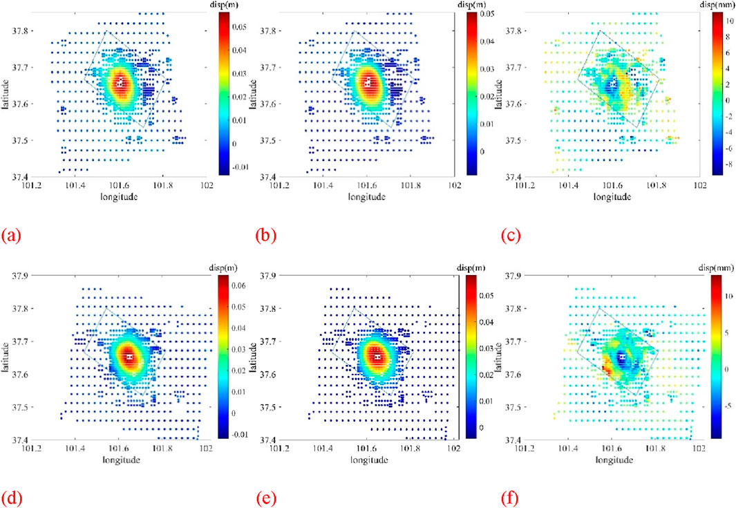
Figure 10. InSAR vs undulating-topography FEM LOS displacements with residuals: 2016 M_W 5.9 Menyuan earthquake. Surface-projected fault traces are delineated by blue polygons. The root mean square error (RMSE) between finite element simulations and InSAR-derived LOS displacements at 1,951 surface observation points is 2.70929434322033 × 10⁻³ m. (a) Ascending LOS displacements (Track AT128) from Sentinel-1A InSAR; (b) Predicted ascending LOS displacements by our finite element model; (c) Residual ascending LOS displacements (Observed–Modeled); (d) Descending LOS displacements (Track DT33) from Sentinel-1A InSAR; (e) Predicted descending LOS displacements by our finite element model; (f) Residual descending LOS displacements (Observed–Modeled).

5 Conclusion

In this study, we introduced a novel method for fault coseismic dislocation inversion using parallel elastic finite element numerical simulation. The validity of this approach was confirmed through two checkerboard tests for fault coseismic dislocation inversion, demonstrating its accuracy and reliability. Building on these results, we applied the proposed method to the 2016 M_W 5.9 earthquake to determine the fault coseismic dislocation distribution. The inversion was conducted using three different techniques: Damped Least Squares Method (DLSM), Smoothed Least Squares Method (SLSM), and the Steepest Descent Method (SDM). The resulting surface coseismic displacement distributions closely matched the InSAR observation data, underscoring the method’s precision and robustness.

The influences of topographic relief and material heterogeneity on coseismic fault dislocation inversions require separate investigation, as their impact magnitudes and mechanisms may differ substantially. The consistency between inversion results and observational data indicates that our method effectively accounts for surface topography variations and medium inhomogeneity, which are critical factors in accurately modeling fault dislocations. This approach leverages the computational power of parallel processing, enabling efficient handling of complex geophysical models and large datasets, thus demonstrating its potential for widespread application in earthquake science. Ideal model tests show that the 10% difference in Young’s modulus between the two sides of the fault has a significanteffect on the coseismic dislocation inversion. For the example of the 2016 Menyuan M_W 5.9 earthquake, topographic relief had a small effect on the coseismic dislocation inversion. In general, the specific effects of medium differences and topographic relief need to be studied individually.

Furthermore, the versatility of the proposed method allows it to adapt to various seismic scenarios, providing a comprehensive tool for researchers and practitioners. By integrating advanced numerical simulation techniques with robust inversion algorithms, this method offers significant improvements over traditional approaches, enhancing our ability to understand and predict seismic events.

In conclusion, the fault coseismic dislocation inversion method based on parallel elastic finite element numerical simulation presents a powerful and adaptable solution for analyzing earthquake-induced displacements. Its ability to incorporate realistic geophysical conditions makes it a valuable asset for advancing seismic research and improving our preparedness for future seismic activities. This work paves the way for further studies to refine and expand the method’s capabilities, contributing to the ongoing development of earthquake science and engineering.

Data availability statement

The original contributions presented in the study are included in the article/supplementary material, further inquiries can be directed to the corresponding authors.

Author contributions

YC: Conceptualization, Data curation, Formal Analysis, Investigation, Methodology, Resources, Software, Validation, Visualization, Writing – original draft. CH: Conceptualization, Data curation, Formal Analysis, Funding acquisition, Investigation, Methodology, Project administration, Resources, Software, Supervision, Validation, Visualization, Writing – original draft, Writing – review & editing. MS: Formal Analysis, Investigation, Methodology, Software, Validation, Visualization, Writing – review & editing. HZ: Conceptualization, Funding acquisition, Investigation, Methodology, Project administration, Resources, Software, Supervision, Writing – original draft.

Funding

The author(s) declare that financial support was received for the research and/or publication of this article. This research was financially supported by the National Key Research and Development Program of China (Grant Nos. 2023YFF0804300, 2023YFF0804301) and National Natural Science Foundation of China (Grant Nos. 42374116).

Acknowledgments

We thank Prof. Yaolin Shi (University of Chinese Academy of Sciences), Yongen Cai (Peking University) for their helpful suggestions. This research was financially supported by the National Key Research and Development Program of China (Grant Nos. 2023YFF0804300, 2023YFF0804301) and National Natural Science Foundation of China (Grant Nos. 42374116).

Conflict of interest

The authors declare that the research was conducted in the absence of any commercial or financial relationships that could be construed as a potential conflict of interest.

Generative AI statement

The author(s) declare that no Generative AI was used in the creation of this manuscript.

Publisher’s note

All claims expressed in this article are solely those of the authors and do not necessarily represent those of their affiliated organizations, or those of the publisher, the editors and the reviewers. Any product that may be evaluated in this article, or claim that may be made by its manufacturer, is not guaranteed or endorsed by the publisher.

References

Allen, D. M. (1974). The relationship between variable selection and data argumentation and a method for prediction. Technometrics 16 (1), 125–127. doi:10.2307/1267500

CrossRef Full Text | Google Scholar

Bagnardi, M., and Hooper, A. (2018). Inversion of surface deformation data for rapid estimates of source parameters and uncertainties: a Bayesian approach. Geochem. Geophys. Geosystems 19 (7), 2194–2211. doi:10.1029/2018gc007585

CrossRef Full Text | Google Scholar

Barba-Sevilla, M., Glasscoe, M. T., Parker, J., Lyzenga, G. A., Willis, M. J., and Tiampo, K. F. (2022). High-resolution finite fault slip inversion of the 2019 Ridgecrest earthquake using 3D finite element modeling. J. Geophys. Res. Solid Earth 127, e2022JB024404. doi:10.1029/2022JB024404

CrossRef Full Text | Google Scholar

Chen, C. W., and Zebker, H. A. (2000). Network approaches to two-dimensional phase unwrapping: Intractability and two new algorithms. J. Opt. Soc. Am. A 17 (3), 401–414. doi:10.1364/josaa.17.000401

PubMed Abstract | CrossRef Full Text | Google Scholar

Chen, Y., Hu, C., and Zhang, H. (2025). Parallel finite element algorithm forlarge elastic deformations: Programdevelopment and validation. Eng 6, 48. doi:10.3390/eng6030048

CrossRef Full Text | Google Scholar

Deo, A. S., and Walker, I. D. (1995). Overview of damped least-squares methods for inverse kinematics of Robot Manipulators. J. lntelligent Robotic Syst. 14, 43–68. doi:10.1007/bf01254007

CrossRef Full Text | Google Scholar

Duan, H., Wu, S., Kang, M., Xie, L., and Chen, L. (2020). Fault slip distribution of the 2015 M_W7.8 Gorkha (Nepal) earthquake estimated from InSAR and GPS measurements. J. Geodyn. 139, 101767. doi:10.1016/j.jog.2020.101767

CrossRef Full Text | Google Scholar

Element Computing Technology Co., Ltd. (2018). Parallel architecture of FELAC. Element computing technology Co., Ltd. Tianjin, China, 8–14.

Google Scholar

Fan, Q., Xu, C., Yi, L., Liu, Y., Wen, Y., and Yin, Z. (2017). Implication of adaptive smoothness constraint and Helmert variance component estimation in seismic slip inversion. J. Geodesy 91 (10), 1163–1177. doi:10.1007/s00190-017-1015-0

CrossRef Full Text | Google Scholar

Freed, A. M. (2005). Earthquake triggering by static, dynamic, and postseismic stress transfer. Annu. Rev. Earth Planet. Sci. 33 (1), 335–367. doi:10.1146/annurev.earth.33.092203.122505

CrossRef Full Text | Google Scholar

Golub, G. H., Heath, M., and Wahba, G. (1979). Generalized Cross-Validation as a method for choosing a good ridge parameter. Technometrics 21 (2), 215–223. doi:10.1080/00401706.1979.10489751

CrossRef Full Text | Google Scholar

Hansen, P. C. (1992). Analysis of discrete ill-posed problems by Means of the L-Curve. SIAM Rev. 34 (4), 561–580. doi:10.1137/1034115

CrossRef Full Text | Google Scholar

Hansen, P. C., and O'leary, D. P. (1993). The Use of the L-curve in the regularization of discrete ill-posed problems. SIAM J. Sci. Comput. 14 (6), 1487–1503. doi:10.1137/0914086

CrossRef Full Text | Google Scholar

Harris, R. A., and Segall, P. (1987). Detection of a locked zone at depth on the Parkfield, California, segment of the san Andreas fault. J. Geophys. Res. 92 (B8), 7945–7962. doi:10.1029/jb092ib08p07945

CrossRef Full Text | Google Scholar

Harris, R. A., and Segall, P. (1987). Detection of a locked zone at depth on the Parkfield, California, segment of the san Andreas fault. J. Geophys. Res. 92 (B8), 7945–7962. doi:10.1029/jb092ib08p07945

CrossRef Full Text | Google Scholar

Helmert, F. R. (1907). Scientific Books: Die Ausgleichungsrechnung Nach der methode der Kleinsten Quadrate[M]. 26(672): 663–664.

Google Scholar

Hong, S., and Liu, M. (2021). Postseismic deformation and afterslip evolution of the 2015 Gorkha earthquake constrained by InSAR and GPS observations. J. Geophys. Res. Solid Earth 126, e2020JB020230. doi:10.1029/2020JB020230

CrossRef Full Text | Google Scholar

Jiang, H., Feng, G., Wang, T., and Burgmann, R. (2017). Toward full exploitation of coherent and incoherent information in Sentinel-1 TOPS data for retrieving surface displacement: application to the 2016 Kumamoto (Japan) earthquake. Geophys. Res. Lett. 44, 1758–1767. doi:10.1002/2016gl072253

CrossRef Full Text | Google Scholar

Jonsson, S. O., Zebker, H., Segall, P., and Falk, A. (2002). Fault slip distribution of the 1999 M_W7.1 Hector Mine, California, earthquake, estimated from satellite radar and GPS measurements. Bull. Seismol. Soc. Am. 92 (4), 1377–1389. doi:10.1785/0120000922

CrossRef Full Text | Google Scholar

Kim, M., So, B., Kim, S., Jo, T., and Chang, S. (2024). Mesh size effect on finite source inversion with 3- D finite-element modelling. Geophys. J. Int. 237 (2), 716–728. doi:10.1093/gji/ggae060

CrossRef Full Text | Google Scholar

King, G. C. P., Stein, R. S., and Lin, J. (1994). Static stress changes and the triggering of earthquakes. Bull. Seismol. Soc. Amer. 84, 935–953. doi:10.1785/BSSA0840030935

CrossRef Full Text | Google Scholar

Landry, W., and Barbot, S. (2016). Gamra: simple meshing for complex earthquakes. Comput. and Geosciences 90, 49–63. doi:10.1016/j.cageo.2016.02.014

CrossRef Full Text | Google Scholar

Langer, L., Beller, S., Hirakawa, E., and Tromp, J. (2023). Impact of sedimentary basins on Green’s functions for static slip inversion. Geophys. J. Int. 232 (1), 569–580. doi:10.1093/gji/ggac344

CrossRef Full Text | Google Scholar

Langer, L., Gharti, H. N., and Tromp, J. (2019). Impact of topography and three-dimensional heterogeneity on coseismic deformation. Geophys. J. Int. 217 (2), 866–878. doi:10.1093/gji/ggz060

CrossRef Full Text | Google Scholar

Leveque, R. J., and Li, Z. (1994). The immersed interface method for elliptic equations with discontinuous coefficients and singular sources. SIAM J. Numer. Analysis 31 (4), 1019–1044. doi:10.1137/0731054

CrossRef Full Text | Google Scholar

Li, S. Y., and Barnhart, W. D. (2020). Impacts of topographic relief and crustal heterogeneity on coseismic deformation and inversions for fault geometry and slip: a case study of the 2015 Gorkha earthquake in the central Himalayan arc. Geochem. Geophys. Geosystems 21, e2020GC009413. doi:10.1029/2020gc009413

CrossRef Full Text | Google Scholar

Li, Y., Jiang, W., Zhang, J., and Luo, Y. (2016). Space geodetic observations and modeling of 2016 M_W 5.9 Menyuan earthquake: Implications on seismogenic tectonic motion. Remote Sens. 8 (6), 519. doi:10.3390/rs8060519

CrossRef Full Text | Google Scholar

Luo, H., and Wang, T. (2022). Strainpartitioning on the western Haiyuanfault system revealed by the adjacent 2016 M_W5.9 and 2022 M_W6.7 Menyuan earthquakes. Geophys. Res. Lett. 49, e2022GL099348. doi:10.1029/2022GL099348

CrossRef Full Text | Google Scholar

Masterlark, T. (2003). Finite element model predictions of static deformation from dislocation sources in a subduction zone: Sensitivities to homogeneous, isotropic, Poisson-solid, and half-space assumptions. J. Geophys. Res. 108, 2540. doi:10.1029/2002JB002296

CrossRef Full Text | Google Scholar

Melosh, H. J., and Raefsky, A. (1981). A simple and efficient method for introducing faults into finite element computations. Bull. Seismol. Soc. Am. 71 (5), 1391–1400. doi:10.1785/bssa0710051391

CrossRef Full Text | Google Scholar

Minato, S., Wapenaar, K., and Ghose, R. (2020). Elastic least-squares migration for quantitative reflection imaging of fracture compliances. Geophysics 85 (6), 327–342. doi:10.1190/GEO2019-0703.1

CrossRef Full Text | Google Scholar

Moreno, M., Melnick, D., Rosenau, M., Baez, J., Klotz, J., Oncken, O., et al. (2012). Toward understanding tectonic control on the M_W8.8 2010 Maule Chile earthquake. Earth Planet. Sci. Lett. 2012 (3), 152–165. doi:10.1016/j.epsl.2012.01.006

CrossRef Full Text | Google Scholar

Niu, J., Xu, C., and Fan Q& Yin, Z. (2016). Impact of coseismic deformation fields with different time scales on finite fault modelling in 2010 California Baja Earthquake. Surv. Rev. 48 (347), 94–100. doi:10.1179/1752270614y.0000000148

CrossRef Full Text | Google Scholar

Okada, Y. (1992). Internal deformation due to shear and tensile faults in a half-space. Bull. Seismol. Soc. Am., 82(2):1018–1040. doi:10.1785/bssa0820021018

CrossRef Full Text | Google Scholar

Ozawa, S., Nishimura, T., Suito, H., Kobayashi, T., Tobita, M., and Imakiire, T. (2011). Coseismic and postseismic slip of the 2011 magnitude-9 Tohoku-Oki earthquake. Nature 475 (7356), 373–376. doi:10.1038/nature10227

PubMed Abstract | CrossRef Full Text | Google Scholar

Quiroz, E. A. P., Quispe, E. M., and Oliveira, P. R. (2008). Steepest descent method with a generalized Armijo search for quasiconvex functions on Riemannian manifolds. J. Math. Anal. Appl. 341, 467–477. doi:10.1016/j.jmaa.2007.10.010

CrossRef Full Text | Google Scholar

Ragon, T., and Simons, M. (2021). Accounting for uncertain 3-D elastic structure in fault slip estimates. Geophys. J. Int. 224 (2), 1404–1421. doi:10.1093/gji/ggaa526

CrossRef Full Text | Google Scholar

Ramirez-Guzman, L., and Hartzell, S. (2020). 3-D joint geodetic and strong-motion finite fault inversion of the 2008 May 12 Wenchuan, China Earthquake. Geophys. J. Int. 222 (2), 1390–1404. doi:10.1093/gji/ggaa239

CrossRef Full Text | Google Scholar

Rollins, C., Avouac, J.-P., Landry, W., Argus, D. F., and Barbot, S. (2018). Interseismic strain accumulation on faults beneath Los Angeles, California. J. Geophys. Res. Solid Earth 123, 7126–7150. doi:10.1029/2017JB015387

CrossRef Full Text | Google Scholar

Shi, M., Meng, S., Hu, C., and Shi, Y. (2023). Crustal heterogeneity effects on coseismic deformation: numerical simulation of the 2008 M_W 7.9 Wenchuan earthquake. Front. Earth Sci. 11, 1245677. doi:10.3389/feart.2023.1245677

CrossRef Full Text | Google Scholar

Stein, R. S. (1999). The role of stress transfer in earthquake occurrence. Nature 402 (6762), 605–609. doi:10.1038/45144

CrossRef Full Text | Google Scholar

Tikhonov, A. N. (1963). Solution of incorrectly formulated problems and the regularization method. Sov. Math. Dokl. 4, 1035–1038.

Google Scholar

Tilmann, F., Zhang, Y., Moreno, M., Saul, J., Eckelmann, F., Palo, M., et al. (2016). The 2015 Illapel earthquake, central Chile: a type case for a characteristic earthquake? Geophys. Res. Lett. 43, 574–583. doi:10.1002/2015GL066963

CrossRef Full Text | Google Scholar

Wan, Y., Shen, Z.-K., Bürgmann, R., Sun, J., and Wang, M. (2017). Fault geometry and slip distribution of the 2008 M_W 7.9 Wenchuan, China earthquake, inferred from GPS and insar measurements. Geophys. J. Int. 208, 748–766. doi:10.1093/gji/ggw421

CrossRef Full Text | Google Scholar

Wang, K., and Fialko, Y. (2018). Observations and modeling of coseismic and postseismic deformation due to the 2015 M_W7.8 Gorkha (Nepal) earthquake. J. Geophys. Res. Solid Earth 123, 761–779. doi:10.1002/2017JB014620

CrossRef Full Text | Google Scholar

Wang, R., Schurr, B., Milkereit, C., Shao, Z., and Jin, M. (2011). An improved automatic scheme for empirical baseline correction of digitalstrong-motion records. Bull. Seismol. Soc. Am. 101 (5), 2029–2044. doi:10.1785/0120110039

CrossRef Full Text | Google Scholar

Wang, T., and Jonsson, S. (2015). Improved SAR amplitude image offset measurements for deriving three-dimensional coseismic displacements. IEEE J. Sel. Top. Appl. Earth Observations Remote Sens. 8 (7), 3271–3278. doi:10.1109/jstars.2014.2387865

CrossRef Full Text | Google Scholar

Wang, T., Jonsson, S., and Hanssen, R. F. (2014). Improved SAR image coregistration using pixel-offset series. IEEE Geoscience Remote Sens. Lett. 11 (9), 1465–1469. doi:10.1109/lgrs.2013.2295429

CrossRef Full Text | Google Scholar

Williams, C. A., and Wallace, L. M. (2018). The impact of realistic elastic properties on inversions of shallow subduction interface slow slip events using seafloor geodetic data. Geophys. Res. Lett. 45, 7462–7470. doi:10.1029/2018GL078042

CrossRef Full Text | Google Scholar

Xu, G., Xu, C., Wen, Y., and Yin, Z. (2019). Coseismic and postseismic deformation of the 2016 M_W 6.2 Lampa earthquake, southern Peru, constrained by interferometric synthetic aperture radar. J. Geophys. Res. Solid Earth 124, 4250–4272. doi:10.1029/2018jb016572

CrossRef Full Text | Google Scholar

Zhang, Y., Feng, W., Chen, Y., et al. (2012). The 2009 L’Aquila M_W 6.3 earthquake: a new technique to locate the hypocentre in the joint inversion of earthquake rupture process. Geophys. J. Int. 191, 1417–1426. doi:10.1111/j.1365-246X.2012.05694.x

CrossRef Full Text | Google Scholar

Zhang, Y., Shan, X., Zhang, G., Zhong, M., Zhao, Y., Wen, S., et al. (2020). The 2016M_W 5.9 Menyuan earthquake in the Qilian orogen, China: a potentially delayed depth-segmented rupture following from the 1986 M_W6.0 Menyuan earthquake. Seismol. Res. Lett. 91 (2A), 758–769. doi:10.1785/0220190168

CrossRef Full Text | Google Scholar

Zhang, Y., Wang, R., Yun-tai, C. Y., Xu, L., Du, F., Jin, M., et al. (2014). Kinematic rupture model and Hypocenter Relocation of the 2013 M_W 6.6 Lushan earthquake constrained by strong-motion and Teleseismic data. Seismol. Res. Lett. 85 (1), 15–22. doi:10.1785/0220130126

CrossRef Full Text | Google Scholar

Zuo, R. H., Qu, C. Y., Shan, X. J., Zhang, G. H., and Song, X. G. (2016). Coseismic deformation fields and a fault slip model for the M_W7.8 mainshock and M_W7.3 aftershock of the Gorkha-Nepal 2015 earthquake derived from Sentinel-1A SAR interferometry. Tectonophysics 686, 158–169. doi:10.1016/j.tecto.2016.07.032

CrossRef Full Text | Google Scholar