A new three-dimensional mesh modeling method for geological bodies containing complex faults in geological engineering

Three-dimensional geological modeling and visualization hold considerable significance for both application and research across various fields, including geosience, marine geology, environmental protection, mining engineering, and geological engineering. However, the technique and approach are exposed to critical challenges for complex geological bodies, including heightened structural complexity, extensive manual intervention, and diminished accuracy of discontinuity surfaces owing to the presence of faults, particularly conflicting discontinuity surfaces generated by reverse faults. In this paper, a novel technical workflow and a set of three-dimensional structure modeling methods for geological bodies containing complex faults were designed. A model stitching strategy based on the ear clipping algorithm was proposed to incorporate fine fault models into the modified original model. This strategy transforms the integration of complex three-dimensional models into a triangulation problem for simple two-dimensional polygons, ensuring topologically consistent and computationally efficient merging. Simultaneously, a contour line segments sorting algorithm based on a vertex sequence was proposed to accelerate the extraction of boundary contour line segments. We used a two-stage detection strategy to accelerate locating overlap regions. A multi-layer triangulated irregular network-3DT model was constructed through continuous stratum modeling, fine fault modeling, overlap detection based on the two-dimensional projection topological relationship, extraction of ordered contour line segments of model boundaries, and model reconstruction based on the ear clipping. An underground modeling experiment revealed that these modeling methods and technical systems can accurately depict the geometric form around complex geological faults. A quantitative and qualitative comparison between the proposed modeling method and various modeling methods demonstrates that our method is superior in flexibility, robustness, and mesh quality.

1 Introduction

Land-based mining is crucial for resource supply, economic development, employment stability, and national strategic security. Meanwhile, deep-sea mining, as a new resource source, drives technological innovation and industrial upgrading. Ensuring efficient, safe, and sustainable mining of underground resources merits in-depth research. Three-dimensional geological modeling can effectively integrate data from different professions, periods, sources and types and establish a multi-source data warehouse (Zhang et al., 2010). Moreover, the digital modeling and representation of rock masses and reservoirs can infer present the distribution of underground mineral resources and the geological structure in the mining area and can also be used as a basic model for studying the characteristics of strata deformation and support methods for controlling strata. Clearly presenting gas hydrates and landslide high-risk zones can support accurate assessment and safety monitoring. Virtual trial-and-error construction schemes for underground and offshore systems can optimize engineering design and construction. Therefore, three-dimensional geological modeling technology can provide technical support for risk assessment, numerical simulation, strata support, and personnel safety protection during mining to promote the safe, reasonable and efficient mining of ore, coal, oil and gas, and groundwater resources.

Three-dimensional geological modeling primarily involves feature- and field-based modeling (Jessell, 2001). Feature-based modeling focuses on generating a structure or vector model in three dimensions by using geological space data, and the geological properties are currently assumed to be homogeneous (Zhang et al., 2010). In reservoir development and evaluation research, significant attention is given to geological attributes such as porosity, temperature fields, and stress fields. For such purposes, data-field modeling and uncertainty modeling are particularly suitable. Additionally, field-based modeling techniques can be effectively employed to model ore bodies and layered interfaces (Zhong et al., 2021).

Several scholars have contributed to such studies, and reported significant achievements (Trubetskoy et al., 2012; Zhong et al., 2007; Frank et al., 2007; Jun-Qi et al., 2013). Common spatial data structures, including 2.5D and 3D structures, are classified into surface, volume, and hybrid data structures. Surface-based data structures include grids, shape, facets, boundary representation (B-Rep), and section (Tipper, 1976; Ming et al., 2010); volume-based data structures include 3D arrays, Block, needle, Octree, constructive solid geometry (CSG), tetrahedral network (TEN), triangular prism (tri-prism) and its extensions generalized tri-prism (GTP) (Wu 2004); and hybrid spatial data structures include T-splines-NURBS-B-Rep, Octree + CSG, multi-layer digital elevation model (multi-DEM) method, and WireFrame + Block. In general, owing to the concise topological relationship, the surface element model requires less storage space and performs better in space vector operations. Moreover, the voxel model is more suitable for non-uniform property field calculations, process simulations and reserve calculations. Many studies have demonstrated that surface models can be transformed into a voxel mesh models (Tertois and Mallet, 2007; Xiang-bin et al., 2010). The authors of Liu et al. (2012) integrated a similar tri-prism model with the traditional multi-layer triangular irregular network (TIN) model. Article (Zhang Z. et al., 2018) implemented the conversion of the surface-based models to TEN, and clearly describeed the internal structure and the non-uniform attribute field of the geological body.

Different methods are typically used to infer and simulate complex geological structures and phenomena such as macro-stratification, local intrusion, folding, faulting, and lenses. Subsequently, these complex geological structures were integrated through processes such as trimming, connecting, and incorporating expert knowledge-driven operations to obtain a complete geological body model. This study focuses on accurately and automatically describing the geometry of geological bodies and geological structures; therefore the mesh-geological-interface-based modeling methods are adopted.

For continuous geological structures, intrusion surfaces, and multi-valued surfaces formed by intrusion, inversion, and folding, both NURBS surfaces and implicit modeling methods are relatively effective, and implicit modeling methods have a higher degree of automation (Guo et al., 2018; Zhong et al., 2019b, Zhong et al., 2019a; Hillier et al., 2014). In recent years, neural network-based methods have been increasingly applied in the identification of geological structures (Guo et al., 2021; Chai and Maceira, 2022; Yang et al., 2022). A large amount of annotated earthquake data and borehole data are used to train neural network models (Liu et al., 2024; Lin et al., 2025). Faults are complex and common geological structures that are generated after strata fracture and displacement deformation. Coal seam rockburst in fault zones has gradually become one of the most dangerous disasters in coal mining in recent years. The prevention and control of coal seam rockburst in fault zones has become a critical challenge, with significant economic and social impacts. Under the action of tectonic compression, reverse faults, which are often sites of oil and gas accumulation, form overlapping areas. Therefore, the triangularization of reverse faults has practical application significance for oil and gas exploration technology. Moreover, the mechanical characteristics, stress changes, and other properties at discontinuous points in the model are more complex than those at continuous points. The accuracy of the fault location and shape has a significant impact on the results of the numerical simulation calculations. Therefore, the geometric modeling of faults has always been a research hotspot. Using a certain type of data alone cannot completely and accurately describe the geometric structure of geological objects in a complex geological environment, especially complex geological bodies with reverse faults. The interactive use of multi-source data can provide more details of geological objects for modeling to achieve better application significance and visual effects.

Fault lines, stratum pinch-out lines and regional boundaries can be used as zoning basis and constraint information (Che and Jia, 2019; Jia et al., 2020). The mesh-based model interpolates according to the fault location and combines the corresponding single value plane. In addition, the virtual zoning method sets the direction of the fault line to segment and constrain the modeling region to which the breakpoint belongs. Another commonly used method is the clipping technique based on triangular meshes and geometric calculations. Geological modeling methods based on stratum recovery (Zhu et al., 2006; Wu and Xu, 2003; Wu et al., 2005) find intersecting lines between the stratum surface and fault surface, and then move up and down the upthrown and downthrown intersections according to the fault displacement. Meng et al. applied triangulated irregular network and tetrahedral network to model complex geological objects (Xiang-bin et al., 2010). Jia et al. moved the intersection line of a fault according to the displacement and reconstructed the mesh surface according to the corresponding boundary and interline (Jia et al., 2019). Similarly, Boolean operations based on surfaces and volumes are often used for fault modeling. Guo et al. used boundary lines and attitudes to construct various geological interfaces, and performed Boolean operations on the basic body model to simulate complex geological bodies (Guo et al., 2016). Song et al. embedded fault polyhedrons created by the makefaces plug-ins and push-pull and drawing tools into a continuous simple geological body model through Boolean operations (Song et al., 2019). Experts analyze, compare, and integrate various types of data to fully leverage these records. Additionally, on the basis of the fusion of multi-source data (Kaufmann and Martin, 2009; Wu and Xu, 2014), extrapolating and calculating more data according to structural plane characteristics also helps in modeling (Wu et al., 2015). Sterlacchini and Zanchi reconstructed structural surfaces by interpolating linear elements obtained by projection and down-dip plunge, superficial traces of the structures, and 2-D sections (Sterlacchini and Zanchi, 2003). Another frequently used modeling strategy is to divide modeling units according to fault location and interpolate both sides of the fault. The GTP and parametric geological models (Zhang Y. et al., 2018; Lyu et al., 2021) have been introduced into modeling of complex geological bodies.

Among these current methods of dealing with faults; Some modeling methods based on the subareas division make full use of fault line information to describe faults in detail; however, in some cases, it is also difficult to reasonably divide areas containing multiple faults with complex intersectant relationships. Boolean operation, intersecting operation and projection polyline control cannot precisely describe the elevation of the hanging wall and footwall for reverse faults. The later movement of the intersections on the hanging wall and footwall data of faults can produce better results but require significant user intervention and computation. Some modeling methods based on the subareas division make full use of fault line information to describe faults in detail; however, in some cases, it is also difficult to reasonably segmenting areas containing multiple faults with complex intersectant relationships is difficult. Additionally, when the data satisfy certain requirements, the method based on the GTP model can complete the modeling. Although NURBS and its enhanced method eliminate the need for mesh transformation, they still require calculation and adjustment of the corresponding control point positions following the cutting process.

After studying and analyzing the currently prevalent methods, we identify that there are three problems that require further research and solutions: (1) Finding simple methods to accurately express the geometry of the hanging wall and footwall within the range of fault influence; (2) Eliminating manual intervention caused by calculation and movement of each points on fault lines while ensuring the implementation of (1); (3) Ensuring the quality of the triangular mesh on the reconstructed plane as much as possible When correctly reconstructing and combining the geological interface. Therefore, this paper describes a new and complete framework for the 3D representation and modeling of complex geological bodies. This study attempts to directly generate the intersection lines of the fault and coal seam, and the hanging wall and footwall surface within the range of influence of the fault according to the spatial data. If geological map data are used directly for modeling, the approach is relatively more accurate than the later processing. Because of the low number of boreholes, fault information is limited, and several studies used section maps to generate 3D models of complex geological structures (Lemon and Jones, 2003; Qu et al., 2006; He et al., 2008). We developed more accurate models by extracting the hanging wall and footwall surface data of the faults from the multi-source data to replace the rough parts of the original model. We introduced an ear clipping algorithm (Mei et al., 2012) into the modeling of geological bodies to ensure compatibility and transition with the two-dimensional projection topological relationship of TINs. In addition, we proposed a new contour line segments sorting algorithm based on a vertex sequence to aid modeling. The new contour line segments sorting algorithm has the advantages of easy implementation, high reusability, and requiring low storage requirements. In our modeling process, many algorithms were used to improve the automation of the modeling; these algorithms include the triangular mesh generation, collision detection, boundary contour extraction, contour line segments sorting, and reconstruction algorithms for triangulating surfaces between boundary contour line segments. Implementing this algorithm is an indispensable auxiliary step in cutting and splitting, rapid slicing, and fast intersection algorithms.

The rest of this paper is organized as follows. First, we summarize the main principle and implementation of the modeling approach used in this study. Next, we describe the entire modeling process and algorithms used by our modeling approach and provide the details of the proposed algorithm. Then, the details of the data and results from the modeling experiments are described. Subsequently, a quantitative and qualitative comparison between the proposed modeling method and various representative automatic and semi-automatic modeling methods is presented. Finally, some concluding remarks are reported.

2 Methodology

2.1 The fundamental principles and overall framework of our method

We regarded complex geological bodies as a combination of a series of strata interfaces and fault surfaces to generate a 3DT geological model based on the geological structures. The newly proposed modeling principles and workflow are shown in Figure 1.

Figure 1

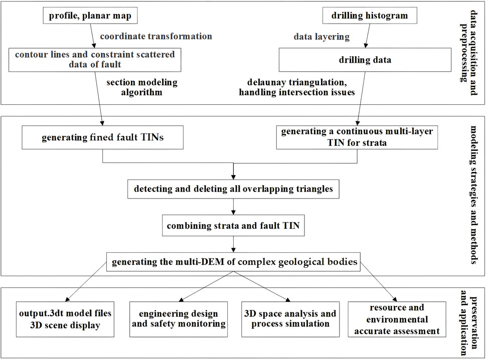
Figure 1. The new workflow of 3D geological modeling.

The main steps and some formal definitions are as follows:

1. Data processing stage, geological map data are extracted and preprocessed to prepare for modeling. We obtained section lines and constraint scattered data of fault from profile and planar map by coordinate calibration and transformation, and drilling data from drilling histogram by data layering.

2. Modeling stage, First, the triangular mesh surfaces (symbolized as I) of the strata are generated using borehole data; fault models containing upper and lower wall (symbolized as I_F) and fault surfaces (symbolized as S) within the range of influence of the fault are generated using contour lines and constraint scattered data. It may be possible to obtain overlapping stratum data at a certain borehole. Therefore, when generating a continuous stratum surface model based on the restoration theory, the overlapping information is usually removed. Subsequently, all triangles conflicting with a fault model are deleted to obtain a stratigraphic triangular mesh surface with an inner hole whose boundary data are considered to be reliable. A certain error was observed between the triangulated irregular network surface generated by the rest of the drilling data and the real hanging wall and footwall fault surface. This study removed all possible errors. Subsequently, the triangulation network between the boundary of the inner hole and the boundary of the fault model is reconstructed. Finally, each fault is cyclically processed to obtain a complete fine stratum model of each layer, and all fault surfaces are embedded.

3. Model preservation and application stage, models are commonly used for engineering design and safety monitoring, resource and environmental accurate assessment, 3D space analysis and numerical simulation, and 3D scene display.

2.2 The topological structure and storage of model

We stored and processed the data in an object-oriented manner in .3dt files. The geological body data model in this study includes point objects, triangular facet objects, TIN surface objects and multi-DEM objects. The data structure and topology relationships are simple and occupy less storage space. The points storing specific coordinate information belong to the triangular facet, and the triangular facets constitute the TIN surface model with triangular facet numbers. The multiple TIN faces are combined to obtain the multi-DEM. The data points forming the triangles are stored counterclockwise. In addition, the complex topological relationships of modeling such as edges and adjacency relationships can be derived from this basic data structure. Let Model be a set consisting of all mesh surfaces: $\mathrm{M}\mathrm{o}\mathrm{d}\mathrm{e}\mathrm{l}=\{{\mathrm{I}}^{\prime },{\mathrm{I}}_{\mathrm{F}},\mathrm{S},\mathrm{G}\}$ and surface ${\mathrm{I}}^{\prime }$ is obtained through a series of operations on surface I. Surface G is a mesh generated during our workflow. $\forall \alpha \in \mathrm{M}\mathrm{o}\mathrm{d}\mathrm{e}\mathrm{l},{\mathrm{M}}_{\alpha }=({\mathrm{V}}_{\alpha },{\mathrm{E}}_{\alpha },{\mathrm{T}}_{\alpha })$, ${\mathrm{V}}_{\alpha }=\{v_{\alpha 1},v_{\alpha 2},\dots ,v_{\alpha m_{\alpha }}\},{\mathrm{T}}_{\alpha }=\{t_{\alpha 1},t_{\alpha 2},\dots ,t_{\alpha n_{\alpha }}\}$, ${\mathrm{E}}_{\alpha }=\{e_{\alpha 1},e_{\alpha 2},\dots ,e_{\alpha k_{\alpha }}\}$ is inferred from ${\mathrm{T}}_{\alpha }$, and $\forall \alpha \ne \beta ,{\mathrm{T}}_{\alpha }\cap {\mathrm{T}}_{\beta }=\varnothing$. The 3DT model developed by our team is the backbone of Languang’s geographic information system (LK LionKing), powering support from mine digitization to real-time safety alerts for numerous geoengineering projects. The data objects and structures of its non-geological models are shown in Figure 2.

Figure 2

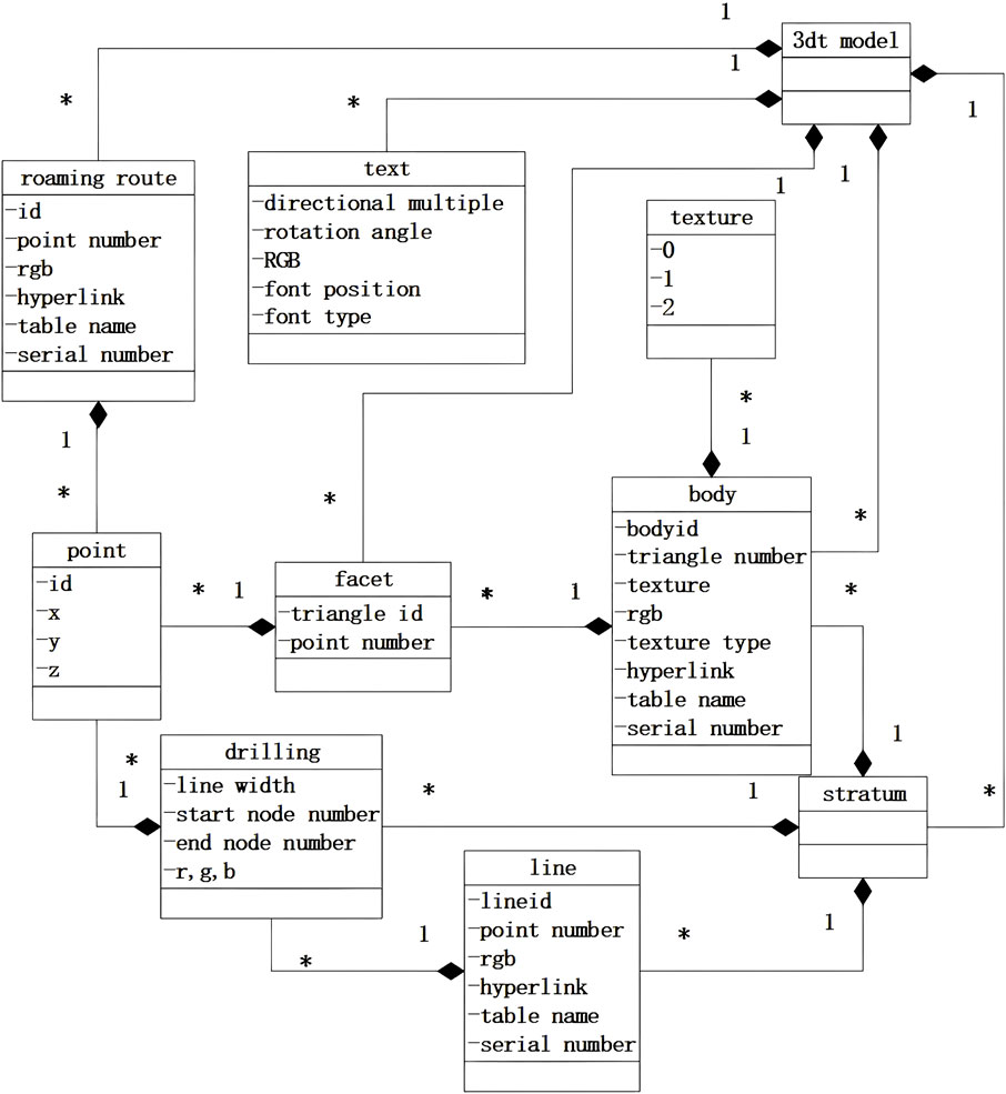
Figure 2. The topological structure of 3DT model.

2.3 Generating the initial continuous stratum model and fine fault models

2.3.1 The initial continuous stratum model

The geometric shapes and structures of geological surfaces are effectively described with TINs by organizing the raw borehole measurements. TINs serve as the carriers for reconstructing and visualizing models for various scattered point interpolation algorithms and implicit modeling methods. We used measured borehole data to generate an initial continuous stratum model and organize the scattered data to display the geometric shape and structure of geological surfaces with triangular meshes. Sibson proved that a Delaunay triangulation can produce an overall optimal triangular mesh for any scattered data and minimize the number of pathological triangles; thus, we generated TINs (Tucker et al., 2001) using the Delaunay triangulation algorithm (Biniaz and Dastghaibyfard, 2012).

Therefore, the triangular mesh of the layer surface $\mathrm{I}$ satisfies the following conditions:

${\mathrm{T}}_{\mathrm{I}}={\mathcal{T}}_{\mathrm{delaunay}}=\left\{\mathrm{t}=⟨{\mathrm{p}}_{\mathrm{i}},{\mathrm{p}}_{\mathrm{j}},{\mathrm{p}}_{\mathrm{k}}⟩\in {\mathcal{P}}^3|\begin{array}{cc}\hfill & 1.\text{conv}(\mathrm{t})\text{is}\hspace{0.17em}\text{a}\hspace{0.17em}\text{simplex}\hspace{0.17em}\text{of\hspace{0.17em}}\hspace{0.17em}\text{the}\hspace{0.17em}\text{Delaunay}\hspace{0.17em}\text{boundary},\hfill \\ \hfill & 2.\forall \mathrm{p}\in \mathcal{P}\backslash \{{\mathrm{p}}_{\mathrm{i}},{\mathrm{p}}_{\mathrm{j}},{\mathrm{p}}_{\mathrm{k}}\},\mathrm{p}\notin \text{Int}(\mathrm{C}(\mathrm{t})),\hfill \\ \hfill & 3.\nexists {\mathcal{T}}^{\prime }\in \mathrm{\Pi }(\mathcal{P})\text{such}\text{that}\underset{{\mathrm{t}}^{\prime }\in {\mathcal{T}}^{\prime }}{\min }{\mathrm{\theta }}_{\min }({\mathrm{t}}^{\prime })>\underset{\mathrm{t}\in {\mathcal{T}}_{\mathrm{D}}}{\min }{\mathrm{\theta }}_{\min }(\mathrm{t})\hfill \end{array}\right\}$

Where $\text{conv}(\mathcal{P})$ represents the global convex hull, and $\text{conv}(\mathrm{t})$ represents the local convex hull of a triangle. $\mathrm{\Pi }(\mathcal{P})$ is the set of all possible valid triangulations on the scatter set $\mathcal{P}$. Int (C(t)) refers to the interior of the circumcircle of t. ${\mathcal{T}}_{\mathrm{delaunay}}$ represents performing triangulation based on delaunay algorithm on a dataset. ${\mathrm{T}}_{\mathrm{I}}$ represents the set of triangles in layer $\mathrm{I}$.

Many algorithms can implement a Delaunay triangulation on scattered points, the Bowyer-Watson algorithm is the most common method that performs well. This algorithm is a “reconnection” method based on the circumcircle property (Rebay, 1993), with the main steps outlined in the Appendix. We used this algorithm to establish a TIN for stratigraphic layer $\mathrm{I}$.

2.3.2 The fine fault models

The fault plane can be expressed in many forms, such as a single plane, a single curved surface, or a splicing surface of multiple curved surfaces (Wu and Xu, 2003; Renard and Courrioux, 1994). For the unified expression and storage of geological data and geometric models, the hanging wall and footwall surfaces of the faults within a certain range and the fault planes were represented by a series of triangular meshes. We extracted data from the sections and used the contour line triangulation reconstruction algorithm to generate fault planes and the hanging wall and footwall surfaces of the fault. The fault planes and the hanging wall and footwall surfaces of the faults in the sections were all single arcs; thus the two contour lines could be stitched together in the form of triangles using the basic algorithms, such as the shortest diagonal method (Liu et al., 2003), the largest volume method (Keppel, 1975), the cut-and-sew method and surface area minimization (Fuchs et al., 1977). The triangles on surface S and I_F can be obtained:

${\mathrm{T}}_{\mathrm{S}}={\mathcal{T}}_{\mathrm{\text{sections}}}\left({\mathrm{V}}_{\mathrm{S}}\right),{\mathrm{T}}_{{\mathrm{I}}_{\mathrm{F}}}={\mathcal{T}}_{\mathrm{sections}}\left({\mathrm{V}}_{{\mathrm{I}}_{\mathrm{F}}}\right).$

${\mathcal{T}}_{\mathrm{sections}}$ denotes the application of the contour line triangulation reconstruction algorithm to the corresponding single-arc pairs on the $\mathrm{S}$ and ${\mathrm{I}}_{\mathrm{F}}$ surfaces.

In fact, all the exploration data and drilling data can be used as supplementary data for modeling. When more reliable data are used for modeling, the geometric characteristics can be expressed more precisely and accurately. When new data become available, we can retriangulate the triangular mesh in the current data models by using a point-by-point insertion triangulation method. For complex intersecting faults, the fault models are processed as a whole to replace the triangles of the original layer, thereby avoiding the loss of the fault information.

2.4 Overlap detection based on the two-dimensional projection topological relationship of model

Although the two triangular faces do not intersect in the three-dimensional form, there may still be a conflict in elevation. Our goal was to remove the overlapping parts of the elevation value; therefore, an overlap test was performed on a two-dimensional projection. Two cases of conflicting triangular faces between the two models: (1) the three vertices of the triangle are inside or on the boundary of the precise model area; (2) at least one point of the three vertices of the triangle was outside the precise model area. If a triangle satisfies any of these cases, it is considered to be overlapping. The set of overlapping triangles is denoted by ${\mathrm{T}}_{\mathrm{overlap}}$. The bounding box and spatial subdivision techniques work efficiently to drastically reduce the number of intersecting pairs that need to be further verified accurately for collision detection. This significantly reduces the computational cost produced by the O$({\text{n}}^2)$ complexity for large-scale engineering problems. The method for constructing an axis-aligned bounding boxe (AABB) is simple, the required storage is small, and the complexity of the intersection test is low. If the computational efficiency is further improved, index structures, such as AABB tree and oriented bounding box (OBB) tree, can be builded. In this manner, many disjoint triangles can be eliminated, thereby bypassing exact intersecting operations through a space search.

To reduce computational complexity, a two-stage detection strategy for locating an approximate overlap region was used. First, we obtained a candidate set of overlapping triangles and overlapping points using AABBs; then accurately verified them in 2D by using the PNPoly algorithm (Walker and Snoeyink, 1999) and an intersection operation. The process is as follows:

1. Calculate a bounding box $\mathrm{B}\mathrm{F}$ for I_F. Calculate the bounding box set $\mathrm{B}$ for all the triangular faces in an $\mathrm{I}$. $\mathrm{B}\mathrm{F}=\left(\left[{\mathrm{x}}_{\min },{\mathrm{x}}_{\max }\right],\left[{\mathrm{y}}_{\min },{\mathrm{y}}_{\max }\right]\right)$; $\mathrm{B}=\left\{{\mathrm{b}}_{\mathrm{i}}=\left(\left[{{\mathrm{x}}_{\min }}^{(\mathrm{i})},{\mathrm{x}}_{\max }^{(\mathrm{i})}\right],\left[{{\mathrm{y}}_{\min }}^{(\mathrm{i})},{\mathrm{y}}_{\max }^{(\mathrm{i})}\right]\right)\mid {\mathrm{t}}_{\mathrm{i}}\in {\mathrm{T}}_{\mathrm{I}}\right\}$.

2. Find all candidate points: CA = {v_j ∈ V_I ∣ (x_min < π_xy (v_j).x < x_max ∧ y_min < π_xy (v_j).y < y_max)}. ${\mathrm{\pi }}_{\mathrm{x}\mathrm{y}}(\cdot )$ is the projection function onto the XY-plane.

3. Find all candidate triangles:

$\mathrm{T}\mathrm{A}=\left\{{\mathrm{t}}_{\mathrm{i}}\in {\mathrm{T}}_{\text{I}}\mid \left({\mathrm{x}}_{\min }^{(\mathrm{i})}\le {\mathrm{x}}_{\max }\wedge {\mathrm{x}}_{\max }^{(\mathrm{i})}\ge {\mathrm{x}}_{\min }\right)\wedge \left({\mathrm{y}}_{\min }^{(\mathrm{i})}\le {\mathrm{y}}_{\max }\wedge {\mathrm{y}}_{\max }^{(\mathrm{i})}\ge {\mathrm{y}}_{\min }\right)\right\}$

4. Find all precise points:

A = {${\mathrm{v}}_{\mathrm{j}}\in \mathrm{C}\mathrm{A}\mid ({\sum }_{\mathrm{e}\in \mathrm{\partial }\mathrm{B}}\mathbb{I}(\exists \mathrm{\lambda }\in (0,\mathrm{\infty }),\exists \mathrm{\mu }\in [\mathrm{0,1}],{\mathrm{\pi }}_{\mathrm{x}\mathrm{y}}({\mathrm{v}}_{\mathrm{j}})+\mathrm{\lambda }\vec{\mathrm{d}}=$$\mathrm{\mu }{\mathrm{e}}_{\mathrm{s}}+\left(1-\mathrm{\mu }\right){\mathrm{e}}_{\mathrm{t}}))\text{mod}2\equiv 1$}$,\text{while:}\vec{\mathrm{d}}=\left(\mathrm{1,0}\right) \text{is} \text{the} \text{direction} \text{of} \text{a}$$\text{horizontal\hspace{0.17em}right}-\text{pointing\hspace{0.17em}ray}{\mathrm{e}}_{\mathrm{s}},{\mathrm{e}}_{\mathrm{t}}\text{is}\text{endpoint}\text{of}\mathrm{e}$. $\mathbb{I}(\cdot )$ is indicator function:

$\mathbb{I}\left(\text{condition}\right)=\left\{\begin{array}{cc}1,\hfill & \text{if\hspace{0.17em}\hspace{0.17em}the\hspace{0.17em}\hspace{0.17em}condition\hspace{0.17em}\hspace{0.17em}is\hspace{0.17em}\hspace{0.17em}true}\hfill \\ 0,\hfill & \text{otherwise}\hfill \end{array}\right.$

5. Find and delete all overlapping triangles for $\mathrm{I}$. ${\mathrm{T}}_{\text{overlap}}=\left\{{\mathrm{t}}_{\mathrm{i}}\in {\mathrm{T}}_{\mathrm{I}}\mid \exists {\mathrm{v}}_{\mathrm{j}}\in \mathrm{A},{\mathrm{t}}_{\mathrm{i}}\in \mathrm{T}\mathrm{A}\right\}$, ${\mathrm{T}}_{{\mathrm{I}}^{\prime }}={\mathrm{T}}_{\mathrm{I}}\backslash \{{\mathrm{t}}_{\mathrm{i}}\in \mathrm{T}\mathrm{A}\mid {\mathrm{t}}_{\mathrm{i}}\cap \mathrm{a}\ne \varnothing ,\mathrm{a}\in \mathrm{A}\}$.

2.5 Generating topologically ordered contour line segments

2.5.1 The contour line segments extraction algorithm for any irregular triangulated surfaces

We obtained a triangular mesh with a cavity after deleting unreliable conflict triangles. We used a simple algorithm suitable for any triangulated irregular network to extract the outer boundary contour line segments of the conflict triangles set and the stratum plane in the fault model, respectively. For a given triangulated irregular network containing a set of triangles, we iterated through all triangle data and recorded the number of occurrences of each edge. When the edge of the triangle appears only once in the entire TIN, it is identified as the target contour line. The number of points belonging to the edge is then recorded. At this point, the contour lines data we obtained are a set of disordered line segments that needed to be sorted before they could be used further. Let Contour denote the contour line segments extraction operator, and $\mathit{f}$ is an edge frequency statistics function:

$f:\mathrm{e}\to \mathbb{N},f\left(\mathrm{e}\right)={\displaystyle \sum _{{\mathrm{t}}_{\mathrm{i}}\in \mathrm{T}}}\mathbb{I}\left(\mathrm{e}\in {\mathrm{t}}_{\mathrm{i}}\right);$

$\mathrm{C}\mathrm{o}\mathrm{n}\mathrm{t}\mathrm{o}\mathrm{u}\mathrm{r}:\mathrm{T}\to \mathrm{L},\mathrm{L}=\mathrm{C}\mathrm{o}\mathrm{n}\mathrm{t}\mathrm{o}\mathrm{u}\mathrm{r}\left(\mathrm{T}\right)=\bigcup _{{\mathrm{t}}_{\mathrm{i}}\in \mathrm{T}}\left\{{\mathrm{e}}_{\mathrm{i}}\in {\mathrm{t}}_{\mathrm{i}}\mid f\left({\mathrm{e}}_{\mathrm{i}}\right)=1\right\}.$

2.5.2 The contour line segments sorting algorithm

The adjacency relationships of triangles or the topological relationships between intersections, edges and facets can be used to order the intersections into continuous line segments (Lo and Wang, 2004; Hua et al., 2006; Dianzhu et al., 2009). Sun Dianzhu et al. used an improved tree ${\text{R}}^{*}$ to build a spatial index structure for intersection segments and then constructed chains/loops using this indexing and distance relationship. The above methods are compatible with the methods and data structures that deal with practical problems. However, many topologies and affiliations need to be stored and searched. Compared with these algorithms, the method of using a hash table only needs to consider the point coordinates at both ends of the intersection line segment. The hash table uses a dynamic search mechanism to track the line segments. The processing method is simple; however, if the span of the vertex coordinates is too large, the choice of the hash function and conflict resolution methods is a challenging.

Based on the actual problems and context algorithms presented in this article, we used a dynamic sorting process to connect the contour line segments end-to-end. We transformed the sorting of line segments into sorting points pairs. There are two options for reading a single line segment to determine the correct position: adding to an existing ordered sequence or recreating a new sequence. The ordered sequence only needs to record the start point of the first line segment and the end point of the end line segment and to compare the values of these two points when looking for a position. Finally, multiple ordered sequences are sorted end-to-end and connected into a sequence.

Let $\mathcal{S}$ denote the contour line segments sorting operator. The data structure that implements the above algorithm is a singly linked list $\mathcal{L}$ with head and tail pointers. The input, output, linked list, and constraints of the algorithm are as follows:

$•$ inputs: a set of $n$ unordered contour lines $\text{EdgeSet}=\left\{{\text{Edge}}_1,\dots ,{\text{Edge}}_n\right\}$, and $\forall {\text{Edge}}_{\mathrm{a}},{\text{Edge}}_{\mathrm{b}}\in \text{EdgeSet},(\mathrm{a}\ne \mathrm{b})\Rightarrow {\text{Edge}}_{\mathrm{a}}\ne {\text{Edge}}_{\mathrm{b}};{\text{Edge}}_{\mathrm{i}}=⟨\text{EdgeData}\left[\text{0}\right],\text{EdgeData}\left[1\right]⟩$.

$•$ outputs an ordered numerical sequence $\widehat{\mathrm{L}}=({\mathit{l}}_1,{\mathit{l}}_2,\dots ,{\mathit{l}}_n)$.

$•$ $\mathcal{L}=\left({\mathrm{N}}_{\text{head}}\stackrel{\mathsf{\text{n}}\mathsf{\text{e}}\mathsf{\text{x}}\mathsf{\text{t}}}{\to }{\text{linenode}}_1\stackrel{\mathsf{\text{n}}\mathsf{\text{e}}\mathsf{\text{x}}\mathsf{\text{t}}}{\to }\cdots {\text{linenode}}_{\mathrm{k}}\stackrel{\mathsf{\text{n}}\mathsf{\text{e}}\mathsf{\text{x}}\mathsf{\text{t}}}{\to }\text{null}\right),{\mathrm{N}}_{\text{tail}}\to$${\text{linenode}}_{\mathrm{k}},\text{while}{\text{linenode}}_{\mathrm{i}}=⟨\text{number},\text{next}⟩,\text{number}\in$$\mathbb{Z},\text{next}\in \{\text{null}\}\cup {\{{\text{linenode}}_{\mathrm{j}}\}}_{\mathrm{j}\ne \mathrm{i}}$.

The point identifiers were used in the actual comparison calculation and stored in the int-type data element of linked list. We provide the pseudocode of the singly linked list to implement this algorithm by using the head and tail insertion method. The details of this algorithm are provided in Algorithm 1.

Algorithm 1

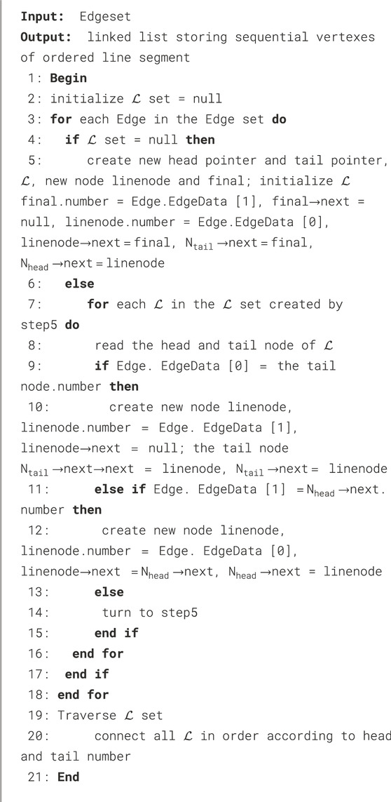
Algorithm 1.Contour line segments sorting.

2.6 The model stitching strategy

To incorporate fine fault models into the original model, we first deleted the conflicting triangular meshes and then stitched the fine fault models into the modified original framework. Combined with the actual problems described in this study and the modeling algorithm used in the previous steps, we introduced an ear clipping algorithm to convert the contour line segments stitching problem into a triangulating problem and construct a surface model for the gap between the two models.

2.6.1 Preprocessing of contour line segments topology structure

Extraction of contour lines:

The outer boundary contour line segments for the fault model and for all the overlapping triangles were extracted using the algorithms described in Section 2.5: ${\widehat{\mathrm{L}}}_{\mathrm{F}}=\mathcal{S}(\mathrm{C}\mathrm{o}\mathrm{n}\mathrm{t}\mathrm{o}\mathrm{u}\mathrm{r}({\mathrm{T}}_{{\mathrm{I}}_{\mathrm{F}}}))$, and ${\widehat{\mathrm{L}}}_{\mathrm{O}}=\mathcal{S}(\mathrm{C}\mathrm{o}\mathrm{n}\mathrm{t}\mathrm{o}\mathrm{u}\mathrm{r}({\mathrm{T}}_{\text{overlap}}))$. Each contour line polygon meets the definition of a simple polygon (assumed as $\mathrm{P}=\left\{\widehat{\mathrm{L}},\mathcal{E}\right\}$), with the following properties:

$•$ $\mathcal{E}=\left\{⟨{\mathit{l}}_{\mathit{i}},{\mathit{l}}_{\mathit{i}+1}⟩\mid 0\le \mathrm{i}\le \mathrm{n}-2\right\}\cup \left\{⟨{\mathit{l}}_{\mathit{n}-1},{\mathit{l}}_0⟩\right\}$; $\forall l_i\in \widehat{\mathrm{L}},\mathrm{deg}(l_i)=2$.

$•$ $\forall {\mathrm{e}}_{\mathrm{i}},{\mathrm{e}}_{\mathrm{j}}\in \mathcal{E}(\mathrm{i}\ne \mathrm{j}),{\mathrm{e}}_{\mathrm{i}}\cap {\mathrm{e}}_{\mathrm{j}}\ne \mathrm{\varnothing }\Rightarrow {\mathrm{e}}_{\mathrm{i}}\cap {\mathrm{e}}_{\mathrm{j}}\subseteq \widehat{\mathrm{L}}$; ${\mathrm{e}}_{\mathrm{i}}\ne {\mathrm{e}}_{\mathrm{j}}\wedge {\mathrm{e}}_{\mathrm{i}}\ne ⟨{\mathrm{e}}_{\mathrm{j}}^1,{\mathrm{e}}_{\mathrm{j}}^0⟩$.

Finding mutually visible vertices:

We preferentially selected the minimum and maximum points on the Y-axis and X-axis of the two polygons. If no mutually visible point is found, this point is taken as the center, and the inner and outer polygons are slid counterclockwise and clockwise for a point distance to determine whether the next point meets the conditions. The shape of the fault model is generally not particularly irregular; therefore, the aforementioned priority points can be determined. If this method fails, it is recommended to use the method of David Eberly to find mutual visible points. The algorithm can be summarized in the Appendix. Finally, a pair of desired visible points is obtained: $({\mathrm{v}}_{\mathrm{a}},{\mathrm{v}}_{\mathrm{b}})$.

2.6.2 Contour lines topological structure reconstruction

Separation of vertex attributes:

Visible points must be copied to different data structures before they can be used. Each data structure stores a current point that may be reflex or convex. Even if two points have the same coordinates, one can be a reflex point and the other can be a convex point.

Bidirectional edge connection:

A simple polygon can be obtained by introducing two coincident edges connecting mutually visible vertices. The outer vertices were ordered counterclockwise, and the inner vertices were ordered clockwise; thus, the topological directions of these two new edges were opposite:

$\mathrm{f}\mathrm{o}\mathrm{r}\left({\mathrm{v}}_{\mathrm{a}},{\mathrm{v}}_{\mathrm{b}}\right),\text{insert\hspace{0.17em}bidirectional\hspace{0.17em}edges\hspace{0.17em}}{\mathrm{e}}_{\mathrm{a}\mathrm{b}}:{\mathrm{v}}_{\mathrm{a}}\to {\mathrm{v}}_{\mathrm{b}}\text{and\hspace{0.17em}}{\mathrm{e}}_{\mathrm{b}\mathrm{a}}:{\mathrm{v}}_{\mathrm{b}}\to {\mathrm{v}}_{\mathrm{a}}.$

Finally, the boundary of the new simple polygon is:

$\mathrm{\partial }{\mathrm{P}}_{\mathrm{N}}=\left({\mathrm{\gamma }}_{\mathrm{k}}\cdot {\widehat{\mathrm{L}}}_{\mathrm{O}}\right)\cup {\mathrm{e}}_{\mathrm{b}\mathrm{a}}\cup {\widehat{\mathrm{L}}}_{\mathrm{F}}\cup {\mathrm{e}}_{\mathrm{a}\mathrm{b}}$

where $\mathrm{\gamma }$ is a direction adjustment factor and $\mathrm{\gamma }\in \left.\left\{+1,-1\right\}\right)$.

When there is a fault without pinching at the boundary of the study area and the fault itself contains boundary information, special treatment is required. We retained the outer boundary of the study area on the fine fault model and used it to replace the outer boundary. The two models at the endpoints of the outer boundary of the study area, together with the internal boundary edges of the two models, formed a polygon without inner holes. The above approach can ensure seamless splicing between the small modules when modeling in sub-regions.

2.6.3 Triangulating the gap between the two models by ear clipping

The ear clipping algorithm (Eberly, 2008) is a triangulation process of constantly looking for ears to remove. Each time an ear is deleted, a polygon with $n\ge 4$ vertices becomes a new polygon with $n-1$ vertices. According to the linked list of the efficient storage and management of data given in David Eberly et al.‘s paper, the algorithm can be briefly summarized as follows: The first step is to initialize the polygons, reflex and convex points, and ear links. For each vertex ${\mathit{l}}_{\mathit{i}}$ on the polygon and corresponding triangle $({\mathit{l}}_{\mathit{i}-1},{\mathit{l}}_{\mathit{i}},{\mathit{l}}_{\mathit{i}+1})$, where $\mathrm{i}$ is the vertex index of the polygons, if there are no points in this triangle other than the three vertices that compose the triangle, the triangle is an ear. The second step is to iterate over the ear links to generate triangles. Each time an ear is deleted, the reflex and convex points, the ear sequence and the vertex sequence are updated. The concavity and convexity of the point adjacent to the ear tip, as well as the ear attributes, may be altered by deleting the ear. We performed an ear test for each update. After the above steps, we can obtain the triangular mesh surface $\mathrm{G}$ of the gaps between the two models. Therefore, the set of triangles on surface G is: ${\mathrm{T}}_{\mathrm{G}}={\mathcal{T}}_{\mathrm{earclipping}}({\mathrm{\pi }}_{\mathrm{x}\mathrm{y}}(\mathrm{\partial }{\mathrm{P}}_{\mathrm{N}}))$, ${\mathcal{T}}_{\mathrm{earclipping}}$ is the ear clipping operator. After providing the elevation for each point, the models were spliced together. The final model was generated as: ${\mathrm{T}}_{\mathrm{final}}={\mathrm{T}}_{\mathrm{S}}\cup {\mathrm{T}}_{{\mathrm{I}}_{\mathrm{F}}}\cup {\mathrm{T}}_{{\mathrm{I}}^{\prime }}\cup {\mathrm{T}}_{\mathrm{G}}$.

3 Data and results

3.1 Overview of test data illustrating

Here, we present a modeling example of this method. The data were the drilling and section data from exploration line I to exploration line supplement6 including exploration line supplement6, a total of nine exploration lines in the study rear. The initial input data for the modeling were the three-dimensional coordinate values extracted from the drilling and section data. The drilling data were numbered hierarchically, and the three-dimensional coordinate set of each layer was extracted. Figure 3 shows the distribution of the boreholes in three dimensions, with a total of 112 boreholes. We took the four-layered stratum elevation values, from top to bottom: the topsoil layer, third impervious bed, eighth coal seam, and tenth coal seam; among them, the eighth coal seam and tenth coal seam are the main mining coal seams. The study area is approximately 4,180 m long from east to west and 4,170 m long from north to south. The topographic surface has been divided into rivers, roads, and other information based on multi-constraint data, with a total of 4,091 data points. And 29,372 point data were used to construct the building complex and railway. The four typical faults in the study area were used for modeling. fault 2F4, which is a general fault; fault F22, which is a boundary fault; and faults 2F1 and 4F2, which form a T-crossing fault. The Cartesian coordinate system was used to present the data model in this study. The four faults include normal faults and reverse faults: faults 2F4 and 2F1 are inverse faults, and F22 and 4F2 are normal. Information on fault lines and pinch-out points was obtained from the plan geological map. The horizontal distribution of the aforementioned faults mentioned above is shown in Figure 4a, and the fault modeling data in this study are all three-dimensional coordinates of the section view. The exploration line profile containing fault F22 is shown in Figure 4b.

Figure 3

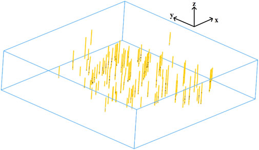
Figure 3. The distribution of borehole in three dimensions of the study area.

Figure 4

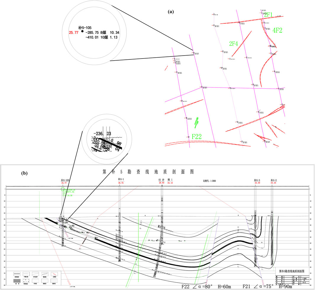
Figure 4. The data for modeling. (a) The horizontal distribution of the faults. (b) The exploration line profile containing fault F22.

3.2 The model details and results

All the algorithms were run on a computer with an NVIDIA GeForce RTX 3060 graphics card. We used .3dt files to store the model and LK LionKing software for visualization. Combined with the data model, data structure, and storage form of the geological body in this study, we used the same object-oriented programming languages, C++ and C$\#$, to implement the algorithms adopted for the modeling.

The initial continuous multi-DEM is shown in Figure 5a, with color coding as follows: topsoil (green), third impervious bed (yellow), eighth coal seam (black), tenth coal seam (dark gray), and simulation layer (brownish yellow). We constructed independent DEM surfaces using Delaunay triangulation for each stratigraphic interface, avoiding a shared TIN template. With the help of mature visualization tools, we divided the two situations to address the intersections between layers: (1) replacing the exposed boreholes with upper-layer elevation data, and (2) inserting the midpoints of the exposed edges into lower-layer datasets for mesh regeneration. A continuous stratigraphic model without intersections can be constructed through iterative adjustments and updates. The details of the two intersection scenarios above are shown in Figure 6: (a) represents an intersection between the eighth and tenth coal seams at the exposed boreholes, with (e) and (f) showing the pre- and post-processing TINs, and (b) depicts the retriangulated mesh after data supplementation. Case (c) demonstrates the intersection at the exposed triangular edges, with (g) and (h) displaying TINs before and after inserting the midpoint coordinates into the tenth seam, as indicated in (d). All algorithms of the modeling strategy for each layer for every fault were performed to obtain a complete multi-DEM containing normal and inverse faults, as shown in Figure 5b.

Figure 5

Figure 5. The 3D geological modeling of research area. (a) The initial geological interfaces, (b) The final geological model.

Figure 6

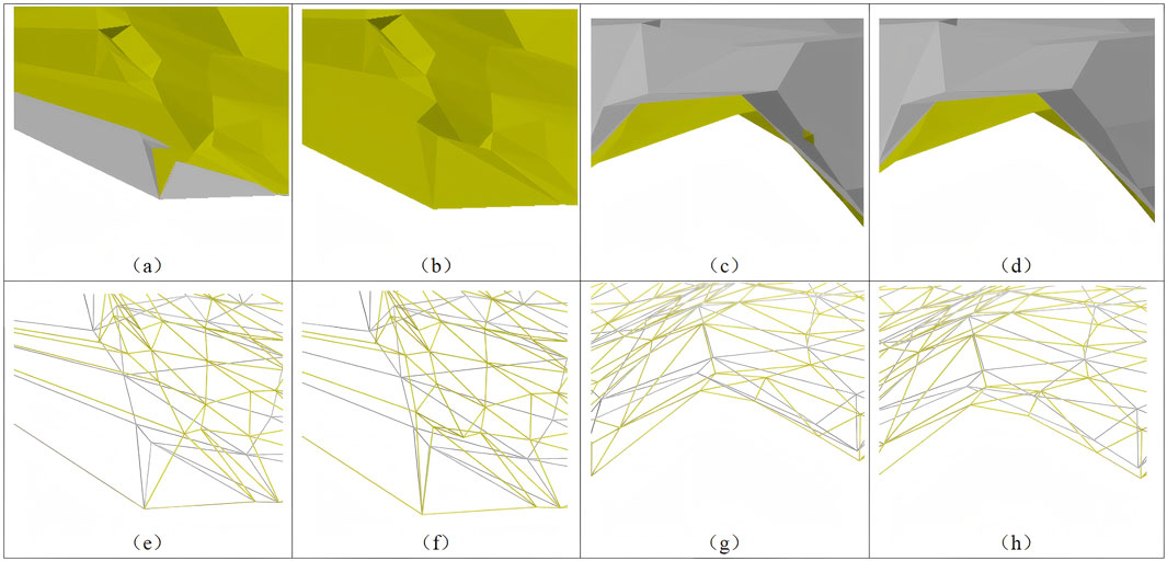
Figure 6. Handling intersection issues. (a, c) are cases dealing with an exposed borehole and exposed triangle edge, respectively. (b, d) are the triangular mesh of retriangulation after supplementing drilling data and entering the midpoint coordinates of the exposed edge. (e, f) are the TIN before and after processing (a), respectively. (g, h) are the TIN before and after processing (c), respectively.

In order to further show the model results, we used vertical planes to cut the geological body to obtain the internal structure and the shape of the geological body on the sections. The cutting plane can be random. Here, we selected the northernmost position of the exploration line complement-6 as the starting point to construct the cut plane, and the azimuth angles of the cutting surface are $317.089497°$, and $18.146639°$ respectively. The cutting process involved multiple intersection operations between the mesh surface and cutting plane, and the results are shown in Figures 7a–c.

Figure 7

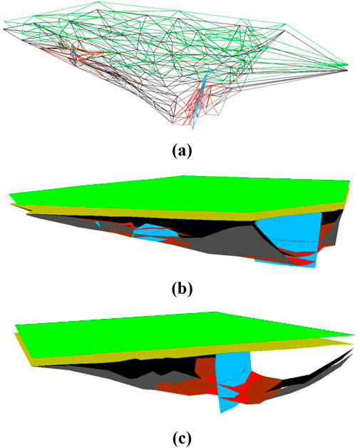
Figure 7. A multi-DEM with four faults (presented from two angles). (a) The triangular mesh surface, (b) $317.089497°$, and (c) $18.146639°$.

Figure 8 shows the splicing results for a stratum layer. The red-brown color is the triangulation of the splicing part between the two models, and the other color parts are the same as above. (a) is the triangular mesh surface embedded fault plans. (b) shows the local details of the triangular mesh surface in the splicing area. (c), (d), and (e) are partially enlarged views of faults F22, 2F4, 2F1 and 4F2, respectively.

Figure 8

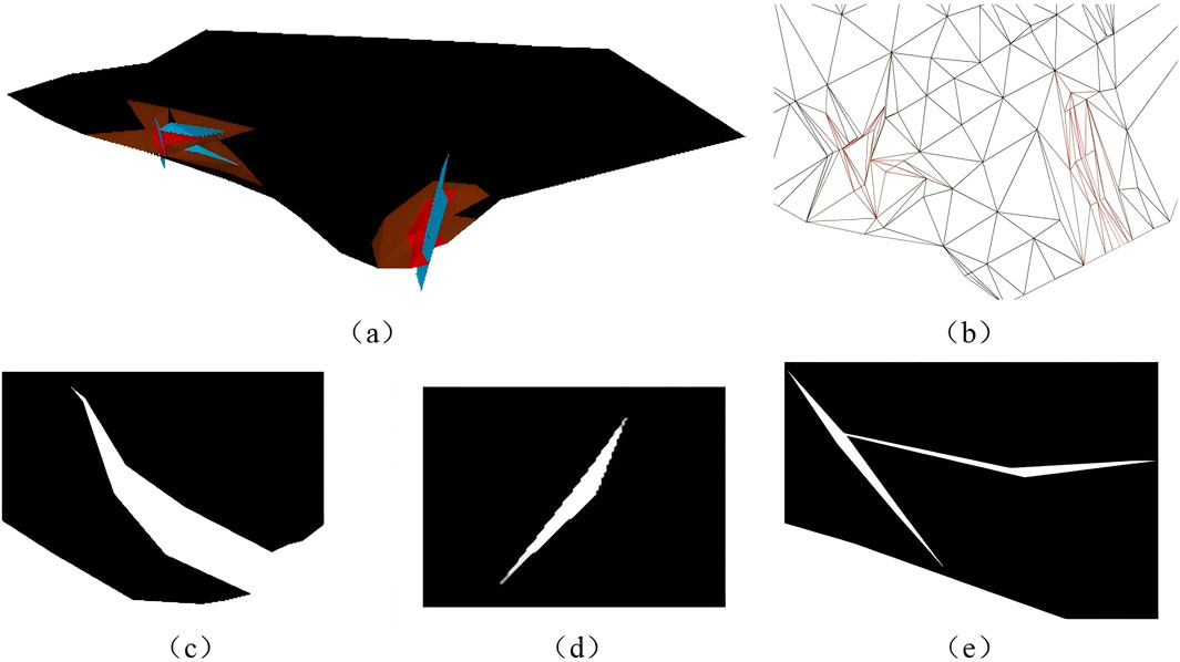
Figure 8. A layer triangular mesh model after stitching a geological horizons and a fault. (a) The triangular mesh surface embedded fault plans; (b) The local details; (c) Fault F22; (d) Fault 2F4; (e) Fault 4F2.

4 Discussion

We consider and provide processing methods for various situations that may arise in modeling, such as ordinary faults, cross-faults, adjacent faults, and faults at the boundaries of the research field. This study addressed these situations in detail and provided engineering modeling examples for many situations. The modeling experiment results in Figures 5–7 show that the modeling method used in this paper is tolerant of various types of faults, and can completes the complex modeling tasks effectively. As shown in Figures 5–7 that our method can smoothly splice models together and entirely satisfy the requirements of geological body modeling. Our reconstruction strategy accommodates the shape of the fragments more strongly and has more effective and practical significance than the general contour reconstruction algorithms for the modeling strategy.

4.1 Compared with similar mesh modeling methods

In the Introduction, a review of the existing literature shows that there are many methods for addressing faults. In this section, the proposed method will be compared with two representative modeling methods, GTP of the mesh-based method (Wu et al., 2020), surface-based cutting method (Song et al., 2019; Sterlacchini and Zanchi, 2003; Chilès et al., 1993; Wu and Xu, 2003; Wu et al., 2015).

4.1.1 Compared with the methods based on cutting (surface-based)

After theoretical research and many practical experiments, many general modeling methods based on fault recovery have been applied to 3D modeling software. SketchUp and ArcGIS were combined to make up for the shortages of ArcGIS for modeling complex geological objects (Song et al., 2019). GoCAD uses multi-source data to generate fine fault planes and buried geological surfaces by projection, constraint, and polyline control (Sterlacchini and Zanchi, 2003). It then obtains the final model of the faults and stratum after the initial stratum surface is cut by the fault network and readjusted by DSI (Chilès et al., 1993). Proper sliding and readjustment along the faults can obtain ideal contact border lines between horizons and faults. The GeoSIS system includes a workflow for the complex modeling of geological bodies, calculating the intersections of faults and coal seams and the intersection displacement, and then moving to form the fault intersections of the hanging wall and footwall (Wu and Xu, 2003; Wu et al., 2015).

Modeling methods based on fault recovery generate an overall stratum model and then calculate and adjust the spatial positions of the intersection lines between the fault and coal seam using Boolean, projection, and intersection operations. Segmentation calculations and mesh reconstruction are the key operations in many fault modeling methods. When the number of intersection points is the same, the number of reconstructed triangles is fixed. Therefore, the modeling data in this study were used to realize the faults processing operation of the recovery methods, which were used as a comparison of our modeling method. We cut the 8th and 10th coal seams by using these four typical faults F22, 2F4, 2F1, and 4F2, and then reconstructed mesh surfaces of these fault planes, the 8th and 10th coal seams. The local details of 8th coal seam and faults are shown in Figure 9.

Figure 9

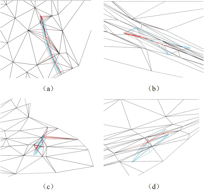
Figure 9. The result of fault cutting 8 coal seam TIN. (a) fault F22 cutting 8 coal seam TIN; (b) fault 4F2 cutting 8 coal seam TIN; (c) fault 2F1 cutting 8 coal seam TIN; and (d) fault 2F4 cutting 8 coal seam TIN.

Table 1 lists the numbers of triangles formed by triangulating the gap between the two models when initial continuous stratum models are spliced with the fault F22 model, fault 2F4 model, and the faults 2F1 and 4F2 models respectively. The initial stratum model used in the modeling method for the data results of 2F4 is the stratum model after stitching the initial continuous stratum model generated in Section 3 and faults 2F1 and 4F2 model or fault 2F1 model. The tenth coal seam did not break or move at the position of fault 4F2 in the study area. The number of the triangles on triangulated gaps and that on the initial models are of the same order of magnitude, which is consistent with the expectations. In addition, Table 1 also lists the number of triangles reconstructed under the constraints of the intersection point and line using the comparison method. This number is the total number of triangles that include intersection points and have been reconstructed on both fault mesh surfaces and stratigraphic mesh surfaces. Reducing the number of narrow and elongated triangles in mesh modeling can enhance numerical stability and simulation accuracy, improve convergence speed, lower computational costs, and increase overall mesh quality. We calculateed the degrees of interior angles of the triangles in the mesh model and classified any triangle with an interior angle below 20° or 10° as a narrow or elongated triangles. Table 2 lists the ratios of narrow and elongated triangles to newly generated triangles from the experimental results of the two different methods. Table 2 shows that, except for 2F4 on the 8th coal seam, all the ratios obtained by our method were smaller than those obtained by the methods based on cutting. From Figures 8, 9 and Table 1, 2, it is known that the modeling method based on mesh segmentation generates much more triangles than the method in this paper, which leads to more long and narrow triangles. The finer the fault plane and stratum grid, the more intersection points there are; thus, the number of reconstructed triangles increases rapidly. In our modeling framework, collision detection and mesh reconstruction based on two-dimensional topological relationships are implemented faster. Moreover, the fine fault model and continuous strata are not cut; therefore, the fault planes and the number of reconstructed triangles are not affected by the intersection points. A large number of long and narrow triangles are undesirable in modeling. In addition, the intersecting operation between the faults plane and the stratum surfaces is tolerant of normal faults, but the fault lines on the hanging wall and footwall of the reverse fault cannot be described well. The sliding and readjustment of intersection points and our method can finely describe the fault intersections of the hanging wall and footwall of the normal and reverse faults. However, ensuring the accuracy of the direction and distance of displacement is labor intensive. Therefore our method is simpler and labor-saving. In general, the efficiency, accuracy and automation of our method are higher, and it is more obvious when there are many faults that needed to be processed.

Table 1

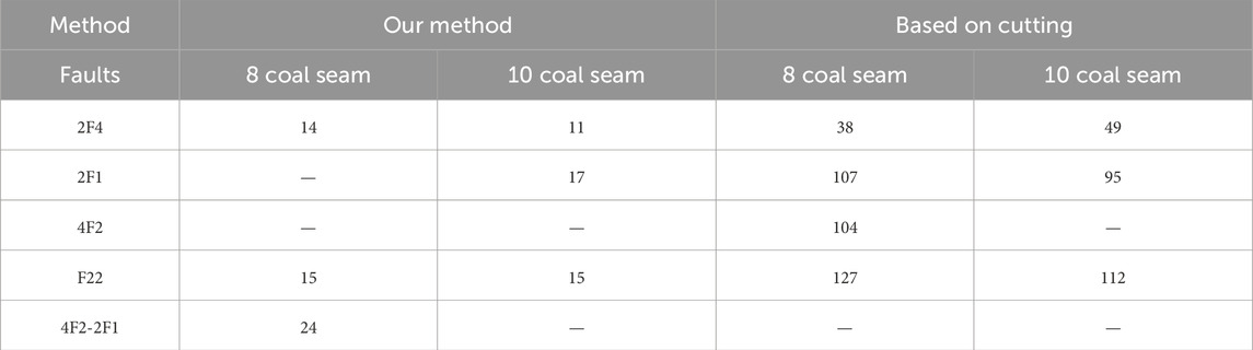
Table 1. The number of triangles after retriangulation.

Table 2

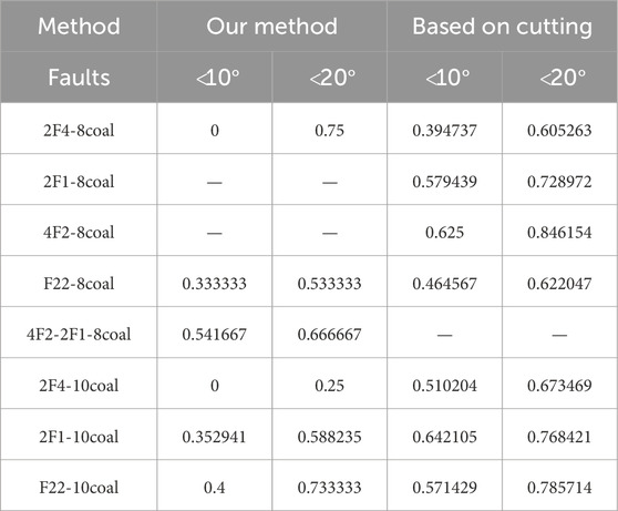
Table 2. The proportion of narrow triangles.

4.1.2 Compared with the methods based on GTP (volume-based)

In the modeling method based on volume model, three-dimensional models based on triangular prisms perform well in modeling complex geological bodies. Using GTP as the basic solid element model, (Guo et al., 2011) used parameters as a degradation mechanism to generate a geological entity model with strata pinch. The authors of Liu et al. (2012)) integrated a similar tri-prism model and a traditional multi-layer TIN model. A 3D geosciences modeling system, GeoMo3D, was developed based on GTP, which can successfully process strata bifurcation, thinning, pinch out and faults (Wu et al., 2020).

The terrain surface TIN serves as the foundation for constructing GTP. There are typically two approaches for processing fault plane combinations based on GTP: one is similar to the geological interface cutting method described in the previous section, which involves cutting the GTP body using fault planes. The other approach involves the geological structure knowledge-reasoning rules among boreholes established by Chen Xuexi et al., which enable the automatic modeling of GTP based on borehole numbers and geological rules. The previous section compared methods similar to the first one mentioned above. This section discusses the comparison between the method used in this paper and the second approach for GTP. When generating a GTP model containing faults, this method faces several challenges compared to the method proposed in this paper: (1) A few boreholes simultaneously cross a fault plane. To represent the complete geometric morphology of the fault, it is necessary to add multiple virtual boreholes. (2) According to the modeling rules of GTP, the number of boreholes in each coal seam is the same. To represent the morphology of the fault surface, a TIN constrained by the intersection lines of faulted coal seams must be generated in the top layer. The numerous faults or discontinuous layers will result in numerous constraints. 3: Additionally, if refinement of object morphologies such as buildings, rivers, plains, and mountains on the surface is required, a TIN constrained by the object morphologies needs to be generated. Figures 10a, b respectively show magnified views of the architectural details and the topological structure and locations of rivers, terrain and a large borehole within the overall model. As shown in Figure 10a, the corresponding river and mining enterprise information in the modeling area of this paper is generated. In this case, a single borehole may not be able to simulate the surface information; therefore, we prefer methods that allow for different mesh topologies for each layer. Figure 10a illustrates the comparison between the constrained points on the mesh surface and the actual large underground borehole locations in the case study used in this paper. 4: Experiments by Lyu et al. have shown that data conflicts arise when using the borehole data provided in their paper for TIN mesh modeling in multi-valued regions. Therefore, modeling based on GTP for reverse faults or more complex faults may result in errors. Consequently, the method proposed in this paper and other modeling methods based on the surface and B-rep concepts are more flexible and concise in terms of the data points at various layers and morphological descriptions. Moreover, the method proposed in this paper is more reliable than GTP based on knowledge-reasoning rules when dealing with ancient faults.

Figure 10

Figure 10. The overall model. (a) The topology and location of the rivers, topography and large borehole; (b) the architectures model.

4.2 Qualitative comparison with mesh and non-mesh modeling methods

A comparative analysis of the mathematical modeling from the key references in the Introduction is summarized in Table 3. The parametric NURBS method achieves geological model construction and updating with NURBS Surface Dynamic Topology (NURBS-SDT) and Boolean Logic Sequence of Oriented Geological Interfaces (BLSOGI). NURBS-SDT enables highly automated surface construction and excels in modeling folds and intrusions. However, the rules of BLSOGI are defined based on expert knowledge, and the substructure becomes relatively complex when when multiple faults are involved. The GTP based on the expansion algorithm is highly automated and capable of describing internal attribute fields. However, Lyu et al. demonstrated that in multivalued regions (e.g., boreholes with multiple demarcation points), conflicting data during TIN generation reduces its effectiveness for complex and reverse faults. Early studies based on machine learning for stratigraphic modeling focused on the architecture of deep learning, lacked comparative analyses and addressed the issue of discontinuities caused by faults. Recent work has shown that deep learning-based geological modeling methods enables high-precision and flexible multi-source data integration, despite requiring labeling data for effective model training. However, we must assess whether the high cost of labeled data generation in geological engineering is justified, and whether enough quality data can be obtained. In this study, the geological interface still is TIN. Although TIN lacks the smoothness and multi-source data integration capabilities comparing with like neural networks and RBFs, it is the preferred format for visualization for various methods (e.g., scattered point interpolation, function surface modeling). However, discontinuous regions caused by faults require additional processing. The current constraint line and cutting-based methods only embed fault line boundaries into grids (as shown in Figure 9). These improved methods require moving breakpoints and separately interpolating hanging and footwall meshes to better represent faults and adjacent structures. This complexity stems from the need for task-specific expertise and meticulous adjustments to interpolation algorithms, parameters and scope. A favorable aspect is that TIN is compatible with various high-precision modeling techniques (e.g., RBF implicit methods and potential field methods) for grid interpolation, thereby generating higher-accuracy surfaces. Therefore, our method outperforms fault-handling methods in flexibility, automation, robustness, and mesh quality.

Table 3

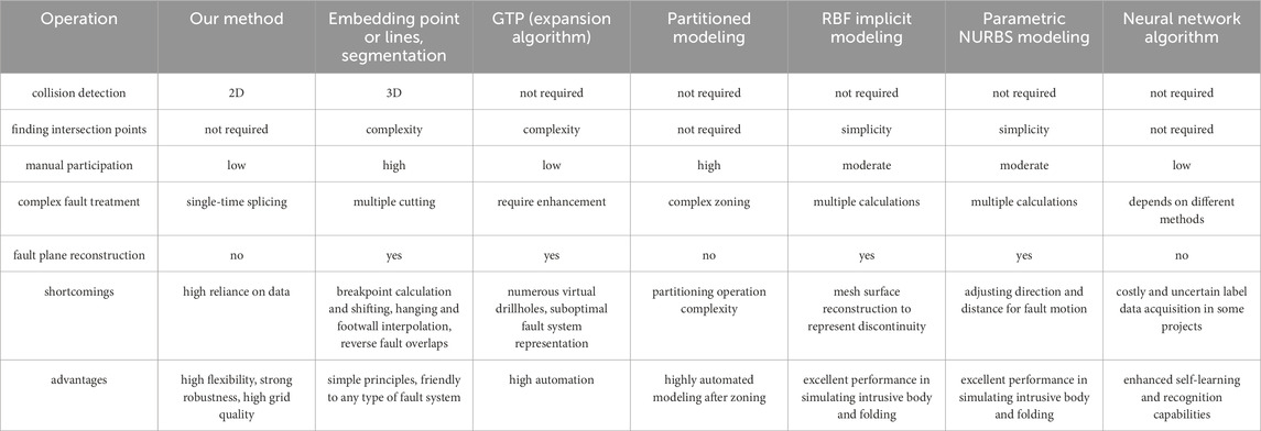
Table 3. The comparative analysis of various methods for handling faults.

4.3 Limitations and future work

The modeling method described in this paper does, however, have some limitations and shortcomings: (1) Single deterministic models representing unknown underground geological structures cannot reflect inherent geological uncertainties. Uncertainty or error may be introduced in the measurement of the original data, the drawing of geological maps based on the analysis of the original data and the inferred geological structure, and the modeling method using geological map data. Therefore, it is important to use multiple model realizations to quantify uncertainty. Geological modeling methods based on geostatistics can quantify these geology uncertainties (Yin et al., 2020), and computer stochastic simulation methods enable the assessment of uncertainty in the forecasts (Satija et al., 2017). (2) Insufficient data or data conflicts when generating the fault models, which is normal in modeling. For extremely complex fault intersection networks, the derivation of the fault model data is recommended. Among them, we can decompose stepped faults, grabens, horsts, and en echelon faults into individual normal and reverse faults or cross faults based on actual conditions. In contrast, circular faults and radial faults are relatively rare and formed in special environments that are often associated with volcanic activity or localized stress concentrations. This paper suggests that by slicing the 3D seismic data cube into multi-sectional views and performing precise fault exploration, more data can be obtained to describe such complicated faults.

In addition, it is necessary to check the fine fault models to ensure that there is no overlap between the fault models before retriangulating of the gap of two models. However, the completion of geological modeling can be guaranteed, and fault models are generated multiple times in the worst-case scenario. We believe that the modeling method in this paper not only is suitable for fault modeling but also can be used to replace the initial coarse-precision model part with any accurate data partial model based on surfaces. For example, multi-valued folds and a detailed description of anticlines and synclines can be embedded in the initial model using the replacing-and-stitching method proposed in this study. Only the fault model in this study would need to be replaced with other models. The process and intermediate processing method would be the same, so the modeling strategy demonstrates broad applicability.

Therefore, our method has the potential for further research. In the future, we hope to determine the optimal visible point when reconstructing the irregular triangulated surfaces between the contour lines of the two models used in this study, ensuring that the geological body model is smoother and more harmonious. We believe that the order of the ear sequence is also a breakthrough point in optimizing the triangle. More efforts should be made to improve the accuracy and fineness of the model with limited data and provide a simple operation interface for actual engineering needs. In addition, when obtaining a more reliable stratum surface within the range of influence of the fault, a more detailed fault plane should be established without crossover, while a seamless integration between the fault plane and the geological body should be ensured.

More interpretation outputs within statistically robust confidence thresholds can be obtained by applying high-precision exploration technologies and automated interpretation algorithms, particularly neural networks, for geological data analysis. We believe that coupled modeling integrating the interpretation outputs and sparse drilling data points could provide more constraints and descriptive information for geological models.

Furthermore, future investigations could explore the feasibility of direct integration between sparse borehole datasets and raw exploration data (e.g., unprocessed seismic volumes), thereby not only enhancing multi-source constraint propagation but also circumventing structural biases introduced by intermediately processed 3D volumetric models. This paradigm shift would prioritize first-principles data fusion over conventional sequential processing workflows.

5 Conclusion

The modeling of complex geological bodies is an important research topic. To address the problem of geometric modeling, this paper proposes a flexible modeling method for geological bodies containing normal and inverse faults. This paper proposes a reconstruction strategy using the ear clipping method, which is compatible and transitional with the stratigraphic planes constructed by using the two-dimensional triangulation algorithm used in our modeling method, and makes the triangulation network of the strata more realistic. Additionlly, this paper proposes a contour sorting algorithm that is flexible, simple, highly portable, and indispensable for the modeling process used in this study and other engineering applications. The modeling experiment results show that the accurate model fragments and stratum surfaces constructed by a two-dimensional triangulated irregular network generation algorithm are perfectly combined. By constantly performing substitution and reconstruction operations, multi-layer triangular mesh models of complex geological bodies can be generated. The fault lines, the hanging wall and footwall surfaces within the range of influence of the fault are automatically and accurately described. The precision of the normal and inverse fault models is improved and the difficulty of overall modeling is reduced. Furthermore, this method reduces manual interaction, improves the efficiency of modeling complex geological bodies and the quality of the triangular mesh. So it is a method with academic research and engineering practice value. This research contributes to improving the mining efficiency, reducing safety risks, and promoting the intelligent development of mines.

Data availability statement

The data analyzed in this study is subject to the following licenses/restrictions: The dataset is private and can only be obtained through specific channels or with authorization. Secondary analysis of the data or the development of new research products from it is prohibited unless written consent is obtained from the data provider. Requests to access these datasets should be directed to Z2Fvd2w5MUAxNjMuY29t.

Author contributions

WG: Methodology, Writing – original draft, Writing – review and editing. XL: Funding acquisition, Project administration, Supervision, Writing – review and editing. SH: Formal Analysis, Writing – review and editing. TZ: Data curation, Writing – review and editing, Formal Analysis. WL: Data curation, Writing – review and editing.

Funding

The author(s) declare that financial support was received for the research and/or publication of this article. Central Guidance Fund for Local Scientific and Technological Development (YDZX2022097) Grant Recipient: Xinming Lu.

Acknowledgments

The authors appreciate the Shandong Languang Software Co., Ltd. for providing the exploration data and Smart Mine Platform.

Conflict of interest

The authors declare that the research was conducted in the absence of any commercial or financial relationships that could be construed as a potential conflict of interest.

Generative AI statement

The author(s) declare that no Generative AI was used in the creation of this manuscript.

Publisher’s note

All claims expressed in this article are solely those of the authors and do not necessarily represent those of their affiliated organizations, or those of the publisher, the editors and the reviewers. Any product that may be evaluated in this article, or claim that may be made by its manufacturer, is not guaranteed or endorsed by the publisher.

References

Biniaz, A., and Dastghaibyfard, G. (2012). A faster circle-sweep delaunay triangulation algorithm. Adv. Eng. Softw. 43, 1–13. doi:10.1016/j.advengsoft.2011.09.003

CrossRef Full Text | Google Scholar

Chai, C., and Maceira, M. (2022). Machine learning enhanced seismic monitoring at 100 km and 10 m scales. Oak Ridge, TN (United States): Oak Ridge National Laboratory ORNL.

Google Scholar

Che, D., and Jia, Q. (2019). Three-dimensional geological modeling of coal seams using weighted kriging method and multi-source data. Ieee Access 7, 118037–118045. doi:10.1109/access.2019.2936811

CrossRef Full Text | Google Scholar

Chilès, J.-P., Courrioux, G., Deverly, F., and Renard, P. (1993). 3-d geometric modelling of fault and layer systems using gocad software: example of the soultz horst (alsace, France). Geoinformatics 4, 209–218. doi:10.6010/geoinformatics1990.4.3_209

CrossRef Full Text | Google Scholar

Dianzhu, S., Xincheng, L., Zhongchao, T., and Yanrui, L. (2009). Accelerated boolean operations on triangular mesh models based on dynamic spatial indexing. Journalof Comput. and Computergr. 21, 1232G1237. doi:10.1115/MNHMT2009-18287

CrossRef Full Text | Google Scholar

Eberly, D. (2008). Triangulation by ear clipping. Geometric. Tools., 2002–2005.

Google Scholar

Frank, T., Tertois, A.-L., and Mallet, J.-L. (2007). 3d-reconstruction of complex geological interfaces from irregularly distributed and noisy point data. Comput. and Geosciences 33, 932–943. doi:10.1016/j.cageo.2006.11.014

CrossRef Full Text | Google Scholar

Fuchs, H., Kedem, Z. M., and Uselton, S. P. (1977). Optimal surface reconstruction from planar contours. Commun. ACM 20, 693–702. doi:10.1145/359842.359846

CrossRef Full Text | Google Scholar

Guo, J., Li, Y., Jessell, M. W., Giraud, J., Li, C., Wu, L., et al. (2021). 3d geological structure inversion from noddy-generated magnetic data using deep learning methods. Comput. and Geosciences 149, 104701. doi:10.1016/j.cageo.2021.104701

CrossRef Full Text | Google Scholar

Guo, J., Wu, L., Zhou, W., Jiang, J., and Li, C. (2016). Towards automatic and topologically consistent 3d regional geological modeling from boundaries and attitudes. ISPRS Int. J. Geo-Information 5, 17. doi:10.3390/ijgi5020017

CrossRef Full Text | Google Scholar

Guo, J., Wu, L., Zhou, W., Li, C., and Li, F. (2018). Section-constrained local geological interface dynamic updating method based on the hrbf surface. J. Struct. Geol. 107, 64–72. doi:10.1016/j.jsg.2017.11.017

CrossRef Full Text | Google Scholar

Guo, J., Yang, Y., Wu, L., and Zhang, R. (2011). “A novel method for modeling complex 3d geological body with stratal pinch-out,” in 2011 IEEE international Geoscience and remote sensing symposium (IEEE), 4204–4207.

Google Scholar

He, Z., Wu, C., Tian, Y., and Mao, X. (2008). Three-dimensional reconstruction of geological solids based on section topology reasoning. Geo-spatial Inf. Sci. 11, 201–208. doi:10.1007/s11806-008-0082-2

CrossRef Full Text | Google Scholar

Hillier, M. J., Schetselaar, E. M., De Kemp, E. A., and Perron, G. (2014). Three-dimensional modelling of geological surfaces using generalized interpolation with radial basis functions. Math. Geosci. 46, 931–953. doi:10.1007/s11004-014-9540-3

CrossRef Full Text | Google Scholar

Hua, W.-H., Deng, W.-P., Liu, X.-G., and Shang, J.-G. (2006). Improved partition algorithm between triangulated irregular network. Earth Sci. 31, 619–623. doi:10.1360/jos172601

CrossRef Full Text | Google Scholar

Jessell, M. (2001). Three-dimensional geological modelling of potential-field data. Comput. and Geosciences 27, 455–465. doi:10.1016/s0098-3004(00)00142-4

CrossRef Full Text | Google Scholar

Jia, Q., Che, D., and Li, W. (2019). Effective coal seam surface modeling with an improved anisotropy-based, multiscale interpolation method. Comput. and Geosciences 124, 72–84. doi:10.1016/j.cageo.2018.12.008

CrossRef Full Text | Google Scholar

Jia, Q., Li, W., and Che, D. (2020). A triangulated irregular network constrained ordinary kriging method for three-dimensional modeling of faulted geological surfaces. IEEE Access 8, 85179–85189. doi:10.1109/access.2020.2993050

CrossRef Full Text | Google Scholar

Jun-Qi, L., Xiao-Ping, M., Chong-Long, W., and Zhang, Q. (2013). Study on a computing technique suitable for true 3d modeling of complex geologic bodies. J. Geol. Soc. India 82, 570–574. doi:10.1007/s12594-013-0189-1

CrossRef Full Text | Google Scholar

Kaufmann, O., and Martin, T. (2009). Reprint of 3d geological modelling from boreholes, cross-sections and geological maps, application over former natural gas storages in coal mines[comput. geosci. 34 (2008) 278–290]. Comput. and geosciences 35, 70–82. doi:10.1016/s0098-3004(08)00227-6

CrossRef Full Text | Google Scholar

Keppel, E. (1975). Approximating complex surfaces by triangulation of contour lines. IBM J. Res. Dev. 19, 2–11. doi:10.1147/rd.191.0002

CrossRef Full Text | Google Scholar

Lemon, A. M., and Jones, N. L. (2003). Building solid models from boreholes and user-defined cross-sections. Comput. and geosciences 29, 547–555. doi:10.1016/s0098-3004(03)00051-7

CrossRef Full Text | Google Scholar

Lin, L., Li, C., Wei, H., Zhong, Z., Wang, X., Li, Q., et al. (2025). An improved parametric 3d geological modeling framework for seismic structure identification using deep learning in complex geological settings. Geophysics 90, 1–93. doi:10.1190/geo2024-0532.1

CrossRef Full Text | Google Scholar

Liu, G., Hu, Y.-l., and Deng, L. (2003). Discussion on the algorithm of reconstructing the superposition 3-d surface. JOURNAL-CHENGDU Univ. Technol. 30, 537–540. doi:10.1007/s11769-003-0044-1

CrossRef Full Text | Google Scholar

Liu, L., Li, T., and Ma, C. (2024). Research on 3d geological modeling method based on deep neural networks for drilling data. Appl. Sci. 14, 423. doi:10.3390/app14010423

CrossRef Full Text | Google Scholar

Liu, S. H., Wang, X. H., and Jun, T. (2012). Study on the method of 3d geologic modeling and visualization. Appl. Mech. Mater. 220, 2862–2865. doi:10.4028/www.scientific.net/amm.220-223.2862

CrossRef Full Text | Google Scholar

Lo, S., and Wang, W. (2004). A fast robust algorithm for the intersection of triangulated surfaces. Eng. Comput. 20, 11–21. doi:10.1007/s00366-004-0277-3

CrossRef Full Text | Google Scholar

Lyu, M., Ren, B., Wu, B., Tong, D., Ge, S., and Han, S. (2021). A parametric 3d geological modeling method considering stratigraphic interface topology optimization and coding expert knowledge. Eng. Geol. 293, 106300. doi:10.1016/j.enggeo.2021.106300

CrossRef Full Text | Google Scholar

Mei, G., Tipper, J. C., and Xu, N. (2012). “Ear-clipping based algorithms of generating high-quality polygon triangulation,” in Proceedings of the 2012 international conference on information technology and software engineering: software engineering and digital media technology (Springer), 979–988.

Google Scholar

Ming, J., Pan, M., Qu, H., and Ge, Z. (2010). Gsis: a 3d geological multi-body modeling system from netty cross-sections with topology. Comput. and Geosciences 36, 756–767. doi:10.1016/j.cageo.2009.11.003

CrossRef Full Text | Google Scholar

Qu, H., Pan, M., Wang, Z., Wang, B., Chai, H., and Xue, S. (2006). A new method for 3d geological reconstruction from intersected cross-sections. Remote Sens. Space Technol. Multidiscip. Res. Appl. (SPIE) 6199, 202–210.

Google Scholar

Rebay, S. (1993). Efficient unstructured mesh generation by means of delaunay triangulation and bowyer-watson algorithm. J. Comput. Phys. 106, 125–138. doi:10.1006/jcph.1993.1097

CrossRef Full Text | Google Scholar

Renard, P., and Courrioux, G. (1994). Three-dimensional geometric modeling of a faulted domain: the soultz horst example (alsace, France). Comput. and Geosciences 20, 1379–1390. doi:10.1016/0098-3004(94)90061-2

CrossRef Full Text | Google Scholar

Satija, A., Scheidt, C., Li, L., and Caers, J. (2017). Direct forecasting of reservoir performance using production data without history matching. Comput. Geosci. 21, 315–333. doi:10.1007/s10596-017-9614-7

CrossRef Full Text | Google Scholar

Song, R., Qin, X., Tao, Y., Wang, X., Yin, B., Wang, Y., et al. (2019). A semi-automatic method for 3d modeling and visualizing complex geological bodies. Bull. Eng. Geol. Environ. 78, 1371–1383. doi:10.1007/s10064-018-1244-3

CrossRef Full Text | Google Scholar

Sterlacchini, S., and Zanchi, A. (2003). “3d reconstruction of subsurface geological bodies: methods and applications,” in The annual conference of the international association for mathematical geology, 756–764.

Google Scholar

Tertois, A.-L., and Mallet, J.-L. (2007). “Editing faults within tetrahedral volume models in real time,”, 292. Geological Society, London, Special Publications, 89–101. doi:10.1144/sp292.5

CrossRef Full Text | Google Scholar

Tipper, J. C. (1976). The study of geological objects in three dimensions by the computerized reconstruction of serial sections. J. Geol. 84, 476–484. doi:10.1086/628213

CrossRef Full Text | Google Scholar

Trubetskoy, K., Galchenko, Y. P., and Sabyanin, G. (2012). Evaluation methodology for structural complexity of ore deposits as development targets. J. Min. Sci. 48, 1006–1015. doi:10.1134/s1062739148060081

CrossRef Full Text | Google Scholar

Tucker, G. E., Lancaster, S. T., Gasparini, N. M., Bras, R. L., and Rybarczyk, S. M. (2001). An object-oriented framework for distributed hydrologic and geomorphic modeling using triangulated irregular networks. Comput. and Geosciences 27, 959–973. doi:10.1016/s0098-3004(00)00134-5

CrossRef Full Text | Google Scholar

Walker, R. J., and Snoeyink, J. (1999). “Practical point-in-polygon tests using csg representations of polygons,” in Workshop on algorithm engineering and experimentation (Springer), 114–128.

Google Scholar

Wu, L. (2004). Topological relations embodied in a generalized tri-prism (gtp) model for a 3d geoscience modeling system. Comput. and Geosciences 30, 405–418. doi:10.1016/j.cageo.2003.06.005

CrossRef Full Text | Google Scholar

Wu, M., Li, H., and Mao, Y. (2020). An automatic three-dimensional geological engineering modeling method based on tri-prism. Arabian J. Geosciences 13, 358. doi:10.1007/s12517-020-05406-7

CrossRef Full Text | Google Scholar

Wu, Q., and Xu, H. (2003). An approach to computer modeling and visualization of geological faults in 3d. Comput. and Geosciences 29, 503–509. doi:10.1016/s0098-3004(03)00018-9

CrossRef Full Text | Google Scholar

Wu, Q., and Xu, H. (2014). Three-dimensional geological modeling and its application in digital mine. Sci. China Earth Sci. 57, 491–502. doi:10.1007/s11430-013-4671-9

CrossRef Full Text | Google Scholar

Wu, Q., Xu, H., and Zou, X. (2005). An effective method for 3d geological modeling with multi-source data integration. Comput. and geosciences 31, 35–43. doi:10.1016/j.cageo.2004.09.005

CrossRef Full Text | Google Scholar

Wu, Q., Xu, H., Zou, X., and Lei, H. (2015). A 3d modeling approach to complex faults with multi-source data. Comput. and Geosciences 77, 126–137. doi:10.1016/j.cageo.2014.10.008

CrossRef Full Text | Google Scholar

Xiang-bin, M., Zhi-qiang, W., Long-Bin, S., and Jian, C. (2010). “Achieving complex geological object solid modeling based on tin and ten,” in 2010 third international conference on information and computing (IEEE), 4, 320–324. doi:10.1109/icic.2010.352

CrossRef Full Text | Google Scholar

Yang, Z., Chen, Q., Cui, Z., Liu, G., Dong, S., and Tian, Y. (2022). Automatic reconstruction method of 3d geological models based on deep convolutional generative adversarial networks. Comput. Geosci. 26, 1135–1150. doi:10.1007/s10596-022-10152-8

CrossRef Full Text | Google Scholar

Yin, Z., Strebelle, S., and Caers, J. (2020). Automated Monte Carlo-based quantification and updating of geological uncertainty with borehole data (autobel v1. 0). Geosci. Model Dev. 13, 651–672. doi:10.5194/gmd-13-651-2020

CrossRef Full Text | Google Scholar

Zhang, B.-y., Wu, X.-b., Wang, L.-f., Liu, X.-g., and Wu, X.-c. (2010). The preliminary research of feature-based 3d geological modeling. 2010 2nd Conf. Environ. Sci. Inf. Appl. Technol. (IEEE) 2, 321–325. doi:10.1109/esiat.2010.5567357

CrossRef Full Text | Google Scholar

Zhang, Y., Zhong, D., Wu, B., Guan, T., Yue, P., and Wu, H. (2018a). 3d parametric modeling of complex geological structures for geotechnical engineering of dam foundation based on t-splines. Computer-Aided Civ. Infrastructure Eng. 33, 545–570. doi:10.1111/mice.12343

CrossRef Full Text | Google Scholar

Zhang, Z., Yin, Z., and Yan, X. (2018b). A workflow for building surface-based reservoir models using nurbs curves, coons patches, unstructured tetrahedral meshes and open-source libraries. Comput. and geosciences 121, 12–22. doi:10.1016/j.cageo.2018.09.001

CrossRef Full Text | Google Scholar

Zhong, D., Li, M., and Liu, J. (2007). 3d integrated modeling approach to geo-engineering objects of hydraulic and hydroelectric projects. Sci. China Ser. E Technol. Sci. 50, 329–342. doi:10.1007/s11431-007-0042-0

CrossRef Full Text | Google Scholar

Zhong, D.-Y., Wang, L.-G., Jia, M.-T., Bi, L., and Zhang, J. (2019a). Orebody modeling from non-parallel cross sections with geometry constraints. Minerals 9, 229. doi:10.3390/min9040229

CrossRef Full Text | Google Scholar

Zhong, D. Y., Wang, L. G., Lin, B. I., and Jia, M. T. (2019b). Implicit modeling of complex orebody with constraints of geological rules. Trans. Nonferrous Metals Soc. China 29, 2392–2399. doi:10.1016/s1003-6326(19)65145-9

CrossRef Full Text | Google Scholar

Zhong, D.-Y., Wang, L.-G., and Wang, J.-M. (2021). Combination constraints of multiple fields for implicit modeling of ore bodies. Appl. Sci. 11, 1321. doi:10.3390/app11031321

CrossRef Full Text | Google Scholar

Zhu, L.-f., Zheng, H., Xin, P., and Wu, X.-c. (2006). An approach to computer modeling of geological faults in 3d and an application. J. China Univ. Min. Technol. 16, 461–465. doi:10.1016/s1006-1266(07)60048-0

CrossRef Full Text | Google Scholar

Appendix

The algorithm for finding mutually visible points

David Eberly et al. provided a method for finding mutually visible points.

1. Find a point on the inner polygon with the maximum x-value. This point is set as the reference point $M$.

2. Let $M$ be the origin of the ray $M+t(\mathrm{1,0})$. The ray will intersect edges $(v_i,v_{i+1})$ of the outer polygon on $I$. Let $I$ be the closest visible point to $M$ on this ray.

3. If $I$ is a vertex of the outer polygon, then $M$ and $I$ are mutually visible and the algorithm terminates.

4. Otherwise, $I$ is on the edge $(v_i,v_{i+1})$. Let $P$ be the endpoint of the maximum x-value for this edge.

5. For triangle $MIP$, if there is no point that is strictly inside the triangle $MIP$, then $M$ and $P$ are mutually visible and the algorithm terminates.

6. Otherwise, at least one reflex vertex is inside the triangle $MIP$; choose the reflex $R$ that minimizes the angle between the line segment $MR$ and ray $M+t(\mathrm{1,0})$. Then, $M$ and $R$ are mutually visible and the algorithm terminates. If there are multiple reflex vertexes that that meet the above conditions, choose the reflex vertex that is the closest to $M$.

Bowyer-Watson algorithm

The main steps of the Bowyer-Watson algorithm are summarized as follows:

1. Generate the simple initial Delaunay triangulated network by constructing two adjacent triangles formed by a quadrilateral enclosing all the scattered points, and put the triangles into the triangle linked list.

2. Insert the scattered points into the point set one by one, and find the triangle whose circumcircle contains the insertion point in the triangle list. This triangle are called the influence triangle of the point. Delete the common edge of the influence triangle and connect the insertion point to all the vertices of the influence triangles to form new triangles. Put the newly formed triangles into the Delaunay triangle list to complete the insertion of a point.

3. Repeat Step 2 above until all the scattered points are inserted.

4. Delete all triangles containing the vertices of the initial triangles in step1.