A riverbank erosion early warning system (EWS-RE) for braided river: a case of the Brahmaputra–Jamuna

Braided rivers are distinguished by numerous bars and channels, along with their regular alterations. This unique character of braided rivers induces bank adjustment through erosion or accretion, and when erosion occurs in populated regions, it results in significant disasters. When such erosion affects inhabited areas, it can cause severe damage. To address this calamity, we introduce here an early warning system for riverbank erosion, named EWS-RE. This system issues alerts based on numerical simulations from a two-dimensional hydro-morphological model of the Brahmaputra–Jamuna River. The forecast model incorporates GloFAS seasonal forecasts and over six decades of historical hydraulic data to define boundary conditions. High-resolution bathymetry of the braided river was generated using an enhanced passive bathymetry technique, which combines satellite imagery with limited in-situ cross-sectional measurements. Model outputs and predicted erosion patterns were validated against actual riverbank changes observed in the year 2019. The system achieved a spatial erosion prediction accuracy of 88% and a sensitivity of 88%, both within a 95% confidence interval. Field testing in the year 2023 showed an overall accuracy of 70% in detecting erosion-prone areas along the river. We anticipate that this framework will contribute significantly to reducing the adverse impacts of riverbank erosion through timely and reliable early warnings.

1 Introduction

Numerous bars and channels, along with frequent changes in bedforms, confluences, and bifurcations, are the well-known traits of braided rivers (Lane, 1957). One of the major management concerns for such rivers is tracking their transformation and managing them appropriately because they change their geometry and planform so rapidly, leading to riverbank adjustment through erosion or accretion (Balouchi et al., 2024; Best et al., 2007; Piégay et al., 2006). Globally, regardless of the river type, riverbank erosion (for rivers exceeding 150 m in width) exhibits an almost log-normal distribution, with a median value of 1.52 m/yr, and poses a serious risk to the people and infrastructure (Langhorst et al., 2022). For example, in Bangladesh [Ganges–Brahmaputra–Meghna (GBM) delta], an average of 60,000 people are displaced due to riverbank erosion (Islam and Mitra, 2024; Kaiser, 2023; Mutton and Haque, 2004). The riverbank erosion rate in the GBM delta is higher than the global average, and the major contributor is the erosion in the braided rivers of the deltas (CEGIS, 2023; Langhorst et al., 2022). For example, the Brahmaputra–Jamuna erosion rate has been alarmingly high for the last four decades, at 17.05 square kilometers per year (Bryant and Mosselman, 2017). However, to the best of our knowledge, there exists a limited number of physics-based early warning systems (EWSs) for such disasters globally, particularly for braided rivers.

Irrespective of the river type, the process of riverbank erosion can be subdivided into two broad categories based on their mechanism, namely, flow-driven bank erosion and gravity-driven mass failure (bank collapse) (Simon et al., 2000; Thorne and Tovey, 1981; Zhao et al., 2022). The flow-driven bank erosion process can be subdivided into surface flow erosion or fluvial erosion and erosion due to seepage. Fluvial erosion refers to the detachment of bed and bank material by the flow within the channel or overbank flow. Fluvial erosion is typically more prevalent in non-cohesive alluvial rivers, such as the Brahmaputra–Jamuna, which are dominated by sand and silt (Best et al., 2007; FAP, 1994; Zhao et al., 2022). Seepage erosion occurs due to the entrainment of soil particles by subsurface flow and is frequently observed on stratified streambanks (Fox et al., 2007). This form of erosion is often found in natural banks during the falling stages of a hydrograph. Gravity-induced mass failure or bank collapse often transpires when the strains on the bank surpass the forces it can withstand. Tensile, shear, toppling, pop-out, loss of matric suction, and failure due to soil creep are examples of such failures. Tensile failure occurs when the tensile stress generated by the weight of the lower section of a cantilever block surpasses the critical tensile strength of the bank soil (Nardi et al., 2012; Thorne and Tovey, 1981). The phenomenon is characterized by the existence of tension cracks on the segment of the bank poised for failure, frequently noted when the upper bank consists of cohesive layers or is obscured by vegetation (Pizzuto, 1984). Shear failure happens when the applied shear force on bank surface exceeds the opposing shear force. This type of failure is confined to sandy soils with low cohesiveness or silty soils with high moisture content and to regions with minimal vegetation cover (Thorne and Tovey, 1981; Zhao et al., 2022). Toppling failure is characterized by one or more significant tension cracks on the bank top and occurs when the moment along the failure plane exceeds the resistance offered by soil cohesion and/or vegetation roots (Van Eerdt, 1985; Nardi et al., 2012; Samadi et al., 2011). Pop-out failure occurs when seepage pressures surpass soil resistance or when bank soil’s shear or tension strength is reduced due to high pore-water pressure. In contrast to seepage erosion, which involves particle entrainment and mobilization, pop-out failure is characterized by block failure followed by the formation of tension cracks (Zhao et al., 2022). A bank collapse may occur when the bank is nearly saturated, resulting from the loss of matric suction due to the weakening of inter-particle bonds—particularly in sandy soils—when the pores become saturated with water and the weight of the bank soil increases (Nardi et al., 2012). Soil creep refers to gravity-driven, viscous-like progressive deformation that causes the net downslope movement of bank soils (Zhao et al., 2022). It can be inferred from the prior discourse that precise predictions of bank erosion must integrate fluvial processes, hydraulic forces exerted on the bank, sediment transport dynamics, bank attributes, saturation levels, hydrograph timing, and vegetation on the bank, all of which contribute to the complexity of erosion predictions.

Upon reviewing the predictive methodologies for bank erosion, a diverse array of techniques was identified, depending on the river type. For example, CEGIS (2023) predicted riverbank erosion in Bangladesh at some specific locations along the banks of “braided” Brahmaputra–Jamuna and “meandering” Ganges and Padma rivers, where erosion is anticipated to be more than 100 m. However, their forecast is considerably dependent on empirical methods based on satellite images, not considering the full hydraulic process. Locations of bank protection structures were also excluded from their erosion predictions; predictions are also omitted in the presence of cohesive bank material (CEGIS, 2023). As the prediction process does not include the governing hydraulics, the type of erosion cannot be determined precisely. Deng et al. (2024) introduced a predictive model and early warning system for bank erosion along the meandering Middle Yangtze River (MYR) in China. The forecast of bank erosion was achieved by integrating a one-dimensional (1D) hydro-morphological model, a groundwater and bank erosion model, and a random forest model. Therefore, they addressed both the fluvial and bank collapse phenomena, but their methodology relies on specific flow and sediment conditions during a particular period. However, in reality, comprehensive flow and sediment conditions for the entire warning year are required, and there is no guidance on how to integrate this information. Majumdar and Mandal (2021) predicted bank-erosion hazards using the bank assessment for non-point source consequences of sediment (BANCS) model for the meandering part of Ganga and concluded that all erosion-controlling factors of alluvial rivers were not properly explained through the BANCS model. Their assessment was based on the bank’s properties, focusing on the bank collapse phenomenon rather than dynamic fluvial erosion. Kupferschmidt and Binns (2024) summarized the Canadian perspectives on predicting river channel migration and riverbank erosion. In Canada, aerial imaging and survey-based methodologies were prevalent techniques; nevertheless, it was noted that confidence intervals for projections were infrequently provided. They also recommended that for river systems experiencing rapid changes in land cover and flow, physics-based models may be the most effective tool for generating precise forecasts. Huang (2024) combined the channel morphological models with artificial intelligence (AI) techniques to predict the bank erosion of the “meandering” Daan River, Taiwan. They highlighted that their work confronts the difficulties arising from a lack of measured data for channel cross-sections. Consequently, a physical channel cross-sectional model that incorporates hydrodynamic, morphodynamic, and bank-erosion simulations was used to produce the channel cross-section data for AI model training. Similarly, in the case of the braided river, the precise bathymetric information is more crucial as these rivers change their cross-sections with the emergence of new braiding units (bifurcation-bar-confluence).

The braiding unit’s length varies from river to river. It is nearly impossible for river managers to measure bathymetry on a regular basis while accounting for every braiding unit. River morphological information, or river bathymetry with some resolutions, is essential for this use. However, information on river bathymetry may be lacking or subpar in many countries. The bathymetry of the large, braided river Brahmaputra–Jamuna, for instance, is measured by the Bangladesh Water Development Board (BWDB) every 4–6 km (Figure 1). However, the confluence-bifurcation units (braiding unit varies from 500 m to 30,000 m) may be shorter or longer than that (Figure 1 subfigure a) (Shampa S, 2019; Shampa et al., 2017). Using these extremely coarse data for various hydraulic calculations, especially in numerical modeling for river erosion assessments, is quite difficult. Airborne LiDAR measurement (Tonina et al., 2019) can be an alternative, but obtaining high-resolution bathymetry is very costly and not a feasible solution for every year.

Figure 1

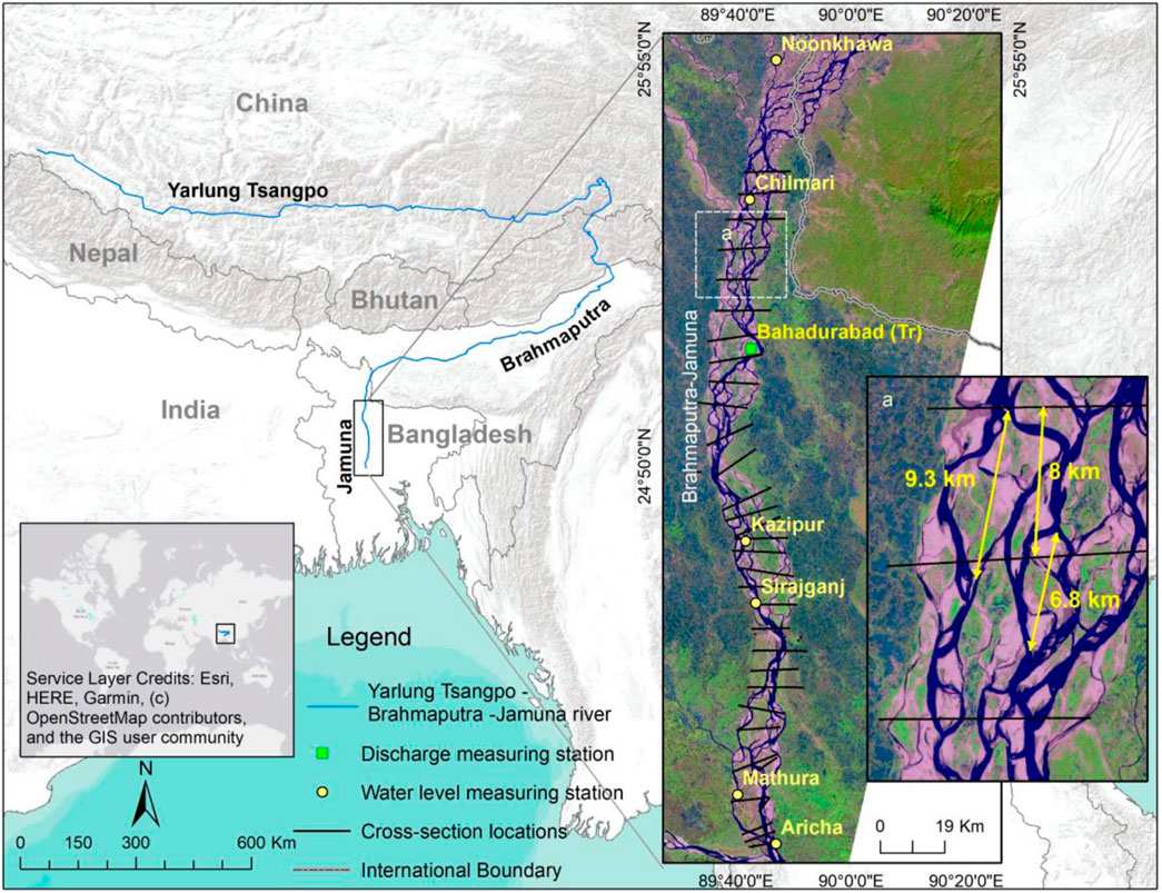
Figure 1. Study area.

Against these backdrops, the goal of this research is to develop an early warning system for riverbank erosion and to field-test this system for the braided Brahmaputra–Jamuna River. The specific objectives were as follows: first, to develop a methodology for bathymetry generation in a data-poor region of the braided Brahmaputra–Jamuna River; second, to evaluate the capability of predicting braided river erosion (in banks and bars) through two-dimensional (2D) numerical modeling; and third, to develop the river erosion prediction web portal and conduct field testing of this system.

2 Study area

The Brahmaputra–Jamuna River, one of the world’s largest braided rivers, has been chosen for this study. The river originates in the Himalayas and flows nearly 1800 km through China (as Tsangpo) and India (as Brahmaputra) before entering Bangladesh, where it takes the name Brahmaputra–Jamuna (Sarker et al., 2014). The current study focuses on the Brahmaputra–Jamuna River flowing through Bangladesh, as depicted in Figure 1. The Brahmaputra Basin covers a catchment area of 560,000 km², with only 8.1% of it located within Bangladesh (Best et al., 2007). The basin undergoes significant morphological variations due to annual rainfall fluctuations, which range from 1,000 mm to 4,000 mm—higher in the Assam floodplains and lower in the upper Tibetan region (Sarma and Acharjee, 2018). Approximately 80% of the annual rainfall occurs during the monsoon season (June–September), resulting in extreme variations in river discharge and sediment transport (Dixit et al., 2023). This hydrological variability influences the river’s morphology by affecting braiding intensity, channel width, and sediment deposition patterns. The bankfull discharge ranges from 45,000 to 60,000 m³/s (FAP, 1995). This river is a major contributor to flooding and erosion in Bangladesh (Hofer and Messerli, 2006; NAWG, 2020). The river discharge is highly seasonal, with maximum flood discharge ranging from 50,000 to 115,000 m³/s over the last five decades (Sarker et al., 2014; Shampa et al., 2022).

The Brahmaputra–Jamuna River exhibits a predominantly braided morphology, characterized by rapid and dynamic bar-channel alterations (Best et al., 2007; Sarker et al., 2014). It has an average width of approximately 10 km, a flow depth of approximately 5–6 m, and a Brice braiding index ranging from 4 to 6 (FAP, 1996).

3 Materials and methods

This study used a 2D hydro-morphological numerical model to predict river erosion, considering both riverbanks and bar regions (Chars) as they became occupied. Table 1 summarizes the data used for system development and verification. Flow boundaries were established using GloFAS seasonal predictions and BWDB time-series discharge and water-level data (1956–2020). Landsat satellite images [red-green-blue (RGB), green, and near-infrared (NIR) bands] from 2019, 2020, 2023, and 2024, along with BWDB cross-sectional data (Figure 1), supported model calibration and validation. Field testing was conducted using measured georeferenced erosion data.

Table 1

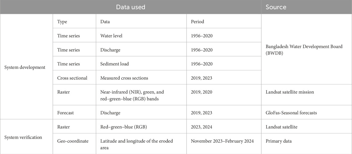
Table 1. Details of the data used in this study.

The methodology (Figure 2) involved selecting a hydrograph from the GloFAS forecast, aligning peak discharge with BWDB data, and defining boundary conditions based on discharge hydrographs and stage-flow and flow-sediment relationships. Model bathymetry was derived from satellite imagery and limited field measurements (Section 3.1). After running the 2D simulation, an erosion hazard map was generated from the final bed-level data. Predictions were disseminated via a web platform integrated with Google Maps Application Programming Interface (API). Further methodological details are provided in the following sections.

Figure 2

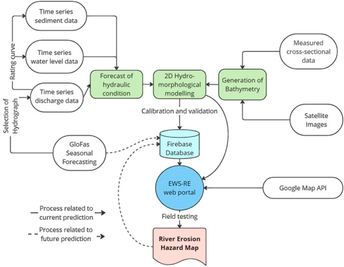
Figure 2. Overall methodology of the study.

3.1 Generation of river bathymetry

3.1.1 Remote sensing-based bathymetry estimation methods

Quantifying braided river morphology is necessary to comprehend their behavior (Williams et al., 2014). The characteristics of the bar-channel confluence and bifurcation play a significant role in determining the river bathymetry. Bar topography and channel bathymetry should, therefore, be included in the process of creating river bathymetry. Assuming log-normal relationships between the water depth $\left(z\right)$ and surface reflectance $R\left({\lambda }_i\right)$ using the band “Blue,” Lyzenga (1978) pioneered the passive water depth measurement method. Although that study provided a theoretical derivation of depth estimation using spectral reflection, empirical adjustment constituted a crucial component of the depth estimation process using the method of Lyzenga (1978). Minimization of such tuning parameters became difficult in regions where data are scarce and aquatic and water quality parameters are difficult to estimate (Stumpf et al., 2003).

Later, Stumpf et al. (2003) introduced the “Ratio” algorithm, in which they scaled the ratio of two spectral bands—band “Blue” and band “Green”—to estimate the flow depth. The linear transformation developed by Lyzenga (1978) showed more variability between atolls and was unable to distinguish depths beyond 15 m. While examining the depth in various types of bathymetries, i.e., spur-and-groove type structures on the forereef, algae-covered pavement, coral-dominated patch and reticulated reefs, and mixture of sand- and coral-dominated reefs, Stumpf et al. (2003) demonstrated that ratio transformation can retrieve depths up to 25 m of water and exhibits enhanced spatial stability. The ratio algorithm is noisier and sometimes fails to detect finer morphological features (smaller than 4–5 pixels) at flow depths of 15–20 m (Stumpf et al., 2003). They used some fixed constants for the considered domain which must be carefully chosen to ensure that, under any condition, the logarithm of reflectance remains positive and that the ratio exhibits a linear response with depth—requirements that are often difficult to meet. Kanno and Tanaka (2012) modified Lyzenga’s predictor coefficients (Lyzenga, 1978), which are relatively less affected by the optical properties of bottom materials and water. Using coral reef images from WorldView-2, they developed and implemented the theoretical fact, illustrating the efficiency of the proposed method. Later, Deng et al. (2008), Jagalingam et al. (2015), and Geyman and Maloof (2019) modified the method proposed by Stumpf et al. (2003) to obtain a positive value after the log conversion and a linear relationship for the ratio and the depth with zero water depth. On the other hand, Williams et al. (2014) demonstrated a surveying technique that uses mobile terrestrial laser scanning and aerial images to create digital elevation models (DEMs) of a 2.5-km stretch of New Zealand’s braided Rees River. They claimed to have modest vertical errors, ranging from 0.03 to 0.12 m in exposed and inundated locations, respectively. Javernick et al. (2014) used the structure-from-motion technique to generate the bathymetry of New Zealand’s braided Ahuriri River. This method requires ground-control and is ideally suited for imagery obtained from non-metric cameras or aerial platforms. However, in the river reach they studied, the depth varied between 0 and 2 m only. Bhuyian and Kalyanapu (2020) presented a methodology using Landsat images, Shuttle Radar Topography Mission (SRTM) DEM, and Multi-Error-Removed Improved-Terrain (MERIT) DEM and assessed water surface elevation, with the braided Jamuna River included as a part of the study. However, the generated bathymetry seems like an average bathymetry of a braided channel unable to produce a variable channel bottom, i.e., the confluence scour. However, to the best of our knowledge, neither of these generated satellite image-based bathymetry has been used for future prediction, i.e., flood or erosion. Furthermore, as a result of climate and anthropogenic changes, the river’s morphological responses change over time. To account for such changes, any bathymetry generation method must be adaptable, and the incorporation of measured data with the remotely sensed data is necessary.

3.1.2 Data fusion approach for bathymetry generation

In this study, we proposed a data fusion technique using a modified ratio algorithm with observed cross-sectional data to provide the initial bathymetry of the braided Brahmaputra–Jamuna River. In this river, where individual braided channel widths range from a few meters to several kilometers, moderate-resolution (30 m) Landsat satellite images were selected to generate bathymetry, optimizing computational efficiency based on the selected grid size.

Here, prior to the estimation of river bathymetry, the channel and bars were separated using the Normalized Difference Water Index (NDWI) developed by Gao (1996). The reflectance values of “green” and “near-infrared” bands were correlated with limited measured data in such a way that represents the channel depth, as shown in Equations 1, 2:

$z=\frac{\left(e^k-e_{\mathit{min}}^k\right)\left(h_{mH}-h_{mL}\right)}{e_{\mathit{max}}^k-e_{\mathit{min}}^k}+h_{mL},(1)$

$k=\frac{R\left({\lambda }_g\right)-R\left({\lambda }_{NIR}\right)}{R\left({\lambda }_g\right)+R\left({\lambda }_{NIR}\right)},(2)$

where the water depth $\left(z\right)$ is expressed as the function of $h_{ml}\text{\hspace{0.17em}and\hspace{0.17em}}{e}^k.$ The value of $k$ is derived using Equation 2. Here, $R\left({\lambda }_g\right)$ and $R\left({\lambda }_{NIR}\right)$ are the atmospherically corrected surface reflectances of “green” and “near-infrared” bands (as shown in Figures 3A,B), respectively, $h_{mL}$ represents the 0.1th percentile of the measured channel depth, and $h_{mH}$ represents the 99th percentile of the measured channel depth (measurement location is shown in Figure 3C). $e$ is Napier’s constant. The “green” and “near infrared” bands from the Landsat 8 satellite in February 2019 were used, as shown in Figures 3A,B, respectively. Later, the water depth was converted to the reduced level by subtracting it from the water level measured during the dry season. For the bar-top topography, Copernicus (COP) DEM (30 m) data were used.

Figure 3

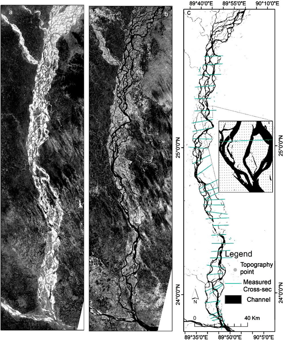
Figure 3. Images used to generate bathymetry. (A) Green band images of Landsat captured on 19th February 2019. (B) NIR band images of Landsat captured on 19th February 2019. (C) Extracted channels.

3.2 Two-dimensional numerical model

3.2.1 Governing equations

The numerical model used in this study was built on the open-source Delft3D platform (version 4.00.01.000000) (Lesser et al., 2004). The model solves shallow water equations derived from Navier–Stokes equations for the incompressible free surface in two-dimensional forms using Boussinesq approximations in the hydrodynamic component. To generate the conservation of mass, continuity Equation 3 was used.

$\frac{\partial h}{\partial t}+\frac{\partial \left(hu\right)}{\partial x}+\frac{\partial \left(hv\right)}{\partial y}=0.(3)$

The conservations of momentum in the x- and y-directions are represented by Equations 4, 5 as follows:

$\frac{\partial u}{\partial t}+u\frac{\partial u}{\partial x}+v\frac{\partial u}{\partial y}+g\frac{\partial \zeta }{\partial x}+\frac{g{n}^2}{{}^3\sqrt{h}}\left(\frac{u\left(u^2+v^2\right)}{h}\right)-v_h\left(\frac{{\partial }^{2}u}{\partial x^2}+\frac{{\partial }^{2}u}{\partial y^2}\right)=0,(4)$

$\frac{\partial v}{\partial t}+u\frac{\partial v}{\partial x}+v\frac{\partial v}{\partial x}+g\frac{\partial \zeta }{\partial x}+\frac{g{n}^2}{{}^3\sqrt{h}}\left(\frac{v\left(u^2+v^2\right)}{h}\right)-v_h\left(\frac{{\partial }^{2}v}{{\partial x}^2}+\frac{{\partial }^{2}v}{{\partial y}^2}\right)=0,(5)$

where h represents the water depth (m); $\zeta$ represents the water level elevation in relation to a datum (here in m PWD); $u\text{\hspace{0.17em}and}v$ are depth average velocity in the x- and y-direction, respectively (m/s); $v_h$ denotes the kinetic eddy viscosity (m²/s); $g$ represents gravity’s acceleration (m/s²); and $n$ symbolizes Manning’s coefficient (sm^−1/3).

The suspended sediment transport, described by the advection–diffusion equation, is determined using Equation 6 as follows:

$\frac{\partial \left(hc\right)}{\partial t}+\frac{\partial \left(huc\right)}{\partial x}+\frac{\partial \left(hvc\right)}{\partial y}=h\left[\frac{\partial }{\partial x}\left(D_H\frac{\partial c}{\partial x}\right)+\frac{\partial }{\partial y}\left(D_H\frac{\partial c}{\partial y}\right)\right].(6)$

Here, $D_H$ represents the horizontal diffusivity, and c is the sediment concentration (kg/m³). For turbulence closure, $k-\epsilon$ turbulence model was used. The bedload sediment transport was calculated using the formula developed by Van Rijn (1993).

Equation 7 was used to obtain the bedload transport rate $\left|{\overline{S}}_{bed}\right|$ as follows:

$\left|{\overline{S}}_{bed}\right|=\left\{\begin{array}{c}0.053\sqrt{\left(s-1\right)g{d}_{50}^3}{D}_{*}^{-0.3}{\left(\frac{{\mu }_c\tau -{\tau }_c}{{\tau }_c}\right)}^{2.1}if\left(\frac{{\mu }_c\tau -{\tau }_c}{{\tau }_c}\right)<〈3.0\\ 0.1\sqrt{\left(s-1\right)g{d}_{50}^3}{D}_{*}^{-0.3}{\left(\frac{{\mu }_c\tau -{\tau }_c}{{\tau }_c}\right)}^{1.5}if\left(\frac{{\mu }_c\tau -{\tau }_c}{{\tau }_c}\right)\ge 3.0\end{array}\right\}.(7)$

In this context, $s$ denotes the specific density of the sediment particle $\left(\frac{{\rho }_s}{{\rho }_f}\right)$, $d_{50}$ indicates the particle size, and $\tau \text{\hspace{0.17em}and\hspace{0.17em}}{\tau }_c$ represent the bed shear stress and critical bed shear stress, respectively. ${\mu }_c$ denotes the ratio of total bed roughness to grain-specific bed roughness. $D_{*}$ represents the dimensionless particle parameter. Equation 8 of mass–balance (Exner, 1925) was used to ascertain the bed elevation in a mixed sediment transport system.

$\left(1-\lambda \right)\frac{\partial {\eta }_{bk}}{\partial t}+m_f\left(\frac{\partial q_{uk}}{\partial x}+\frac{\partial q_{vk}}{\partial y}\right)+m_f\left(E_k-D_k\right)=0.(8)$

Here, $\lambda$ denotes porosity, $q_{uk}\text{\hspace{0.17em}and\hspace{0.17em}}{q}_{vk}$ represent the transport vectors of bedload for size fraction $k$ in two directions, and ${\eta }_{bk}$ signifies the bed-level change attributable to size fraction $k$. The upward and downward suspended sediment transport fluxes near the bed are indicated by $E_k$ and $D_k$, respectively; $m_f$ denotes the morphological acceleration factor. The aggregate of the bed alterations, $\mathrm{\delta }{\eta }_b$, from all size fractions culminates in the overall bed variation in a singular step, as shown in Equation 9:

$\mathrm{\delta }{\eta }_b={\displaystyle \sum _{k=1}^M}\mathrm{\delta }{\eta }_{bk}.(9)$

Here, M represents the total size fraction, which is considered 1.

Using the method developed by Roelvink et al. (2006), the erosion flux is redistributed from a wet cell to the nearby dry cells in cases where adjoining dry cells (close to the bank or bar) possess the condition of erosion. ${\theta }_{dc,thr}$, the actual fraction of erosion at an edge, can be articulated as follows: if ${\theta }_{dc,thr}$ denotes the greatest erosion fraction and $h_{dcmax}$ represents the designated water depth in the wet cell for the complete reallocation of ${\theta }_{dc,thr}$, then ${\theta }_{dc}$ can be expressed as shown in Equation 10:

${\theta }_{dc}=\mathit{min}\left(\frac{h-h_{dc,thr}}{h_{dcmax}-h_{dc,thr}},1\right){\theta }_{dc,thr}.(10)$

Here, in a dry cell, $h_{dc,thr}$ denotes the minimal threshold flow depth required for the reallocation of erosion.

3.2.2 Model schematization

A 250-km-long curvilinear grid, with an average width of 44 km, was created for the Brahmaputra–Jamuna numerical model, commencing 10 km upstream of the Noonkhawa water level observation station and ending near the Aricha water level measurement station, as illustrated in Figure 4. The reach was separated using a grid of 594 × 189 cells. Bar sizes varied from 549.83 × 205 m² to 28635 × 10475 m² within the span of the Brahmaputra–Jamuna River (Shampa, 2019). The selected grid resolution guarantees that a minimum of two grid cells (450 × 140 m²) encompass each bar. All the base parameters are listed in Table 2, together with the corresponding references based on which the parameters were established. In this study, Manning’s roughness coefficient was set at 0.027 as the whole braided plain may become submerged during the monsoon, according to FAP (1995). The mean sediment size was considered 200 µm (Kabir and Ahmed, 1996; Nakagawa et al., 2013). Discharge and water level data from 2019, collected from BWDB, were used as the boundary conditions, as shown in Figure 5. The model was calibrated using data from measured water levels. Figure 6 illustrates three instances of spatial calibration during the pre-monsoon, monsoon, and post-monsoon periods, wherein the simulated water levels were compared to actual water levels at five monitoring sites (from upstream to downstream). Manning’s roughness, Van Rijn’s reference height factor, and the morphological acceleration factor are used as calibration parameters. The chosen values of these parameters are enumerated in Table 2. The mean absolute error (MAE) (Willmott and Matsuura, 2005) method was used during the calibration process. Upon completion of the calibration, the MAE values for Noonkhawa, Chilmari, Bahadurabad, Sirajganj, and Mathura were 0.315, 1.269, 1.290, 0.229, and 0.489, respectively.

Figure 4

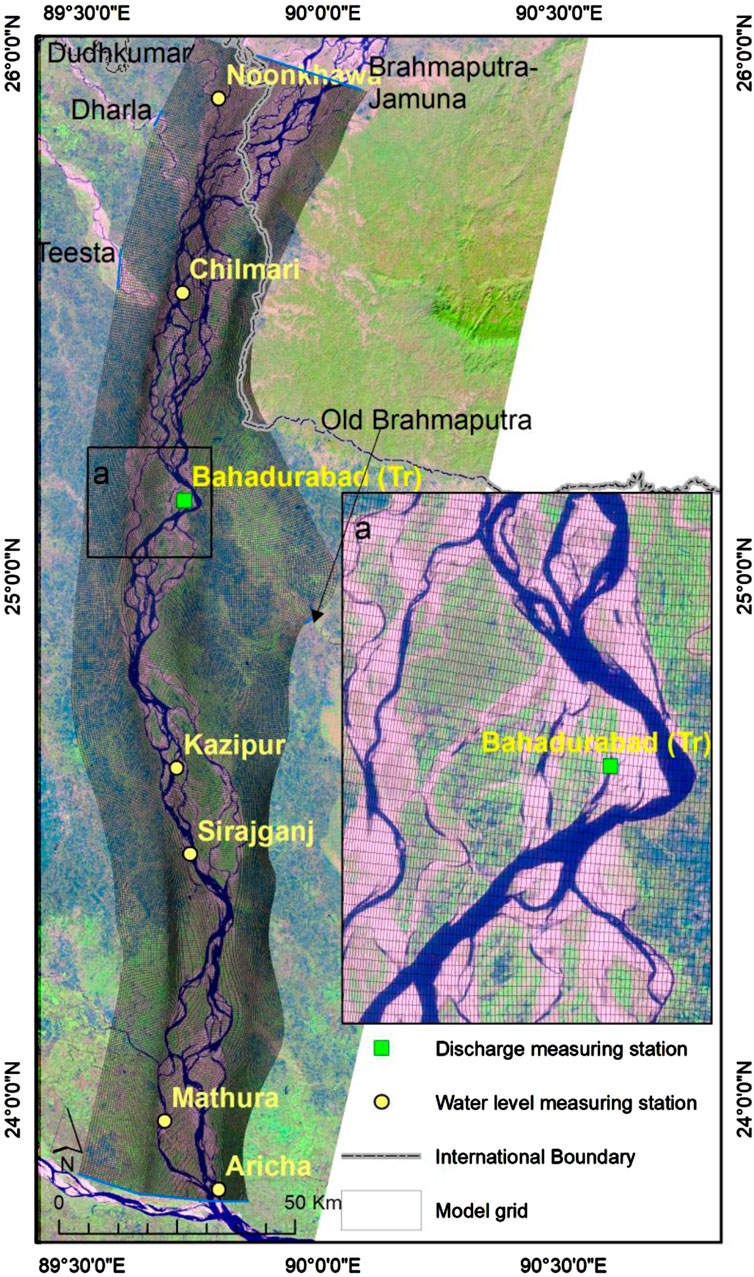
Figure 4. Model grid and boundary location.

Table 2

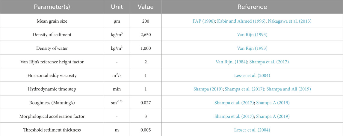
Table 2. Base parameters of the model.

Figure 5

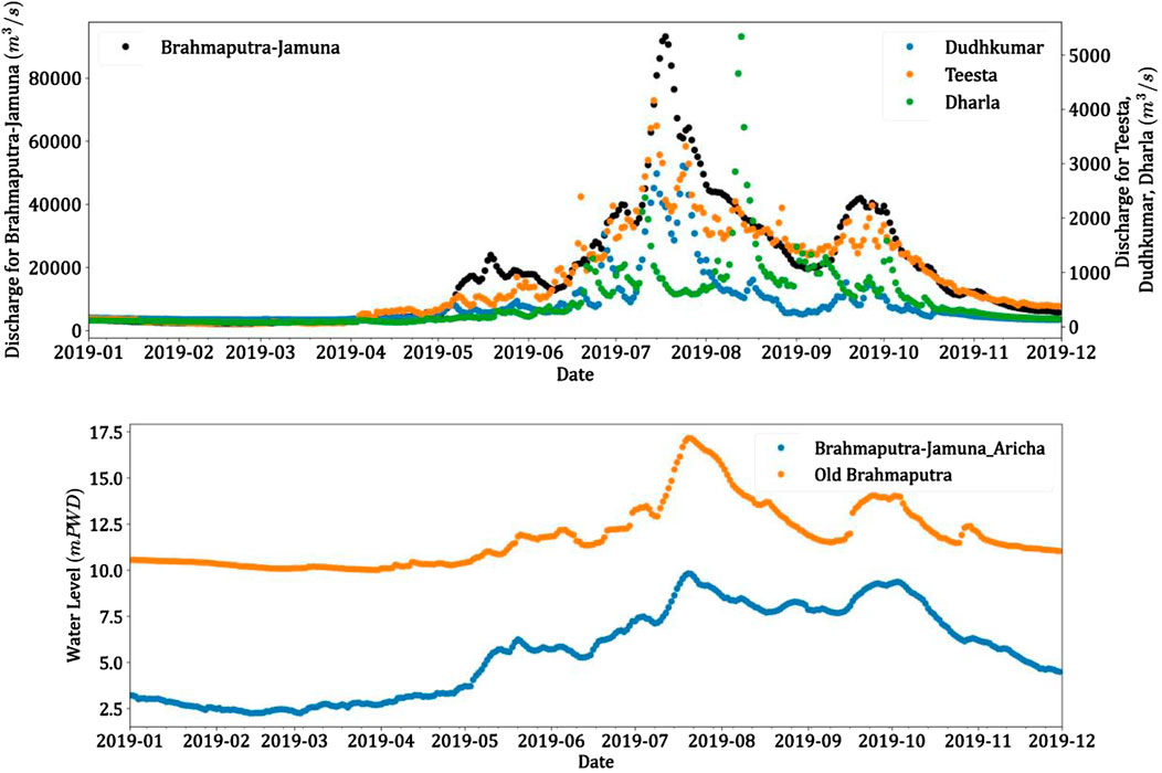
Figure 5. Boundary conditions of the mode for the year 2019. Discharge boundary conditions (top) and the water-level boundary condition (bottom).

Figure 6

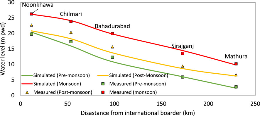
Figure 6. Spatial calibration of the water level.

3.2.3 Accuracy assessment

Several statistical tests were performed to evaluate the accuracy of the simulated water level and discharge results, including the Nash–Sutcliffe efficiency (NSE) coefficient, percent bias (PBIAS), relative root mean square error (RRMSE), and coefficient of determination, R², using Equations 11–14. Here, $X_0^i$ represents the $i^{th}$ observed value of the X parameter, and $X_s^i$ represents the $i^{th}$ simulated value of the X parameter. $n$ is the total number of observations, and $X_o^{avg}$ represents the average value of X parameter’s observed data. Table 3 lists the performance ratings mentioned in previous studies (Despotovic et al., 2016; Moriasi et al., 2007). For the parameter where the number of measurements was insufficient to make a statistical comparison, we used a visual comparison rather than a statistical test.

$\mathit{N}\mathit{S}\mathit{E}=1-\left(\frac{{\displaystyle {\sum }_{i=1}^n}{\left({\mathit{X}}_0^{\mathit{i}}-{\mathit{X}}_{\mathit{s}}^{\mathit{i}}\right)}^2}{{\displaystyle {\sum }_{i=1}^n}{\left({\mathit{X}}_0^{\mathit{i}}-{\overline{\mathit{X}}}_0\right)}^2}\right),(11)$

$\mathit{P}\mathit{B}\mathit{I}\mathit{A}\mathit{S}=100*\left(\frac{{\displaystyle {\sum }_{\mathit{i}=1}^{\mathit{n}}}{\mathit{X}}_0^{\mathit{i}}-{\mathit{X}}_{\mathit{s}}^{\mathit{i}}}{{\displaystyle {\sum }_{\mathit{i}=1}^{\mathit{n}}}{\mathit{X}}_0^{\mathit{i}}}\right),(12)$

$RRMSE=\frac{\sqrt{\left(\frac{1}{n}{\displaystyle {\sum }_{i=1}^n}{\left(X_o^i-X_s^i\right)}^2\right)}}{{\displaystyle {\sum }_{i=1}^n}{X}_o^i}*100,(13)$

${\mathit{R}}^2=1-\frac{{\displaystyle {\sum }_{\mathit{i}=1}^{\mathit{n}}}{\left({\mathit{X}}_{\mathit{o}}^{\mathit{i}}-{\mathit{X}}_{\mathit{s}}^{\mathit{i}}\right)}^2}{{\displaystyle {\sum }_{\mathit{i}=1}^{\mathit{n}}}{\left({\mathit{X}}_{\mathit{o}}^{\mathit{i}}-{\mathit{X}}_{\mathit{o}}^{\mathit{a}\mathit{v}\mathit{g}}\right)}^2}.(14)$

Table 3

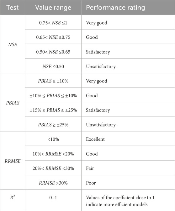
Table 3. General performance ratings for several statistics.

To assess the accuracy of the eroded location, we used the confusion matrix, and the accuracy was determined using the kappa statistics proposed by Monserud and Leemans (1992). In this study, 100 ground truth points were generated in the classified image using the stratified random sampling method to estimate accuracy. The following Equations 15–17 are used to identify accurate kappa statistics:

$\text{kappa\hspace{0.17em}coefficient}=\mathrm{N}{\displaystyle \sum _{r=1}^r}{n}_{ii}-{\displaystyle \sum _{r=1}^r}\left(n_{icol}{n}_{irow}/N^2\right)-{\displaystyle \sum _{r=1}^r}{n}_{icol}{n}_{irow},(15)$

$\text{producer}\prime \mathrm{s}\text{\hspace{0.17em}accuracy}=n_{ii}/n_{i\mathit{r}\mathit{o}\mathit{w}},(16)$

$\text{user}\prime \mathrm{s}\text{\hspace{0.17em}accuracy}=n_{ii}/n_{icol},(17)$

where $i$ is the class number, N represents the total number of classified values versus truth values, $n_{ii}$ is the number of truth class $i$ values that have also been classified as class $i$, $n_{icol}$ denotes the total number of predicted values, and $n_{irow}$ represents the total number of truth values in class $i$. If the number of correctly identified eroded locations is $T_e$, the number of correctly identified non-eroded location is $T_{ne}$, the number of incorrectly identified eroded locations is $F_e$, and the number of incorrectly identified non-eroded locations is $F_{ne}$, then the overall accuracy and sensitivity are calculated using Equations 18, 19, respectively, as follows:

$Overallaccuracy=\frac{T_e+T_{ne}}{T_p+T_{ne}+F_e+F_{ne}},(18)$

$Sensitivity=\frac{T_e}{T_e+F_{ne}}.(19)$

3.3 Boundary conditions

To simulate the numerical model, upstream (often discharge) and downstream boundary conditions (e.g., water level) are required. The magnitude of flow and shape of the flow hydrograph are both crucial factors for the river’s morphological transition. The magnitude of flow was estimated using GloFAS-Seasonal forecasts. For streamflow projections, the GloFAS-Seasonal forecasts usually combine ECMWF’s seasonal meteorological forecasts, SEAS5, with the Lisflood river routing model (Alfieri et al., 2013; Chen et al., 2019; Emerton et al., 2018). It provides the average river flow on a weekly basis, with a lead term of 4 months. The first component is the meteorological data derived from SEAS5, which uses a data assimilation system in conjunction with a global circulation model. The second model component is a modified Hydrology Tiled ECMWF Scheme of Surface Exchanges over Land (HTESSEL), which quantifies the land surface response to atmospheric forcing, considering moisture content, soil temperature, and snowpack conditions across the forecast period (Balsamo et al., 2011). The third component, Lisflood, simulates groundwater dynamics and flood routing via the river network. An example of such forecasts is shown in Figure 7A, which represents the GloFAS-Seasonal forecasts for June to September 2024 for the Bahadurabad station. A 90th percentile of river discharge was selected from this seasonal estimate as the projected peak discharge. The peak discharge was compared to the historical weekly hydrograph of the Brahmaputra–Jamuna River, as shown in Figure 7B, and the most recent corresponding hydrograph shape was selected. Sometimes, the peak needs to be adjusted, and the adjustment was performed according to Shampa et al. (2018). To generate the downstream boundary condition, the corresponding measured water level of Aricha was used.

Figure 7

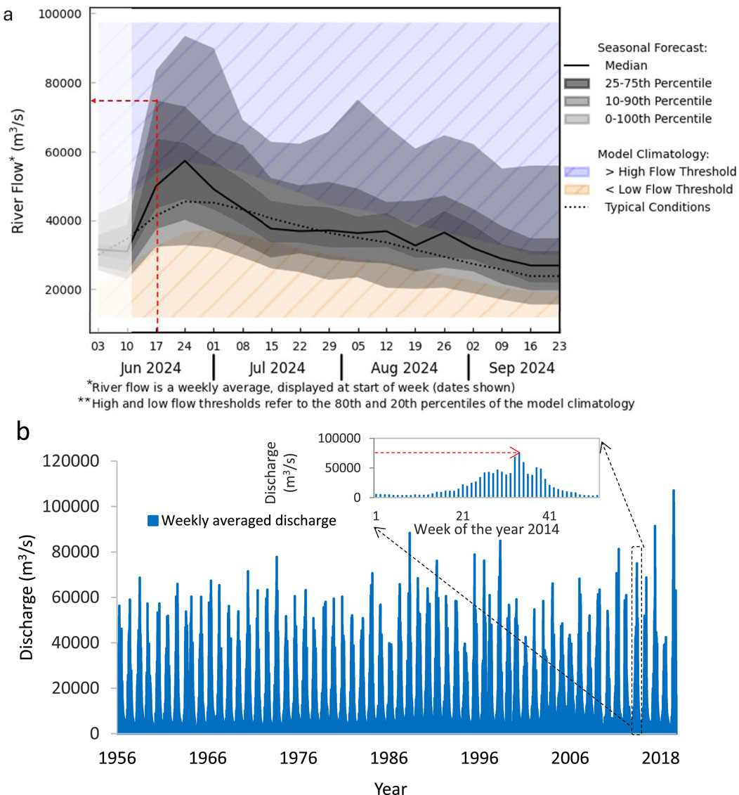
Figure 7. Selection of boundary conditions for EWS-RE. (A) Seasonal forecasts by GloFAS. (B) Weekly averaged discharge of Brahmaputra–Jamuna at Bahadurabad.

3.4 Determination of early warning thresholds

If the flow depth in any grid cell, $h_{\left(x,y\right)}$ is greater than 0 at time $t=i$, the early warning for that cell is determined based on the condition given in Equation 20 as follows:

$\frac{{\left({\eta }_{\left(x,y\right)}\right)}_{t=0}-{\displaystyle \sum _{t=0}^{t=i}}\mathrm{\delta }{\eta }_{b_{\left(x,y\right)}}}{\frac{1}{n_g}{\displaystyle \sum _{g=1}^{n_g}}\left[{\left({\eta }_{\left(x,y\right)}\right)}_{t=0}-{\left({\eta }_{\left(x,y\right)}\right)}_{t=i}\right]}\ge 0.5,\text{when}{h}_{\left(x,y\right)}>0.(20)$

Here, ${\left({\eta }_{\left(x,y\right)}\right)}_{t=0}$ represents the initial bed elevation of the grid cell at $t=0$, ${\left({\eta }_{\left(x,y\right)}\right)}_{t=i}$ represents the bed elevation of the grid cell at $t=i$, and $n_g$ is the number of grid cells, where $h_{\left(x,y\right)}>0$. This condition helps in assessing the stability of the riverbank and triggering an early warning when significant bed elevation changes occur over time.

3.5 Framework of the web warning system

A website was developed to implement the early warning system for river erosion (EWS-RE), displaying erosion-prone zones using Google Maps’ JavaScript API. The client-side application was built using React.js, while the backend was developed using Express.js and Firebase. The platform (www.ews-re.com) functions as a third-party web application, querying and interacting with Google Maps via API calls. The system uses global functions and React hooks to manipulate the 2D map view, retrieve viewport data, and integrate GeoJSON features for representing geographic elements like polygons. To ensure compatibility with Google Maps, all data are converted into the GeoJSON format before visualization.

Figure 8 illustrates the architecture of the EWS-RE web portal, which integrates a backend server and Google Maps API to disseminate river erosion warnings. In this system, Google Maps acts as the API provider, while the backend server manages data distribution. The website is hosted on a web server. The client-side application communicates with the backend via REST API, which retrieves data from the database in the GeoJSON format. These data are then sent to Google Maps to render real-time hazard maps, with color-coded polygons indicating different warning levels. Users can select water levels and search locations, while the database is managed via an admin portal, where GeoJSON files are uploaded with relevant attributes like year and water level.

Figure 8

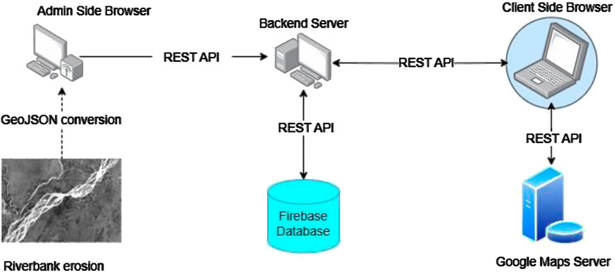
Figure 8. Architecture of the EWS-RE web portal.

Figure 9 presents a snapshot of the EWS-RE web portal interface. The left half features the functional palette, while the right half displays the 2D viewport. This application system comprises three functional modules, each detailed from function introduction to implementation technique as follows:

1. Searching and location: This module enables users to accurately locate positions on the three-dimensional (3D) digital globe by inputting the name of a place, resulting in an automatic adjustment of the view to the designated location. This function is executed through a special interface of the Maps JavaScript API. Geocoding services for location finding are provided by Google Maps.

2. River erosion alerts for specific years: This is the primary functional module of the application, where forecasters can issue three types of river erosion warnings on the local server, which are then displayed in varying colors to indicate high-, medium-, and low-erosion susceptibility zones. This erosion category assessment is based on the simulation results on anticipated boundary conditions using the natural breaks algorithm described by Jenks (1967). For example, for the year 2024, if degradation in the final bed level compared to the starting bed level was less than 0.05 m, 0.05 m–0.73 m, or greater than 0.73 m in each grid cell, it is classified as low-, moderate- and high-erosion zones, respectively.

3. River erosion at a specified water level: Clients can input a specific water level from the Bahadurabad station, and these data will be converted to the corresponding discharge based on the anticipated hydrograph, enabling users to identify areas susceptible to river erosion.

Figure 9

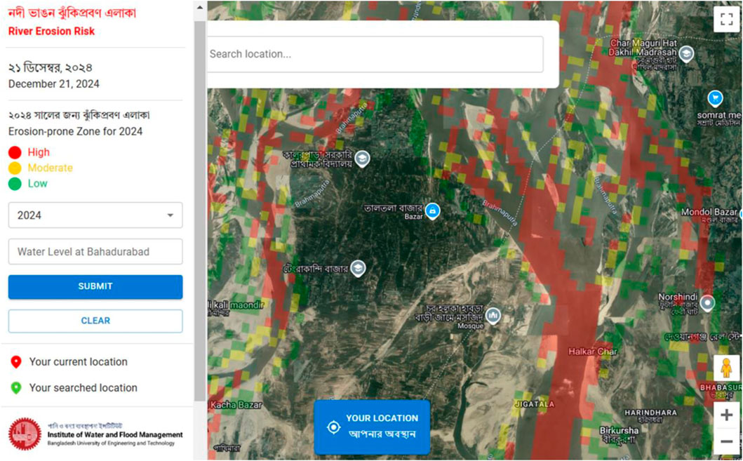
Figure 9. Visualization of the EWS-RE web portal.

4 Results

4.1 Generated initial bathymetry

Figure 10 depicts generated bathymetry created using the methods described in Section 3.1. The elevation ranges from 38 m PWD to −10 m PWD, and the channel depth ranges from 3 to 14 m. The braided channel’s average depth was found to be 6.08 m. This figure shows that generated bathymetry had depth variations due to confluence and bifurcations. The frequency distribution of channel depths is depicted in Figure 11. This figure indicates that most of the channel depth ranges between 3.5 and 9.5 m. The subplots of Figure 10 show the comparison of generated bathymetry and measured data. The sec A–A and sec B–B were located nearly 8.5 km downstream of the Bahadurabad station and 19.5 km from the Sirajganj water level measuring station, respectively. The four channels were observed from the measured data in the case of secA–A. In those channels, the maximum reduced levels were 7.2, 7.8, 6.5, and 4.8 m PWD. The generated elevations along the same location were 4.1, 6.3, −1.87, and 4.8 m PWD, respectively. In the case of sec B–B, two channels were observed from the measured data, with elevations of 3.05 and −4.16 m PWD and elevations of 3.21 and −4.52 m PWD generated. The average vertical deviation in these locations was nearly 2 m. Figure 12 shows the relationship between the estimated and measured reduced levels. It shows a positive correlation with a coefficient of determination of 0.756. However, it should be noted that this bathymetry served as the initial condition and was updated at each timestep during the simulation.

Figure 10

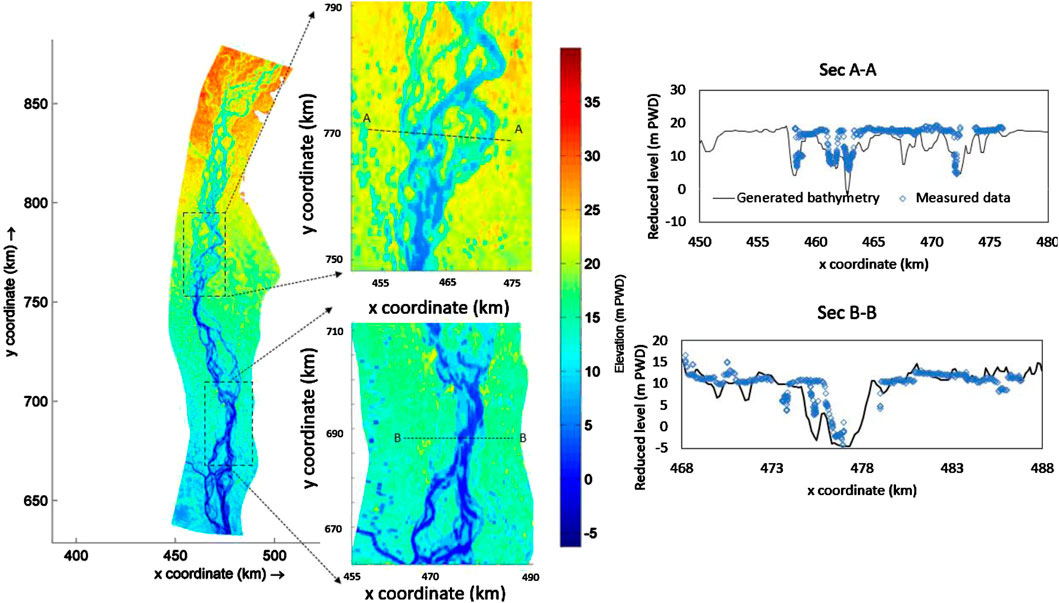
Figure 10. Generated bathymetric elevation of the year 2019.

Figure 11

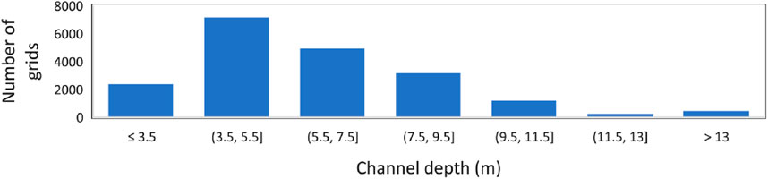
Figure 11. Frequency distribution of channel depths.

Figure 12

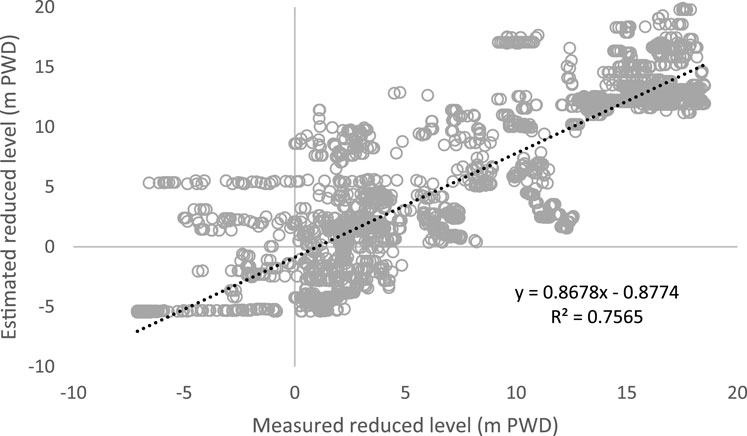
Figure 12. Relationship between the measured and estimated bathymetries.

4.2 Comparisons of measured and simulated hydraulic characteristics

The simulated discharge was compared to the measured data at the Bahadurabad station, which is the reach’s only discharge-measuring station. The water levels in Noonkhawa, Chilmari, Bahadurabad, Sirajganj, and Mathura were compared. The evaluation statistics, i.e., NSE, PBIAS, RRMSE, and R² values, are shown in Table 4. In hydrology, previous researchers mentioned that the NSE value should be greater than 0.5, while PBIAS should be within ±25% to be satisfactory (Knoben et al., 2019; Moriasi et al., 2007; Vijai et al., 1999). RRMSE should be within 10% to be considered acceptable, according to Despotovic et al. (2016). These values were within the acceptable range.

Table 4

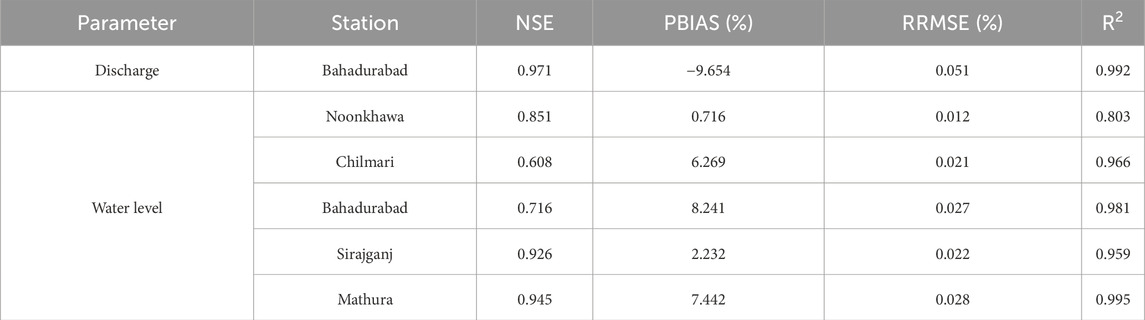
Table 4. Evaluation statistics for discharge and water levels.

In the study reach, BWDB only measured the velocity along the Bahadurabad section, and for the year 2019, only 25 records were available. These were cross-sectional maximum velocity measurements, which were not directly comparable to simulation outputs. Figure 13 depicts the relationship between measured maximum velocity and simulated depth average velocity as a function of the water level. When the water level was low (12–14 m PWD in March and April), higher velocities were observed, which could be due to flow localization, a phenomenon common in a mighty river like this.

Figure 13

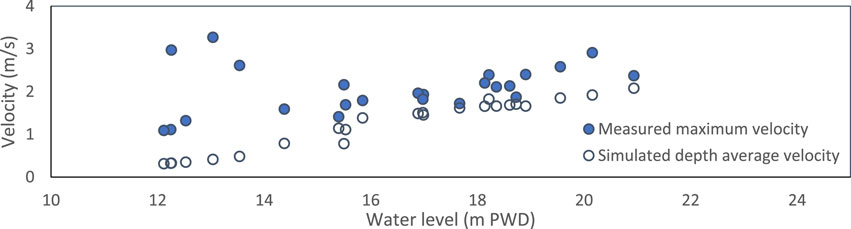
Figure 13. Variation in velocity with the water level at Bahadurabad.

Only 21 dates were available for year-round measured sediment discharge data. Figure 14 depicts the difference between measured and simulated sediment discharges. Sediment loads measured in this study range from 0 to 506,039 kg/s, with an average of 76,466 kg/s. The sediment loads simulated range from 0.275 to 900,686 kg/s, with a yearly average load of 64,751 kg/s.

Figure 14

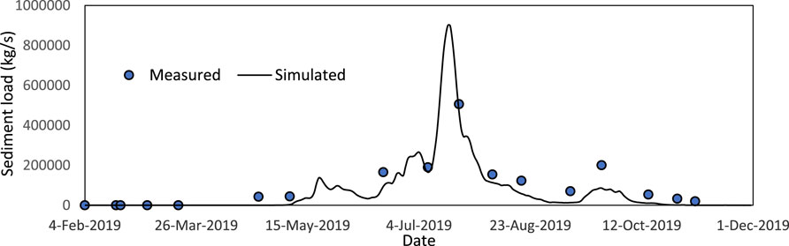
Figure 14. Variation in measured and simulated sediment discharges.

4.3 Spatial erosion

The model-generated riverbed evolution is shown in Figure 15. At the end of the simulation, several braiding characteristics (e.g., formation of new braided channels, alterations in bar’s shape and size, and lateral channel migration) were observed. However, Figure 16 shows the comparison between satellite image-driven and simulated spatial erosion. The actual erosion was 336.506 sq. km, while in the model, it was 378.39 sq. km. As our aim was only to estimate the probable erosion location (not the volume), a confusion matrix of erosion was created by comparing only the eroded locations (Table 5). In this study, the kappa cofficient was 73.3%, which is a “very good” agreement (70%–85%) according to Monserud and Leemans (1992). The sensitivity and confidence level of the EWS-RE prediction (at z = 1.95996) were determined to be 88% and 95%, respectively.

Figure 15

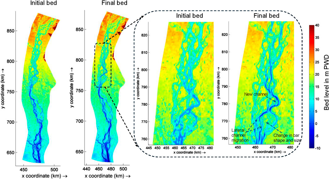
Figure 15. Model-generated evolution of the riverbed for the year 2019.

Figure 16

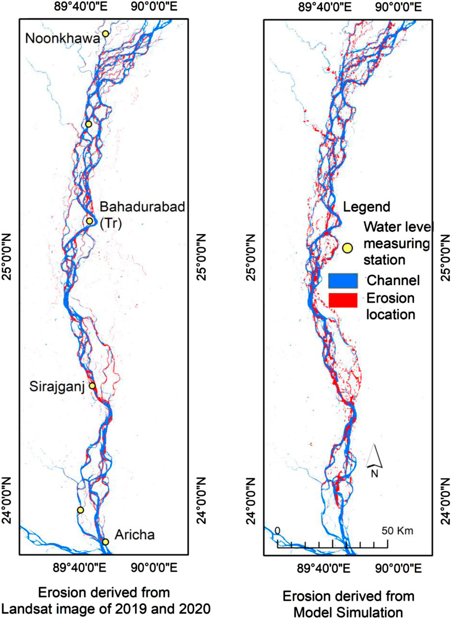
Figure 16. Comparison between satellite image-driven and simulated spatial erosion.

Table 5

Table 5. Accuracy assessment of spatial erosion location.

4.4 Field testing of erosion early warning

The erosion early warning system was validated using an annual projection of the hydrologic conditions for 2023. The projected erosion was tested in 81 places, with the river divided into three sections, namely, upstream (near Noonkhawa), middle (near Kazipur), and downstream (near Aricha), as illustrated in Figure 17. The locations of eroding banks were collected between November 2023 and February 2024. The comparison of actual and predicted erosion location is listed in Table 6. The overall accuracy along the river was 70%. The lowest accuracy (67%) was found in the middle reach, particularly in the bank-attached channel segment where severe erosion was expected. Satellite image analysis revealed erosion areas of 24.4 km², 63.5 km², and 3.8 km² at Noonkhawa, Kazipur, and Aricha, respectively, while the EWS-RE predictions indicated 33.2 km², 81.2 km², and 3.1 km² for the same locations. Among the accurately identified eroded sites, 68.8% were situated in high-erosion zones, 31.3% in moderate-erosion zones, and 0.0% in low-erosion zones.

Figure 17

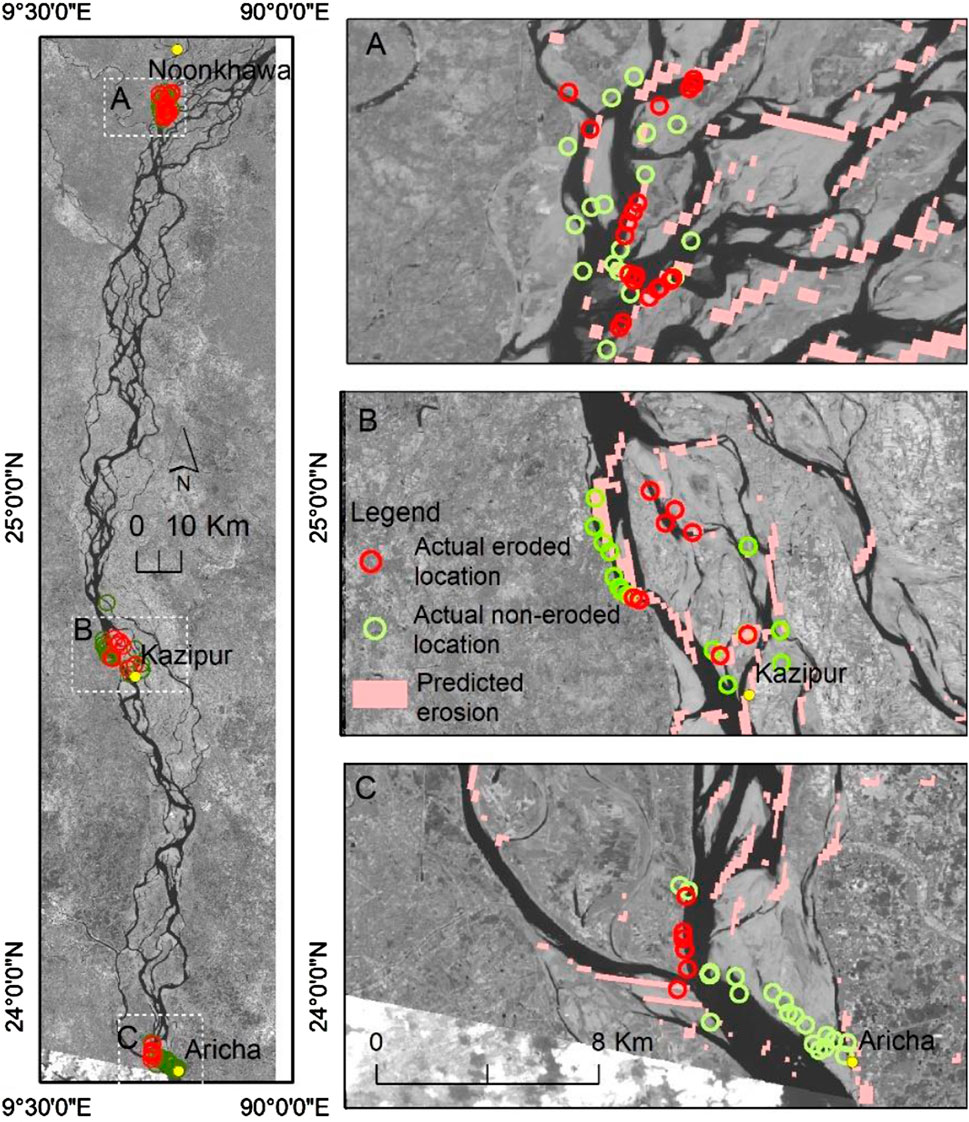
Figure 17. Field testing location of the prediction for the monsoon erosion of the year 2023. The background image shows the end of monsoon channel assignment (Landsat image of February 2024).

Table 6

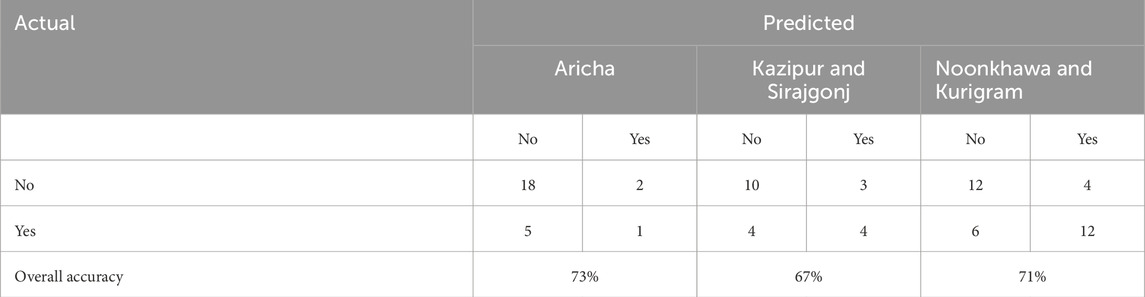
Table 6. Erosion prediction accuracy assessment of field-testing locations.

5 Discussion

Riverbank erosion, regarded as a significant natural hazard in a densely populated and land-scarce country such as Bangladesh, is vital to fluvial, estuarine, and coastal dynamics, encompassing various geographical and temporal dimensions, with considerable physical, ecological, and economic ramifications (Zhao et al., 2022). Any riverbank protection measures modify the river’s hydro-morphology and entail ecological repercussions, in addition to substantial costs. Early warnings of riverbank erosion could significantly influence the trade-off between the choice of structural protection and nature-based solutions, such as permitting bank erosion and the relocation of communities and assets. The EWS-RE developed through this study may play a significant role in this context as a soft solution measure.

CEGIS (2019) identified four erosion-prone sites on the right bank and 10 on the left bank. The analogous four right bank positions were also observed in our forecasts. Our projections along the left bank diverge from CEGIS at three points, with actual erosion detected at one of these sites. It is important to note that CEGIS did not provide predictions for the entire banklines, including the bars, whereas our predictions encompass these areas (Figure 16). CEGIS (2023) reported no erosion forecasts at our field-testing locations. We noticed significant erosion within the braided belt in the upstream portion. The erosion within the braided belt, especially bar areas, was not previously documented in the literature, but Marra et al. (2014) and Rashid and Habib (2022) indicated a higher braided index in the upstream section of the river. Higher braided index values indicate greater morphological activity (e.g., erosion and accretion), which is consistent with our observations. Most bank erosion occurred in the middle reach (Bahadurabad to Sirajganj). This finding is consistent with previous studies, such as Sarker et al. (2014) or Rashid and Habib (2022), as the current westward migration trend was stronger in those areas.

However, field testing revealed an overall prediction accuracy of 70%. In the false-positive areas, numerous hard bank protection structures (as shown in Figure 18) were identified, effectively preventing lateral bank displacement. In contrast, the false-negative regions corresponded to erosion in secondary or tertiary channels, which were initially narrow before the monsoon season. These channels were not well-represented in the numerical model due to limitations in grid resolution.

Figure 18

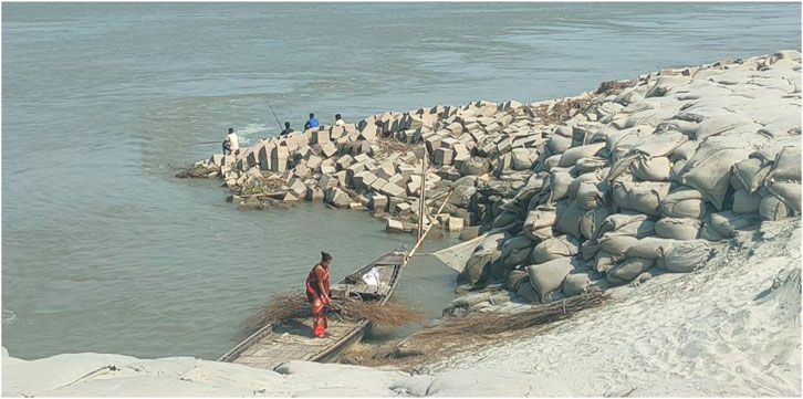
Figure 18. Geo-bags and CC blocks are used to protect the riverbank near Kazipur.

In addition, one of the purposes of this research is to generate bathymetry for the ungagged area of one of the world’s largest braided rivers, the Brahmaputra–Jamuna. There is evidence of reproducing a portion of the river (Bhuyian and Kalyanapu, 2020), but testing the generated bathymetry in spatial erosion prediction using a numerical model was not available, to the best of our knowledge. We found that when used as an input to numerical modeling, the generated bathymetry can reproduce spatial erosion phenomena with a certain level of accuracy. The accuracy of the estimation can be improved by using finer bathymetry and grid. The channel depth in our generated bathymetry ranges from 3 to 14 m. FAP (1995) measured the hydraulic depth from 3.8 to 6.6 m. However, higher depths were observed near hydraulic structures (e.g., spurs) or near bars, ranging from 9 to 14 m (Ashworth et al., 2000; Zhang et al., 2011). As a result, we can say that our estimates were within the observable range.

In this study, the river was mathematically reconstructed using two-dimensional morphological modeling. Some features (for example, hydraulic structures such as spurs) produce a three-dimensional flow that was not fully captured here. It is one of the major limitations of this study. Our analysis focused exclusively on surface flow erosion. However, erosion may also occur owing to seepage or geotechnical reasons, which we could not incorporate. In the case of braided rivers, where frequent bank erosion occurs along the riverbanks and bar areas, the incorporation of a fully dynamic bank erosion model significantly increases the computing efforts of the system.

6 Conclusion

Erosion and accretion within braided rivers, driven by channel realignment and bar dynamics, are natural processes. The distinctive behavior of braided rivers generates issues when erosion occurs in areas inhabited by humans. To address this, we developed an early warning system (EWS-RE) to predict and mitigate erosion risks. Our study highlights the critical need for high-resolution river bathymetry in data-scarce regions and proposes a data fusion approach that integrates satellite imagery with limited field observations as baseline data for morphological simulations. The numerical simulation demonstrated that bathymetry generated using this method was sufficient for accurately estimating flow hydraulics when applied with appropriate boundary conditions. The average depth of the braided channel during the 2019 monsoon was determined to be 6.08 m, aligning with the river’s average depth in a typical hydrologic year. Model validation against observed flow characteristics at one discharge station and five water level stations yielded satisfactory results. Key performance metrics—NSE, PBIAS, RRMSE, and R²—were all within acceptable hydrological thresholds. NSE values ranged from 0.60 to 0.97, PBIAS remained within ±10%, RRMSE remained below 0.05%, and R² ranged from 0.80 to 0.99, confirming the model’s reliability. The spatial erosion accuracy was determined to be 88%. The sensitivity and confidence level of the EWS-RE prediction were established at 88% and 95%, respectively. The field testing of the warning indicated an accuracy of 70% along the river. Despite the inherent complexities of predicting riverbank erosion, we believe that our findings provide valuable insights for sustainable river management. By enhancing predictive capabilities in braided river systems, this study contributes to the development of more effective mitigation strategies, ultimately supporting disaster risk reduction and resilience-building efforts in vulnerable regions.

Data availability statement

The raw primary data supporting the conclusions of this article will be made available by the authors, without undue reservation with on request.

Author contributions

S: conceptualization, formal analysis, funding acquisition, investigation, validation, writing – original draft, and writing – review and editing. HM: data curation, formal analysis, project administration, validation, and writing – review and editing. IN: formal analysis, investigation, and writing – review and editing. MH: methodology and writing – review and editing. AB: software and writing – original draft. NA: software and writing – review and editing. FA: software and writing – review and editing. SB: software and writing – review and editing. MI: investigation and writing – review and editing.

Funding

The author(s) declare that financial support was received for the research and/or publication of this article. This work was supported by the ICT division of Government of Bangladesh under the innovation grant.

Acknowledgments

The authors express their gratitude to the Ministry of Science and Technology of Government of Bangladesh for their initial funding to start this research. The authors also express their gratitude to Prof. Dr. M. Sohel Rahman, Department of Computer Science and Engineering (CSE), Bangladesh University of Engineering and Technology (BUET), for his support to the project.

Conflict of interest

The authors declare that the research was conducted in the absence of any commercial or financial relationships that could be construed as a potential conflict of interest.

Generative AI statement

The authors declare that no Generative AI was used in the creation of this manuscript.

Publisher’s note

All claims expressed in this article are solely those of the authors and do not necessarily represent those of their affiliated organizations, or those of the publisher, the editors and the reviewers. Any product that may be evaluated in this article, or claim that may be made by its manufacturer, is not guaranteed or endorsed by the publisher.

References

Alfieri, L., Burek, P., Dutra, E., Krzeminski, B., Muraro, D., Thielen, J., et al. (2013). GloFAS-global ensemble streamflow forecasting and flood early warning. Hydrol. Earth Syst. Sci. 17, 1161–1175. doi:10.5194/hess-17-1161-2013

CrossRef Full Text | Google Scholar

Ashworth, P. J., Best, J. L., Roden, J. E., Bristow, C. S., and Klaassen, G. J. (2000). Morphological evolution and dynamics of a large, sand braid-bar, Jamuna River, Bangladesh. Sedimentology 47, 533–555. doi:10.1046/j.1365-3091.2000.00305.x

CrossRef Full Text | Google Scholar

Balouchi, B., Rüther, N., and Schwarzwälder, K. (2024). Temporal variation of braided intensity and morphodynamic changes in a regulated braided river using 2D modeling and satellite images. River Res. Appl. 40, 708–724. doi:10.1002/rra.4268

CrossRef Full Text | Google Scholar

Balsamo, G., Pappenberger, F., Dutra, E., Viterbo, P., and van den Hurk, B. (2011). A revised land hydrology in the ECMWF model: a step towards daily water flux prediction in a fully-closed water cycle. Hydrol. Process 25, 1046–1054. doi:10.1002/hyp.7808

CrossRef Full Text | Google Scholar

Best, J. L., Ashworth, P. J., Sarker, M. H., and Roden, J. E. (2007). “The Brahmaputra-Jamuna River, Bangladesh,” in Large rivers: geomorphology and management. Editor A. Gupta (John Wiley and Sons), 395–430.

CrossRef Full Text | Google Scholar

Bhuyian, M. N. M., and Kalyanapu, A. (2020). Predicting channel conveyance and characterizing planform using river bathymetry via satellite image compilation (RiBaSIC) algorithm for DEM-based hydrodynamic modeling. Remote Sens. (Basel) 12, 2799. doi:10.3390/rs12172799

CrossRef Full Text | Google Scholar

Bryant, S., and Mosselman, E. (2017). “Taming the Jamuna: effects of river training in Bangladesh,” in NCR days 2017, Book of abstracts. Editors A. J. F. Hoitink, T. V. de Ruijsscher, T. J. Geertsema, B. Makaske, J. Wallinga, J. H. J. Candelet al. 1st Edn. Wageningen, Netherlands: NCR, 114.

Google Scholar

CEGIS (2019). Prediction of riverbank erosion along the Jamuna, Ganges and Padma river in 2019.

Google Scholar

CEGIS (2023). Annual report for 2023 erosion prediction along the Jamuna, the Ganges and the Padma rivers. 1st Edn. Dhaka, Bangladesh: Center for Environmental and Geographic Information Services.

Google Scholar

Chen, K., Guo, S., Wang, J., Qin, P., He, S., Sun, S., et al. (2019). Evaluation of GloFAS-Seasonal forecasts for cascade reservoir impoundment operation in the upper Yangtze river. Water (Switzerland) 11, 2539. doi:10.3390/w11122539

CrossRef Full Text | Google Scholar

Deng, S., Xia, J., Zhou, Y., Zhou, M., and Zhu, H. (2024). Prediction and early-warning of bank erosion in the middle Yangtze River, China. Catena (Amst) 242, 108105. doi:10.1016/j.catena.2024.108105

CrossRef Full Text | Google Scholar

Deng, Z., Ji, M., and Zhang, Z. (2008). Mapping bathymetry from multi-source remote sensing images: a case study in beilun estuary, Guangxi, China. Int. Archives Photogrammetry, Remote Sens. Spatial Inf. Sci. 36, 1321–1326.

Google Scholar

Despotovic, M., Nedic, V., Despotovic, D., and Cvetanovic, S. (2016). Evaluation of empirical models for predicting monthly mean horizontal diffuse solar radiation. Renew. Sustain. Energy Rev. 56, 246–260. doi:10.1016/j.rser.2015.11.058

CrossRef Full Text | Google Scholar

Dixit, A., von Eynatten, H., Schönig, J., Karius, V., Mahanta, C., and Dutta, S. (2023). Intra-seasonal variability in sediment Provenance and transport processes in the Brahmaputra Basin. J. Geophys. Res. Earth Surf. 128 (6) e2023JF007105. doi:10.1029/2023jf007105

CrossRef Full Text | Google Scholar

Emerton, R., Zsoter, E., Arnal, L., Cloke, H. L., Muraro, D., Prudhomme, C., et al. (2018). Developing a global operational seasonal hydro-meteorological forecasting system: GloFAS-Seasonal v1.0. Geosci. Model Dev. 11, 3327–3346. doi:10.5194/gmd-11-3327-2018

CrossRef Full Text | Google Scholar

Exner, F. M. (1925). On the interaction between water and sediment in rivers. Akad. Wiss. Wien Math. Naturwiss. Klasse 134(2), 165–204.

Google Scholar

FAP (1994). River training studies of the Brahmaputra River, Master plan report, Technical annexes.

Google Scholar

FAP (1995). Flood Action Plan. River syrvey project. Technical Report No. 1. Dhaka, Bangladesh, 86.

Google Scholar

FAP (1996). River survey project, special report 9. Flood plan coordination organaization. Dhaka, Bangladesh: Government of Bangladesh.

Google Scholar

Fox, G. A., Chu-Agor, M. L., and Wilson, G. V. (2007). Erosion of noncohesive sediment by ground water seepage: lysimeter experiments and stability modeling. Soil Sci. Soc. Am. J. 71, 1822–1830. doi:10.2136/sssaj2007.0090

CrossRef Full Text | Google Scholar

Gao, B.-C. (1996). NDWI A normalized difference water index for remote sensing of vegetation liquid water from space. Remote Sens. Environ. 58, 257–266. doi:10.1016/s0034-4257(96)00067-3

CrossRef Full Text | Google Scholar

Geyman, E. C., and Maloof, A. C. (2019). A simple method for extracting water depth from multispectral satellite imagery in regions of variable bottom type. Earth Space Sci. 6, 527–537. doi:10.1029/2018EA000539

CrossRef Full Text | Google Scholar

Hofer, T., and Messerli, B. (2006). Floods in Bangladesh: history, dynamics and rethinking the role of the Himalayas. Tokyo: United Nations University Press.

Google Scholar

Huang, P. C. (2024). Estimation of riverbank erosion by combining channel morphological models with AI techniques. Geomatics, Nat. Hazards Risk 15 2359983. doi:10.1080/19475705.2024.2359983

CrossRef Full Text | Google Scholar

Islam, M. S., and Mitra, J. R. (2024). Quantification of historical riverbank erosion and population displacement using satellite earth observations and gridded population data. Earth Syst. Environ. 9, 375–388. doi:10.1007/s41748-024-00460-7

CrossRef Full Text | Google Scholar

Jagalingam, P., Akshaya, B. J., and Hegde, A. V. (2015). Bathymetry mapping using landsat 8 satellite imagery. Procedia Eng. 116, 560–566. doi:10.1016/j.proeng.2015.08.326

CrossRef Full Text | Google Scholar

Javernick, L., Brasington, J., and Caruso, B. (2014). Modeling the topography of shallow braided rivers using Structure-from-Motion photogrammetry. Geomorphology 213, 166–182. doi:10.1016/j.geomorph.2014.01.006

CrossRef Full Text | Google Scholar

Jenks, G. F. (1967). The data model concept in statistical mapping. Int. Yearb. Cartogr. 7, 186–190.

Google Scholar

Kabir, M. R., and Ahmed, N. (1996). Bed shear stress for sediment transportation in the river Jamuna. J. Civ. Eng. Institution Eng. Bangladesh 24, 55–68.

Google Scholar

Kaiser, Z. R. M. A. (2023). Analysis of the livelihood and health of internally displaced persons due to riverbank erosion in Bangladesh. J. Migr. Health 7, 100157. doi:10.1016/j.jmh.2023.100157

PubMed Abstract | CrossRef Full Text | Google Scholar

Kanno, A., and Tanaka, Y. (2012). Modified lyzenga’s method for estimating generalized coefficients of satellite-based predictor of shallow water depth. IEEE Geoscience Remote Sens. Lett. 9, 715–719. doi:10.1109/LGRS.2011.2179517

CrossRef Full Text | Google Scholar

Knoben, W. J. M., Freer, J. E., and Woods, R. A. (2019). Technical note: inherent benchmark or not? Comparing Nash-Sutcliffe and Kling-Gupta efficiency scores. Hydrol. Earth Syst. Sci. 23, 4323–4331. doi:10.5194/hess-23-4323-2019

CrossRef Full Text | Google Scholar

Kupferschmidt, C., and Binns, A. D. (2024). Findings from a National Survey of Canadian perspectives on predicting river channel migration and river bank erosion. River Res. Appl. 40, 1787–1800. doi:10.1002/rra.4336

CrossRef Full Text | Google Scholar

Lane, E. W. (1957). A study of the shape of channels formed by natural streams flowing in erodible material (No. 9). US Army Engineer Division, Missouri River.

Google Scholar

Langhorst, T., Pavelsky, T. M., and Pavelsky, T. (2022). Global observations of riverbank erosion and accretion from landsat imagery. JGR Earth Surf. doi:10.1002/essoar.10511473.1

CrossRef Full Text | Google Scholar

Lesser, G. R., Roelvink, J. A., van Kester, JATM, and Stelling, G. S. (2004). Development and validation of a three-dimensional morphological model. Coast. Eng. 51, 883–915. doi:10.1016/j.coastaleng.2004.07.014

CrossRef Full Text | Google Scholar

Lyzenga, D. R. (1978). Passive remote sensing techniques for mapping water depth and bottom features. Appl. Opt. 17, 379. doi:10.1364/ao.17.000379

PubMed Abstract | CrossRef Full Text | Google Scholar

Majumdar, S., and Mandal, S. (2021). Acceptance of BANCS model for predicting stream bank erosion potential and rate in the left bank of Ganga river of Diara region in Malda district, North East India. Spatial Inf. Res. 29, 43–54. doi:10.1007/s41324-020-00334-w

CrossRef Full Text | Google Scholar

Marra, W. A., Kleinhans, M. G., and Addink, E. A. (2014). Network concepts to describe channel importance and change in multichannel systems: test results for the Jamuna River, Bangladesh. Earth Surf. Process Landf. 39, 766–778. doi:10.1002/esp.3482

CrossRef Full Text | Google Scholar

Monserud, R. A., and Leemans, R. (1992). Comparing global vegetation maps with the Kappa statistic. Ecol. Modell. 62, 275–293. doi:10.1016/0304-3800(92)90003-W

CrossRef Full Text | Google Scholar

Moriasi, D. N., Arnold, J. G., Van Liew, M. W., Bingner, R. L., Harmel, R. D., and Veith, T. L. (2007). Model evaluation guidelines for systematic quantification of accuracy in watershed simulations. Trans. ASABE 50, 885–900. doi:10.13031/2013.23153

CrossRef Full Text | Google Scholar

Mutton, D., and Haque, C. E. (2004). Human vulnerability, dislocation and resettlement: adaptation processes of river-bank erosion-induced displacees in Bangladesh. Disasters 28, 41–62. doi:10.1111/j.0361-3666.2004.00242.x

CrossRef Full Text | Google Scholar

Nakagawa, H., Zhang, H., Baba, Y., Kawaike, K., and Teraguchi, H. (2013). Hydraulic characteristics of typical bank-protection works along the Brahmaputra/Jamuna River, Bangladesh. J. Flood Risk Manag. 6, 345–359. doi:10.1111/jfr3.12021

CrossRef Full Text | Google Scholar

Nardi, L., Rinaldi, M., and Solari, L. (2012). An experimental investigation on mass failures occurring in a riverbank composed of sandy gravel. Geomorphology 163–164, 56–69. doi:10.1016/j.geomorph.2011.08.006

CrossRef Full Text | Google Scholar

NAWG (2020). Monsoon floods 2020: coordinated preliminary impact and needs assessment.

Google Scholar

Piégay, H., Grant, G., Nakamura, F., and Trustrum, N. (2006). Braided river management: from assessment of river behaviour to improved sustainable development. in Braided rivers: process, deposits, ecology and management, 257–275. doi:10.1002/9781444304374.ch12

CrossRef Full Text | Google Scholar

Pizzuto, J. E. (1984). Bank erodibility of shallow sandbed streams. Earth Surf. Process. Landf. 9 (2), 113–124. doi:10.1002/esp.3290090203

CrossRef Full Text | Google Scholar

Rashid, M. B., and Habib, M. A. (2022). Channel bar development, braiding and bankline migration of the Brahmaputra-Jamuna river, Bangladesh through RS and GIS techniques. Int. J. River Basin Manag. 22, 203–215. doi:10.1080/15715124.2022.2118281

CrossRef Full Text | Google Scholar

Roelvink, D., Lesser, G., and van der Wegen, M. (2006). “Evaluation of the long term impacts of an infiltration BMP drexel E-repository and archive (iDEA) please direct questions toYXJjaGl2ZXNAZHJleGVsLmVkdSw=” in Proceedings of the 7 th international conference on HydroScience and engineering college of engineering. Editors A. Welker, and R. Traver, 1–6.

Google Scholar

Samadi, A., Davoudi, M., and Amiri-Tokaldany, E. (2011). Experimental study of cantilever failure in the upper part of cohesive riverbanks. Res. J. Environ. Sci. 5, 444–460. doi:10.3923/rjes.2011.444.460

CrossRef Full Text | Google Scholar

Sarker, M. H., Thorne, C. R., Aktar, M. N., and Ferdous, M. R. (2014). Morpho-dynamics of the Brahmaputra-Jamuna River, Bangladesh. Geomorphology 215, 45–59. doi:10.1016/j.geomorph.2013.07.025

CrossRef Full Text | Google Scholar

Sarma, J. N., and Acharjee, S. (2018). A study on variation in channel width and braiding intensity of the Brahmaputra River in Assam, India. Geosci. (Switzerland) 8 (9), 343. doi:10.3390/geosciences8090343

CrossRef Full Text | Google Scholar

Shampa, , and Ali, M. M. (2019). Interaction between the braided bar and adjacent channel during flood: a case study of a sand-bed braided river, Brahmaputra–Jamuna. Sustain Water Resour. Manag. 5, 947–960. doi:10.1007/s40899-018-0269-x

CrossRef Full Text | Google Scholar

Shampa, H. Y., Nakagawa, H., Takebayashi, H., and Kawaike, K. (2017). Dynamics of sand bars in braided river: a case study of Brahmaputra-Jamuna river dynamics of sand bars in braided river: a case study of Brahmaputra-Jamuna river. J. Jpn. Soc. Nat. Disaster Sci. 36, 121–137.

Google Scholar

Shampa, H. Y., Nakagawa, H., Takebayashi, H., and Kawaike, K. (2018). Defining appropriate boundary conditions of hydrodynamic model from time series data discharge. Kyoto, Japan: Annuals of Disaster Prevention Research Institute, Kyoto University, 647–654.

Google Scholar

Shampa, R. B., Hussain, M., Islam, A. K. M. S., Rahman, A., and Mohammed, K. (2022). Assessment of flood hazard in climatic extreme considering fluvio-morphic responses of the contributing river: indications from the Brahmaputra-Jamuna’s braided-plain. GeoHazards 3, 465–491. doi:10.3390/geohazards3040024

CrossRef Full Text | Google Scholar

Shampa, (2019). Hydro-morphological study of Braided River with permeable bank protection structure. (doctoral thesis). Kyoto University, Kyoto, Japan. 162.

Google Scholar

Simon, A., Curini, A., Darby, S. E., and Langendoen, E. J. (2000). Bank and near-bank processes in an incised channel. Geomorphology 35, 193–217. doi:10.1016/s0169-555x(00)00036-2

CrossRef Full Text | Google Scholar

Stumpf, R. P., Holderied, K., and Sinclair, M. (2003). Determination of water depth with high-resolution satellite imagery over variable bottom types. Limnol. Oceanogr. 48, 547–556. doi:10.4319/lo.2003.48.1_part_2.0547

CrossRef Full Text | Google Scholar

Thorne, C. R., and Tovey, N. K. (1981). Stability of composite river banks. Earth Surf. Process. Landf. 6, 469–484. doi:10.1002/esp.3290060507

CrossRef Full Text | Google Scholar

Tonina, D., McKean, J. A., Benjankar, R. M., Wright, C. W., Goode, J. R., Chen, Q., et al. (2019). Mapping river bathymetries: evaluating topobathymetric LiDAR survey. Earth Surf. Process Landf. 44, 507–520. doi:10.1002/esp.4513

CrossRef Full Text | Google Scholar

Van Eerdt, M. M. (1985). Salt marsh cliff stability in the oosterschelde. Earth Surf. Process. Landf. 10, 95–106. doi:10.1002/esp.3290100203

CrossRef Full Text | Google Scholar

van Rijn, L. C. (1984). Sediment transport, Part I: bed load transport. J. Hydraulic Eng. 110, 1431–1456. doi:10.1061/(ASCE)0733-9429(1984)110:10(1431)

CrossRef Full Text | Google Scholar

Van Rijn, L. C. (1993). Principles of sediment transport in rivers, estuaries and coastal seas. Amsterdam: Aqua publications.

Google Scholar

Vijai, H., Sorooshian, S., and Yapo, P. O. (1999). Status of a utomatic calibration for hydrologic models: comparison with multilevel expert calibration. J. Hydrol. Eng. 4, 135–143. doi:10.1061/(asce)1084-0699(1999)4:2(135)

CrossRef Full Text | Google Scholar

Williams, R. D., Brasington, J., Vericat, D., and Hicks, D. M. (2014). Hyperscale terrain modelling of braided rivers: fusing mobile terrestrial laser scanning and optical bathymetric mapping. Earth Surf. Process Landf. 39, 167–183. doi:10.1002/esp.3437

CrossRef Full Text | Google Scholar

Willmott, C. J., and Matsuura, K. (2005). Advantages of the mean absolute error (MAE) over the root mean square error (RMSE) in assessing average model performance. Clim. Res. 30 (1), 79–82. doi:10.3354/cr030079

CrossRef Full Text | Google Scholar

Zhang, H., Nakagawa, H., Baba, Y., Kawike, K., Rahman, M., and Uddin, M. N. (2011). Hydraulic and morphological consequences of bank protection measures along the Jamuna, 477–496.

Google Scholar

Zhao, K., Coco, G., Gong, Z., Darby, S. E., Lanzoni, S., Xu, F., et al. (2022). A review on bank retreat: mechanisms, observations, and modeling. Rev. Geophys. 60, e2021RG000761. doi:10.1029/2021RG000761

CrossRef Full Text | Google Scholar